Incremental Quantitative Analysis on Dynamic Costs

Abstract

In quantitative program analysis, values are assigned to execution traces to represent a quality measure. Such analyses cover important applications, e.g. resource usage. Examining all traces is well known to be intractable and therefore traditional algorithms reason over an over-approximated set. Typically, inaccuracy arises due to inclusion of infeasible paths in this set. Thus path-sensitivity is one cure. However, there is another reason for the inaccuracy: that the cost model, i.e., the way in which the analysis of each trace is quantified, is dynamic. That is, the cost of a trace is dependent on the context in which the trace is executed. Thus the goal of accurate analysis, already challenged by path-sensitivity, is now further challenged by context-sensitivity.

In this paper, we address the problem of quantitative analysis defined over a dynamic cost model. Our algorithm is an “anytime” algorithm: it generates an answer quickly, but if the analysis resource budget allows, it progressively produces better solutions via refinement iterations. The result of each iteration remains sound, but importantly, must converge to an exact analysis when given an unlimited resource budget. In order to be scalable, our algorithm is designed to be incremental. We finally give evidence that a new level of practicality is achieved by an evaluation on a realistic collection of benchmarks.

1 Introduction

In a qualitative analysis of programs, such as testing, model checking and verification, we assign to every execution trace of a program a Boolean value: accept or reject. In contrast, in quantitative analysis, each trace is assigned a quantity value or cost, and the analysis estimates the collection of such values into an overall quantity measure. Ideally one would like to compute an optimal quantity measure in a given budget. Quantitative analysis covers a wide range of important applications such as Worst-Case Execution Time (WCET) analysis (see Puschner and Burns [2000]; Wilhelm et al. [2008] for surveys), power consumption Tiwari et al. [1994], performance testing Banerjee et al. [2013], to name a few. Another class of applications involves detecting and quantifying the amount of information leakage. For example, this can be attempted via some form of data flow analysis.

Quantitative program analysis has been so far dominated by some form of Abstract Interpretation (AI) where abstract properties are propagated through transitions induced by the program. (In WCET analysis, Theiling et al. [2000] proposes an efficient cache domain while interval abstraction is used in Prantl et al. [2008].) Typical AI implementations are efficient and scalable; however, their precision could be arbitrarily low, and perhaps more importantly, the level of (im)precision is unknown.

Thus there is a great need to sometimes go beyond an efficient implementation of AI. Now a principal reason for the efficiency of AI is that it has little consideration for path-sensitivity, due to its abstract reasoning. Path sensitivity, on the other hand, faces the challenge of the path explosion problem. In fact, we can focus on a sub-problem of this general problem: how to make sure certain infeasible paths do not distort the analysis result. Addressing this sub-problem are many works that refine the process of AI, perhaps the most notable are the CEGAR Clarke et al. [2000] based approaches which refine the abstract domain after having identified a so-called “counterexample” path as a possible cause for distortion.

Dealing with path-sensitivity is, however, only half the story. Another important cause of inaccuracy in analysis is due to the fact the cost model, that is, the way in which the analysis of each trace is quantified, is dynamic. More specifically, this means that the quantitative measure of a trace is dependent on the context in which the trace is executed. Thus the goal of accurate analysis, already challenged by path-sensitivity, is now further challenged by context-sensitivity.

In summary, current analysis algorithms are inaccurate for two main reasons: they include traces without consideration of feasibility, and also include traces without consideration of optimality.

The class of analysis problems which employ a dynamic cost model is significant. We have mentioned two examples above. The first is the class of resource analysis over low-level programs. Here the dynamism arises from the underlying micro-architecture, with the cache as the prominent example. To see that the cost model is in fact dynamic is easy: running a trace starting from a different initial cache configurations may clearly end up with different results (for timing, or energy usage). A different class is that of “forward” analyses where the cost of a trace is intimately dependent on a prefix. Forward data flow analysis is an example, and this kind of analysis is clearly similar to many others, e.g., points-to analysis.

In this paper we present an algorithm for accurate quantitative analyses over a dynamic cost model that that makes the best use of a given budget. The algorithm is based on abstract symbolic execution, exploring the symbolic execution space while performing judicious abstraction in order to achieve scalability. Its main loop iterations perform refinement to the previous level of abstraction, so as to enhance the accuracy of the analysis. Its has two key features: (a) It answers quickly in one iteration with a sound analysis, and successive iterations can only improve the analysis. Therefore it is an “anytime” algorithm Boddy [1991]. More importantly, if the analysis resource budget is sufficiently large, then it converges in the sense that it eventually produces an exact analysis. In other words, our algorithm is progressive. (b) It can compare its latest answer, using a lower bound on the quality of the analysis, with a worst case estimate of any other possible answer, i.e., an upper bound. Therefore we also have the important practical feature “early termination” when the current answer is deemed good enough.

The main technical challenge we address is, as usual, scalability. Each iteration, in its quest for more accuracy, embodies more detail and thus, the level of detail grows exponentially. Therefore, we have designed our algorithm to be incremental. This means that we require:

• a persistent and compact representation of the analysis on each iteration, and

• an ability to reuse (parts of) the analysis of previous iterations as we refine.

We achieve this by having an effective pruning of the search space by using an established technique of reuse facilitated by the computation of interpolants and witness paths, and maintaining lower and upper bounds on parts of the subspace, and thus branch-and-bound pruning is applicable.

Finally, In Section 5 we demonstrate our algorithm on the most prominent of quantitative analysis: WCET. With realistic benchmarks, we show that the incremental iterations indeed produce precision gains progressively, and the final analysis is always more precise than that obtained through AI. Importantly, in many benchmarks, our algorithm terminates (i.e., producing an exact analysis) faster than the best custom algorithms that are designed to pursue an exact analysis in one iteration. Our experiments also show that our method can analyze programs that are known to be particularly hard to analyze in the WCET community.

2 Overview and Examples

The conceptual core of our algorithm is centered on the symbolic execution tree (SET) of a program – a tree representing all possible symbolic paths. Before proceeding, we first clarify that in order to deal with a finite SET, we do not deal with unbounded loops. This is because we are performing a quantitative analysis, and in such an analysis, it is standard that there is an priori bounds on loops. If we did not have this restriction, the analysis problem becomes parametric, and this is outside the scope of this paper. For bounded loops, the general approach we use is to statically unroll them.

In our setting, each (full) symbolic path in the theoretical SET is interpreted using the most precise abstract domain available. Consequently, from the SET the “exact” analysis can be extracted. The SET is often too big to compute explicitly, we instead compute a smaller hybrid SET (HSET), a SET where some subtrees of symbolic paths may be replaced by AI nodes. Each node in a HSET is adorned with an analysis, which we shall call its upper bound. Now an AI node is, intuitively, an over-approximation of the analysis of the subtree it replaces but is efficiently obtained through abstract interpretation using some coarse abstract domain. Though an AI node is conceptually a single leaf node in our HSET, we assume that as a by-product of its (abstract) analysis, an AI node carries with it an extremal path which displays the optimal analysis value over all paths from the root to this AI node. (Note again that since the analysis here performed with abstraction, it is not necessary that the extremal path is feasible nor optimal.) Finally, if the subtree of a non AI node does not contain any AI node, then its upper bound will be exact. At this point, we say this bound is also the lower bound of the (analysis of the) subtree.

The main idea then is to define a refinement of a HSET, and this means to choose an AI node to refine into a HSET, leaving all other nodes unchanged. Having chosen this node, we then use its extremal path in order generate a symbolic execution path or “spine” eminating from the node. Along this path, we construct new AI nodes along each branch deviating from the spine, and thus finally get a new HSET to replace the chosen AI node. Clearly the new HSET exhibits more information because the spine exhbits exact symbolic execution, and further, each new AI node deviating from the spine has a context emerging from exact symbolic execution propagated along the spine up to the deviation point. Finally, how do we choose an AI node? In the base case where the tree constains no AI nodes, its root node will indicate an exact analysis. In the general case, we now need to choose one AI node in the tree to refine, that is, to replace it with a HSET which, hopefully, will contain a more precise analyses than the AI node itself. The following choice, in conjunction with the use of the potential witness paths, is what makes our algorithm goal-directed: choose an AI node N which is has a maximal upper bound. (Not choosing this node means that its analysis will eventually have to be refined later anyway.)

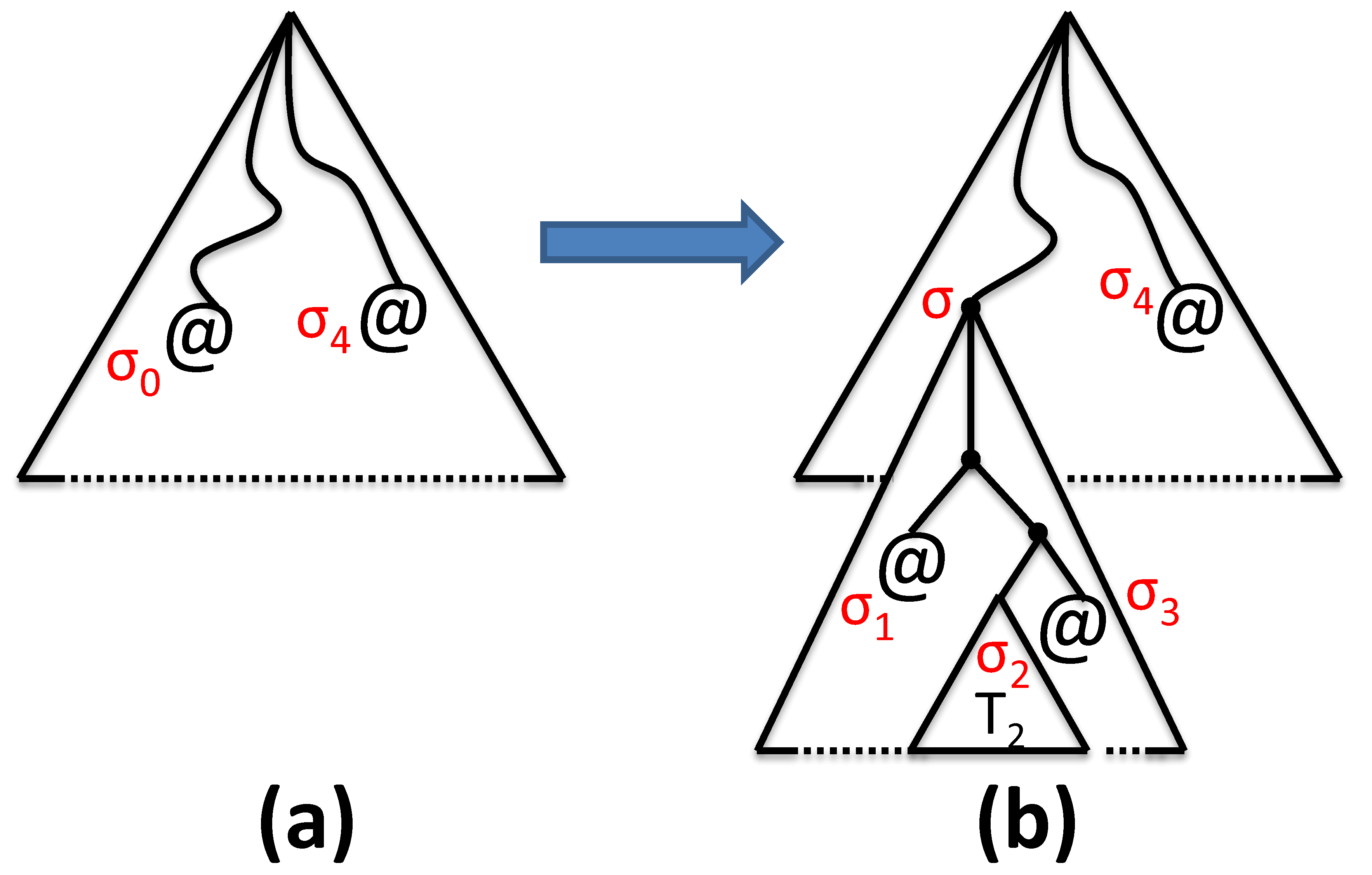
Figure 1: The Refinement Step

2.1 An Abstract Example

We now walk through the HSET refinement process on an abstract example, in Figure 1(a). The leftmost AI node @ with upper bound $\sigma_{0}$ is refined into the subtree labelled with the upper-bound analysis $\sigma$ in the second tree in Figure 1(b). Note that this new subtree contains two AI nodes with upper bounds $\sigma_{1}$ and $\sigma_{3}$. Note also that the subtree T2 does not contain any AI-nodes, and so $\sigma_{2}$ is also an exact analysis. We now detail this refinement.

Next consider the AI node labelled $\sigma_{0}$ in the first tree. Though this is a single node, we assume that the AI algorithm that gave rise to its analysis $\sigma_{0}$ also gave information about its extremal path, say $p$. Suppose this path, when expanded out from that single node, would go through the subtree $T_{2}$ indicated in the second tree. We then construct the subtree starting from $\sigma_{0}$ by first constructing the edges and nodes as a symbolic path p. As each edge and destination node is constructed from a branching source node, we also construct a new edge and destination node corresponding to the alternative of the branch. For this second destination node, which is not in the path p, we now construct a new AI node. At the end of this process, we would have constructed the subtree which has a spine corresponding to the path p, and along the spine, we have constructed a number of AI nodes (two, in this example, labelled $\sigma_{1}$ and $\sigma_{3}$).

See Figure Figure 1(b) and once again focus on the subtree labelled $\sigma$, and where the spine is some path that includes $\sigma_{2}$. There are two possible benefits of this refinement step. One is that this sub-HSET $\sigma$ is more precise than the original analysis $\sigma_{0}$ because the join of $\sigma_{1},\sigma_{2}$ and $\sigma_{3}$ is more precise than $\sigma_{0}$. Another benefit is when $\sigma_{2}$, which is an exact analysis, can be used to dominate any other analysis. For example, if the upper bound of $\sigma_{4}$ is less than the analysis of $\sigma_{2}$, then the entire subtree at $\sigma_{4}$ can be pruned from further consideration.

We remark here in the refinement step, each of the newly generated AI nodes require an (abstract) analysis, and although these analyses are efficient, there is the issue that the number of analyses could be as long as the path p. However, an important feature is that in the several invocations of abstract analysis performed here over the several AI nodes, and because the employed abstract domain is coarse, the analysis of each of these is often produces the the same results, and hence can be cached and need not be redone. We will argue and demonstrate this important feature in detail later.

2.2 A Motivating Example: Feasibility

Consider the program and its SET in Figure 2 and the WCET problem at hand is to determine the upper bound of tick. Assuming that any boolean combination of the unspecified guards $b_{i}$ is satisfiable. Then clearly the WCET is $6$, obtained from the leftmost path.

$\langle$0$\rangle$ $\mbox{\frenchspacing\it tick}=0$

$\langle$1$\rangle$ if ($b_{1}$) $\mbox{\frenchspacing\it tick}+\!\!=3$

$\langle$2$\rangle$ if ($b_{2}$) $\mbox{\frenchspacing\it tick}+\!\!=2$

$\langle$3$\rangle$ if ($b_{3}$) $\mbox{\frenchspacing\it tick}+\!\!=1$

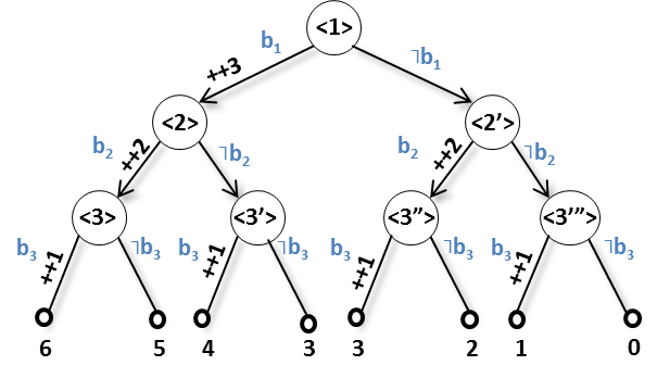
Figure 2: Example Program and its Symbolic Execution tree

To demonstrate reuse, assume that $\neg b_{1}\wedge b_{2}\wedge b_{3}$ is satisfiable, and that we already have an exact analysis, $\mbox{\frenchspacing\it tick}=3$ of the right subtree marked $\langle$2’$\rangle$. We now can produce an exact analysis for the left subtree marked $\langle$2$\rangle$ without having to traverse it. To do this, we take the longest path in the right subtree which gave rise to the analysis, i.e., the witness path, and this is the leftmost path under $\langle$2’$\rangle$. Call this path $p_{1}$. We now replay this path in the left subtree, getting the leftmost path starting from the root. Call this path $p_{2}$. Now the idea is that the analysis of $p_{2}$ is computed from the analysis of $p_{1}$, which is $3$. However, since the prefix of $p_{1}$ from the root to node $\langle$2’$\rangle$, which increments tick by zero, differs from the prefix of $p_{2}$ from the root to node $\langle$2$\rangle$, which increments tick by $3$, we must adjust for this and now declare that the exact analysis of node $\langle$2$\rangle$ is $\mbox{\frenchspacing\it tick}=6$. In other words, we assumed that the longest increment of tick from node $\langle$2$\rangle$ downwards is the same as that from node $\langle$2’$\rangle$, which is $3$. But since the prefix of node $\langle$2$\rangle$ is 3 more than the prefix of node $\langle$2’$\rangle$, we add a further $3$ to obtain the final value $6$.

There are two further points to note about reuse.

• If $b_{1}\wedge b_{2}\wedge b_{3}$ (ie. the leftmost path) were unsatisfiable, reuse is in fact still sound, when we declare that the analysis of node $\langle$2$\rangle$ is $6$. But may be imprecise. To prevent imprecision, we check that the path under node $\langle$2$\rangle$ that corresponds to the “witness” is feasible.

• Now suppose $\neg b_{1}\wedge b_{2}\wedge b_{3}$ (leftmost path in the right subtree) is unsatisfiable but $b_{1}\wedge b_{2}\wedge b_{3}$ (leftmost path in the left subtree) is satisfiable. Now it is unsound to reuse the exact analysis of node $\langle$2’$\rangle$ (which now is different from $3$) in the analysis of node $\langle$2$\rangle$. In previous implementations of reuse, e.g.: Jaffar et al. [2008, 2012]; Chu and Jaffar [2011], the exact analysis would be accompanied by an interpolant which would ensure that the reuse can soundly take place.

Our algorithm provides bounds for tick in each node. For example, an upper-bound analysis for the left subtree in Figure 2, labelled $\langle$2$\rangle$, is $\mbox{\frenchspacing\it tick}\leq 6$. This subtree also can have a lower-bound analysis of a nonnegative number less than or equal to $6$; We also can have a lower bound. for example, if the path proceeding to the left successor of $\langle$3’$\rangle$ was feasible, $4\leq\mbox{\frenchspacing\it tick}$ would be a lower bound. If however we did not care to check the feasibility of any path going through $\langle$2$\rangle$, then we could quickly estimate that $3$ is a lower bound (by choosing only rightmost branches that do not add to tick). Note that there may not actually be a real execution path resulting in $\mbox{\frenchspacing\it tick}=3$. Note also that lower bounds whose values are too low (e.g., $0\leq\mbox{\frenchspacing\it tick}$) are not very useful.

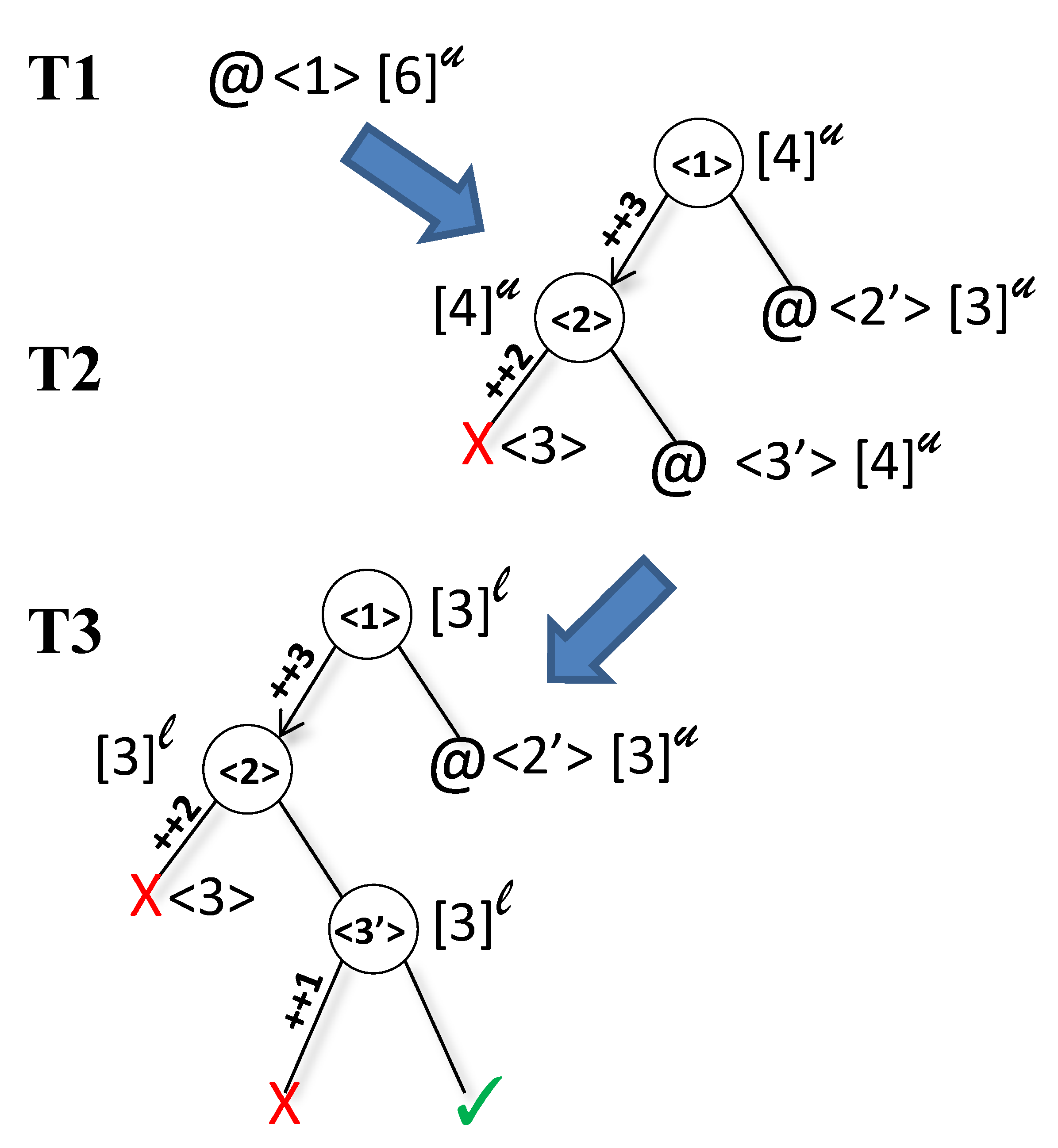
Figure 3: Detailed Refinement Step

We now proceed to analyze the program incrementally. See Figure 3 where “@” denotes an AI node, the $l$ and $u$ superscripts denote lower and upper bounds respectively, and the $T_{i}$s represent the HSET we construct in each iteration. We start with a single AI node at $T_{1}$ representing an (abstract) analysis of the program starting at the beginning. We could have used traditional abstract interpretation (AI) which over-approximates the set of paths in the SET in order to limit consideration to a small number of abstract states (typically, one state per program point). Thus AI analyzers are typically very efficient. We then quickly, because the analyzer is path-insensitive, determine a (trivial) lower bound of $0$ and an upper bound of $6$. Furthermore, the analyzer indicates that the leftmost path is a witness path, i.e., if it were feasible, then it would indicate the true WCET. In Figure 3, we show only upper bounds when the lower bound is trivial.

Next we refine the single AI node $T_{1}$ into the HSET $T_{2}$ which now contains new nodes, amongst them two AI nodes at $\langle$2’$\rangle$ and $\langle$3’$\rangle$. Using abstract interpretation, note that former has an upper bound of $3$, while the latter has an upper bound of $4$. We assume that the constraint $b_{1}\wedge b_{2}$ is unsatisfiable, and so the leftmost path in Figure 2 is in fact infeasible (at just before program point $\langle$3$\rangle$). Now since node $\langle$3’$\rangle$ has a bound $4$, this is inherited by the parent node $\langle$2$\rangle$. Finally, the root node $\langle$1$\rangle$ inherits the larger of the bounds of its successors, which are $3$ and $4$, and so we obtain a final bound of $4$. Now since $T_{2}$ contains AI nodes which contribute to this answer, this analysis is not confirmed to be exact.

Finally we deal with the two remaining AI nodes in $T_{2}$, and choose one of them to refine. We choose the node $\langle$3’$\rangle$ over $\langle$2’$\rangle$ because its upper bound is higher. The intuition is this: if we instead chose to refine the AI node with the smaller bound, the other AI node will still need to refined in the future. If, as we will show next, we choose the AI node $\langle$3’$\rangle$ with the higher bound, there is a chance that the remaining AI node can be dominated. We now obtain $T_{3}$ by refining this AI node.

This refinement produced two successors, and by assuming that the constraint $b_{1}\wedge\neg b_{2}\wedge b_{3}$ is unsatisfiable, we have that the left subtree of node $\langle$3’$\rangle$ is an infeasible path. The right subtree is a terminal node, and so for the first time, we can declare that, since both subtrees of $\langle$3’$\rangle$ have no AI-nodes, $\langle$3’$\rangle$ has a lower bound of $3$. The most interesting step now can be taken: the analysis here dominates the analysis at the one remaining AI node at $\langle$2’$\rangle$. Note that the set of paths represented by $\langle$2’$\rangle$ is nearly half of all the paths. By pruning away this subtree, we now have that the entire tree has no more AI nodes, and we can now declare that the root node has an exact analysis of $3$.

2.3 A Motivating Example: Optimality

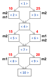
(a) CFG

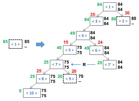
(b) Detailed Refinement Step

Figure 4: Example: WCET Analysis with Cache. The list of pair in (b) is just to simplify the presentation.

We now consider an example with a dynamic cost model. In particular, consider WCET analysis of the program, whose Control Flow Graph (CFG) is shown in Fig. 4(a). Each node – rectangular box – represents a basic block. In the basic blocks, $\mbox{{\color[rgb]{0,0,1}{$\langle$1$\rangle$}}},\mbox{{\color[rgb]{0,0,1}{$\langle$2$\rangle$}}},\dots\mbox{{\color[rgb]{0,0,1}{$\langle$10$\rangle$}}}$ denote the program points. While the timings of basic blocks $\mbox{{\color[rgb]{0,0,1}{$\langle$1$\rangle$}}},\mbox{{\color[rgb]{0,0,1}{$\langle$4$\rangle$}}},\mbox{{\color[rgb]{0,0,1}{$\langle$7$\rangle$}}},\mbox{{\color[rgb]{0,0,1}{$\langle$10$\rangle$}}}$ are always $0$, other basic blocks are abstracted by the static timing of the instructions in cycles, denoted by a non-negative integer (placed above each node, in red), and a sequence of memory accesses $m_{i}$, of which the timing depends on the cache configuration at the time of access. (In the beginning the cache is empty.)

For simplicity, we assume: (1) direct-mapped cache; (2) $m_{1}$ and $m_{2}$ map to the same cache location, i.e., they conflict; (3) a cache miss costs $10$ cycles, while a cache hit costs $0$. Given the setting, it is clear that the timing of a single symbolic path can be precisely determined. Thus if we exhaustively enumerate the symbolic execution tree, exact analysis can be achieved. However, such approach is prohibitive in practice.

We now assume that the base Abstract Interpretation (AI) used is the must-analysis abstract cache proposed by Theiling et al. [2000]. To distinguish our approach from a large body of work in program verification, we assume that all the symbolic paths in the program are feasible. In other words, simply refining on the (in)feasibility of paths will not improve the analysis precision.

Phase 1: we start by invoking AI at $\langle$1$\rangle$. Note that cache merging is perform at every join point. While we can determine precisely that the accesses in $\langle$2$\rangle$, likewise the access in $\langle$3$\rangle$, are all misses, the merge at $\langle$4$\rangle$ keeps neither $m_{1}$ nor $m_{2}$ in the must-cache. Similarly, we can determine the accesses in $\langle$5$\rangle$ and $\langle$6$\rangle$ as all misses. However, going through either $\langle$5$\rangle$ or $\langle$6$\rangle$, both paths end up with $m_{2}$ in the cache, thus the merge at $\langle$7$\rangle$ keeps $m_{2}$. Following up, the access to $m_{1}$ at $\langle$8$\rangle$ is a miss, while the access to $m_{2}$ at $\langle$9$\rangle$ is a hit.

In summary, the AI algorithm can give us an analysis for each program point, summarizing the estimate of the WCET from that point to the end of the program:

($\langle$10$\rangle$, 0), ($\langle$9$\rangle$, 20), ($\langle$8$\rangle$, 25), ($\langle$7$\rangle$, 25), ($\langle$6$\rangle$, 49),
($\langle$5$\rangle$, 50), ($\langle$4$\rangle$, 50), ($\langle$3$\rangle$, 85), ($\langle$2$\rangle$,80), ($\langle$1$\rangle$, 85),

where (B,T) means that T is the estimated worst-case timing from B to the end of the program. In other words, invoking AI at $\langle$1$\rangle$, we achieve the analysis of 85 (= 35 + 25 + 25), and the extremal trace witnessing that analysis is:

$\mbox{{\color[rgb]{0,0,1}{$\langle$1$\rangle$}}}\rightarrow\mbox{{\color[rgb]{0,0,1}{$\langle$3$\rangle$}}}\rightarrow\mbox{{\color[rgb]{0,0,1}{$\langle$4$\rangle$}}}\rightarrow\mbox{{\color[rgb]{0,0,1}{$\langle$5$\rangle$}}}\rightarrow\mbox{{\color[rgb]{0,0,1}{$\langle$7$\rangle$}}}\rightarrow\mbox{{\color[rgb]{0,0,1}{$\langle$8$\rangle$}}}\rightarrow\mbox{{\color[rgb]{0,0,1}{$\langle$10$\rangle$}}}$.

Phase 2: At the end of phase 1, our HSET contains only one abstract node as in Fig. 4(b). We denote abstract nodes using dashed boxes. Every node in our HSET, when applicable, will be annotated with 3 pieces of information:

1. the current estimate of the WCET from the node to the end of the program – on the left, in green color;

2. the aggregated lower bound analysis of all the paths through this node – on the right and below; and

3. the aggregated upper bound analysis of all the paths passing through this node – on the right and above;

We proceed refining by first building a “spine” targeting the extremal trace identified in the previous phase. This (first) spine is shown as the left most path in Fig. 4(b). Note that at the end of the path, the analysis of $\langle$10$\rangle$ is exact, but the access $m_{2}$ at $\langle$5$\rangle$ has now resolved to be a hit (instead of a miss), the annotation at $\langle$10$\rangle$ is therefore $0,[75]^{l},[75]^{u}$ as shown. Similarly, the annotation at $\langle$8$\rangle$ is $25,[75]^{l},[75]^{u}$. Note that the execution time of each block has been updated in Fig. 4(b) considering the context in which it is executed.

Now, we need to deal with analysis of the sibling node, at program point $\langle$9$\rangle$. However, it is easy to see that if we use the coarse estimate returned from the previous phase for $\langle$9$\rangle$, domination happens, because the upper bound analysis of all paths going through that node is just 70 ($=35+15+{\bf 20}$). Correspondingly, the annotation for this node is $20,-,[70]^{u}$.

Propagating back, we see that along the spine, the analysis at $\langle$7$\rangle$ and $\langle$5$\rangle$ are now exact. We now consider the sibling of $\langle$5$\rangle$, which is $\langle$6$\rangle$. Using the coarse estimate for $\langle$6$\rangle$ from the previous phase, domination does not happen (because $35+{\bf 49}>75$). We do not invoke a new AI analysis from here, but proceed until the next join point. There are two reasons:

• reuse of an exact analysis might be possible, as we will see soon. In this case, we achieve precise analysis for the node, while also avoid a call to the base AI analysis.

• we can propagate information precisely till the join point (this is cheap), so that the call to AI might return better analysis than what has been achieved in the previous phases.

So we proceed to the node $\mbox{{\color[rgb]{0,0,1}{$\langle$7$\rangle$}}}^{\prime}$ in the figure. Note that at $\mbox{{\color[rgb]{0,0,1}{$\langle$7$\rangle$}}}^{\prime}$ we share the same cache context encountered before in $\langle$7$\rangle$, i.e., $m_{2}$ is present in the cache. Also note that since there are no infeasible paths, the interpolant Chu and Jaffar [2011] stored at $\langle$7$\rangle$ is simply $true$. Thus we can trivially reuse the exact analysis of $\langle$7$\rangle$ at $\mbox{{\color[rgb]{0,0,1}{$\langle$7$\rangle$}}}^{\prime}$. The annotation at $\mbox{{\color[rgb]{0,0,1}{$\langle$7$\rangle$}}}^{\prime}$ is then $25,[84]^{l},[84]^{u}$. The annotations for $\langle$6$\rangle$, $\langle$4$\rangle$, $\langle$3$\rangle$ can be computed from this by propagating it back.

Fast forwarding, for $\langle$2$\rangle$, using the previous estimate, domination happens, we then end up with the “exact” analysis for the whole program, as the annotation of $\langle$1$\rangle$ is $84,[84]^{l},[84]^{u}$.

2.4 Discussion on Scalability

We have already mentioned our algorithm is “anytime”, and further that it is progressive and consequently, the algorithm converges in the sense that it eventually produces an exact analysis. The main reason for this that an execution path is never be considered twice and so the search space is monotonically strictly decreasing. But of course this is not enough to attain scalability.

As mentioned above, for scalability, it is critical an algorithm which performs iterations that are progressively more expensive to be incremental. That is, the work done in previous iterations must be both (a) persistent and compact, (b) directly useful to mitigate the cost of the next iteration. We now overview how our algorithm addresses these criteria by some form of pruning of the search space.

Reuse of Abstract Analyses:
In the refinement of a node $v$ to produce a spine path of length $n$, we generally produce $n-1$ new AI nodes attached to the spine. However, it is typical in AI implementations (which was used on the node $v$) to have computed analysis for all program points that are reachable from $v$’s program point (via the CFG), and not just for that of the root $v$. Therefore much of the analyses required for the new AI nodes are typically already at hand.

Reuse of Exact Analyses:
Here we use a computed exact analysis of one subtree to derive an exact analysis of another subtree. Suppose we have an exact analysis $E$ for a subtree rooted at $v$. In this scenario, we exploit $E$ to compute another exact analysis $E^{\prime}$ for another (yet unexplored) node associated with the same program point as $v$. In general, the witness condition for such a reuse (here we are talking about real witnesses for the exact analysis), as well as the precise definition of the mapping from $E$ to $E^{\prime}$, is quite involved because it depends on the kind of analysis in question. But in specific instances, this is easily done. We thus omit a full description here but instead refer to Jaffar et al. [2008]; Chu and Jaffar [2011]; Jaffar et al. [2012], and use an example of reuse in Section 2.

Domination:
Suppose we have a nontrivial lower-bound analysis, say for node $v$. Now we can in fact prune all subtrees which are dominated by $v$. Note that domination does not require that the two entities involved represent the same program point, in contrast to reusing. In other words, any node/subtree can dominate any other. Another difference between reuse and domination is that both parties involved in a reuse contribute an analysis; it is just that we have a quick way to compute one of them from the other. Domination however means that we can simply ignore the dominated party.

In the end, during the refinement process, the effects of reuse and domination serve to prune the search space, while the increasing level of exact analyses of subspaces. This produces more lower-bound analyses, and these, in turn, produce better upper bounds, and this in turn, creates further opportunities for reuse and domination. This cycle of mutual benefits is the key to the scalability of our algorithm.

3 Hybrid Symbolic Execution with Interpolation

Here we provide the formalities required for our algorithm. In particular, we cover the needed aspects of symbolic execution, abstract interpretation and interpolation. We also highlight some important assumptions.

Syntax. We restrict our presentation to a simple imperative programming language where all basic operations are either assignments or assume operations, and the domain of all variables is the integers. The set of all program variables is denoted by Vars. An assignment x := e corresponds to assigning the evaluation of the expression e to the variable x. In the assume operator, assume(c), if the boolean expression c evaluates to true, then the program continues, otherwise it halts. The set of operations is denoted by Ops. We then model a program by a transition system. A transition system is a quadruple $\langle{\mbox{$\Sigma$}},{\mbox{$\mbox{$\ell$}_{\textsf{start}}$}},{\longrightarrow},{O}\rangle$ where $\Sigma$ is the set of program points and $\mbox{$\mbox{$\ell$}_{\textsf{start}}$}\in\mbox{$\Sigma$}$ is the unique initial program point. $\longrightarrow\subseteq\mbox{$\Sigma$}\times\mbox{$\Sigma$}\times\mbox{\emph{Ops}}$ is the transition relation that relates a state to its (possible) successors executing operations. This transition relation models the operations that are executed when control flows from one program point to another. We shall use $\mbox{$\ell$}~{}\xlongrightarrow[]{\textsf{op}}~{}\mbox{$\ell$}^{\prime}$ to denote a transition relation from $\mbox{$\ell$}\in\mbox{$\Sigma$}$ to $\mbox{$\ell$}^{\prime}\in\mbox{$\Sigma$}$ executing the operation $\textsf{op}\in\mbox{\emph{Ops}}$. Finally, $O\subseteq\mbox{$\Sigma$}$ is the set of terminal program points.

Symbolic Execution (SE). A symbolic state $v$ is usually defined as a triple $\langle{\mbox{$\ell$}},{\mbox{$s$}},{\mbox{$\Pi$}}\rangle$. The symbol $\mbox{$\ell$}\in\mbox{$\Sigma$}$ corresponds to the current program point. The symbolic store $s$ is a function from program variables to terms over input symbolic variables. The evaluation $\llbracket{c}\rrbracket_{\mbox{$s$}}$ of a constraint expression $c$ in a store $s$ is defined as: $\llbracket{x}\rrbracket_{\mbox{$s$}}=s(x)$ (if $x$ is a variable), $\llbracket{n}\rrbracket_{\mbox{$s$}}=n$ (if $n$ is an integer), $\llbracket{e~{}{\sf op}~{}e^{\prime}}\rrbracket_{\mbox{$s$}}=\llbracket{e}\rrbracket_{\mbox{$s$}}~{}{\sf op}~{}{\llbracket{e^{\prime}}\rrbracket_{\mbox{$s$}}}$ (where $e,e^{\prime}$ are expressions and op is a relational or arithmetic operator). $\Pi$ is called path condition and it is a first-order formula over the symbolic inputs and it accumulates constraints which the inputs must satisfy in order for an execution to follow the particular corresponding path. The set of first-order formulas and symbolic states are denoted by FO and SymStates, respectively.

For all purposes of this paper, we do not consider arbitrary symbolic states, but only those generated during our symbolic execution. For technical reasons, we require a symbolic state to be aware of how it is reached in the symbolic execution tree. Hence, we abuse notation to (re)define a symbolic state as follows.

Definition 1 (Symbolic State)

A symbolic state $v$ is a quadruple $\langle{\mbox{\mbox{$\ell$}}},{\mbox{$s$}},{\mbox{$\Pi$}},{\mbox{$\pi$}}\rangle$, where $\ell$, $s$, $\Pi$ are as before while the additional parameter $\pi$ is a sequence of program transitions that were taken during Symbolic Execution in order to reach $v$. $\Box$

Definition 2 (Transition Step)

Given a transition system $\langle{\mbox{$\Sigma$}},{\mbox{$\mbox{$\ell$}_{\textsf{start}}$}},{\longrightarrow},{O}\rangle$ and a state $\mbox{$v$}\equiv\langle{\mbox{\mbox{$\ell$}}},{\mbox{$s$}},{\mbox{$\Pi$}},{\mbox{$\pi$}}\rangle\in\mbox{\emph{SymStates}}$, the symbolic execution of $\mbox{$\ell$}~{}\xlongrightarrow[]{\textsf{op}}~{}\mbox{$\ell$}^{\prime}$ returns another symbolic state $\mbox{$v$}^{\prime}$ defined as:

${\sf SYMSTEP}(\mbox{$v$},\mbox{\mbox{$\ell$}}~{}\xlongrightarrow[]{\sf op}~{}\mbox{\mbox{$\ell$}}^{\prime})\equiv\mbox{$v$}^{\prime}\mbox{~{}$\triangleq$~{}}$

$$\left\{\begin{array}[]{ll}\langle{\mbox{\mbox{$\ell$}}^{\prime}},{\mbox{$s$}},{\mbox{$\Pi$}\wedge\llbracket{c}\rrbracket_{\mbox{$s$}}},{\mbox{$\pi$}^{\prime}}\rangle&\textup{if {op} $\equiv$ \mbox{{assume(c)}} and $\mbox{$\Pi$}\wedge\llbracket{c}\rrbracket_{\mbox{$s$}}$}\\ &\textup{is satisfiable}\\ \langle{\mbox{\mbox{$\ell$}}^{\prime}},{\mbox{$s$}[x\mapsto\llbracket{e}\rrbracket_{\mbox{$s$}}]},{\mbox{$\Pi$}},{\mbox{$\pi$}^{\prime}}\rangle&\textup{if {op} $\equiv$ \mbox{{x := e}}}\\ \end{array}\right.$$ (4)

where $\mbox{$\pi$}^{\prime}\mbox{~{}$\triangleq$~{}}\ \mbox{$\pi$}~{}\cdot~{}\mbox{\mbox{$\ell$}}~{}\xlongrightarrow[]{\sf op}~{}\mbox{\mbox{$\ell$}}^{\prime}$. We call $\mbox{$v$}^{\prime}$ a successor of $v$. $\Box$

Note that Eq. (4) queries a theorem prover for satisfiability checking on the path condition. In practice, we assume the theorem prover is sound but not necessarily complete. That is, the theorem prover must say a formula is unsatisfiable only if it is indeed so. Given a symbolic state $\mbox{$v$}\equiv\langle{\mbox{\mbox{$\ell$}}},{\mbox{$s$}},{\mbox{$\Pi$}},{\mbox{$\pi$}}\rangle$ we define $\mbox{$\llbracket{\mbox{$v$}}\rrbracket$}:\mbox{\emph{SymStates}}~{}\mbox{$\rightarrow$}~{}\mbox{\emph{FO}}$ as the formula $(\bigwedge_{v~{}\in~{}\mbox{\emph{Vars}}}~{}\llbracket{v}\rrbracket_{\mbox{$s$}})\wedge\mbox{$\Pi$}$ where Vars is the set of program variables. Such projection step is performed by eliminating existentially all auxiliary variables that are not in Vars. As a convention, we use $\circ$ in a tuple to denote a value that we are not interested in.

A symbolic path $\mbox{$v$}_{0}\cdot\mbox{$v$}_{1}\cdot...\cdot\mbox{$v$}_{n}$ is a sequence of symbolic states such that $\forall i\bullet 1\leq i\leq n$ the state $\mbox{$v$}_{i}$ is a successor of $\mbox{$v$}_{i-1}$. A path $\mbox{$v$}_{0}\cdot\mbox{$v$}_{1}\cdot...\cdot\mbox{$v$}_{n}$ is feasible if $\mbox{$v$}_{n}\equiv\langle{\mbox{\mbox{$\ell$}}},{\mbox{$s$}},{\mbox{$\Pi$}},{\mbox{{$\circ$}}}\rangle$ such that $\llbracket{\mbox{$\Pi$}}\rrbracket_{\mbox{$s$}}$ is satisfiable. If $\mbox{\mbox{$\ell$}}\in O$ and $\mbox{$v$}_{n}$ is feasible then $\mbox{$v$}_{n}$ is called terminal state, denoted TERMINAL($\mbox{$v$}_{n}$). Otherwise, if $\llbracket{\mbox{$\Pi$}}\rrbracket_{\mbox{$s$}}$ is unsatisfiable the path is called infeasible and $\mbox{$v$}_{n}$ is called an infeasible state, denoted INFEASIBLE($\mbox{$v$}_{n}$). If there exists a feasible path $\mbox{$v$}_{0}\cdot\mbox{$v$}_{1}\cdot...\cdot\mbox{$v$}_{n}$ then we say $\mbox{$v$}_{k}$ ($0\leq k\leq n$) is reachable from $\mbox{$v$}_{0}$ in k steps. We say $\mbox{$v$}^{\prime}$ is reachable from $v$ if it is reachable from $v$ in some number of steps. A symbolic execution tree contains all the execution paths explored during the symbolic execution of a transition system by triggering Eq. (4). The nodes represent symbolic states and the arcs represent transitions between states.

Assumption 1

Given a terminal state $\mbox{$v$}\equiv\langle{\mbox{\mbox{$\ell$}}},{\mbox{$s$}},{\mbox{$\Pi$}},{\mbox{$\pi$}}\rangle$, we assume the existence of a function $\theta$ which extracts from $\pi$ an “exact” analysis $\theta(\mbox{$\pi$})$. $\Box$

This exactness is a theoretical concept that helps us quantify the precision of our incremental analysis against a fully path- and context-sensitive algorithm. We note that such algorithms do exist for loop-free programs, but they often do not work in the setting of realistic memory/timing budget.

Abstract Interpretation (AI). An invocation of AI at a symbolic state $v$ constructs an AI node at $v$, using an abstract domain $\mathcal{A}$, which is assumed to be a lattice. This step starts by making use of the abstraction function $\alpha$ to map the current symbolic state $v$ to an abstract value, i.e., computing $\alpha$($v$), then performing a standard AI computation over $\mathcal{A}$ and the input CFG.

Assumption 2

We expect an invocation of AI would necessarily return an upper bound analysis $\mathcal{U}$, i.e., a safe over-approximation, of the set of paths through $v$. In addition, we also assume that it produces witness paths denoted as $\omega$ – a set of paths from which the upper bound analysis $~{}\mathcal{U}$ is derived. $\Box$

For WCET analysis, $\omega$ contains only one path. But for general analyses, $\omega$ often is just a small subset of all the paths going through $v$, since not all paths contribute to the returned analysis $\mathcal{U}$.

Assumption 3

We assume the analysis values also form a lattice structure ${\cal R}$, or $[{{\cal S},\sqsubseteq},{\bot},{\sqcup},{\sqcap},{\top}]$, where ${\cal S}$ is the set of analysis values, $\sqsubseteq$ is the partial order relationship, $\sqcup$ and $\sqcap$ are the least upper bound and greatest lower bound operators, and $\bot$ and $\top$ are the bottom and top elements of the lattice respectively. We assume that $\sqcup$ is precise so that exact analyses over different paths can be combined precisely, yielding an exact analysis over the collection of paths. $\Box$

Note that unlike the abstract domain $\mathcal{A}$ to run AI, ${\cal R}$ does not concern (partially) the (in-)feasibility of the program paths. While $\mathcal{A}$ is typically designed to be coarse enough so that an invocation of AI is fast, ${\cal R}$ is designed with precision in mind. In practice, this does not hamper the overall scalability of our algorithm, since operations on the analysis values defined by ${\cal R}$ are performed only a small number of times, bounded by the number of nodes in the HSET. (In other words, this assumption does not add any extra complexity to our algorithm.)

To simplify the presentation of the hybrid symbolic execution tree (HSET), we also assume that an invocation of AI also returns a lower bound analysis $\mathcal{L}$. In practice, one can always make use of a trivial lower bound, e.g., $\bot$. Let $\mathcal{E}$ be the desired exact analysis of the set of paths, then $\mathcal{L}\sqsubseteq\mathcal{E}\sqsubseteq\mathcal{U}$ (we do not explicitly compute $\mathcal{E}$ but infer it when $\mathcal{L}$ and $\mathcal{U}$ coincide).

It now should be clear that under our notion of exactness and the above assumptions, the analysis for each terminal symbolic state $\mbox{$v$}\equiv\langle{\mbox{\mbox{$\ell$}}},{\mbox{$s$}},{\mbox{$\Pi$}},{\mbox{$\pi$}}\rangle$ is exact. Its lower bound and upper bound coincide at $\theta(\mbox{$\pi$})$.

We comment here that computing the witness paths is straightforward but tedious, so we do not detail it here. Typically an AI algorithm operates over a CFG. During its execution, it can “mark” certain edges in the CFG that are sufficient to produce the analysis of the target AI node where the analysis is invoked. The witness paths can then be obtained by traversing marked edges from the target AI node to a terminal node (of the CFG). One can also follow Cerny et al. [2013] to get not only the upper bound analysis, but also the extremal path(s) from an abstract computation (within an iteration). In summary, it is reasonable to assume the existence of a procedure AbstractInterpretation which when invoked with a symbolic state $v$ returns a triple $\langle{\mathcal{L}},{\mathcal{U}},{\mbox{$\omega$}}\rangle$.

Interpolation. Given a pair of first order logic formulas $A$ and $B$ such that $A\wedge B$ is $false$, an interpolant Craig [1955] is another formula $\overline{\Psi}$ such that (a) $A\models\mbox{$\overline{\Psi}$}$, (b) $\mbox{$\overline{\Psi}$}\wedge B$ is false, and (c) $\overline{\Psi}$ is formed using common variables of $A$ and $B$. An interpolant removes irrelevant information in $A$ that is not needed to maintain the unsatisfiability of $A\wedge B$.

Interpolation has been prominently used to reduce state space blowup in both program verification McMillan [2010]; Jaffar et al. [2009] and program analysis Chu and Jaffar [2011]; Jaffar et al. [2012]. Here we will use it for a similar purpose – to merge, or subsume, symbolic states and avoid redundant exploration. During symbolic execution, our algorithm will annotate certain states with an interpolant, which can be used to prune other symbolic trees.follows.

Definition 3 (Subsumption)

Given a current symbolic state $\mbox{$v$}\equiv\langle{\mbox{\mbox{$\ell$}}},{\mbox{$s$}},{\mbox{{$\circ$}}},{\mbox{{$\circ$}}}\rangle$ and an already explored symbolic state at the same program point $\mbox{$v$}^{\prime}\equiv\langle{\mbox{\mbox{$\ell$}}},{\mbox{{$\circ$}}},{\mbox{{$\circ$}}},{\mbox{{$\circ$}}}\rangle$ annotated with the interpolant $\overline{\Psi}$, we say $\mbox{$v$}^{\prime}$ subsumes $v$, denoted as ${\sf SUBSUMES}(\mbox{$v$}^{\prime},\mbox{$v$})$ if (a) $\llbracket{\mbox{$v$}}\rrbracket_{\mbox{$s$}}\models\mbox{$\overline{\Psi}$}$ and (b) $\mbox{$\alpha$}(\mbox{$v$})\sqsubseteq\mbox{$\alpha$}(\mbox{$v$}^{\prime})$.

The first condition ensures that the symbolic paths through $v$ are a subset of the symbolic paths through $\mbox{$v$}^{\prime}$, and the second condition ensures that the HSET at $\mbox{$v$}^{\prime}$ has already been explored with a more general context $\mbox{$\alpha$}(\mbox{$v$}^{\prime})$. Therefore, by exploring $v$ one cannot obtain a more precise analysis than that has been already obtained by exploring $\mbox{$v$}^{\prime}$, and hence $v$ can be subsumed.

We note that subsumption is a special form of reuse that has been briefly discussed in the early Sections. While reuse (with interpolation) has been exploited for different analysis problems Chu and Jaffar [2011]; Jaffar et al. [2012], formulating this concept for a general analysis framework is rather involved. For simplicity, we thus omit the detail.

To conclude this Section, we comment that efficient interpolation algorithms do exist for quantifier-free fragments of theories such as linear real/integer arithmetic, uninterpreted functions, pointers and arrays, and bitvectors (e.g., see Cimatti et al. [2008] for details) where interpolants can be extracted from the refutation proof in linear time on the size of the proof.

4 Algorithm

IncrementalAnalysis ($P$) 1: $\mbox{$v$}\ \mbox{:=}\ \langle{\mbox{$\mbox{$\ell$}_{\textsf{start}}$}},{\emptyset},{\mbox{\frenchspacing\it true}},{\mbox{{$\circ$}}}\rangle$ 2: $\langle{\mathcal{L}},{\mathcal{U}},{\mbox{$\omega$}}\rangle$ := AbstractInterpretation ($v$) 3: do 4: $R\ \mbox{:=}\ \{\mbox{$v$}~{}|~{}\nexists\ \mbox{$v$}^{\prime}$ s.t. ${\sf DOMINATES}(\mbox{$v$}^{\prime},\mbox{$v$})\}$ 5: $\mbox{$v$}\ \mbox{:=}\ \emph{RefinementHeuristic}\ (R)$ 6: let $\langle{\mathcal{L}},{\mathcal{U}},{\mbox{$\omega$}},{\mbox{$\overline{\Psi}$}}\rangle$ be the annotation at $v$ 7: select a witness path $\sigma_{\mbox{$v$}}$ from $\omega$ 8: spine_done := false; RefineUnfold($v$, $\sigma_{\mbox{$v$}}$) 9: PropagateBack($v$) 10: until BoundsHeuristic PropagateBack ($\mbox{$v$}^{\prime}\equiv\langle{\mbox{\mbox{$\ell$}}},{\mbox{{$\circ$}}},{\mbox{{$\circ$}}},{\mbox{{$\circ$}}}\rangle$) 11: if $\mbox{\mbox{$\ell$}}\ \equiv\ \mbox{$\mbox{$\ell$}_{\textsf{start}}$}$ then return 12: let $v$ be the predecessor of $\mbox{$v$}^{\prime}$ 13: $\langle{\mathcal{L}},{\mathcal{U}},{\mbox{$\omega$}},{\mbox{$\overline{\Psi}$}}\rangle\mbox{:=}\ \langle{\bot},{\bot},{\emptyset},{\mbox{\frenchspacing\it true}}\rangle$ 14: foreach successor $\mbox{$v$}^{\prime\prime}$ of $v$ wrt. the transition $\mbox{\mbox{$\ell$}}~{}\xlongrightarrow[]{\sf op}~{}\mbox{\mbox{$\ell$}}^{\prime\prime}$ 15: let $\langle{\mathcal{L}^{\prime\prime}},{\mathcal{U}^{\prime\prime}},{\mbox{$\omega$}^{\prime\prime}},{\mbox{$\overline{\Psi}$}^{\prime\prime}}\rangle$ be the annotation at $\mbox{$v$}^{\prime\prime}$ 16: $\langle{\mathcal{L}},{\mathcal{U}},{\mbox{$\omega$}}\rangle$ :=  Combine($\langle{\mathcal{L}},{\mathcal{U}},{\mbox{$\omega$}}\rangle$, $\langle{\mathcal{L}^{\prime\prime}},{\mathcal{U}^{\prime\prime}},{\mbox{$\omega$}^{\prime\prime}}\rangle$) 17: $\mbox{$\overline{\Psi}$}\ \mbox{:=}\ \mbox{$\overline{\Psi}$}\wedge\mbox{{$\widehat{wlp}$}}~{}(\mbox{$\overline{\Psi}$}^{\prime\prime},{\sf op})$ 18: endfor 19: replace $v$’s annotation with $\langle{\mathcal{L}},{\mathcal{U}},{\mbox{$\omega$}},{\mbox{$\overline{\Psi}$}}\rangle$ 20: PropagateBack($v$) Combine ($\langle{\mathcal{L}_{1}},{\mathcal{U}_{1}},{\mbox{$\omega_{1}$}}\rangle$, $\langle{\mathcal{L}_{2}},{\mathcal{U}_{2}},{\mbox{$\omega_{2}$}}\rangle$) 21: $\mathcal{L}$ := $\mathcal{L}_{1}$ $\sqcup$ $\mathcal{L}_{2}$ 22: if $\mathcal{U}_{1}~{}\sqsubseteq~{}\mathcal{U}_{2}$  then $\omega$ := $\omega_{2}$ 23: else if $\mathcal{U}_{2}~{}\sqsubseteq~{}\mathcal{U}_{1}$  then $\omega$ := $\omega_{1}$ 24: else $\omega$  := $\mbox{$\omega_{1}$}~{}\cup~{}\mbox{$\omega_{2}$}$ 25: $\mathcal{U}$  :=  $\mathcal{U}_{1}$  $\sqcup$  $\mathcal{U}_{2}$ 26: return $\langle{\mathcal{L}},{\mathcal{U}},{\mbox{$\omega$}}\rangle$

RefineUnfold ($\mbox{$v$}\equiv\langle{\mbox{\mbox{$\ell$}}},{\mbox{{$\circ$}}},{\mbox{{$\circ$}}},{\mbox{$\pi$}}\rangle$, $\sigma_{\mbox{$v$}}$) 27: if INFEASIBLE ($v$) then 28: $\langle{\mathcal{L}},{\mathcal{U}},{\mbox{$\omega$}},{\mbox{$\overline{\Psi}$}}\rangle\mbox{:=}\ \langle{\bot},{\bot},{\emptyset},{\mbox{\frenchspacing\it false}}\rangle$; spine_done := true; 29: else if TERMINAL ($v$) then 30: $\langle{\mathcal{L}},{\mathcal{U}},{\mbox{$\omega$}},{\mbox{$\overline{\Psi}$}}\rangle\mbox{:=}\ \langle{\theta(\mbox{$\pi$})},{\theta(\mbox{$\pi$})},{\emptyset},{\mbox{\frenchspacing\it true}}\rangle$; spine_done := true 31: $\mbox{{else}}\ \mbox{{if}}\ (\exists\ \mbox{$v$}^{\prime}\equiv\langle{\mbox{\mbox{$\ell$}}},{\mbox{{$\circ$}}},{\mbox{{$\circ$}}},{\mbox{{$\circ$}}}\rangle$ s.t. $\mbox{$v$}^{\prime}$ is annotated $\langle{\mathcal{L}^{\prime}},{\mathcal{U}^{\prime}},{\mbox{$\omega$}^{\prime}},{\mbox{$\overline{\Psi}$}^{\prime}}\rangle$                                         and ${\sf SUBSUMES}~{}(\mbox{$v$}^{\prime},\mbox{$v$}))$ then 32: $\langle{\mathcal{L}},{\mathcal{U}},{\mbox{$\omega$}},{\mbox{$\overline{\Psi}$}}\rangle$ := $\langle{\mathcal{L}^{\prime}},{\mathcal{U}^{\prime}},{\mbox{$\omega$}^{\prime}},{\mbox{$\overline{\Psi}$}^{\prime}}\rangle$; spine_done := true 33: else if spine_done then 34: $\langle{\mathcal{L}},{\mathcal{U}},{\mbox{$\omega$}}\rangle$ := $\textsc{AbstractInterpretation}(\mbox{$v$})$;  $\overline{\Psi}$  :=  true 35: else 36: $\langle{\mathcal{L}},{\mathcal{U}},{\mbox{$\omega$}},{\mbox{$\overline{\Psi}$}}\rangle\mbox{:=}\ \langle{\bot},{\bot},{\emptyset},{\mbox{\frenchspacing\it true}}\rangle$ 37: select a transition s.t. $\mbox{\mbox{$\ell$}}~{}\xlongrightarrow[]{\sf op}~{}\mbox{\mbox{$\ell$}}^{\prime}\in\ \mbox{$\sigma_{\mbox{$v$}}$}$ // There is only one such transition 38: $\mbox{$v$}^{\prime}\ \mbox{:=}\ {\sf SYMSTEP}(\mbox{$v$},\mbox{\mbox{$\ell$}}~{}\xlongrightarrow[]{\sf op}~{}\mbox{\mbox{$\ell$}}^{\prime})$ 39: $\textsc{RefineUnfold}~{}(\mbox{$v$}^{\prime},\mbox{$\sigma_{\mbox{$v$}}$})$   // Target refinement towards $\sigma_{\mbox{$v$}}$ 40: let $\langle{\mathcal{L}^{\prime}},{\mathcal{U}^{\prime}},{\mbox{$\omega$}^{\prime}},{\mbox{$\overline{\Psi}$}^{\prime}}\rangle$ be the annotation of $\mbox{$v$}^{\prime}$ 41: $\langle{\mathcal{L}},{\mathcal{U}},{\mbox{$\omega$}}\rangle$ :=  Combine($\langle{\mathcal{L}},{\mathcal{U}},{\mbox{$\omega$}}\rangle$, $\langle{\mathcal{L}^{\prime}},{\mathcal{U}^{\prime}},{\mbox{$\omega$}^{\prime}}\rangle$) 42: $\mbox{$\overline{\Psi}$}\ \mbox{:=}\ \mbox{$\overline{\Psi}$}\wedge\mbox{{$\widehat{wlp}$}}~{}(\mbox{$\overline{\Psi}$}^{\prime},{\sf op})$ 43: foreach transition s.t. $\mbox{\mbox{$\ell$}}~{}\xlongrightarrow[]{\sf op}~{}\mbox{\mbox{$\ell$}}^{\prime}\in\ P$ and $\mbox{\mbox{$\ell$}}~{}\xlongrightarrow[]{\sf op}~{}\mbox{\mbox{$\ell$}}^{\prime}\not\in\ \mbox{$\sigma_{\mbox{$v$}}$}$ 44: $\mbox{$v$}^{\prime}\ \mbox{:=}\ {\sf SYMSTEP}(\mbox{$v$},\mbox{\mbox{$\ell$}}~{}\xlongrightarrow[]{\sf op}~{}\mbox{\mbox{$\ell$}}^{\prime})$ 45: $\textsc{RefineUnfold}~{}(\mbox{$v$}^{\prime},\mbox{$\sigma_{\mbox{$v$}}$})$     // An AI node will be built 46: let $\langle{\mathcal{L}^{\prime}},{\mathcal{U}^{\prime}},{\mbox{$\omega$}^{\prime}},{\mbox{$\overline{\Psi}$}^{\prime}}\rangle$ be the annotation of $\mbox{$v$}^{\prime}$ 47: $\langle{\mathcal{L}},{\mathcal{U}},{\mbox{$\omega$}}\rangle$ :=  Combine($\langle{\mathcal{L}},{\mathcal{U}},{\mbox{$\omega$}}\rangle$, $\langle{\mathcal{L}^{\prime}},{\mathcal{U}^{\prime}},{\mbox{$\omega$}^{\prime}}\rangle$) 48: $\mbox{$\overline{\Psi}$}\ \mbox{:=}\ \mbox{$\overline{\Psi}$}\wedge\mbox{{$\widehat{wlp}$}}~{}(\mbox{$\overline{\Psi}$}^{\prime},{\sf op})$ 49: endfor 50: endif 51: remove the annotation of $v$ 52: if $\mathcal{L}\ \equiv\ \mathcal{U}$ then annotate $v$ with $\langle{\mathcal{L}},{\mathcal{U}},{\emptyset},{\mbox{$\overline{\Psi}$}}\rangle$ 53: else annotate $v$ with $\langle{\mathcal{L}},{\mathcal{U}},{\mbox{$\omega$}},{\mbox{\frenchspacing\it false}}\rangle$ 54: endif

Figure 5: Algorithm for Incrementally Precise Analysis

Our incremental analysis algorithm, whose pseudocode is shown in Fig. 5, can be expressed as one that starts with an abstract interpretation (AI) node representing an abstract analysis of the whole program, and gradually refines the HSET using symbolic execution (SE) until the desired level of analysis precision is obtained. Since each node in the HSET corresponds to a symbolic state $v$, we will call it node $v$ for short. During SE, a forward traversal collects path constraints and checks for path feasibility, and a backtracking phase annotates each node $v$ in the HSET with the following information: $\langle{\mathcal{L}},{\mathcal{U}},{\mbox{$\omega$}},{\mbox{$\overline{\Psi}$}}\rangle$, representing the lower bound and upper bound analyses for the set of paths through $v$, the witness paths for the upper bound analysis, and the interpolant at $v$, respectively.

With this annotation, we now define our all important domination condition.

Definition 4 (Domination)

A node $v$ annotated with $\langle{\mathcal{L}},{\mathcal{U}},{\mbox{$\omega$}},{\mbox{$\overline{\Psi}$}}\rangle$ is dominated by a node $\mbox{$v$}^{\prime}$ annotated with $\langle{\mathcal{L}^{\prime}},{\mathcal{U}^{\prime}},{\mbox{$\omega$}^{\prime}},{\mbox{$\overline{\Psi}$}^{\prime}}\rangle$ if  $\mathcal{U}\ \sqsubseteq\ \mathcal{L}^{\prime}$. We also say that $\mbox{$v$}^{\prime}$ dominates $v$, denoted as DOMINATES($\mbox{$v$}^{\prime}$, $v$). $\Box$

In other words, if a symbolic state produces an upper bound analysis that is already contained (lattice-wise) in the lower bound analysis of another state, it is considered dominated. Particularly, there is no use trying to refine it to reduce its upper bound analysis. Note that a node can dominate itself if its lower and upper bounds are the same (i.e., it has an exact analysis). Obviously a node with an exact analysis does not need to be refined further.

The main procedure, IncrementalAnalysis, accepts the program $P$ as a transition system, which we assume is a global variable to all procedures. In line 5, the initial state is created with $\mbox{$\ell$}_{\textsf{start}}$ as the program point, an empty store, the path condition true, and the empty sequence. In line 5 the initial HSET containing a single AI node is generated by calling AbstractInterpretation with the initial state. This would return a possible lower bound, an upper bound and the witness paths $\omega$ for the upper bound.

Lines 5-5 define the main refinement loop. Our choice of AI node to refine, in conjunction with building the spine targeting the witness paths, is what makes our algorithm goal-directed:

choose an AI node which is (a) not dominated, and (b) has a maximal upper bound.

In the algorithm, first the set non-dominated AI nodes in the current HSET is collected in $R$. Choosing a node with maximal upper bound analysis, in the case of WCET, is easy because the analysis values range over positive integers. In other analyses, if possible, a “difference” metric can be defined to even measure the amount of (non) domination, and the AI node in $R$ with maximal difference can be chosen.

Remark: Before continuing with the description of the algorithm, let us comment on the properties of our choice of refinement. Let $N$ be an AI node which is (a) not dominated, and (b) has a maximal upper bound among other non-dominated AI nodes. Refining any other node, say $M$, will increase $M$’s lower bound of decrease $M$’s upper bound. However, (1) $N$ will never become dominated, and (2) the overall analysis will not be improved. We note further that while (2) relies on the assumption that the analysis values constitute a lattice, (1) holds even when we relax that assumption, allowing the analysis values to only be a semi-lattice. (End of Remark.)

Once the AI node $v$ is chosen for refinement, the procedure RefineUnfold is called along with the witness paths for its upper bound analysis $\omega$. When RefineUnfold returns it would have annotated $v$ with new, possibly tighter, upper and lower bounds which are then propagated back to its ancestors by the procedure PropagateBack. This process continues until the loop terminates by means of a BoundsHeuristic, which is user-defined.

A straightforward BoundsHeuristic check is to check if there are no non-dominated symbolic states. This forces the algorithm to terminate only when an exact analysis is derived. However, a WCET analyzer could be content if, say, the difference between upper and lower bounds is less than 5%, in which case the heuristic can check if the root of the HSET (the initial state) is annotated with $\langle{\mathcal{L}},{\mathcal{U}},{\mbox{{$\circ$}}},{\mbox{{$\circ$}}}\rangle$ s.t. $(\mathcal{U}\ -\mathcal{L})/\mathcal{U}\ \leq\ 0.05$.

RefineUnfold is our main refinement procedure that accepts the current node $v$ and the set of witness paths $\omega_{\mbox{$v$}}$. It is a recursive procedure that refines an AI node by symbolically unfolding the paths in $\omega_{\mbox{$v$}}$, with the hope of either confirming or refuting the current analysis of the node. There are four bases of this procedure:

• (Lines 5-5) If $v$ is an infeasible state, then it sets the lower and upper bounds to $\bot$, the set of witness paths for the upper bound to $\emptyset$, and the interpolant $\overline{\Psi}$ to false to denote the infeasibility.

• (Lines 5-5) If $v$ is a terminal state, then an exact analysis for this symbolic path is achieved. Hence both the lower and upper bounds are set to $\theta(\mbox{$\pi$})$ – the analysis extracted from this single path. The witness paths for this analysis can be set to $\emptyset$ because we will never refine an exact analysis in future. Finally, the interpolant is set to true. In addition, we set a (global) variable spine_done to true to signify that a spine (witness path) has been exercised fully, and can begin constructing AI nodes along the branches from this path later.

• (Lines 5-5) If $v$ is subsumed by another state $\mbox{$v$}^{\prime}$, it simply sets spine_done to true. Implicitly, the lower and upper bounds, the witness paths and interpolant for $v$ are copied over from $\mbox{$v$}^{\prime}$.

• (Lines 5-5) If spine_done is true, i.e., a spine has been explored already and we are exploring other branches from it, then it constructs an AI node at $v$ by calling AbstractInterpretation. This would return a lower bound, upper bound and the witness paths for the upper bound. The interpolant is then set to true, as there is no infeasibility to capture in the constructed AI node.

If the four bases fail, RefineUnfold proceeds to the successors of $v$ (lines 5-5). It first initializes the lower and upper bounds, the witness paths, and interpolant to $\bot$, $\emptyset$ and true respectively, which will be modified. Then we target the refinement to either confirm or refute the given witness path $\sigma_{\mbox{$v$}}$ (lines 5-5). This is done by following the witness, applying ${\sf SYMSTEP}$ on $v$ to construct the next symbolic state $\mbox{$v$}^{\prime}$. Then RefineUnfold is called recursively. For each remaining transition, which is not part of the witness path, the algorithm proceeds similarly (lines 5-5). But note that, now a spine has been constructed, indicated by spine_done being set to true, a number of AI nodes will be computed along the spine. We further comment that a typical AI algorithm, when invoked, will follow the input CFG and compute an analysis for each program point, not just for the point of invocation. Thus the number of AI invocations while seemingly overwhelming, can indeed be optimized by a simple caching mechanism. In our implementation of our practical applications in Section 5, this is never an issue.

We now detail on how the analysis answer and the interpolant are aggregated. Upon returning from the recursive call, $\mbox{$v$}^{\prime}$ would have been annotated with some lower and upper bounds, witness paths, and interpolant. From this, the same information for $v$ is computed by joining it with the existing information at $v$ (line 5) using the straightforward Combine procedure. That is, the analysis of the set of paths through $v$ is computed as the (lattice) join of the analysis of each individual path. The interpolant deserves some special treatment due to its back propagation. From the interpolant $\mbox{$\overline{\Psi}$}^{\prime}$ at $\mbox{$v$}^{\prime}$, the interpolant at $v$ is computed by conjoining the current interpolant $\overline{\Psi}$ with $\mbox{{$\widehat{wlp}$}}(\mbox{$\overline{\Psi}$}^{\prime},{\sf op})$ — the weakest liberal precondition Dijkstra [1975] of $\mbox{$\overline{\Psi}$}^{\prime}$ w.r.t. the transition op. $\mbox{{$\widehat{wlp}$}}:\mbox{\emph{FO}}\times\mbox{\emph{Ops}}~{}\mbox{$\rightarrow$}~{}\mbox{\emph{FO}}$ ideally returns the weakest formula on the current state such that the execution of op results in $\mbox{$\overline{\Psi}$}^{\prime}$. In practice we approximate the $\widehat{wlp}$ by making a linear number of calls to a theorem prover, using techniques outlined in Jaffar et al. [2009], which usually results in a formula stronger than $\widehat{wlp}$.

Finally, once either a base case or the recursive case is executed, RefineUnfold annotates (lines 5-5) the current state with the information defined by one of the cases. An important check is made here: if the lower and upper bounds are the same, then we have an exact analysis at $v$. Therefore, the witness paths can be set to $\emptyset$ since we will never refine an exact analysis. But most importantly, if the check failed, then the bounds do not coincide, and the analysis is imprecise. A state with an imprecise analysis should not subsume any other state. Hence we change the interpolant to false before annotating $v$ so that for all states $\mbox{$v$}^{\prime\prime}$, ${\sf SUBSUMES}(\mbox{$v$},\mbox{$v$}^{\prime\prime})$ would fail. A subtle corollary of this is that the first three base cases assign the same lower and upper bounds at $v$, and the fourth base case (AI) usually assigns them different values. The recursive case is then dependent on the the bounds of the successors of $v$.

The final procedure PropagateBack simply propagates the annotation at a given state $\mbox{$v$}^{\prime}$ to its ancestors upto the root of the entire tree at $\mbox{$\ell$}_{\textsf{start}}$. In line 5, it obtains the parent state $v$, and in lines 5-5 it performs the backward propagation from all successors of $v$, in exactly the same way as lines 5,5-5 of RefineUnfold. For brevity, we provide its pseudocode but omit a detailed description.

The whole algorithm is guaranteed to terminate provided AbstractInterpretation terminates (see discussion on unbounded loops below). In case the algorithm is interrupted and forced to terminate, the current lower bound and upper bound can be extracted easily from the symbolic states and presented to the user, making this an “anytime algorithm”.

5 Experimental Evaluation

We implemented the incremental analysis algorithm in Fig. 5 on the tracer framework for symbolic execution, using the same interpolation method and theory solver presented in Chu and Jaffar [2011]. We instantiated our algorithm for a backward WCET analysis. The analysis values form the lattice $\mathcal{R}_{1}\equiv[{\mathbb{N},\leq},{0},{\sqcup},{\sqcap},{\infty}]$, with $\mathbb{N}$ is the set of non-negative integers, and $A_{1}\sqcup\ A_{2}\mbox{~{}$\triangleq$~{}}\ max(A_{1},A_{2})$. The abstract domain $\mathcal{A}$ used for our AI component is the domain of intervals, which is well-known for its efficiency.

We implemented the heuristics in Fig. 5 as follows. RefinementHeuristic is quite straightforward as the lattice $[{\mathbb{N},\leq},{0},{\sqcup},{\sqcap},{\infty}]$ imposes a total order on its elements. Hence we simply pick for refinement the AI node that produced the maximum upper bound WCET, with ties being resolved non-deterministically. BoundsHeuristic implements the following check:

$\forall~{}\mbox{$v$}~{}\exists~{}\mbox{$v$}^{\prime}~{}s.t.~{}{\sf DOMINATES}(\mbox{$v$}^{\prime},\mbox{$v$})$,

that is, every symbolic state is dominated by another state, possibly by itself if it produces an exact analysis. This makes the algorithm terminate only when the final WCET is exact.

We used a simple model of an “instruction cache”. It is a direct-mapped cache of size 4KB. Each cache set can hold 32 instructions. It takes 1 unit of time to execute a program statement, and the cache miss penalty is 128 units of time.

Benchmark	LOC	AI-based	Full SE Chu and Jaffar [2011]			Incremental				% Imp
		WCET	WCET	Time	Mem	${\sf WCET}_{\mathcal{U}}$	${\sf WCET}_{\mathcal{L}}$	Time	Mem
cdaudio	1288	10663	9370	28 s	212 MB	9370	9370	14 s	56 MB	13.8%
diskperf	1255	33598	$\infty$	$\infty$	2 GB	29723	29723	231 s	400 MB	13.0%
floppy	1524	16627	13784	19 s	136 MB	13784	13784	15 s	44 MB	20.1%
ssh	2213	12394	6075	17 s	39 MB	6075	6075	17 s	51 MB	104%
nsichneu	2540	206788	$\infty$	$\infty$	522 MB	52430	52430	156 s	133 MB	294%
tcas	235	29305	$\infty$	$\infty$	1.4 GB	28788	23887	$\infty$	432 MB	2%
statemate	1187	31281	$\infty$	285 s	$\infty$	31151	18623	$\infty$	767 MB	0.5%

Table 1: WCET Analysis results for AI based, SE based, and our incremental algorithm. An $\infty$ represents a timeout or out-of-memory.

We used as benchmarks sequential C programs from a varied pool – three device drivers cdaudio, diskperf, floppy from the ntdrivers-simplified category and SSH Client protocol from the ssh-simplified category of SV-COMP 2014 Beyer [2014], an air traffic collision avoidance system tcas, and two programs from the Mälardalen WCET benchmark Mälardalen statemate and nsichneu. We removed the safety properties from the SV-COMP benchmarks as we are not concerned with their verification. All experiments are carried out on an Intel 2.3 Ghz machine with 2GB memory, with a timeout of 5 minutes, considering our nominal benchmark size.

We compared our incremental algorithm with two adversaries: abstract interpretation (AI) on one hand, and a state-of-the-art SE based algorithm Chu and Jaffar [2011] on the other. We present the following statistics, in Table 1, for each benchmark: (a) the final analysis produced by the AI-based, SE-based, and our incremental algorithm with upper ($\mathcal{U}$) and lower ($\mathcal{L}$) bounds (b) the time taken, (c) the total memory usage as given by the underlying tracer system, and finally (d) collation of the previous columns into a imprecision improvement % Imp. This is defined as the percentage of $(A-I)/I$ where $A$ and $I$ are the AI-based and incremental analyses respectively. We do not show the time and memory for the AI based algorithm as they are quite negligible compared to those of the other two algorithms. For instance, it always terminates in less than 1 second.

The AI based algorithm produces an analysis quickly for all programs as mentioned above, but it is in fact not precise. As we will see, there is at least a 10% precision improvement in most benchmarks, and an alarming 300% in nsichneu, a well-known program in the WCET community that is particularly known to be hard to analyze. So the only hope to produce an exact analysis is if the SE based algorithm terminates. However this fails to terminate by either timing out or running out of memory for four out of our seven benchmarks, leaving behind no useful analysis information.

On the other hand, our incremental algorithm is able to provide useful information. In the first five benchmarks where it terminated within the budget, it of course produced an exact analysis, but in most cases, it used much less than the allocated budget. For the remaining two benchmarks, our algorithm produced a more precise range for the analysis via tighter upper and lower bounds. For instance, in nsichneu, AI produced the imprecise WCET 206788 and the SE-based algorithm ran out of budget. However our algorithm was able to produce the exact WCET of 52430 in less than half the budget. Furthermore, it used only a quarter of the memory as did SE. This seems to be a common trend across all our benchmarks (with the exception of ssh).

We do admit here that the improvement WCET our algorithm had produced was small in the two benchmarks where termination was abruptly enforced. (But, importantly, it was not zero.) Given the good performance of our algorithm on all the other benchmarks where our algorithm did terminate, we will speculate here that these two (nonterminating) benchmarks may be unfortunate outliers.

Finally, to observe how the upper and lower bounds incrementally converge in our algorithm, we take a closer look the diskperf benchmark that best exposes this phenomenon. Fig. 6 shows the progressive upper and lower bound WCET of this program over time. The monotonicity can be clearly seen – the lower bound always increases and the upper bound always decreases. At any point the algorithm is terminated, the bounds can be reported to the user. Observe that the difference between the bounds reduces to less than 20% in just over 15 seconds, and when they coincide we get the exact analysis at around 230 seconds. We noted that similar trends were exhibited among other benchmarks as well.

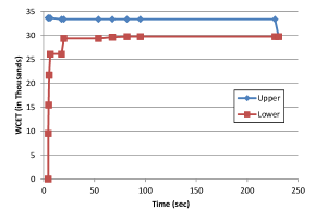
Figure 6: Progressive Upper and Lower bounds over time for diskperf

6 Related Work

The most related work is Cerny et al. [2013] which introduced the original problem of quantitative analysis over a dynamic cost model. They were the first to discuss the concept of refinement in order to eliminate spurious analysis arising from both the infeasibility of a path, as well as the in-optimality of the machine state. Their main loop iterations perform abstraction refinement in the style of the CEGAR Clarke et al. [2000] framework. The refinement strategy here is based on the notion of an extremal counterexample trace at each step, with an aim to eliminate this trace from further consideration. Our choice of refinement step shares this motivation, by choosing, in some sense, to refine the trace that maximizes the likelihood of improvement in the analysis result. The key technical difference between this work and ours is that this work refines the abstract domain, while we refine the transition system.

More specifically, we iteratively refine the Control Flow Graph (CFG) with appropriate splitting. The relationship of our refinement step to Cerny et al. [2013]’s is akin to that of Abstract Conflict Driven Clause Learning (ACDCL) D’Silva et al. [2013] to traditional CEGAR in the context of program verification. A direct tradeoff is that we need to maintain a data structure called the hybrid symbolic execution tree (HSET). But the gain is potentially significant; we quote: “ACDCL never changes the domain, and this immutability is crucial for efficiency (over CEGAR), because the implementations of the abstract domain and transformers can be highly optimized” D’Silva et al. [2013].

In the end, the algorithm of Cerny et al. [2013] is not incremental, and does not scale to the level of our benchmarks. The examples evaluated in Cerny et al. [2013] are very small and can solved easily and exactly by pre-existing algorithms such as symbolic execution. The reason for this is partly due to the nature of CEGAR whereby is it unclear how to “cache” the results of the analysis from previous iterations, let alone in a compact form. (In verification as opposed to analysis, we can cache the known safe states.) Consequently, the algorithm of Cerny et al. [2013] is not progressive: it is possible in principle to be considering the same execution path in a nonterminating sequence of refinement.

The work Cerny et al. [2015] applies the concept segment-based abstraction in Cerny et al. [2013] for high-level WCET analysis. Consequently, not only have they reached a certain level of scalability, but also their approach can be embedded effectively into the standard Implicit Path Enumeration Technique (IPET) Li and Malik [1995]. However, note importantly that in high-level WCET analysis, as opposed to overall WCET analysis, the timing of each basic block has been abstracted to the worst-case timing of the block, returned by some prior low-level analysis. Thus the problem no longer concerns a dynamic cost model. In other words, scalability is achieved partly by ignoring the issue of context-sensitivity raised by a dynamic cost model.

Another work related to ours is Beyer et al. [2008] from the BLAST Beyer et al. [2007] line of work, which dynamically adjusts the precision of the analysis. It carries an explicit analysis and an abstract analysis in the form of predicates. Then, depending on the accumulated results, for instance when the number of explicitly tracked values of a particular variable reaches a limit, the abstract domain is refined by adding a predicate and the explicit analysis is abstracted by turning it off for that variable. Our work does share a similarity with Beyer et al. [2008] in using both the exact and abstract results during analysis.

The most important difference is that their work is applied on reachability problems such as model checking and verification that are qualitative analyses, whereas we target quantitative analyses with dynamic cost model. We have demonstrated clearly that for the problem domains of interest, feasibility refinement alone is not enough.

Finally, we mention other related works, which share similar motivations as our work. Many customized abstract interpreters have been injected with some form of path-sensitivity to enhance the precision of the analysis results. A notable example is Rival and Mauborgne [2007]. There have also been work on path-sensitive algorithms (under SMT setting) equipped with abstract interpretation in order to prune (a potentially infinite number of) paths Harris et al. [2010]. However, our framework differs significantly in the way the spines are interactively constructed. On one hand, we quickly refute spurious analysis from previous iteration while computing realistic lower bounds to exploit the new concept of domination for pruning. On the other hand, we can reach early termination when the spines confirm previously computed upper bound analyses are indeed precise.

7 Concluding Remarks

We presented an algorithm for quantitative analysis defined over a dynamic cost model. The algorithm is anytime because it produces a sound analysis after every iteration of its refinement step, and is progressive because it eventually terminates with an exact analysis. Another feature is that the algorithm computes a lower and upper bound analysis thus paving the way for early termination, useful when the analysis is considered good enough according to a preset level. Finally, we show that the algorithm is incremental because it maintains a compact representation throughout the refinement steps, and each new refinement step is usually greatly assisted by the representation. We used a well-recognized benchmark from the WCET community to show that we can execute challenging examples.

References

- Banerjee et al. [2013] A. Banerjee, S. Chattopadhyay, and A. Roychoudhury. Static analysis driven cache performance testing. In RTSS, pages 319–329, 2013.
- Beyer [2014] D. Beyer. Third competition on software verification. In TACAS, 2014.
- Beyer et al. [2007] D. Beyer, T. Henzinger, R. Jhala, and R. Majumdar. The Software Model Checker BLAST. Int. J. STTT, 9:505–525, 2007.
- Beyer et al. [2008] D. Beyer, T. A. Henzinger, and G. Theoduloz. Program analysis with dynamic precision adjustment. In ASE, 2008.
- Boddy [1991] M. Boddy. Anytime problem solving using dynamic programming. In AAAI, pages 738–743, 1991.
- Cerny et al. [2013] P. Cerny, T. A. Henzinger, and A. Radhakrishna. Quantitative abstraction refinement. In POPL, pages 115–128, 2013.
- Cerny et al. [2015] P. Cerny, T. A. Henzinger, L. Kovacs, A. Radhakrishna, and J. Zwirchmayr. Segment abstraction for worst-case execution time analysis. In ESOP, pages 105–131, 2015.
- Chu and Jaffar [2011] D. H. Chu and J. Jaffar. Symbolic simulation on complicated loops for wcet path analysis. In EMSOFT, 2011.
- Cimatti et al. [2008] A. Cimatti, A. Griggio, and R. Sebastiani. Efficient interpolant generation in satisfiability modulo theories. In TACAS’08, pages 397–412, 2008.
- Clarke et al. [2000] E. Clarke, O. Grumberg, S. Jha, Y. Lu, and H. Veith. CounterExample-Guided Abstraction Refinement. In CAV, 2000.
- Craig [1955] W. Craig. Three uses of Herbrand-Gentzen theorem in relating model theory and proof theory. Journal of Symbolic Computation, 22, 1955.
- Dijkstra [1975] E. W. Dijkstra. Guarded commands, nondeterminacy and formal derivation of programs. Commun. ACM, 1975.
- D’Silva et al. [2013] V. D’Silva, L. Haller, and D. Kroening. Abstract conflict driven learning. In POPL, pages 143–154, 2013.
- Harris et al. [2010] W. R. Harris, S. Sankaranarayanan, F. Ivančić, and A. Gupta. Program analysis via satisfiability modulo path programs. In POPL, pages 71–82, 2010.
- Jaffar et al. [2008] J. Jaffar, A. E. Santosa, and R. Voicu. Efficient memoization for dynamic programming with ad-hoc constraints. In AAAI, 2008.
- Jaffar et al. [2009] J. Jaffar, A. E. Santosa, and R. Voicu. An interpolation method for CLP traversal. In 15th CP, LNCS 5732, 2009.
- Jaffar et al. [2012] J. Jaffar, V. Murali, J. Navas, and A. Santosa. Path sensitive backward analysis. In SAS, 2012.
- Li and Malik [1995] Y.-T. S. Li and S. Malik. Performance analysis of embedded software using implicit path enumeration. In DAC, 1995.
- [19] Mälardalen. Mälardalen WCET research group benchmarks. URL http://www.mrtc.mdh.se/projects/wcet/benchmarks.html, 2006.
- McMillan [2010] K. L. McMillan. Lazy annotation for program testing and verification. In CAV, 2010.
- Prantl et al. [2008] A. Prantl, M. Schordan, and J. Knoop. TuBound – a conceptually new tool for worst-case execution time analysis. In WCET, 2008.
- Puschner and Burns [2000] P. Puschner and A. Burns. A review of worst-case execution-time analysis. Journal of Real-Time Systems, 2000.
- Rival and Mauborgne [2007] X. Rival and L. Mauborgne. The trace partitioning abstract domain. ACM Trans. Program. Lang. Syst., 29(5), Aug. 2007.
- Theiling et al. [2000] H. Theiling, C. Ferdinand, and R. Wilhelm. Fast and precise WCET prediction by seperate cache and path analyses. Real-Time Systems, 18(2/3):157–179, May 2000.
- Tiwari et al. [1994] V. Tiwari, S. Malik, and A. Wolfe. Power analysis of embedded software: A first step towards software power minimization. In ICCAD, pages 384–390, 1994.
- Wilhelm et al. [2008] R. Wilhelm, J. Engblom, A. Ermedahl, N. Holsti, S. Thesing, D. Whalley, G. Bernat, C. Ferdinand, R. Heckmann, T. Mitra, F. Mueller, I. Puaut, P. Puschner, J. Staschulat, and P. Stenström. The worst-case execution-time problem—overview of methods and survey of tools. Trans. on Embedded Computing Sys., 2008.