From Collective Adaptive Systems to
Human Centric Computation and Back:
Spatial Model Checking for Medical Imaging

Abstract

Recent research on formal verification for Collective Adaptive Systems (CAS) pushed advancements in spatial and spatio-temporal model checking, and as a side result provided novel image analysis methodologies, rooted in logical methods for topological spaces. Medical Imaging (MI) is a field where such technologies show potential for ground-breaking innovation. In this position paper, we present a preliminary investigation centred on applications of spatial model checking to MI. The focus is shifted from pure logics to a mixture of logical, statistical and algorithmic approaches, driven by the logical nature intrinsic to the specification of the properties of interest in the field. As a result, novel operators are introduced, that could as well be brought back to the setting of CAS.

1 Introduction

Formal verification of properties of Collective Adaptive Systems (CAS) is a challenging subject. The huge number of considered entities introduces a gap with classical finite-state methods as the number of states grows exponentially. Approximation methods, such as mean-field or fluid-flow approximation, have been proposed to mitigate this aspect (see [6, 5, 31]). Another relevant issue is that of spatial distribution of the considered entities. Entities composing a CAS are typically located, and moving, in a physical or logical space. Collective behaviour is driven by interaction, which is frequently based on proximity. This makes spatial aspects more prominent in the case of CAS than in classical concurrent systems, and leads to the introduction of spatial properties in formal verification.

Model checking [2] is a formal verification technique that is based on static analysis of system properties that are described by modal logics. Modal operators have been traditionally used to denote possibility or necessity, probability, constraints on continuous time, access to security contexts, separation of parallel components of a system and so on. But since the very beginning, modal logics have also been interpreted on spatial structures, such as topological spaces (see [4] for a thorough introduction). In this context, formulas are interpreted as sets of points of a topological space, and in particular $\diamond\phi$ is usually interpreted as the points that lay in the closure of the interpretation of $\phi$. A standard reference is the Handbook of Spatial Logics [34]. Therein, several logics are described, with applications far beyond topological spaces; such logics treat not only aspects of morphology, geometry, distance, but also advanced topics such as dynamic systems, and discrete structures, that are particularly difficult to deal with from a topological perspective.

Model checking of spatial (and spatio-temporal) logics is a more recent development (see e.g., [16], [23], [24]). In [13], a model checking algorithm for spatial logics in the topological sense has been proposed. Therein, models are based on extensions of topological spaces called closure spaces, designed to accommodate also discrete structures such as finite graphs in the topological framework. The so-called surrounded operator is introduced to describe points that are located in a region of points satisfying a certain formula and surrounded by points satisfying another one (in other words, the surrounded operator is a spatial form of the until operator of temporal logics). The resulting logic is called SLCS (Spatial Logic of Closure Spaces). In [12], a spatio-temporal model checking algorithm using the same principles has been proposed, for a logic combining the spatial operators of SLCS with the well-known temporal operators of the Computation Tree Logic CTL. Applications to CAS have been developed in the fields of smart transportation [11], and bike-sharing systems [14]. A free and open source implementation of the spatio-temporal model checking algorithm of [12] is provided by the tool topochecker .

In this position paper, we explore various ideas for the application of spatial and spatio-temporal model checking that depart from the setting of CAS and are tailored to Human Centric Computation, in particular to the field of Medical Imaging (MI). In this domain, space consists of points called voxels, that are arranged in a multi-dimensional, possibly anisotropic grid. Several spatial analyses are performed in MI. Such analyses are typically described by structured combinations of attributes related to proximity, shape, aspect and distance of features of interest, for which spatial logics provide a well-suited descriptive language. Our work is motivated by some considerations about how medical image analysis is carried out. The overall general description of a feature (e.g. the shape and spatial arrangement of parts of an image that exhibit diseases) is often carried out informally, but in a logically structured way (e.g.: “the tumour is lighter than the surrounding brain area, and touches the oedema, whose intensity is a bit darker than the tumour”). Such description is then turned into a series of different analysis passes, sometimes performed by specific tools, but frequently done by writing ad-hoc programs. The results of such different passes are often integrated by hand or using hand-crafted scripts. This complex and elaborate process hinders the implementation, and sharing across the medical community, of novel analysis methods that emerge from current research. A leap forward is needed in the unambiguous and precise specification of such procedures, which could be provided by logical methods borrowed from Computer Science and in particular the area of formal methods. Our research program aims at paving the way and establishing foundational results for such a development to happen.

2 Spatial logics for medical imaging

The contribution of Computer Science to the field of medical image analysis is increasingly significant, and will play a key role in future healthcare. Computational methods are currently in use for several different purposes, such as: Computer-Aided Diagnosis (CAD), aiming at the classification of areas in images, based on the presence of signs of specific diseases [18]; Image Segmentation, tailored to identify areas that exhibit specific features or functions (e.g. organs or sub-structures) [21]; Automatic contouring of Organs at Risk (OAR) or target volumes (TV) for radiotherapy applications [7]; Indicators finding, that is, the identification of indicators, computed from the acquired images, that permit early diagnosis, or understanding of microscopic characteristics of specific diseases, or help in the identification of prognostic factors to predict a treatment output [10, 44]. Examples of indicators are the Mean Diffusivity and the Fractional Anisotropy obtained from Magnetic Resonance (MR) Diffusion-Weighted Images, or Magnetization Transfer Ratio maps obtained from a Magnetization Transfer acquisition [17, 32].

Such kinds of analyses are strictly related to spatial and temporal features of acquired images. For example, the diagnosis of specific diseases requires the observation of variations in time of the response to a particular acquisition technique. Another example is provided by longitudinal studies, that consist of repeated observations of the same variables over long periods of time, to help understanding the areas involved in some diseases. Such investigations can take advantage of spatial and temporal capabilities in model checking. In this work, we provide a preliminary investigation of spatial logical operators that may be used to identify areas in the images based on local or non-local features and prior knowledge (e.g., areas surrounded by or near to or similar to areas with particular properties).

We start from the spatial logic SLCS presented in [13]. SLCS features the spatial operators near and surrounded. The syntax of SLCS is defined by the following grammar, where $p$ ranges over $P$, namely the set of atomic propositions: $\Phi::=p\mid\top\mid\lnot\Phi\mid\Phi\land\Phi\mid\mathcal{N}\Phi\mid\Phi\mathcal{S}\Phi$.

In the syntax, $\top$ is the constant true; $\lnot$ and $\land$ are standard logical negation and conjunction. Formula $\mathcal{N}\phi$ denotes all points that are “near” to the interpretation of $\phi$, whereas formula $\phi_{1}\mathcal{S}\phi_{2}$ denotes all points that lie in a subset of the interpretation of $\phi_{1}$, whose “boundary” satisfies $\phi_{2}$. The notions of “near” and “boundary” are made formal in the interpretation of the logic, resorting to a closure model $((X,\mathcal{C}),v)$, where $X$ is a set, $\mathcal{C}:\mathcal{P}(X)\to\mathcal{P}(X)$ is a closure operator (see [13] for details), and $v:P\to\mathcal{P}(X)$ is the valuation of atomic propositions.

In the remainder of this paper, we discuss some additional logical operators that deal with distance (Section 3) and texture analysis (Section 4), and we reconsider the models of SLCS in the light of such additions. These operators are implemented in the experimental branch of topochecker. In models associated to medical images, $X$ is the set of points of an image, and $\mathcal{C}$ associates to each subset $A$ of $X$ the union of the neighbours of each point of $A$, by a user-defined notion of neighbourhood. To cope with the quantitative information present in medical images, atomic propositions have quantitative valuations over the real numbers, instead of just boolean valuations. However, to retain the boolean interpretation of SLCS formulas, the syntax of atomic propositions in the logic is that of constraints with variables ranging over $\mathbb{R}$. Atomic predicate $p$ is a shorthand for $p=1$. For example, formula $p>k\land q<h$ denotes all points $x\in X$ such that the value of $p$ is greater than $k$ and the value of $q$ is less than $h$. Formally, this does not require changes to SLCS and its semantics: given a set $\hat{P}$ of proposition letters, with quantitative valuation $\hat{v}:\hat{P}\to\mathbb{R}^{X}$, the set of atomic propositions $P$ is given by the set of all possible constraints on $\hat{P}$, and the valuation function $v:P\to 2^{X}$ is just evaluation of constraints, which makes use of $\hat{v}$.

3 Distance operators

Distance operators can be added to spatial logics in various ways (see [29] for an introduction). Distances are very often expressed using the real numbers $\mathbb{R}$. Typically, one considers operators of the form $\mathcal{D}^{e(z)}\phi$ where $e(z)$ is a constraint parametrised by a free variable $z$, and $\phi$ is a formula denoting a spatial property. The intended semantics is that point $x$ is a model of $\mathcal{D}^{e(z)}\phi$ if and only if there is a point $y$ satisfying $\phi$ such that the distance $d$ from $x$ to $y$ satisfies the constraint $e(d)$. Logics of metric spaces have been introduced in [30]; therein, the constraint $e(z)$ can only be in the form $z\leq k$, where $k\in\mathbb{R}$ (distance at most $k$), or $k_{1}\leq z\leq k_{2}$ (distance included between $k_{1}$ and $k_{2}$). The latter is called “doughnut operator” in [29]. Notably, the doughnut operator cannot be expressed just using $z\leq k$ in combination with boolean operators. In the following, we will discuss a general model checking procedure which is able to verify the satisfaction of such formulas in an efficient way.

Models.

First, we need to discuss appropriate models for our logics. The quasi-discrete closure models of [13] provide a starting point. A quasi-discrete closure model is completely described by a pair $(X,\mathcal{R})$ where $\mathcal{R}$ is a binary relation on a set of points $X$ – that is, a (possibly directed, unlabelled) graph – and by a valuation $v$ associating to each atomic proposition, in a finite set $P$, a set of points of $X$. This data uniquely defines a model $\mathcal{M}=((X,\mathcal{C}),v)$ where $\mathcal{C}:2^{X}\to 2^{X}$ is the closure operator, that coincides with the dilation operation of the graph $(X,\mathcal{R})$. Such models do not include information on distances. One possibility is to enrich the structure of $\mathcal{M}$ by adding a distance operator $d:X\times X\to\mathbb{R}_{\geq 0}$. In medical imaging, the structure of a metric space is a very natural setting, as typical distances are based on either Euclidean spaces or symmetric graphs. See Appendix A for more details on the possible choices for a specific metric in medical imaging applications. An open question is what are the additional axioms (one might say “compatibility conditions”) linking closure and distance. The link is well-known for the case of topological spaces. More precisely, topological spaces are obtained from metric spaces by defining open sets as those sets $S$ such that all points of $S$ have a neighbourhood in $S$; a generalization to closure spaces is an interesting topic for future research.

Distances.

In the case of quasi-discrete closure spaces generated by a graph $(X,\mathcal{R})$, it is natural to consider distance operators that are obtained by the shortest path distance of a weighted graph obtained by assigning weights to the arcs in $\mathcal{R}$. In [37], such models are used for spatial logics featuring a metric variant of the surrounded operator of [13]. Note however that in some cases other notions of distance can be more appropriate. For example, sampling an Euclidean space is often done using a regular grid, where points of a graph are arranged on multiples of a chosen unit interval, and connected by edges using some notion of connectivity (e.g. in 2-dimensional space, one typically uses four or eight neighbours per point). Shortest-path distance and Euclidean distance obviously divert in this case (see Figure 2 and Figure 3 in Appendix A), no matter how fine is the grid or how many finite neighbours are chosen. Medical images introduce some more complexity due to the fact that multi-dimensional voxels frequently are anisotropic, that is, the sizes of a voxel in each of the multiple dimensions of the image are different.

Global model checking through distance transforms.

The model checking algorithm implemented in topochecker is a global one. That is, all points of the considered space or space-time are examined, and those satisfying the considered formula are marked by the algorithm. Even though this classical approach has drawbacks – mostly related to the restriction to finite models, and the fact that large parts of a model need to be stored in central memory – it is very helpful in the case of medical image analysis, as logical operators may take advantage of global analysis of the whole space. One example where this is particularly useful is the computation of distance formulas. This can be done using so-called distance transforms. The concept of distance transform comes from the area of topology and geometry in computer vision [28]. The idea is extensively used in modern image processing. Given a multi-dimensional image equipped with Euclidean distance, global spatial model checking of formulas $\mathcal{D}^{e(z)}\phi$ can be done in linear time with respect to the number of points of the space, assuming that the computation time of $e(z)$ is negligible, and that the computation of $\phi$ is linear in turn, which is true for the spatial logic SLCS of [13]. Consider a multi-dimensional image. The outcome $S$ of computing the truth value of $\phi$ on each point of a model is a binary (multi-dimensional) image. The binary value stored in each point corresponds to the truth value of $\phi$ on that point. From this data, it is possible to define a transformed image, called the distance transform of $S$, such that in every point $x$, a value $d_{x}\in\mathbb{R}$ is stored. The value of $d_{x}$ is meant to correspond to the minimum distance between $x$ and a point satisfying $\phi$. There exist both exact and approximate algorithms for computing distance transforms, that are usually classified by their asymptotic complexity, computational efficiency, and possibility of parallel execution. In particular, there are effective linear-time algorithms [35, 19]. In global model checking, one first computes the distance transform, and then in one pass, for each $x$, the quantitative value of $d_{x}$ can be replaced with the boolean value of $e(d_{x})$. It is worth noting that similar algorithms exist for weighted graphs equipped with shortest-path distance. In this case, asymptotic complexity is generally speaking quasi-linear but not linear, although execution time is highly dependent on the structure of the considered graph.

In the next section we shall discuss how distance operators can be combined with texture analysis to identify tissues of different nature that lay within a certain distance of each other.

4 Texture analysis operators

Texture analysis (TA) operators are designed for finding and analysing patterns in medical images, including some that are imperceptible to the human visual system. Patterns in images are entities characterised by brightness, colour, shape, size, etc. TA includes several techniques and has proved promising in a large number of applications in the field of medical imaging [27, 33, 8, 15]; in particular it has been used in CAD applications [45, 25, 26] and for classification or segmentation of tissues or organs [9, 40, 39]. In TA, image textures are usually characterised by estimating some descriptors in terms of quantitative features. Typically, such features fall into three general categories: syntactic, statistical, and spectral [27]. Our preliminary experiments have been mostly focused on statistical approaches to texture analysis. Statistical methods consist of extracting a set of statistics descriptors from the distributions of local features at each voxel. In particular, we studied first order statistical methods, that are statistics based on the probability density function of the intensity values of the voxels of parts, or the whole, of an image, approximated as a histogram collecting such values into batches (driven by ranges). In this approach, the specific pixel adjacency relationship is not taken into account. Common features are statistical indicators such as mean, variance, skewness, kurtosis, entropy [41]. Although a limitation of these operators is that they ignore the relative spatial placement of voxels, statistical operators are important for MI as their application is invariant under transformations of the image. In particular, first order operators are, by construction, invariant under affine transformations (rotation and scaling), which is necessary when analysing several images acquired in different conditions. Nevertheless it is possible to construct features using first order operators, keeping some spatial coherence but losing at least partially the aforementioned invariance [43].

In our experimental evaluation, we defined a logical operator, called SCMP – for statistical comparison – that compares areas of an image that are statistically similar to a predetermined area $SA$, identified using a sub-formula. More precisely, SCMP is used to search for sub-areas in the image whose empirical distribution is similar to that of $SA$, up-to a user-specified threshold. For each voxel, a small surrounding area is considered; its statistical distribution is compared to that of $SA$ and a threshold is applied, obtaining a Boolean value that denotes whether the voxel belongs to an area statistically similar to $SA$. Statistical distributions are compared using the cross-correlation function. Currently, the syntax and interpretation of the operator are quite experimental, and different methods may be used to define the data aggregation and comparison of distributions which are needed for its implementation. Complexity is, among others, an issue to deal with.

The SCMP operator results in a generalisation of classical TA based on first-order statistics, since it analyses the statistical distribution of a neighbourhood of each voxel as a whole, whereas classical techniques for TA resort to the extraction of specific indicators. In Figure 1 we show the output of topochecker, enhanced with the SCMP operator, and the distance-based operators described in Section 3, applied to a slice of a MR-Flair acquisition of a brain affected by glioblastoma (GBM), an intracranial neoplasm. GBMs are tumors composed of typically poorly-marginated, diffusely infiltrating necrotic masses. Even if the tumor is totally resected, it usually recurs, either near the original site, or at more distant locations within the brain. GBMs are localised to the cerebral hemispheres and grow quickly to various sizes, from only a few centimetres, to lesions that cover a whole hemisphere. Infiltration beyond the visible tumor margin is always present. In MR T2/Flair images GBMs appear hyperintense and surrounded by vasogenic oedema.

Being able to segment tumor and oedema in medical images can be of immediate use for automatic contouring applications in radiotherapy and, in perspective, it can be helpful in detecting the invisible infiltrations in CAD applications. In 1(b) we show a segmentation obtained using topochecker. First, two thresholds are applied to the original image, in order to identify two areas of the image with particular brightness, that are supposed to loosely correspond to an oedema and a tumor. Furthermore, the distance operator (shortest path distance with 9-neighbours, see Appendix A) is used to imposes a certain degree of proximity between the oedema and the tumor. The voxels assigned to the oedema are drawn in yellow; the voxels assigned to tumor are drawn in orange. These areas are used as two different $SA$ for the analysis shown in 1(c), obtained using the SCMP operator to further enlarge the two regions, by searching areas that, although not falling in the specified thresholds, are still identifiable as oedema and tumor. The model checker colours the additional voxels assigned to tumor in blue; these areas are characterised by a statistical distribution similar to the orange region. The tool colours the additional voxels assigned to oedema in magenta. These are obtained by searching for areas having statistical distribution similar to the yellow part of the image. In 1(d) we show the final result of the procedure with tumor voxels in orange and oedema voxels in yellow.

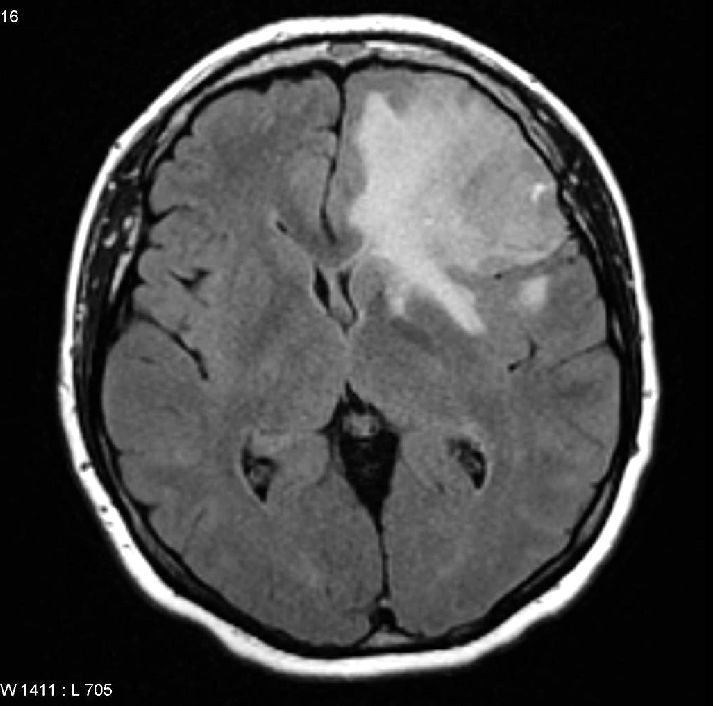
(a) A slice of a FLAIR MR acquisition of a brain affected by a glioblastoma. Same slice superimposed to regions of interest (ROIs) determined by threshold and distance operator. The yellow ROI is the oedema and the orange is the tumor.      

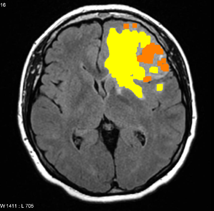
(b) Same slice superimposed to regions of interest (ROIs) determined by threshold and distance operator. The yellow ROI is the oedema; the orange one is the tumor.

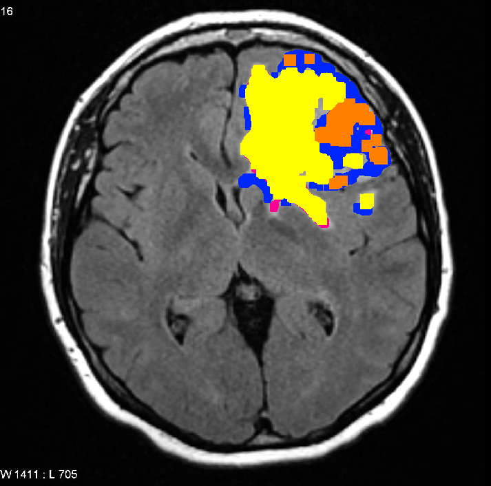
(c) Same slice superimposed to ROIs determined by the SCMP operator, starting from orange and yellow ROIs. In blue, the additional tumor voxels; in magenta, the additional oedema voxels.

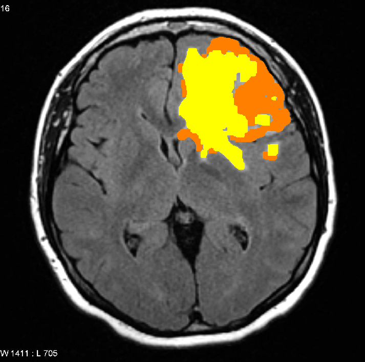
(d) Final result of application of threshold, distance, and the SCMP operator. The yellow area is the identified oedema; the orange area is the tumor. Same slice superimposed to ROIs determined by the SCMP operator. Blue are the tumor voxels and magenta the oedema voxels identified by SCMP starting from orange and yellow ROIs respectively.

Figure 1: Experimental results obtained by applying topochecker to a medical image of a brain (case courtesy of A.Prof Frank Gaillard, Radiopaedia.org, rID: 5292).

5 Discussion

We have just started the exploration of logical methods for medical image analysis in the domain of radiotherapy. Logical properties are used as classifiers for points of an image; this can be used both for colouring regions that may be similar to diseased tissues, and therefore being diseased tissue in turn, and for colouring regions corresponding to organs of the human body. Envisaged applications range from contouring to computer-aided diagnosis. The field of Spatial Logics can benefit from such kinds of research; for example, texture analysis operators may be defined, and in particular operators that compare regions based on statistical similarity. It will be interesting to study relevant axioms and theories that can deal with the uncertainty generated by analysis of statistical similarity in theorem proving or completeness studies, as well as theories of bisimilarity or minimisation of models. From the model-theoretical point of view, questions of interest relate to the various kinds of distances that may arise in the considered spatial models, ranging from classical Euclidean distance to shortest-path distance on weighted graphs, on their axioms, and the relation between different notions. The effect of approximate distance transforms on the representational complexity of models may be an interesting question for future work. Our early experiments show that typical analyses carried out using spatial model checking in medical imaging require careful calibration of numeric parameters (for example, a threshold for the distance between a tumor and the associated oedema, or the size of areas identified by a formula, that are small enough to be considered noise, and ought be filtered out). The calibration of such parameters can be done using machine-learning techniques. In this respect, future work could be focused on application, in the context of our research line, of the methodology developed by Bartocci et al. (see e.g. [20, 3]). Some recent research focused on themes that are close to our planned development. In particular, [42] uses spatio-temporal model checking techniques inspired by [23] – pursuing machine learning of the logical structure of image features – to the detection of tumors. In contrast, our approach is more focused on human-intelligible logical descriptions. The work [38] is closer to the setting of CAS, applied to biological processes, with an interesting focus on multi-scale aspects. The research line that we present in this paper stems from research in collective adaptive systems and departs from it to direct spatial analysis to medical imaging. We foresee that the novel statistical texture analysis operators and the study of global model checking of distance formulas using distance transforms are of interest when dealing with very large populations that are spread over some spatial structure (e.g. a geographical map). Potential applications include the analysis of statistical properties arising from gossip protocols and disease spreading models, in which statistical distribution of features in space appears to be relevant.

Acknowledgements

The authors wish to thank Marco Di Benedetto for suggesting the application of distance transforms to improve the complexity of model checking of formulas with distances, and the Medical Physics department of Azienda Ospedaliera Universitaria Senese (director: Fabrizio Banci Buonamici) for institutional support and encouragement in this research program.

Appendix A Comparison of metrics

In MI, Euclidean distance (based on the 2-norm) is the reference distance between two voxels. Therefore, in this context, Euclidean distance is considered error-free. We shall now discuss different alternative definitions of distance that could be interesting for spatial model checking, both for medical imaging applications and also as a valuable addition to spatial analysis methods for CAS. Starting from [22], we experimented with two distance transform operators, the multi-dimensional Euclidean error-free distance operator, called EUCL in the following, and a distance transform operator based on Dijkstra’s shortest path algorithm, called MDDT (Modified Dijkstra Distance Transform), that operates on the shortest-path distance of a graph constructed from the image. From the point of view of the Dijkstra algorithm, an image is a graph whose vertices are the voxels and whose arcs connect each voxel $x$ with chosen voxels that are considered adjacent to $x$. Every arc is labelled with the chosen distance function applied to the two vertices that the arc connects. In other words, we are considering a graph with nodes located in a distance space, arcs weighted according to the distance of the space, and a chosen notion of adjacency. In this particular case, the shortest-path distance is also called Chamfer distance. The chosen adjacency is the most important factor in the precision-efficiency trade-off of the computed distance: the more adjacent voxels are considered, the more precise is the Chamfer distance when compared to the Euclidean distance, at the expenses of generating graphs with larger out-degrees. In Figure 2 and Figure 3 we show in red the points satisfying $\mathcal{D}^{z>k}\phi$ for a binary image with only one point satisfying $\phi$ (in the centre of the image). In Figure 2 we show the output of the error-free EUCL operator. In Figure 3, we show the output of the MDDT operator, alongside the characteristic pattern of the percentage error with respect to Euclidean distance (3(b) and 3(d) – see [22] for a detailed analysis of the percentage error of several distance transform algorithms). The percentage error $\delta(x)$ for the distance transform $d(x)$ is defined in every voxel $x$ as $\delta(x)=\frac{\left|d_{eucl}(x)-d(x)\right|}{d_{eucl}(x)}$. In 3(a) and 3(c) we show the Chamfer distance obtained using MDDT, with different choices of adjacent voxels. In 3(a) the adjacent voxels of a point are chosen to be its immediate neighbours on the main directions and diagonals (called Moore neighbourhood in 2d images). In 3(c), again the main directions and diagonals are used, but this process is iterated two times (that is, the chosen adjacent voxels of $x$ are all points in a hypercube of size 5, centred on $x$, except $x$ itself).

Figure 2: Error-free Euclidean distance (with threshold) from a point in the centre of image.

(a) Chamfer distance in two dimensions with the Moore neighbourhood

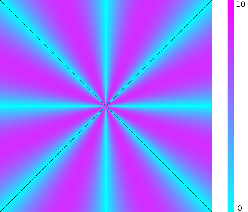
(b) Percentage error with respect to the error-free Euclidean distance. Scale: 0-10%

(c) Chamfer distance in two dimensions with 24 chosen adjacent voxels.

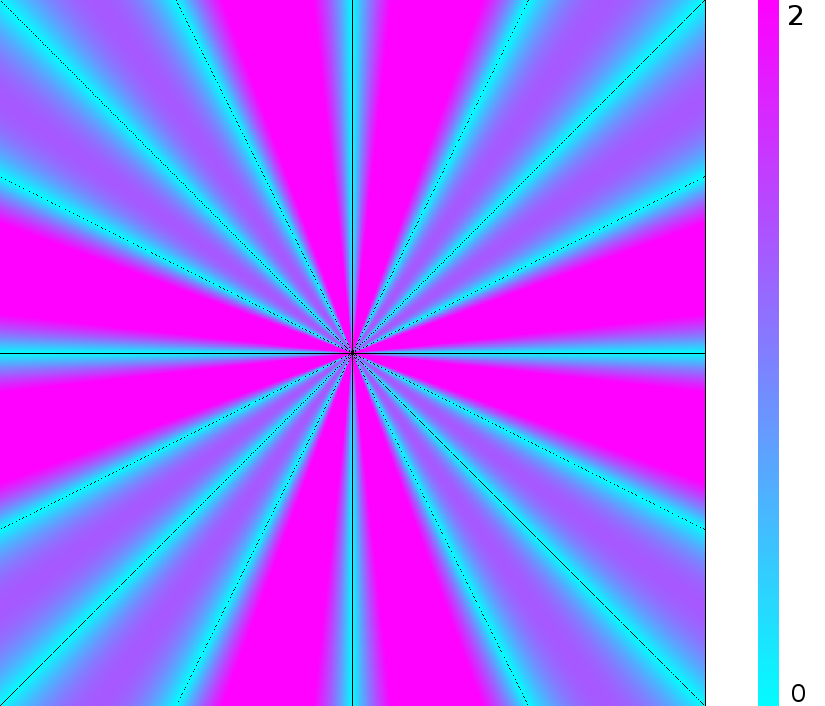
(d) Percentage error with respect to the error-free Euclidean distance. Scale: 0-2%

Figure 3: Distance operators, from the central point, with a threshold.

In a Euclidean space, Euclidean distance is not the only possible distance; several definitions exist based on different norms. In (Figure 4) we depict two widely used metrics. In 4(a) adjacency is the same as in 3(a) but all arcs have weight 1. This is called the Chebyshev or chessboard distance, that in a Euclidean space is the distance based on the so-called infinity-norm. In 4(b), the underlying graph is as in 4(a) but adjacency contains only voxels whose coordinates differ at most in one dimension) (for 2D images, this is called Von Neumann neighbourhood), thus obtaining the taxicab or cityblock distance. In a Euclidean space, the cityblock distance is the distance based on 1-norm.

(a) Chessboard distance: $d_{\infty}(x,y)=\max_{i}{\left|x_{i}-y_{i}\right|}$

(b) CityBlock distance: $d_{1}(x,y)=\sum_{i}{\left|x_{i}-y_{i}\right|}$ aaa

Figure 4: Non-Euclidean distance defined in an Euclidean space.

References

- [1]
- [2] C. Baier & J. Katoen (2008): Principles of model checking. MIT Press.
- [3] E. Bartocci, L. Bortolussi, D. Milios, L. Nenzi & G. Sanguinetti (2015): Studying Emergent Behaviours in Morphogenesis Using Signal Spatio-Temporal Logic, pp. 156–172. Springer, 10.1007/978-3-319-26916-0_9.
- [4] J. van Benthem & G. Bezhanishvili (2007): Modal Logics of Space. In: Handbook of Spatial Logics, Springer, pp. 217–298, 10.1007/978-1-4020-5587-4_5.
- [5] L. Bortolussi, J. Hillston, Latella. D. & M. Massink (2013): Continuous approximation of collective system behaviour: A tutorial. Perform. Eval. 70(5), pp. 317–349, 10.1016/j.peva.2013.01.001.
- [6] Luca Bortolussi & Jane Hillston (2012): Fluid Model Checking. In: CONCUR 2012 - Concurrency Theory - 23rd International Conference, Lecture Notes in Computer Science 7454, Springer, pp. 333–347, 10.1007/978-3-642-32940-1_24.
- [7] K.K. Brock (2014): Image processing in radiation therapy. CRC Press, 10.1118/1.4905156.
- [8] G. Castellano, L. Bonilha, L.M. Li & F. Cendes (2004): Texture analysis of medical images. Clinical Radiology 59(12), pp. 1061–1069, 10.1016/j.crad.2004.07.008.
- [9] C.-C. Chen, J.S. DaPonte & M.D. Fox (1989): Fractal feature analysis and classification in medical imaging. IEEE Transactions on Medical Imaging 8(2), pp. 133–142, 10.1109/42.24861.
- [10] G. Chetelat & J. Baron (2003): Early diagnosis of alzheimer’s disease: contribution of structural neuroimaging. NeuroImage 18(2), pp. 525–541, 10.1016/S1053-8119(02)00026-5.
- [11] V. Ciancia, S. Gilmore, D. Latella, M. Loreti & M. Massink (2014): Data Verification for Collective Adaptive Systems: Spatial Model-Checking of Vehicle Location Data. In: Eighth IEEE International Conference on Self-Adaptive and Self-Organizing Systems Workshops, SASOW, IEEE Computer Society, pp. 32–37, 10.1109/SASOW.2014.16.
- [12] V. Ciancia, G. Grilletti, D. Latella, M. Loreti & M. Massink (2015): An Experimental Spatio-Temporal Model Checker. In: Software Engineering and Formal Methods - SEFM 2015 Collocated Workshops, Lecture Notes in Computer Science 9509, Springer, pp. 297–311, 10.1007/978-3-662-49224-6_24.
- [13] V. Ciancia, D. Latella, M. Loreti & M. Massink (2014): Specifying and Verifying Properties of Space. In: Theoretical Computer Science - 8th IFIP TC 1/WG 2.2 International Conference, TCS 2014, Rome, Italy, September 1-3, 2014. Proceedings, Lecture Notes in Computer Science 8705, Springer, pp. 222–235, 10.1007/978-3-662-44602-7_18.
- [14] V. Ciancia, D. Latella, M. Massink & R. Pakauskas (2015): Exploring Spatio-temporal Properties of Bike-Sharing Systems. In: 2015 IEEE International Conference on Self-Adaptive and Self-Organizing Systems Workshops, SASO Workshops, IEEE Computer Society, pp. 74–79, 10.1109/SASOW.2015.17.
- [15] F. Davnall, C. S. P. Yip, G. Ljungqvist, M. Selmi, F. Ng, B. Sanghera, B. Ganeshan, K. A. Miles, G. J. Cook & V. Goh (2012): Assessment of tumor heterogeneity: an emerging imaging tool for clinical practice? Insights into Imaging 3(6), pp. 573–589, 10.1007/s13244-012-0196-6.
- [16] R. De Nicola, J. Katoen, D. Latella, M.. Loreti & M. Massink (2007): Model checking mobile stochastic logic. Theor. Comput. Sci. 382(1), pp. 42–70, 10.1016/j.tcs.2007.05.008.
- [17] S. De Santis, M. Drakesmith, S. Bells, Y. Assaf & D. K. Jones (2014): Why diffusion tensor MRI does well only some of the time: Variance and covariance of white matter tissue microstructure attributes in the living human brain. NeuroImage 89, pp. 35–44, 10.1016/j.neuroimage.2013.12.003.
- [18] Kunio Doi (2007): Computer-aided diagnosis in medical imaging: Historical review, current status and future potential. Comput. Med. Imaging Graph. 31(4-5), pp. 198–211, 10.1016/j.compmedimag.2007.02.002.
- [19] R. Fabbri, L. Da Fontoura Da Costa, J. C. Torelli & O. M. Bruno (2008): 2D Euclidean Distance Transform Algorithms: A Comparative Survey. ACM Comput. Surv. 40(1), pp. 2:1–2:44, 10.1145/1322432.1322434.
- [20] E.A. Gol, E. Bartocci & C. Belta (2014): A formal methods approach to pattern synthesis in reaction diffusion systems. In: 53rd IEEE Conference on Decision and Control, pp. 108–113, 10.1109/CDC.2014.7039367.
- [21] N. Gordillo, E. Montseny & E. Sobrevilla (2013): State of the art survey on MRI brain tumor segmentation. Magn. Reson. Imaging. 31(8), pp. 1426–1438, 10.1016/j.mri.2013.05.002.
- [22] G. J. Grevera (2007): Distance Transform Algorithms And Their Implementation And Evaluation. In: Deformable Models, Springer Science, pp. 33–60, 10.1007/978-0-387-68413-0_2.
- [23] R. Grosu, S.A. Smolka, F. Corradini, A. Wasilewska, E. Entcheva & E. Bartocci (2009): Learning and detecting emergent behavior in networks of cardiac myocytes. Commun. ACM 52(3), pp. 97–105, 10.1145/1467247.1467271.
- [24] I. Haghighi, A. Jones, Z. Kong, E. Bartocci, R. Grosu & C. Belta (2015): SpaTeL: A Novel Spatial-temporal Logic and Its Applications to Networked Systems. In: Proceedings of the 18th International Conference on Hybrid Systems: Computation and Control, HSCC ’15, ACM, New York, NY, USA, pp. 189–198, 10.1145/2728606.2728633.
- [25] F. Han, H. Wang, G. Zhang, H. Han, B. Song, L. Li, W. Moore, H. Lu, H. Zhao & Z. Liang (2014): Texture Feature Analysis for Computer-Aided Diagnosis on Pulmonary Nodules. Journal of Digital Imaging 28(1), pp. 99–115, 10.1007/s10278-014-9718-8.
- [26] T. Heinonen, T. Arola, A. Kalliokoski, P. Dastidar, M. Rossi, S. Soimakallio, J. Hyttinen & H. Eskola (2009): Computer Aided Diagnosis Tool for the Segmentation and Texture Analysis of Medical Images. In: IFMBE Proceedings, Springer Science, pp. 274–276, 10.1007/978-3-642-03879-2_77.
- [27] A. Kassner & R. E. Thornhill (2010): Texture Analysis: A Review of Neurologic MR Imaging Applications. Am. J. Neuroradiol. 31(5), pp. 809–816, 10.3174/ajnr.A2061.
- [28] R. Kimmel, N. Kiryati & A. M. Bruckstein (1996): Sub-pixel distance maps and weighted distance transforms. Journal of Mathematical Imaging and Vision 6(2), pp. 223–233, 10.1007/BF00119840.
- [29] R. Kontchakov, A. Kurucz, F. Wolter & M. Zakharyaschev (2007): Spatial Logic + Temporal Logic = ? In: Handbook of Spatial Logics, Springer, pp. 497–564, 10.1007/978-1-4020-5587-4_9.
- [30] O. Kutz, F. Wolter, H. Sturm, N. Suzuki & M. Zakharyaschev (2003): Logics of metric spaces. ACM Trans. Comput. Log. 4(2), pp. 260–294, 10.1145/635499.635504.
- [31] D. Latella, M. Loreti & M. Massink (2015): On-the-fly PCTL fast mean-field approximated model-checking for self-organising coordination. Science of Computer Programming 110, pp. 23 – 50, 10.1016/j.scico.2015.06.009.
- [32] C. Li, J. G. Herndon, F. J. Novembre & X. Zhang (2015): A Longitudinal Magnetization Transfer Imaging Evaluation of Brain Injury in a Macaque Model of NeuroAIDS. AIDS Research and Human Retroviruses 31(3), pp. 335–341, 10.1089/aid.2014.0166.
- [33] R. Lopes, A. Ayache, N. Makni, P. Puech, A. Villers, S. Mordon & N. Betrouni (2011): Prostate cancer characterization on MR images using fractal features. Med. Phys. 38(1), p. 83, 10.1118/1.3521470.
- [34] Aiello M., Pratt-Hartmann I. & van Benthem J., editors (2007): Handbook of Spatial Logics. Springer, 10.1007/978-1-4020-5587-4.
- [35] C.R. Maurer, Rensheng Qi & V. Raghavan (2003): A linear time algorithm for computing exact Euclidean distance transforms of binary images in arbitrary dimensions. IEEE Transactions on Pattern Analysis and Machine Intelligence 25(2), pp. 265–270, 10.1109/TPAMI.2003.1177156.
- [36] L. Nenzi & L. Bortolussi (2014): Specifying and Monitoring Properties of Stochastic Spatio-Temporal Systems in Signal Temporal Logic. In: 8th International Conference on Performance Evaluation Methodologies and Tools, VALUETOOLS 2014, Bratislava, Slovakia, December 9-11, 2014, ICST, 10.4108/icst.valuetools.2014.258183.
- [37] L. Nenzi, L. Bortolussi, V. Ciancia, M. Loreti & M. Massink (2015): Qualitative and Quantitative Monitoring of Spatio-Temporal Properties. In: Runtime Verification - 6th International Conference, RV 2015 Vienna, Austria, September 22-25, 2015. Proceedings, Lecture Notes in Computer Science 9333, Springer, pp. 21–37, 10.1007/978-3-319-23820-3_2.
- [38] O. Pârvu & D. Gilbert (2016): A Novel Method to Verify Multilevel Computational Models of Biological Systems Using Multiscale Spatio-Temporal Meta Model Checking. PLoS ONE 11(5), pp. 1–43, 10.1371/journal.pone.0154847.
- [39] D. Rodriguez Gutierrez, A. Awwad, L. Meijer, M. Manita, T. Jaspan, R. A. Dineen, R. G. Grundy & D. P. Auer (2013): Metrics and Textural Features of MRI Diffusion to Improve Classification of Pediatric Posterior Fossa Tumors. American Journal of Neuroradiology 35(5), pp. 1009–1015, 10.3174/ajnr.A3784.
- [40] N. Sharma, A. Ray, S. Sharma, K.K. Shukla, S. Pradhan & L. Aggarwal (2008): Segmentation and classification of medical images using texture-primitive features: Application of BAM-type artificial neural network. J Med Phys 33(3), p. 119, 10.4103/0971-6203.42763.
- [41] G.N. Srinivasan & G. Shobha (2012): Statistical Texture Analysis. In: Proceedings of World Accademy of Science, Engineering and Technology, 36, pp. 1264–1269.
- [42] A. Sundstrom, E. Grabocka, D. Bar-Sagi & B. Mishra (2016): Histological Image Processing Features Induce a Quantitative Characterization of Chronic Tumor Hypoxia. PLoS ONE 11(4), pp. 1–30, 10.1371/journal.pone.0153623.
- [43] B. M. Tijms, P. Series, D. J. Willshaw & S. M. Lawrie (2011): Similarity-Based Extraction of Individual Networks from Gray Matter MRI Scans. Cerebral Cortex 22(7), pp. 1530–1541, 10.1093/cercor/bhr221.
- [44] A. T. Toosy (2003): Diffusion tensor imaging detects corticospinal tract involvement at multiple levels in amyotrophic lateral sclerosis. J. Neurol. Neurosurg. Psychiatry 74(9), pp. 1250–1257, 10.1136/jnnp.74.9.1250.
- [45] B.J. Woods, B. D. Clymer, T. Kurc, J. T. Heverhagen, R. Stevens, Orsdemir A., O. Bulan & M. V. Knopp (2007): Malignant-lesion segmentation using 4D co-occurrence texture analysis applied to dynamic contrast-enhanced magnetic resonance breast image data. J. Magn. Reson. Imaging 25(3), pp. 495–501, 10.1002/jmri.20837.