Search for continuous gravitational waves from neutron stars in globular cluster NGC 6544

Abstract

We describe a directed search for continuous gravitational waves in data from the sixth initial LIGO science run. The target was the nearby globular cluster NGC 6544 at a distance of $\approx 2.7$ kpc. The search covered a broad band of frequencies along with first and second frequency derivatives for a fixed sky position. The search coherently integrated data from the two LIGO interferometers over a time span of 9.2 days using the matched-filtering $\mathcal{F}$-statistic. We found no gravitational-wave signals and set 95% confidence upper limits as stringent as $6.0\times 10^{-25}$ on intrinsic strain and $8.5\times 10^{-6}$ on fiducial ellipticity. These values beat the indirect limits from energy conservation for stars with characteristic spindown ages older than 300 years and are within the range of theoretical predictions for possible neutron-star ellipticities. An important feature of this search was use of a barycentric resampling algorithm which substantially reduced computational cost; this method will be used extensively in searches of Advanced LIGO and Virgo detector data.

I Introduction

The LIGO Scientific Collaboration (LSC) and Virgo Collaboration have undertaken numerous searches for continuous gravitational waves (GW). None has yet detected a signal, but many have placed interesting upper limits on possible sources. These searches have generally been drawn from one of three types.

Targeted searches are aimed at a single known pulsar, with a known precise timing solution. The first search for continuous waves, using data from the first initial LIGO science run (S1), was of this type S1pulsar , and subsequent searches have probed the Crab and Vela pulsars, among others S2pulsars ; S3S4pulsars ; S5Crab ; VirgoVela ; S5pulsars ; S6pulsars . A number of these most recent searches have been able to set direct upper limits on GW emission comparable to or stricter than the indirect “spin-down limits” (derived from energy conservation, as well as the distance from Earth of the target, its gravitational-wave frequency, and the frequency’s first derivative, the “spin-down”) for a few of the pulsars searched.

All-sky searches, as their name suggests, survey the entire sky for neutron stars not seen as pulsars. These are very computationally costly, searching over wide frequency bands and covering large ranges of spin-down parameters S2Hough ; S2Fstat ; S4PSH ; S4Einstein ; S5PowerFlux ; S5Einstein ; S5PowerFlux2 ; S5Einstein2 ; S5Hough ; VirgoAllSky . The latest of these have incorporated new techniques to cover possible binary parameters as well AllSkyBinary . Recent all-sky searches have set direct upper limits close to indirect upper limits derived from galactic neutron-star population simulations KnispelAllen .

Directed searches sit between these two extremes. As in the all-sky case, their targets are neutron stars not seen as pulsars, so that the frequency and other parameters are unknown. They focus, however, on a known sky location (and therefore a known detector-frame Doppler modulation). This directionality allows for searching over a wide range of frequencies and frequency derivatives while remaining much cheaper computationally than an all-sky search without sacrificing sensitivity. This approach was first used in a search for the accreting neutron star in the low-mass X-ray binary Sco X-1 S2Fstat ; S4radiometer ; S5Stochastic .

The search for the central compact object (CCO) in the supernova remnant (SNR) Cassiopeia A (Cas A)S5CasA was the first directed search for a young neutron star without electromagnetically detected pulsation, motivated by the idea that young neutron stars might be promising emitters of continuous GW. The Cas A search S5CasA set upper limits on GW strain which beat an indirect limit derived from energy conservation and the age of the remnant Wette2008 over a wide frequency band. Other directed searches have since followed in its footsteps, using different data analysis methods, for supernova 1987A and unseen neutron stars near the galactic center S5Stochastic ; S5GalacticCenter . Most methodologically similar to this search and the S5 Cas A search was a recent search for nine supernova remnants S6CasAFriends , which also used fully coherent integration over observation times on the order of 10 days.

In this article, we describe a search of data from the sixth initial LIGO science run (S6) for potential young isolated neutron stars with no observed electromagnetic pulsations in the nearby ($d\approx 2.7$ kpc) globular cluster NGC 6544. Globular clusters are unlikely to contain young neutron stars, but in these dense environments older neutron stars may be subject to debris accretion (see Sec. II.3) or other events which could render them detectable as gravitational wave sources. This particular globular cluster was chosen so that a computationally-feasible coherent search similar to S5CasA could beat the age-based indirect limits on GW emission.

The search did not find a GW signal, and hence the main result is a set of upper limits on strain amplitude, fiducial ellipticity, and $r$-mode amplitude $\alpha$, similar to those presented in S5CasA . An important new feature of the search described here was use of a barycentric resampling algorithm which substantially reduced computational cost, allowing a search over a larger parameter space using a longer coherence time (see Sec. II.4). This barycentric resampling method will be used extensively in searches of Advanced LIGO and Virgo detector data.

This article is structured as follows: In Sec. II we present the method, implementation, and results of the search. The upper limits set in the absence of a signal are presented in Sec. III, and the results are discussed in Sec. IV.

II Searches

II.1 Data selection

The sixth initial LIGO science run (S6) extended from July 7 2009 21:00:00 UTC (GPS 931035615) to October 21 2010 00:00:00 UTC (GPS 971654415) and included two initial LIGO detectors with 4-km arm lengths, H1 at LIGO Hanford Observatory (LHO) near Hanford, Washington and L1 at LIGO Livingston Observatory (LLO) near Livingston, Louisiana.

After optimization at fixed computing cost determined an optimum coherence time of 9.2 days (see Sec. II.4), two different methods were used to determine which data would be searched, producing two different 9.2-day stretches. Both were searched, allowing for the comparison of search results between them.

The first method was to look for the most sensitive average data from S6. This was done by taking nine week-long data samples from each detector spaced roughly 55 days apart, giving nine evenly spaced weeks throughout the duration of S6. The data samples used are shown in Table  1. We chose four representative frequencies ($100$ Hz, $200$ Hz, $400$ Hz, $600$ Hz) and generated joint-detector strain noise power spectral densities (PSDs) in $1$-Hz bands about these frequencies, using $0.01$-Hz binning. The sensitivity $h_{\textup{sens}}$ was then taken to be

$$h_{\textup{sens}}^{j}=\left(\frac{1}{\sqrt{(1/100)\cdot\sum_{i=0}^{100}(S_{h}^{i}(f_{i}))^{-1}}}\right)_{j}$$ (1)

where $S_{h}^{i}(f)$ represents the PSD value of the $i^{th}$ bin, at frequency $f_{i}$, and the index $j$ runs from 1 through 4 and represents the four representative frequencies (note that this is not an actual estimate of detectable strain). Based on this figure of merit, the final nine days of S6 yielded the most sensitive data stretch for all four frequencies: October 11-20, 2010 (GPS 970840605 – 971621841).

S6 sampling times
Label	GPS Start	GPS End	Dates (UTC)
Week 1	931053000	931657800	Jul 8-15, 2009
Week 2	936053000	936657800	Sep 3-10, 2009
Week 3	941053000	941657800	Oct 31-Nov 7, 2009
Week 4	946053000	946657800	Dec 28, 2009-Jan 4, 2010
Week 5	951053000	951657800	Feb 24-Mar 3, 2010
Week 6	956053000	956657800	Apr 23-30, 2010
Week 7	961053000	961657800	Jun 20-27, 2010
Week 8	966053000	966657800	Aug 17-24, 2010
Week 9	971053000	971657800	Oct 14-21, 2010

Table 1: The weeks sampled to find the most sensitive S6 data. Times are given both in GPS and UTC calendar dates.

An alternate data selection scheme S6CasAFriends ; S5CasA , which takes detector duty cycle into account is to maximize the figure of merit

$$\sum_{k,f}\frac{1}{S_{h}(f)}$$ (2)

where $S_{h}(f)$ represents the strain noise power spectral density at frequency $f$ in the $k^{th}$ Short Fourier Transform (SFT), and the sum is taken across all frequencies $f$ in the search band and all SFTs in a given 9.2-day (see Sec. II.4 below) observation time. The SFT format is science-mode detector data split into 1800s segments, band-pass filtered from 40–2035 Hz, Tukey windowed in the time domain, and Fourier transformed. This method favored a different data stretch: July 24–August 2, 2010 (GPS 964007133 – 964803598). This second data stretch had slightly worse average sensitivity than the first, but a higher detector livetime: our first (October) data set contained 374 SFTs (202 from Hanford and 172 from Livingston) with average sensitivity $h_{sens}^{200\textup{Hz}}=1.92\times 10^{-23}$; the second (July-August) data set contained 642 SFTs (368 from Hanford and 274 from Livingston) with average sensitivity $h_{sens}^{200\textup{Hz}}=1.95\times 10^{-23}$.

II.2 Analysis method

The analysis was based on matched filtering, the optimal method for detecting signals of known functional form. To obtain that form we assumed that the potential target neutron star did not glitch (suffer an abrupt frequency jump) or have significant timing noise (additional, possibly stochastic, time dependence of the frequency) LyneSmith2006 during the observation. We also neglected third and higher derivatives of the GW frequency, based on the time span and range of $\dot{f}$ and $\ddot{f}$ (the first two derivatives) covered. The precise expression for the interferometer strain response $h(t)$ to an incoming continuous GW also includes amplitude and phase modulation by the changing of the beam patterns as the interferometer rotates with the earth. It depends on the source’s sky location and orientation angles, as well as on the parameters of the interferometer. The full expression can be found in Jaranowski1998 .

The detection statistic used was the multi-interferometer $\mathcal{F}$-statistic Cutler2005 , based on the single-interferometer $\mathcal{F}$-statistic Jaranowski1998 . This combines the results of matched filters for the signal in a way that is computationally fast and nearly optimal Prix2009 . Assuming Gaussian noise, $2\mathcal{F}$ is drawn from a $\chi^{2}$ distribution with four degrees of freedom.

We used the implementation of the $\mathcal{F}$-statistic in the LALSuite package lalsuite . In particular most of the computing power of the search was spent in the ComputeFStatistic_v2 program. Unlike the version used in preceding methodologically similar searches S5CasA ; S6CasAFriends , this one implements an option to use a barycentric resampling algorithm which significantly speeds up the analysis.

The method of efficiently computing the $\mathcal{F}$-statistic by barycentering and Fast-Fourier-transforming the data was first proposed in Jaranowski1998 . Various implementations of this method have been developed and used in previous searches, such as Krolak2010 ; PinkeshMethods ; PatelThesis . Here we are using a new LALSuite lalsuite implementation of this method, which evolved out of PatelThesis , and which will be described in more detail in a future publication. It converts the input data into a heterodyned, downsampled timeseries weighted by antenna-pattern coefficients, and then resamples this timeseries at the solar system barycenter using an interpolation technique. The resampled time series is then Fourier-transformed to return to the frequency domain, and from there the $\mathcal{F}$-statistic is calculated. For this search, both single-detector and multi-detector $\mathcal{F}$-statistics were calculated (see Vetoes section below).

Timing tests run on a modern processor (ca. 2011) showed that the resampling code was more than 24 times faster in terms of seconds per template per SFT. This improvement, by more than an order of magnitude, was used to perform a deeper search over a wider parameter space than previously possible for the computational cost incurred (see target selection and search parameters below).

II.3 Target selection

Unlike previous directed searches, this one targets a globular cluster. Since stars in globular clusters are very old, it is unlikely that a young neutron star will be found in such an environment. However, some neutron stars are known to be accompanied by debris disks Wang and even planets WolszczanFrail ; Thorsett ; Sigurdsson2003 . In the densely populated core of a globular cluster, close encounters may stimulate bombardment episodes as debris orbits are destabilized, akin to cometary bombardments in our solar system when the Oort cloud is perturbed Sigurdsson1992 . A neutron star which has recently accreted debris could have it funneled by the magnetic field into mountains which relax on timescales of $10^{5}$–$10^{8}$ years Vigelius and emit gravitational waves for that duration. Other mechanisms are likely to last a few years at most Haskell . Hence an old neutron star could be a good gravitational wave source with a low spin-down age.

The first step in picking a globular cluster is a figure of merit based on that for directed searches for supernova remnants Wette2008 , an indirect upper limit on gravitational wave strain based on energy conservation and the age of the object. Here the inverse of the object age is replaced by the interaction rate of the globular cluster, which scales like density^(3/2) times core radius² VerbuntHut ; Sigurdsson1992 , reflecting the mean time since last bombardment. It is hard to know when the most recent bombardment episode was, and thus the constant factor out in front, but globular clusters can be ranked with respect to each other by a maximum-strain type figure of merit

$$h_{0}\propto\rho_{c}^{3/4}r_{c}/d,$$ (3)

where $\rho_{c}$ is the globular cluster core density, $r_{c}$ is the core radius, $d$ is the distance to the cluster, and thus $r_{c}/d$ is the angular radius of the core. We ranked the Harris catalog of globular clusters Harris1 ; Harris2 by this figure of merit and looked at the top few choices, which were mainly nearby core-collapsed clusters. The closest is NGC 6397 at $\approx 2.2$ kpc, but it is at high declination. This lessens the Doppler modulation of any gravitational wave signal, making it harder to distinguish from stationary spectral line artifacts, which tend to contaminate searches at high declination near the ecliptic pole. Hence we chose the next closest, NGC 6544, which is at a declination of less than 30 degrees and only slightly further away at $\approx 2.7$ kpc.

We restrict the search described below to sources for which the bombardment history corresponds to a characteristic spindown age older than 300 years. The figure of 300 years is mainly a practical consideration: the cost of a search rises steeply for lower spin-down ages, and 300 years proved tractable for the Cas A search S5CasA .

II.4 Search parameter space

An iterative method was used to generate the parameter space to be searched. Starting with an (assumed) spin-down age no younger than 300 years, a braking index $n$ = 5 (see below), and the known distance to the globular cluster, we calculated the age-based indirect upper limit. This is an optimistic limit on the gravitational wave strain $h_{0}$ which assumes that all energy lost as the target neutron star spins down is radiated away as gravitational wavesWette2008 :

$$h_{0}\leq\frac{1}{d}\sqrt{\frac{5GI}{2{c}^{3}\tau(n-1)}}.$$ (4)

Here $d$ is the distance to the target, $\tau$ the assumed age of the target object, and $I$ a fiducial moment of inertia for a neutron star ($10^{38}\textup{kg}\cdot\textup{m}^{2}$). $G$ and $c$ are the gravitational constant and the speed of light, respectively. This age-based limit was then superimposed on a curve of expected upper limits in the absence of signal for the LIGO detectors, obtained from the noise power spectral density (PSD) harmonically averaged over all of S6 and both interferometers. A running median with a 16-Hz window was further applied to smooth the curve. The curve is given by:

$$h_{0}^{95\%}=\Theta\sqrt{\frac{S_{h}}{T_{\mathrm{data}}}}$$ (5)

where $S_{h}$ is the harmonically averaged noise, $T_{\mathrm{data}}$ is the coherence time (the total data livetime searched coherently), initially estimated at two weeks, and $\Theta$ is a sensitivity factor that includes a trials factor, or number of templates searched, and uncertainty in the source orientation Wette2008 . For a directed search like ours, $\Theta$ is approximately 35 Wette2008 ; WetteSens . The intersection of this coherence-time adjusted upper limit curve and our indirect limit (Eq. (4)) gives an initial frequency band over which the indirect limit can be beaten. The braking index is related to the frequency parameters by the definition:

$$n=\frac{f\ddot{f}}{\dot{f}^{2}}.$$ (6)

Assuming a braking index $n$ between 2 and 7 covers most accepted neutron star models ($n=5$, the neutron star radiating all energy as gravitational waves via the mass quadrupole, is used to obtain the indirect limit). We allow the braking indices in these expressions to range from 2 to 7 independently, to reflect the fact that in general multiple processes are operating and $\dot{f}$ is not a simple power law. This constraint on the braking indices then produces limits on the frequency derivatives given by Wette2008

$$\frac{f}{\tau}\leq-\dot{f}\leq\frac{f}{6\tau}$$ (7)

for the spindown at each frequency and

$$\frac{2\dot{f}^{2}}{f}\leq\ddot{f}\leq\frac{7\dot{f}^{2}}{f}$$ (8)

for the second spindown at each $(f,\dot{f})$. The step sizes for frequency and its derivatives are given by the equations WhitbeckThesis2006 ; PatelThesis ; ReinhardStep

$$df=\frac{2\sqrt{3m}}{\pi}\frac{1}{T_{\mathrm{data}}},$$ (9)

$$d\dot{f}=\frac{12\sqrt{5m}}{\pi}\frac{1}{T^{2}_{\mathrm{data}}},$$ (10)

and

$$d\ddot{f}=\frac{20\sqrt{7m}}{\pi}\frac{1}{T^{3}_{\mathrm{data}}}.$$ (11)

where $m$ is the mismatch parameter, the maximum loss of $2\mathcal{F}$ due to discretization of the frequency and derivatives Owen1996 ; Brady1998 . This search used a mismatch parameter $m=0.2$.

From these relations the total number of templates (points in frequency parameter space) to be searched can be calculated, and with knowledge of the per-template time taken by the code (obtained from timing tests), the total computing time can be obtained. Limiting the target computing time, in our case to 1000 core-months, then allows us to solve for the coherence time $T_{\mathrm{data}}$, which we then feed back into Eq. (5) to begin the process anew until it iteratively converges on a parameter space and accompanying coherence time. The iterative algorithm thus balances the computational gains from resampling between the use of a longer coherence time (giving better sensitivity) and the expansion of the parameter space over which the indirect limit can be beaten (caused by the improved sensitivity). The result for the globular cluster NGC 6544 is a search over the frequency range 92.5 Hz to 675 Hz, with a coherence time of 9.2 days.

The peculiar velocities of globular clusters are negligible, as they represent an essentially constant Doppler shift of order $1\times 10^{-3}$; so is velocity dispersion, which is an order of magnitude smaller. Since we search down to 300-year timescales, the acceleration of the cluster is also not an issue MillionBody .

II.5 Implementation

All searches were run on the LIGO-Caltech Computing Cluster at the California Insitute of Technology in Pasadena, CA, under the control of the Condor queuing system for parallel processing. The search process was split into 5825 individual Condor jobs, each of which searched over a $0.1$-Hz subband and corresponding swathes of $(\dot{f},\ddot{f})$. The number of templates searched by each job thus varied as a function of frequency.

Each search job produced three distinct outputs. First, a record was made of all candidates with $2\mathcal{F}$ above 45.0, a choice of recording different from the the fifth initial LIGO science run (S5) search which recorded the loudest $0.01\%$ of events. This was needed because of the contamination of the S6 noise by detector artifacts, as well as limits on the disk space available and the input/output capability of the cluster filesystem. Second, a histogram of $2\mathcal{F}$ values for all templates searched was produced to verify that the data matched the expected chi-square distribution (described in Subsec. II.2 above). Last, each job produced a record of the loudest (highest-$2\mathcal{F}$-valued) candidate in its 0.1-Hz band, regardless of threshold. This data was used in the setting and validation of upper limits (see Section  III below).

II.6 Vetoes

Band	Job min. and max.		Note
	frequency (Hz)
370.1	370.1	370.2	L1 Output Mode Cleaner (OMC) Jitter Line
393.1	393.1	393.2	H1 Calibration Line
396.7	396.7	396.8	L1 Calibration Line
400.2	400.2	400.3	H1 OMC Quad Photodiode (QPD) Line
403.8	403.8	403.9	L1 OMC QPD Line
417.1	417.1	417.2	H1 OMC QPD Line
580.0	580.0	580.1	L1 2Hz Harmonic

Table 2: Search sub-bands that, due to the identified disturbances, produced an excessive number of candidates and were aborted. The 580.0 Hz sub-band had to be stopped only for the July-August run; the other six bands were vetoed in both searches.

A high value of $2\mathcal{F}$ is not enough to claim a detection, since instrumental artifacts lead to non-Gaussian and/or non-stationary noise in many narrow frequency bands. A variety of veto techniques were used to trim down the initial list of candidates and arrive at a final list of outliers.

Six 0.1 Hz sub-bands (see Table (2)) had to be manually aborted in both searches, with a seventh aborted in the July-August search, as even with the threshold in place, they produced an excessive number of candidates. Each of these subbands was compared to records of known noise artifacts and disturbances in the detector, and in each case a known instrumental line was confirmed. These sub-bands were later rerun with the record of candidates disabled in order to produce histograms and loudest-outlier files for upper limit validation.

To protect against spurious noise lines, a second veto based on the $\mathcal{F}$-statistic consistency veto introduced in S5Einstein2 was used. This uses the fact that an astrophysical signal should have a higher joint value of $2\mathcal{F}$ (combining data from the two interferometers) than in either interferometer alone. Recorded candidates that violate this inequality were vetoed. This is a simpler version of the more recent line veto Keitel2014 .

Finally, to enforce coincidence between detectors, a single-detector threshold was employed. Since a true astrophysical signal should be present in both detectors at a significant level, any candidates passing the initial joint-detector detection criteria (see  II.7) also had to pass an additional threshold on the individual-detector values of $2\mathcal{F}$.

The 0.1-Hz band between 200 and 200.1 Hz was arbitrarily chosen as a test band. The joint-detector $2\mathcal{F}$ values were taken from the loudest-candidate files and used to semi-analytically compute  Wette2009 an estimate of the 95% upper limit for that subband using the SFTs employed by the search. Sets of 1,000 software injections were performed with strengths of 100%, 80%, 60%, 40% and 20% of this estimated upper limit. The results were used to set a threshold of $2\mathcal{F}\geq 20$ in each individual detector, leading to an additional false dismissal rate of 1.5% of injections at the 95% confidence upper limit estimate. Candidates failing to meet this criterion were vetoed.

II.7 Detection criteria and results

The results of a mock data challenge were used to set a detection criterion for the joint-detector $2\mathcal{F}$ value. The mock data challenge consisted of a set of 1577 artificial continuous wave (CW) signals injected into a set of real detector data from S6, which were then searched for using the same resampled $\mathcal{F}$-Statistic used in the search. A survey of the loudest joint-detector $2\mathcal{F}$ value reported for background subbands known to be free of injected signals for the band between 200 Hz and 240 Hz (used in a pilot run) gave a mean loudest joint-detector $2\mathcal{F}\approx 55$. Given this background level, the detection criterion was chosen to be joint-detector $2\mathcal{F}\geq 60$ to maintain high efficiency and low false-alarm rate (the false-alarm rate was 3.17% in these pilot subbands).

With these detection criteria, a search was carried out in S6 data. The lists of all templates with joint-detector $2\mathcal{F}$ greater than 45.0 were filtered for the individual detector threshold and the consistency veto, both singly and in tandem. If the loudest template failed either check, the list was used to move to the next-loudest template until the loudest template passing all thresholds and vetoes was identified. This created three sets of results (threshold-only, veto-only, and threshold+veto) which could all be queried independently.

The joint $2\mathcal{F}$ values for the loudest single template (passing all thresholds and vetoes) in each 0.1 Hz subband were collated into lists spanning 10Hz (100 joint $2\mathcal{F}$ values per list). These lists were then parsed, and any joint $2\mathcal{F}$ values greater than the joint $2\mathcal{F}$ threshold of 60 were identified. Each such entry’s corresponding template was then added to a list of outliers. This method produced a list of 168 outliers for the entirety of the search band in the October data, and a list of 155 outliers for the entirety of the search band in the July-August data.

These outliers were then tested using time shifts and extended looks. In a time shift, the frequency parameters of the outliers from each data stretch (October and July-August) were evolved forwards or backwards in time, as appropriate, and sought in the opposite data stretch, under the assumption that a true astrophysical signal should be present in both data sets for the implicitly long-lived CW signals searched for here. A set of 1000 software injections (simulated signals with randomly generated parameters) underwent the same treatment to provide a baseline $2\mathcal{F}$ threshold for signal detection, and outliers surpassing the threshold were considered present.

In an extended look, each outlier was sought in an expanded 20-day coherence time encompassing the original nine-day coherence time; the same assumption of signal continuity would predict, roughly, a doubling of the $2\mathcal{F}$ value for a doubling of coherence time. These cases as well were tested with software injections to determine a threshold.

In both time shifts and extended looks, the searches were conducted over a parameter space envelope obtained by starting at the outlier frequency parameters $(f,\dot{f},\ddot{f})\pm 2$ bins, and evolving those ranges backwards or forwards in time using the extremum values of the next derivative (e.g., $f$ evolved at maximum $\dot{f}$, $\dot{f}$ evolved at maximum $\ddot{f}$) to achieve a conservatively wide envelope.

Outliers detected with joint $2\mathcal{F}$ greater than the threshold established by the software injections were labeled candidates and received manual followup. These tests were not cumulative; an outlier needed only to survive any one test, not all of them, to persist as a candidate. The software injection threshold for both types of test was placed at a value for joint $2\mathcal{F}$ yielding 80% injection recovery; because each outlier would receive further consideration if it passed either test, the false dismissal probability for the first follow-up stage was $\approx 4\%$. The combined 323 outliers produced only seven candidates, listed in Table  3.

July-August Data
Outlier	Search $f$ (Hz)	Followup $f$ (Hz)	Search $2\mathcal{F}_{J}$	Followup $2\mathcal{F}_{J}$	Artifact, if any
27	192.4907	192.4956	612.969	300.712	Hardware Injection
74	392.2232	392.2315	189.903	173.787	Clock noise
77	394.0231	394.0307	228.268	197.300	Digital line
October data
27	192.4195	192.4313	875.575	484.254	Hardware Injection
79	403.6424	403.8612	114.626	61.331	—–
85	417.0394	417.1384	60.309	176.200	H1 Output Mode Cleaner Line
131	575.9658	576.5057	61.943	53.805	—–

Table 3: The seven candidates that passed the first round of outlier followup. The columns give, respectively: the outlier’s identifying number; the frequency of the outlier in the search; the frequency of the outlier in the followup data set in which it appeared; the $2\mathcal{F}$ value of the outlier in the search; the $2\mathcal{F}$ value of the outlier in the followup data set in which it appeared; the explanation, if any, provided by comparison with run-averaged strain histograms in conjunction with detector characterization records.

These candidates were subject to manual followup. They were compared to strain histograms of run-averaged (i.e., over all of S6) spectra from each detector, to identify instrumental noise lines which could be responsible. In five of the seven cases, the strain histograms gave clear evidence of an instrumental noise line responsible for the candidate, and in these cases records of prior detector characterization studies were consulted to provide explanations for the noise artifacts. In those cases the artifact is listed in Table  3 as well. Two of the artifacts arose from hardware injections at different points in the sky, used to test interferometer response  S6CasAFriends .

The remaining two candidates were given another round of followup, with a time shift and extended look performed in data from June 2010, the farthest removed (in the time domain) available data of comparable sensitivity. The large time separation creates a large difference in the Doppler corrections needed to reconstruct an astrophysical source, making these corrections unlikely to reinforce instrumental or environmental artifacts. Both outliers failed to pass the $2\mathcal{F}$ thresholds established by software injections in any of their June tests.

The loudest $2\mathcal{F}$ value expected in the absence of signal depends on the number of templates searched Wette2009 ; for our search, the largest expected $2\mathcal{F}$ value lies in the range $72\leq 2\mathcal{F}\leq 80$ with 90% confidence. The $2\mathcal{F}$ values associated with the two remaining candidates, outliers 79 and 131, were joint-detector $2\mathcal{F}=61.3$ and joint-detector $2\mathcal{F}=61.9$, respectively. The outliers’ failure to pass the June tests and their marginal $2\mathcal{F}$ values led us to dismiss them as noise fluctuations.

Thus no credible gravitational wave signals were detected by our search. In the absence of a detection, we can set upper limits on the possible strength of gravitational waves in our data.

III Upper limits

III.1 Methods

The method of setting upper limits was a variation on that used in S5CasA and S6CasAFriends . This upper limit determination is based only of the $\mathcal{F}$-statistic and does not include additional criteria involved in candidate followup. We split the frequency band into 0.1-Hz subbands, and for each of these used a semi-analytic Monte Carlo method to estimate a 95% upper limit, defined as the strain $h_{0}$ at which our detection criterion would successfully detect 95% of signals. Due to the high computational cost of individually verifying all 5800 such subbands, these 0.1-Hz upper limit bands were consolidated into 1-Hz subbands. For each such 1-Hz band, we performed 1,000 software injections, split into eight groups of 125 signals. The strain $h_{0}$ of each group was $\pm 5\%,\pm 10\%,\pm 15\%,\textup{and}\pm 20\%$ of the semi-analytic upper limit estimates (ULEs), respectively. A software injection was considered validated if it returned a value of $2\mathcal{F}$ greater than or equal to the loudest outlier in its 0.1-Hz subband, thus maintaining the original granularity. For each 1-Hz band, these 1,000 injections thus produced eight points on a detection efficiency curve. We then used a least-squares method to produce a sigmoid fit to the data points, and from this curve determined a true 95% upper limit, defined as the value of $h_{0}$ at which the fitting curve intersected 95% efficiency. Figure  1 shows such a plot for a sample band. In cases where the 95% point was extrapolated (as opposed to interpolated) from the eight points, and in cases where the uncertainty on the 95% point was greater than 5%, a new set of eight points were generated using the 95% point as the initial $h_{0}$ estimate and a 95% point was determined from the combined sets (e.g., a curve was fit to 16 points after one rerun, 24 points after two reruns, etc.).

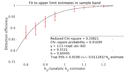
Figure 1: A demonstration of the upper limit validation technique for a sample band (101 Hz; October data). The x-axis is $h_{nom}$, $h_{0}$ divided by the ULE for this upper-limit band; the eight points represent detection efficiencies for eight sets of 125 software injections. These eight points are then fit to a sigmoid curve (in black); the 95% upper limit can then be read off from the point where the curve crosses 95% detection efficiency.

A small number of $0.1$-Hz bands had outliers so large that the semi-analytic method failed to converge to an estimate for $h_{0}$. Instrumental artifacts at these frequencies were identified using S6 run-averaged spectra and the respective 1-Hz bands were then rerun with the disturbed $0.1$-Hz subband excluded. The excluded bands are detailed in Table  4.

Affected 1-Hz Band	Vetoed 0.1-Hz subband	Artifact
180	180.0-180.1	Power mains harmonic
192	192.4-192.5	Hardware injection
217	217.5-217.6	Known instrumental artifact
234	234.0-234.1	Digital line (L1)
290	290.0-290.1	Digital line (L1)
370	370.1-370.2	L1 Output Mode Cleaner Line
393	393.1-393.2	Calibration line (H1)
396	396.7-396.8	Calibration Line (L1)
400	400.2-400.3	H1 Output Mode Cleaner Line
403	403.8-403.9	L1 Output Mode Cleaner Line
417	417.1-417.2	H1 Output Mode Cleaner Line
580	580.0-580.1	Digital line (L1)

Table 4: The twelve $0.1$-Hz bands with outliers too large for the semi-analytic method to converge to an estimate for $h_{0}$. These $0.1$-Hz subbands were excluded from upper limit analysis; the quoted upper limits (Figure  2) represent the remainder of their respective 1-Hz bands. The first column lists the affected 1-Hz band; the second column lists the respective vetoed 0.1-Hz subband; the third column lists the instrumental artifact identified using S6 run-averaged spectra.

III.2 Results

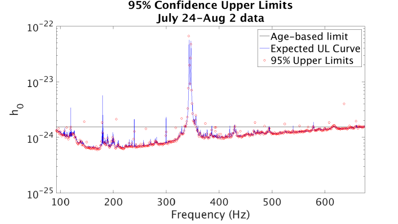
Figure 2: Upper limits at 95% confidence (red circles) compared to the upper limit estimate curve of the detector (blue curve) and the initial age-based limit on $h_{0}$ (black line). The upper limit estimate curve is based on Eq. (5) over the 9.2 days of coherence time, corrected for detector livetime and sky location and summed over detectors in inverse quadrature.

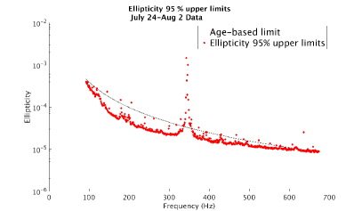
Figure 3: Upper limits at 95% confidence (red circles) compared to the initial age-based limit on fiducial ellipticity $\epsilon$ (black line).

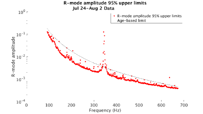
Figure 4: Upper limits at 95% confidence (red circles) compared to the initial age-based limit on $r$-mode amplitude $\alpha$ (black line).

Figure  2 shows the 95% confidence upper limits (ULs) over the full band for the July-August data set, which was the more sensitive of the two because of its much greater livetime (642 SFTs vs. 374 SFTs for the October data set). The blue curve represents the expected sensitivity of the search for this data set, computed from the power spectral density at each frequency; there is good agreement with the ULs. The black line represents the age-based limit derived when first considering the parameter space. Its intersection with the ULs at either end of the plot is a confirmation that we correctly estimated the frequency band to search over.

Figure  3 is a similar plot converting the upper limits on $h_{0}$ to upper limits on fiducial ellipticity $\epsilon$, using the formula Saulson1994

$$\epsilon=\frac{c^{4}}{4\pi^{2}G}\frac{d}{I_{zz}f^{2}}h_{0}.$$ (12)

The black curve represents the age-based limit on fiducial ellipticity, using the same assumptions (braking index $n=5$, age $\tau=300$ years) used in the parameter space calculations.

The amplitude $\alpha$ of $r$-mode oscillations in a neutron star is related to the gravitational wave strain amplitude $h_{0}$ by OwenRModes

$$\alpha=0.028\left(\frac{h_{0}}{10^{-24}}\right)\left(\frac{r}{1~{}\textup{kpc}}\right)\left(\frac{100~{}\textup{Hz}}{f}\right)^{3}.$$ (13)

Figure  4 uses this formula to convert the upper limits on $h_{0}$ to upper limits on the $r$-mode amplitude $\alpha$. The black curve represents the age-based limit on $\alpha$, under the same age assumptions used for $h_{0}$ and ellipticity, but with $n=7$, which characterizes $r$-mode emission. In all three plots, the age-based limit is beaten everywhere the upper limits lie below the black curve.

IV Discussion

This search has placed the first explicit upper limits on continuous gravitational wave strength from the nearby globular cluster NGC 6544 for spin-down ages as young as 300 years, and is the first directed CW search for any globular cluster. The most stringent upper limits on strain ($h_{0}^{\textup{UL}}$) obtained were $h_{0}^{\textup{UL}}=6.7\times 10^{-25}$ for the 173-174 Hz band in the October data set, and $h_{0}^{\textup{UL}}=6.0\times 10^{-25}$ for the 170-171 Hz band in the July-August data.

The best upper limit is comparable to the best upper limit of $7\times 10^{-25}$ at $150$ Hz obtained by the Cas A search S5CasA ; the recent search over nine supernova remnants, done without resampling, S6CasAFriends set upper limits as low as $3.7\times 10^{-25}$ for the supernova remnant G93.3+6.9, but used a coherence time of over 23 days (and a frequency band of only 264 Hz). The same analysis set a comparable 95% upper limit of $6.4\times 10^{-25}$ for the supernova remnant G1.9+0.3, as expected given its similar declination and the search’s similar coherence time (9.2 days for NGC 6544 vs. 9.1 days for G1.9+0.3). Note, however, that the G1.9+0.3 search was limited to a 146 Hz search band, compared to 583 Hz for NGC 6544. The search reported here was carried out at substantially less computational cost because of barycentric resampling, and could thus search over a much larger parameter space.

The best upper limit on fiducial ellipticity, established using the July-August data set, was $\epsilon=8.5\times 10^{-6}$, for the $1$-Hz band starting at $670$ Hz. This is comparable to the best upper limit ($4\times 10^{-5}$) obtained by the Cas A search Wette2009 ; the supernova remnant search S6CasAFriends set a comparable upper limit on fiducial ellipticity at $7.6\times 10^{-5}$ for the supernova remnant G1.9+0.3.

These ellipticities are within the range of maximum theoretical ellipticities predicted for stars with some exotic phases in the core OwenStrangeStars ; OwenJ-McD2013 , and the lowest of them is achievable for purely nucleonic stars with a sufficiently stiff equation of state and low mass OwenJ-McD2013 . Hence the search could have detected some exotic stars if they were supporting close to their maximum possible ellipticity; however, the lack of a detection cannot be used to infer constraints on the composition of any star, since the deformation could be much less than its maximum supportable value.

The first observing run of the Advanced LIGO detectors began in September 2015 Prospects and the sensitivity of the detectors is already three times or more better than that used in this search, with an order of magnitude improvement over S6 expected eventually AdvLIGO . The barycentric resampling algorithm first implemented in this search is being used extensively in CW searches in the advanced detector era; it has been integrated into the search codes for both coherent searches (like the supernova remnant search) IdrisyThesis and semi-coherent searches (Einstein@Home).

V Acknowledgments

The authors gratefully acknowledge the support of the United States National Science Foundation (NSF) for the construction and operation of the LIGO Laboratory and Advanced LIGO as well as the Science and Technology Facilities Council (STFC) of the United Kingdom, the Max-Planck-Society (MPS), and the State of Niedersachsen/Germany for support of the construction of Advanced LIGO and construction and operation of the GEO600 detector. Additional support for Advanced LIGO was provided by the Australian Research Council. The authors gratefully acknowledge the Italian Istituto Nazionale di Fisica Nucleare (INFN), the French Centre National de la Recherche Scientifique (CNRS) and the Foundation for Fundamental Research on Matter supported by the Netherlands Organisation for Scientific Research, for the construction and operation of the Virgo detector and the creation and support of the EGO consortium. The authors also gratefully acknowledge research support from these agencies as well as by the Council of Scientific and Industrial Research of India, Department of Science and Technology, India, Science & Engineering Research Board (SERB), India, Ministry of Human Resource Development, India, the Spanish Ministerio de Economía y Competitividad, the Conselleria d’Economia i Competitivitat and Conselleria d’Educació, Cultura i Universitats of the Govern de les Illes Balears, the National Science Centre of Poland, the European Commission, the Royal Society, the Scottish Funding Council, the Scottish Universities Physics Alliance, the Hungarian Scientific Research Fund (OTKA), the Lyon Institute of Origins (LIO), the National Research Foundation of Korea, Industry Canada and the Province of Ontario through the Ministry of Economic Development and Innovation, the Natural Science and Engineering Research Council Canada, Canadian Institute for Advanced Research, the Brazilian Ministry of Science, Technology, and Innovation, Fundação de Amparo à Pesquisa do Estado de São Paulo (FAPESP), Russian Foundation for Basic Research, the Leverhulme Trust, the Research Corporation, Ministry of Science and Technology (MOST), Taiwan and the Kavli Foundation. The authors gratefully acknowledge the support of the NSF, STFC, MPS, INFN, CNRS and the State of Niedersachsen/Germany for provision of computational resources.

This document has been assigned LIGO Laboratory document number LIGO-P1500225.

References

- (1) B. Abbott et al., Phys. Rev. D 69, 082004 (2004).
- (2) B. Abbott et al., Phys. Rev. Lett. 94, 181103 (2005).
- (3) B. Abbott et al., Phys. Rev. D 76, 042001 (2007).
- (4) B. Abbott et al., Ap. J. 683, L45 (2008).
- (5) J. Abadie et al., Ap. J. 737, 93 (2011), 1104.2712.
- (6) B. P. Abbott et al., Ap. J. 713, 671 (2010).
- (7) J. Aasi et al., Ap. J. 785, 119 (2014), 1309.4027.
- (8) B. Abbott et al., Phys. Rev. D 72, 102004 (2005).
- (9) B. Abbott et al., Phys. Rev. D 76, 082001 (2007).
- (10) B. Abbott et al., Phys. Rev. D 77, 022001 (2008).
- (11) B. Abbott et al., Phys. Rev. D 79, 022001 (2009).
- (12) B. P. Abbott et al., Phys. Rev. Lett. 102, 111102 (2009).
- (13) B. P. Abbott et al., Phys. Rev. D 80, 042003 (2009).
- (14) J. Abadie et al., Phys. Rev. D 85, 022001 (2012), 1110.0208.
- (15) J. Aasi et al., Phys. Rev. D 87, 042001 (2013), 1207.7176.
- (16) J. Aasi et al., Class. Quantum Grav. 31, 085014 (2014), 1311.2409.
- (17) J. Aasi et al., Class. Quantum Grav. 31, 165014 (2014), 1402.4974.
- (18) J. Aasi et al., Phys. Rev. D 90, 062010 (2014), 1405.7904.
- (19) B. Knispel and B. Allen, Phys .Rev. D 78, 044031 (2008), 0804.3075.
- (20) B. Abbott et al., Phys. Rev. D 76, 082003 (2007).
- (21) J. Abadie et al., Phys. Rev. Lett. 107, 261102 (2011), 1109.1809.
- (22) J. Abadie et al., Ap. J. 722, 1504 (2010).
- (23) K. Wette et al., Class. Quantum Grav. 25, 235011 (2008).
- (24) J. Aasi et al., Phys. Rev. D 88, 102002 (2013), 1309.6221.
- (25) J. Aasi et al., Ap. J. 813, 39 (2015), 1412.5942.
- (26) A. G. Lyne and F. Graham-Smith, Pulsar Astronomy, 3rd ed. (Cambridge University Press, 2006).
- (27) P. Jaranowski, A. Krolak, and B. F. Schutz, Phys. Rev. D 58, 063001 (1998), gr-qc/9804014.
- (28) C. Cutler and B. F. Schutz, Phys. Rev. D 72, 063006 (2005), gr-qc/0504011.
- (29) R. Prix and B. Krishnan, Class. Quantum Grav. 26, 204013 (2009), 0907.2569.
- (30) LAL/LALapps Software Suite, http://www.lsc-group.phys.uwm.edu/daswg/projects/lalsuite.html, Tag: CFSv2_singleIFO_DKOrder_for_real.
- (31) P. Astone, K. M. Borkowski, P. Jaranowski, M. Pietka, and A. Królak, Phys. Rev. D 82, 022005 (2010), 1003.0844.
- (32) P. Patel, X. Siemens, R. Dupuis, and J. Betzwieser, Phys. Rev. D 81, 084032 (2010), 0912.4255.
- (33) P. Patel, Search for Gravitational Waves from a nearby neutron Star using barycentric resampling, PhD thesis, California Institute of Technology, 2010.
- (34) Z.-X. Wang, D. Chakrabarty, and D. L. Kaplan, Nature 440, 772 (2006), astro-ph/0604076.
- (35) A. Wolszczan and D. A. Frail, Nature 355, 145 (1992).
- (36) S. E. Thorsett, Z. Arzoumanian, and J. H. Taylor, Ap. J. Lett. 412, L33 (1993).
- (37) S. Sigurdsson, H. B. Richer, B. M. Hansen, I. H. Stairs, and S. E. Thorsett, Science 301, 193 (2003), astro-ph/0307339.
- (38) S. Sigurdsson, Ap. J. Lett. 399, L95 (1992).
- (39) M. Vigelius and A. Melatos, Mon. Not. Roy. Astron. Soc. 395, 1985 (2009), 0902.4484.
- (40) B. Haskell et al., Mon. Not. Roy. Astron. Soc. 450, 2393 (2015), 1501.06039.
- (41) F. Verbunt and P. Hut, The Globular Cluster Population of X-Ray Binaries, in The Origin and Evolution of Neutron Stars, edited by D. J. Helfand and J.-H. Huang, , IAU Symposium Vol. 125, p. 187, 1987.
- (42) W. E. Harris, Astron. J. 112, 1487 (1996).
- (43) W. E. Harris, ArXiv e-prints (2010), 1012.3224.
- (44) K. Wette, Phys. Rev. D 85, 042003 (2012), 1111.5650.
- (45) D. M. Whitbeck, Observational consequences of gravitational wave emission from spinning compact sources, PhD thesis, The Pennsylvania State University, 2006.
- (46) R. Prix, Phys. Rev. D 75, 023004 (2007), gr-qc/0606088.
- (47) B. J. Owen, Phys. Rev. D 53, 6749 (1996), gr-qc/9511032.
- (48) P. R. Brady, T. Creighton, C. Cutler, and B. F. Schutz, Phys. Rev. D 57, 2101 (1998), gr-qc/9702050.
- (49) D. Heggie and P. Hut, The Gravitational Million-Body Problem: A Multidisciplinary Approach to Star Cluster Dynamics (Cambridge University Press, 2003).
- (50) D. Keitel, R. Prix, M. A. Papa, P. Leaci, and M. Siddiqi, Phys. Rev. D 89, 064023 (2014), 1311.5738.
- (51) K. Wette, Gravitational waves from accreting neutron stars and Cassiopeia A, PhD thesis, Australian National University, 2009.
- (52) P. Saulson, Fundamentals of Interferometric Gravitational Wave Detectors (World Scientific Publishing Company, Incorporated, 1994).
- (53) B. J. Owen, Phys. Rev. D 82, 104002 (2010), 1006.1994.
- (54) B. J. Owen, Phys. Rev. Lett. 95, 211101 (2005), astro-ph/0503399.
- (55) N. K. Johnson-McDaniel and B. J. Owen, Phys. Rev. D 88, 044004 (2013), 1208.5227.
- (56) B. P. Abbott et al., Living Rev. Relat. 19 (2016), 1304.0670.
- (57) LIGO Scientific Collaboration et al., Class. Quantum Grav. 32, 074001 (2015), 1411.4547.
- (58) A. Idrisy, Searching for Gravitational Waves from Neutron Stars, PhD thesis, The Pennsylvania State University, 2015.