Large Scale GPU Accelerated PPMLR-MHD Simulations for Space Weather Forecast

Abstract

PPMLR-MHD is a new magnetohydrodynamics (MHD) model used to simulate the interactions of the solar wind with the magnetosphere, which has been proved to be the key element of the space weather cause-and-effect chain process from the Sun to Earth. Compared to existing MHD methods, PPMLR-MHD achieves the advantage of high order spatial accuracy and low numerical dissipation. However, the accuracy comes at a cost. On one hand, this method requires more intensive computation. On the other hand, more boundary data is subject to be transferred during the process of simulation. In this work, we present a parallel hybrid solution of the PPMLR-MHD model implemented using the computing capabilities of both CPUs and GPUs. We demonstrate that our optimized implementation alleviates the data transfer overhead by using GPU Direct technology and can scale up to 151 processes and achieve significant performance gains by distributing the workload among the CPUs and GPUs on Titan at Oak Ridge National Laboratory. The performance results show that our implementation is fast enough to carry out highly accurate MHD simulations in real time.

I Introduction

The magnetosphere, which is the outermost of the geospace, is formed when the solar wind interacts with the Earth’s internal magnetic field [1]. Understanding the formation and development of the magnetosphere is crucial because it is the key element of the space weather cause-and-effect chain process from the Sun to the Earth. Similar to the weather on Earth, space weather is about the time varying conditions taking place in the space from the solar atmosphere to the geospace. It is driven by the solar wind which carries solar energy and comes through interplanetary space from the near surface of the Sun and the Sun’s atmosphere. Due to the effect of the Earth’s magnetic field, the magnetosphere forms a shape similar to a bullet, where the sunny side is roughly like a hemisphere with a radius of 15$R_{E}$(Earth radii), while the nightside forms a cylinder shape with a radius of 20-25$R_{E}$. The tail region stretches well beyond 200$R_{E}$ while its exact length is not well known. It is known that the geospace, including the magnetosphere and ionosphere, has the nature of nonlinearity, multiple-component, and time-dependence, which together pose a big challenge to investigate it using only traditional analytical approaches. Therefore, numerical models have been developed to explore the properties of the solar wind-magnetosphere-ionosphere coupling. It has been demonstrated that this kind of study is a natural match for MHD numerical simulations[1].

Over the years, different global MHD models have been developed to study the cause-and-effect of the space weather: 1) Lax-Wendroff model [2], 2) FV-TVD model [3], 3) OpenGGCM model [4], 4) GUMICS-3 model [5], 5) LFM model [6], 6) BATS-R-US model [7], and 7) PPMLR-MHD model [1]. The PPMLR-MHD model is a new global MHD model, which achieves high order spatial accuracy and low numerical dissipation compared to other existing models. By applying the piecewise parabolic method, the PPMLR-MHD algorithm has an accuracy of a third order in space, which enables the numerical model to present physical solutions even using relatively larger grid spacing. However, the parabolic interpolation is more complex than other interpolations, i.e. the linear interpolation, and therefore the computation amount will cost more time. Besides, this interpolation advancement also requires more communication data transfer. These problem together pose big challenge to develop a highly efficient fast implementation.

The development of the General-Purpose GPU technology in recent years has made big progress in the field of high performance computing. Due to the massive parallelism nature of GPUs, researchers are now able to solve large scale problems at a much faster speed while using less power. As of now NVIDIA has released its 4th-gen CUDA devices capable of running thousands of parallel threads simultaneously. However, GPU programming is very different from that of CPU as it has a very specific architecture, one needs to carefully design the architecture of the software to maximize the performance. Meanwhile, since GPU has its own dedicated memory, concerns also need to be addressed in minimizing the overhead of data transfer.

In this work, we present a GPU implementation of the PPMLR-MHD model. Due to the computation and data transfer intensive nature of this model, special attention has been paid to alleviate the overhead during simulation. We discuss the parallel problem partition, followed by the adaptation design scheme for taking advantage of the latest NVIDIA GPUs. We also demonstrate the techniques adopted to alleviate data transfer overhead using GPU direct techniques. We scale our implementation to hundreds of processes and solve the MHD simulation problem in a very efficient manner to meet the real time requirements for space weather forecast.

II The PPMLR-MHD Method

The global numerical model for Earth’s space environment, especially for the magnetosphere is based on the magnetohydrodynamic (MHD) description of plasma. The conservational form of the 3-Dimensional MHD equations is listed as follows:

$$\frac{\partial\rho}{\partial t} +\nabla\cdot(\rho\mathbb{v})=0$$

$$\frac{\partial(\rho\mathbb{v})}{\partial t} +\nabla\cdot(\rho\mathbb{v}\mathbb{v}+p^{\ast}\mathbb{I}-\frac{1}{\mu_{0}}\mathbb{B}^{{}^{\prime}}\mathbb{B}^{{}^{\prime}})=(\nabla\times\mathbb{B}^{{}^{\prime}})\times\mathbb{B_{d}}$$

$$\frac{\partial\mathbb{B}^{{}^{\prime}}}{\partial t} +\nabla\cdot(\mathbb{v}\mathbb{B}^{{}^{\prime}}-\mathbb{B}^{{}^{\prime}}\mathbb{v})=\nabla\times(\mathbb{v}\times\mathbb{B_{d}})-\mathbb{v}\nabla\cdot\mathbb{B}^{{}^{\prime}}$$

$$\begin{split}\frac{\partial E}{\partial t}&+\nabla\cdot[(E+p^{\ast})\mathbb{v}-\frac{1}{\mu_{0}}(\mathbb{v}\cdot\mathbb{B}^{{}^{\prime}})\mathbb{B}^{{}^{\prime}}]=\\ &\;\quad\mathbb{v}\cdot[(\nabla\times\mathbb{B}^{{}^{\prime}})\times\mathbb{B_{d}}]+\mathbb{B}^{{}^{\prime}}\cdot[\nabla\times(\mathbb{v}\times\mathbb{B_{d}})]\end{split}$$

where

$$\mathbb{B}^{{}^{\prime}} =\mathbb{B}-\mathbb{B_{d}},p^{\ast}=p+\frac{B^{{}^{\prime}2}}{2\mu_{0}},$$

$$E =\frac{p}{\gamma-1}+\frac{1}{2}\rho v^{2}+\frac{B^{{}^{\prime}2}}{2\mu_{0}},$$

$\rho$ is the density, $p$ is the plasma pressure, $\mathbb{v}$ is the flow velocity, $\mathbb{B},\mathbb{B_{d}},\mathbb{B^{{}^{\prime}}}$ are the magnetic field, the Earth’s dipole field, and the difference between the two fields respectively, $\mu_{0}=4\pi\times 10^{-7}\text{H}\cdot\text{m}^{-1}$ is the permeability of vacuum and $\gamma=5/3$ is the adiabatic index. In order to improve the accuracy in the calculation of the magnetic field, $\mathbb{B^{{}^{\prime}}}$ is evaluated instead of $\mathbb{B}$ during the simulations, for the Earth’s dipole field could be very large when closer to Earth. But it is noted that $\mathbb{B^{{}^{\prime}}}$ does not have to be small compared with $\mathbb{B_{d}}$.

A so-called piecewise parabolic method with a Lagrangian remap (PPMLR)-MHD algorithm, developed by Hu etc. [1], is applied to solve these equations. It is an extension of the Lagrangian version of the Piecewise Parabolic Method (PPMLR) developed by Collela & Woodward [8] to MHD. In this PPMLR-MHD algorithm, all variables ($\rho$, $\mathbb{v}$, $\mathbb{B^{{}^{\prime}}}$ and $p$) are defined at the zone centers as volume averages, and their spatial distributions can be obtained by a parabolic interpolation which is piecewise continuous in each zone. When a characteristic method is used to calculate the local values of the variables at the zone edges, they are updated first in the Lagrangian coordinates to the next time step, and then the results are remapped onto the fixed Eulerian grids by solving the corresponding advection equations.

For the closure of the field-aligned current, an ionosphere shell, setting at r = 1.017$R_{E}$ (110 km altitude) is integrated in the simulation model under the electrostatic assumptions, which is connected with the magnetospheric inner boundary, setting at r = 3$R_{E}$ by dipole field lines between them. An electrostatic potential equation is solved in the ionosphere, and the solved potential is mapped to the magnetospheric inner boundary as a boundary condition for magnetospheric flows.

More numerical details of the simulation model can be found in [1], and a number of studies of the solar wind-magnetosphere-ionosphere interactions have been successfully carried out based on this model, and have been reviewed in [9].

III The Hybrid Implementation

III-A Task Partitioning

The numerical domain of the PPMLR-MHD model is over a stretched Cartesian coordinate which takes the Earth as the origin and lets the x, y, and z axes point to the Sun, dusk, and the northward directions, respectively. The size of this domain extends from 30 $R_{E}$ to -100 $R_{E}$ along the Sun-Earth line and from -100 $R_{E}$ to 100 $R_{E}$ in y and z directions. It is discretized into 156 $\times$ 150 $\times$ 150 grid points: the grid is rectangular and nonuniform with the highest spatial resolution of 0.4 $R_{E}$ near Earth. To accommodate the large simulation volume and long simulation time, we parallelize the model to be scalable from several to hundreds of processes , and partion the domain in all three directions. For the purpose of load balance, each subdomain usually contains the same number of grid points. Since the subdomain that contains the Earth must stay in a single numerical grid, the number of processes in the y and z direction must be odd (1, 3, 5, etc.). In addition, one more process is required to solve the ionospheric potential equation. It is worthy to point out that the 3-Dimensional MHD equations on every grid in each subdomain is divided into three 1-Dimensional equations, which are independent in the other two directions when solving these one dimensional equations. As 156 is divisible by 3, 4 and 6, we employ the process configuration of 3 $\times$ 1 $\times$ 1, 3 $\times$ 3 $\times$ 3, 4 $\times$ 3 $\times$ 3, 6 $\times$ 3 $\times$ 3, 4 $\times$ 5 $\times$ 5, 6 $\times$ 5 $\times$ 5, plus one more process, the final number of processes are 4, 28, 37, 55, 101, 151, respectively.

III-B Optimisation Analysis and Design for GPU

GPU is different in hardware architecture compared to CPU in that it focuses more on the part of parallel computation in large scale. To maximize the computational power of the GPU, attentions have to be paid at the design phase of the GPU code implementation. This section first describes the general optimisation methods in GPU programming and then discusses the high performance design considerations adopted in our PPMLR-MHD implementation. In this work we employ NVIDIA’s CUDA as our GPU programming tool, therefore the optimisation terminologies demonstrated are limited to CUDA.

III-B1 Overview of Optimisation Methods

In essence, GPU is a massively parallel device which is capable of running tens of thousands of tasks simultaneously. Similar to CPU, the basic GPU execution unit is termed as GPU thread. To achieve high efficiency on GPU, it is required that the GPU threads launched are well past the number of executable threads (tens of thousands) so that hanging and ready threads can be switched back and forth dynamically to hide load/store instruction latency. The general optimisation methods include (but not limited): a) increasing the occupancy ([10, 11]), which is defined as the ratio between the active executing threads and the maximal executable threads on GPU streaming multiprocessor (SMX), b) employing coalesced memory access pattern (adjacent threads access adjacent memory addresses in short) for global memory read/write, c) shared memory tuning for reusable data access, d) atomic optimisation [12] for superposition that involves small scale memory conflict (no greater than 16 threads per memory address), e) warp shuffle optimisation for reduction, f) streaming for increasing multiprocess GPU resources utilization.

III-B2 High Efficiency Design

Our goal is to achieve high efficiency, high performance while maintaining high accuracy. In an effort to achieve this goal, we concentrate our effort on the following four aspects in designing the implementation: a) Adopt non-uniform spacing strategy in choosing numerical grids to reduce unnecessary computation. In our PPMLR-MHD model, a uniform mesh is laid out in the near-Earth domain within 10$R_{E}$, and the grid spacing outside increases according to a geometrical series of common ratio of 1.05 along each axis. b) Reorganize the data so that it’s GPU memory efficient. The memory-bound nature of the PPMLR-MHD method makes it very important to efficiently access the data as the whole simulation process consists of tens of thousands of time steps. In each step, the boundary input is obtained from neighbouring MPI processes and employed only once to solve the equations described in section II. As a result, GPU’s shared memory is no longer needed for optimisation which makes global memory access with coalesced pattern very important. In addition, each solving process contains only basic arithmetic, no reduction or memory conflict is involved, therefore warp-shuffle and atomic optimisation are not helpful in our case. c) Employ streaming strategy to make the most of GPU resources. As kernels in different GPU streams can make use of the GPU parallelly, we make every grid execute in a specific stream. d) Make use of CUDA-aware MPI to efficiently transfer data between MPI ranks. In traditional MPI programming, the data computed on GPU has to be transferred back into CPU’s host memory and then sent to responding MPI processes via MPI message. This is a big overhead as unnecessary data transfer is totally a waste of time. In our implementation, each grid needs to obtain boundary data from neighbouring processes in each step and there are more than thousands of steps performed, which makes the data transfer even more severe. To address this problem, we take advantage of the CUDA-aware MPI. Besides the capability of transferring data pointers pointed to host memory, the CUDA-aware MPI also takes care of GPU’s device memory, which significantly reduces the unnecessary data movement by directly move data between GPUs by taking advantage of network adapter’s RDMA capability. Figure 1 illustrates the data movement difference between traditional MPI and CUDA-aware MPI. The long solid arrow in the upper part of the figure shows the data flow of the CUDA-aware MPI, the rest of the arrows shows the data flow of the traditional MPI.

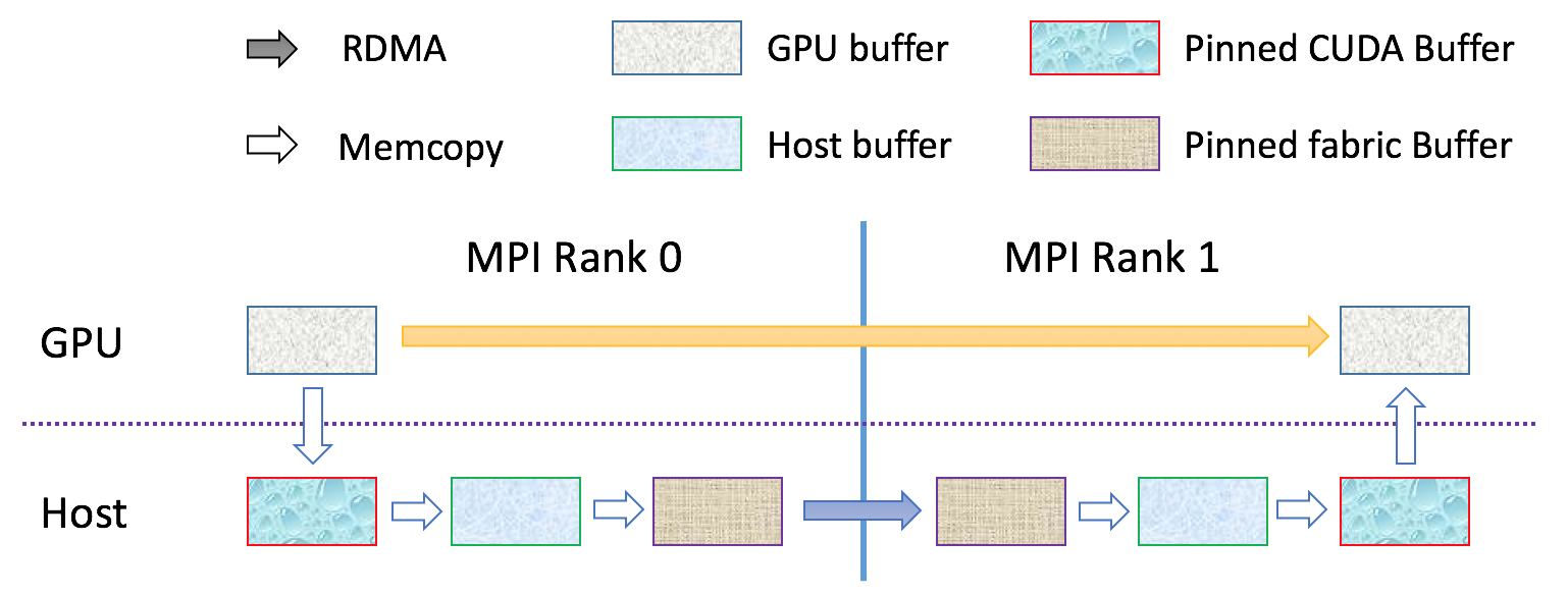
Figure 1: Comparison between traditional MPI and CUDA-aware MPI. The CUDA-aware MPI directly transfers data via RDMA while avoiding unnecessary data movement compared to the traditional MPI.

IV Performance and Scalability Study

This section discusses the performance and scalability of the GPU PPMLR-MHD implementation. To begin with, we study the scalability of the simulation, which gives a general performance picture of our MHD method. We then discuss more specific topics including single process performance and the transfer time of each process in different execution configurations.

IV-A Testing environment

We test our implementation on the Titan Supercomputer at the Oak Ridge National Laboraty (ORNL), the hardware and software configuration of each computing node is shown in Table I, each node is equipped with two 10-core CPUs as well as one NVIDIA GPU.

TABLE I: Compute Node Configuration

CPU	AMD Opteron™ 6274 (Interlagos)
GPU	NVIDIA Tesla K20x
Host Max Memory Bandwidth	51.2 GB/s
GPU Max Memory Bandwidth	250 GB/s
Network	40 Gb/s Infiniband
Memory	32 GB
OS	Cray Node Linux (CNL)
CUDA Version	7.5

In the case of the PPMLR-MHD simulation, the input scale depends on the resolution of the numerical grids, which is predetermined in the design phase of this method. In other words, the input scale is fixed. Therefore, we focus on the strong scalability of the PPMLR-MHD simulation. We test our implementation with 4, 28, 37, 55, 101, 151 processes, respectively, and then look into detailed performance results on both computation and data transfer. The reason we choose these irregular numbers is that the PPMLR task partition scheme has its own constraint: the number of ranks in the y and z direction must be odd and the same as each other, plus one more MPI rank is used for calculating the boundary update information. To perform the simulation, we start with a somewhat arbitrarily prescribed initial state. In the domain of x $\leqslant$ 15$R_{E}$, B’ (defined in section II) is produced by the image of Earth’s dipole located at (x, y, z) = (30, 0, 0)$R_{E}$, and the initial distribution of plasma density and temperature is spherically symmetric. Finally, on the right of x = 15$R_{E}$, a uniform solar wind and a uniform interplanetary magnetic field (IMF) are assumed. The simulation will continue until a steady-state magnetosphere is reached.

IV-B Scalability and Accuracy study

The accuracy and utility of space weather forecasts depend heavily on a thorough knowledge of the Sun-Earth system. The PPMLR-MHD model is designed to have high order spatial accuracy and low numerical dissipation. To further improve the accuracy in the calculation of the magnetic field, we have subtracted the Earth’s dipole field from the total, and only the deviation field B’ is evaluated during the calculations. For the simulation, a given numerical accuracy can be achieved by using a corresponding numerical grids partition. In this work, we choose a relatively middle numerical grids ($156\times 150\times 150$) which is most frequently used in our daily working environment.

Since the overall problem for a given accuracy can be considered as fixed for a given accuracy, we discuss the strong scalability of the problem and omit the study of weak scalability. The strong scalability of the PPMLR-MHD method is determined by the size of the numerical grids. In our experiment configuration, the numerical grids is chosen to be $156\times 150\times 150$. To facilitate implementation, we add extra constraint to our task partition strategy: the number of MPI ranks in the y and z axis must be the same and they are required to be odd numbers. PPMLR-MHD employs an iterative method to solve the MHD equations, in each iteration of the simulation, each grid (computed by a single MPI rank) needs to exchange its boundary data from all of its neighbours, the total amount of data required to be exchanged (TDE) is proportional to the partition choice applied. The amount of data exchanged in z direction can be represented as $c\times n_{x}\times n_{y}\times(n_{z}-1)$ where c represents a certain constants and $n_{x},n_{y},n_{z}$ is the number of MPI ranks in the x, y, z dimensions, respectively, x and y direction can be calculated in the same way, there fore, TDE can be calculated as:

$$\begin{split}TDE&\propto n_{x}\times n_{y}\times(n_{z}-1)\\ &+n_{x}\times(n_{y}-1)\times n_{z}\\ &+(n_{x}-1)\times n_{y}\times n_{z}\end{split}$$ (1)

From equation 1, the total number of MPI ranks has positive relation to the total amount of exchanged data, involving more GPUs also brings more data transfer overhead. Besides, GPU requires problem to be big enough in order to take advantage of its massive parallel power. A compromise has to be made between the computation resources and the data exchange overhead. To demonstrate, we simulate our implementation for 100 iterations since the total amount of execution time required for several execution configuration is too long. Figure 2 shows the simulation results.

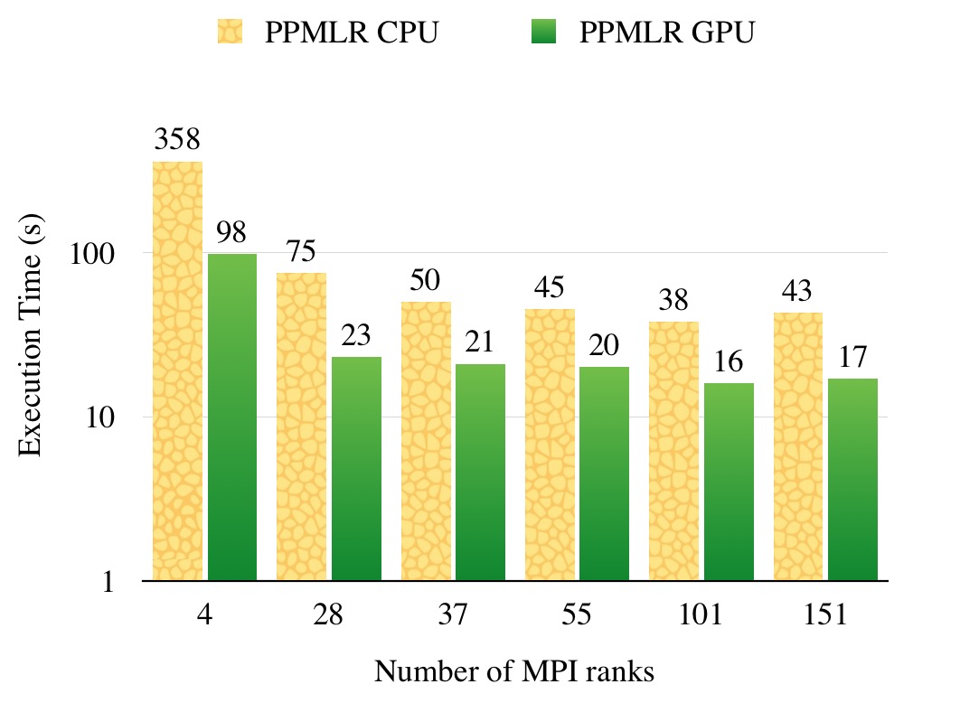
Figure 2: Execution time of simulations for 100 iterations in different scale configuration.

As illustrated in the figure, in every chosen execution configuration, our GPU PPMLR-MHD implementation outperforms the CPU counterpart (2.5 to 3.5 times faster). The best performance comes from the execution configuration of 101 MPI ranks, this result meets our expectation, because more processes bring not only more computational resources but also more data exchange overhead, the execution configuration of 101 processes is the balance point between these two performance related factors.

IV-C GPU performance study

The computing capability of GPU plays a key role for us to achieve real time simulation. This section studies the performance contribution of GPU. To begin with, we compare our GPU implementation with a CPU counterpart which is highly optimised for spatial-temporal locality memory access. To accurately measure the computation performance, we randomly choose several single steps and record the computation time from each MPI rank, we then average the sum of all records and use the final result to perform comparison. Since the computing workload for each step is predetermined and thus fixed, each step is supposed to take approximately the same amount of time. Our results give a direct comparions of the code performance on GPU and CPU.

Although parallelization is well considered in the design process of the PPMLR-MHD implementation, the memory-intensive nature of the algorithm makes it more memory bandwidth limited when considering the expected performance. In theory, the PPMLR-MHD GPU implementation’s maximum achievable speedup (MAS) over the CPU counterpart can be expressed as:

$$MAS=\frac{GPU\ Memory\ Bandwidth}{Host\ Memory\ Bandwidth}$$

From the hardware configuration listed in Table I, the maximum expected speedup should be MAS = 250 GB/s / 52 GB/s $\approx$ 4.88 in our testing environment. Figure 3 illustrates the execution time of a single step in different scale configurations.

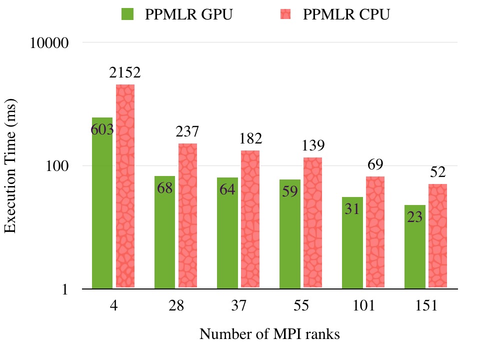
Figure 3: Average execution time of each step in different scale configurations. The number in the x axis stands for the number of processes used in launching MPI executables.

As can be seen in the figure, the employment of GPU has significantly improves the performance of the PPMLR simulation. The GPU version has achieved up to 3.57x speedups (compared to the CPU counterpart) in the configuration of 4 MPI ranks. This result is very close to the MAS theoretical peak of 4.88 (73.2 % of the GPU bandwidth has been employed). As the number of MPI ranks increases, the effect of GPU acceleration is less significant, this is due to the fact that the increasing of parallel processes results in the decreasing of the amount of workload in each MPI rank. When the workload is below a certain amount, GPU is underutilize thus unable to achieve peak performance.

IV-D Data transfer time study

Heterogeneous computing devices such as GPU have their own dedicated memory. Data that are used as input to execute are required to reside on GPU’s device memory, as the host memory is not accessible from GPU streaming multiprocessors. For many traditional MPI-based scientific applications such as PPMLR-MHD, this causes a major problem in using multiple GPUs since the computed results must be transferred back and forth from GPU memory to CPU’s host memory in order to update boundary data on the numerical grids. Arrows in the lower part of Figure 1 demonstrates the data flow from one GPU to another using traditional MPI. As can be seen, except for the necessary RDMA operation, there are 6 more memory copy operations involved in a single data transfer between two MPI ranks. Obviously, the redundant 6 memory copy operations per MPI rank pair causes a bandwidth overhead that is non-ignorable in achieving high performance.

To reduce the data transfer overhead, we employ the CUDA-aware MPI. Through this technology, the GPU’s device memory can be directly sent to/received from the MPI api, combined with Remote Direct Memory Access (RDMA) technology, buffers can be directly sent from GPU memory to a network adapter without staging through host memory, as shown in the upper part of Figure 1. Therefore, compared to a CPU counterpart using traditional MPI implementation, our PPMLR-MHD GPU version is supposed to take approximately the same amount of time in transferring data. We predict that

$$CPU\ data\ transfer\ time\approx GPU\ data\ transfer\ time$$

To check our prediction, we randomly choose a single simulation step from both PPMLR-MHD GPU implementation and the CPU counterpart, we record the total amount of time taken for sending as well as receiving data for all MPI ranks involved, we then average them and use the result as the comparison input. Since the amount of data being transferred is exactly the same for every single step, the choice of the experiment design is supposed to demonstrate the accurate data transfer overhead difference between the CPU and GPU implementation.

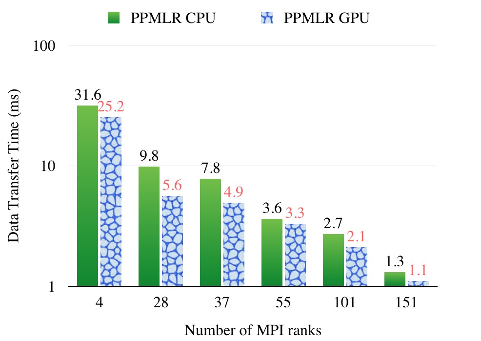
Figure 4: Average data transfer time of each step in different scale configurations. The number in the x axis represents the number of processes used in launching MPI executables.

Figure 4 shows the comparison of the data transfer time of the PPMLR GPU implementation versus that of the CPU counterpart in different execution configurations. As presented in the figure, the PPMLR GPU implementation takes slightly less time in transferring data compared to the CPU counterpart. We attribute this result to the employment of the CUDA-aware MPI as well as GPU’s high speed memory bus. CUDA-aware MPI helps our implementation to take advantage of the RDMA in transferring data among MPI ranks, as the CPU version also uses this technology, we expect the two implementations spend approximately the same amount of time in transferring data. The reason PPMLR GPU takes less time is due to the fact that GPU has higher speed bus, thus data from GPU’s device memory reaches network adaptor quicker than that from host memory.

V Conclusion

In this work, we present a GPU accelerated implementation of the PPMLR-MHD model for space weather forecast. We significantly improve the code performance by taking advantage of the GPU technology as well as CUDA-aware MPI. By making careful choices in the design phase of the implementation, we are able to make the most of GPU’s powerful compute capability and achieve near peak performance. The final implementation is scaled to up to 151 processes and the real time performance requirement is met.

References

- [1] Y. Hu, X. Guo, and C. Wang, “On the ionospheric and reconnection potentials of the earth: Results from global mhd simulations,” Journal of Geophysical Research: Space Physics, vol. 112, no. A7, 2007.
- [2] T. Ogino, R. J. Walker, and M. Ashour-Abdalla, “A global magnetohydrodynamic simulation of the magnetosheath and magnetosphere when the interplanetary magnetic field is northward,” Plasma Science, IEEE Transactions on, vol. 20, no. 6, pp. 817–828, 1992.
- [3] T. Tanaka, “Finite volume tvd scheme on an unstructured grid system for three-dimensional mhd simulation of inhomogeneous systems including strong background potential fields,” Journal of Computational Physics, vol. 111, no. 2, pp. 381–389, 1994.
- [4] J. Raeder, R. Walker, and M. Ashour-Abdalla, “The structure of the distant geomagnetic tail during long periods of northward imf,” Geophysical research letters, vol. 22, no. 4, pp. 349–352, 1995.
- [5] P. Janhunen, “Gumics-3 a global ionosphere-magnetosphere coupling simulation with high ionospheric resolution,” in Environment Modeling for Space-Based Applications, vol. 392, 1996, p. 233.
- [6] J. Lyon, J. Fedder, and C. Mobarry, “The lyon–fedder–mobarry (lfm) global mhd magnetospheric simulation code,” Journal of Atmospheric and Solar-Terrestrial Physics, vol. 66, no. 15, pp. 1333–1350, 2004.
- [7] K. G. Powell, P. L. Roe, T. J. Linde, T. I. Gombosi, and D. L. De Zeeuw, “A solution-adaptive upwind scheme for ideal magnetohydrodynamics,” Journal of Computational Physics, vol. 154, no. 2, pp. 284–309, 1999.
- [8] P. Colella and P. R. Woodward, “The piecewise parabolic method (ppm) for gas-dynamical simulations,” Journal of computational physics, vol. 54, no. 1, pp. 174–201, 1984.
- [9] C. Wang, X. Guo, Z. Peng, B. Tang, T. Sun, W. Li, and Y. Hu, “Magnetohydrodynamics (mhd) numerical simulations on the interaction of the solar wind with the magnetosphere: A review,” Science China Earth Sciences, vol. 56, no. 7, pp. 1141–1157, 2013.
- [10] C. Nvidia, “Programming guide,” 2008.
- [11] C. CUDA, “Best practice guide, 2013,” 2013.
- [12] X. Guo, X. Liu, P. Xu, Z. Du, and E. Chow, “Efficient particle-mesh spreading on gpus,” Procedia Computer Science, vol. 51, pp. 120–129, 2015.