Sapo: Reachability Computation and Parameter Synthesis of Polynomial Dynamical Systems

Abstract

Sapo is a C++ tool for the formal analysis of polynomial dynamical systems. Its main features are: 1) Reachability computation, i.e., the calculation of the set of states reachable from a set of initial conditions, and 2) Parameter synthesis, i.e., the refinement of a set of parameters so that the system satisfies a given specification. Sapo can represent reachable sets as unions of boxes, parallelotopes, or parallelotope bundles (symbolic representation of polytopes). Sets of parameters are represented with polytopes while specifications are formalized as Signal Temporal Logic (STL) formulas.

I Introduction

Formal verification involves the strict and exhaustive study of systems using mathematically based techniques. The development and application of formal methods is motivated by the fact that the formal study of a model implies the reliability and robustness of the abstracted system.

Two important problems emerging from the formal analysis of dynamical systems are the reachability computation and the parameter synthesis problems. In the first case, for a given set of initial conditions, it is asked to compute the set of states reachable by the dynamical system. In the second case, an initial set of conditions together with a set of parameters and a specification are provided, and it is asked to refine the set of parameters in such a way that the system satisfies the specification. These two problems often recur in formal analysis. For instance, the reachability computation can be used to determine whether a systems reaches some undesired states or remains within a particular subset of the state space, while synthesis of parameters can be used to design dynamical systems and tune their parameters so that to fit experimental observations or satisfy requirements.

Despite the numerous tools available for the analysis of linear dynamical systems (i.e., systems whose dynamics are linear functions), not many tools for the study of nonlinear systems are available. The main difficulties arising from nonlinearity concern the transformation of sets with respect to nonlinear functions. This operation, in general, does not preserve nice properties of the sets (e.g., convexity), and thus approximation techniques, that often suffer in terms of scalability, are necessary.

In this work we present Sapo [1], a C++ tool that targets discrete-time polynomial dynamical systems (possibly equipped with parameters) and that deals with both the reachability computation and parameter synthesis problems. Sapo can be used either to generate flowpipes that over-approximate reachable sets over bounded time horizons, or to refine sets of parameters in such a way that the system satisfies a Signal Temporal Logic (STL) [17] specification. The tool allows the construction of flowpipes using boxes (i.e., hyperrectangles), parallelotopes (i.e., $\displaystyle n$-dimensional parallelograms), or parallelotope bundles (i.e., sets of parallelotopes whose intersections symbolically represent polytopes), and the refinement of parameter sets represented by polytopes. Sapo’s underlying algorithms exploit some properties of Bernstein coefficients of polynomials. Intuitively, the Bernstein coefficients can be used to bound a polynomial over the unit box domain (i.e., $\displaystyle[0,1]^{n}$). The core idea on which Sapo relies is the transformation of unit boxes into generic sets. With this trick, Sapo exploits Bernstein coefficients to maximize polynomials and determine sets that over-approximate the trajectories of the system. A similar approach is also used to reduce the parameter synthesis problem into linear programs, where the linear systems, constructed through parameterized Bernstein coefficients, represent sets of valid parameters. The algorithms implemented in Sapo are based on the theoretical results exposed in [8, 11, 6, 7, 12, 10].

II Reachability and Parameter Synthesis

Sapo deals with discrete-time parametric polynomial dynamical systems described by difference equations of the form:

$$~{}x_{k+1}=f(x_{k},p)$$ (1)

where $\displaystyle f:\mathbb{R}^{n}\times\mathbb{R}^{m}\to\mathbb{R}^{n}$ is a polynomial linear in $\displaystyle p$, $\displaystyle x_{k}\in\mathbb{R}^{n}$ is the state of the system at time $\displaystyle k\in\mathbb{N}$, and $\displaystyle p\in\mathbb{R}^{m}$ are the parameters. Given an initial condition $\displaystyle x_{0}\in\mathbb{R}^{n}$ and parameters $\displaystyle p\in\mathbb{R}^{m}$, the trajectory $\displaystyle x_{0},x_{1},x_{2},\dots$ describing the evolution the system, can be obtained by iterating the function (1). The problems addressed by Sapo are:

• Reachability computation: Given a set of initial conditions $\displaystyle X_{0}\subset\mathbb{R}^{n}$, a set of parameters $\displaystyle P\subset\mathbb{R}^{m}$, and a time instant $\displaystyle T\in\mathbb{N}$, determine a sequence of tight sets $\displaystyle X_{0},X_{1},X_{2},\dots X_{T}$, called flowpipe, such that all the trajectories of length $\displaystyle T$ with initial conditions in $\displaystyle X_{0}$ and parameters in $\displaystyle P$ are included in the constructed flowpipe;

• Parameter synthesis: Given a set of initial conditions $\displaystyle X_{0}\subset\mathbb{R}^{n}$, a set of parameters $\displaystyle P\subset\mathbb{R}^{m}$, and a specification $\displaystyle\varphi$, determine the largest set $\displaystyle P_{\varphi}\subseteq P$ such that all the trajectories with initial conditions in $\displaystyle X_{0}$ and parameters in $\displaystyle P_{\varphi}$ satisfy $\displaystyle\varphi$.

III Main Features

III-A Bernstein Coefficients

At the core of Sapo for both reachability computation and parameter synthesis there are Bernstein coefficients of polynomials. Intuitively, Bernstein coefficients can be used to represent a polynomial in Bernstein form, i.e., as the linear combination of Bernstein basis and coefficients. Given a polynomial $\displaystyle\pi:\mathbb{R}^{n}\to\mathbb{R}$:

$$\pi(x)=\sum_{i\in I^{\pi}}a_{i}x^{i}$$ (2)

where $\displaystyle i=(i_{1},\dots,i_{n})\in\mathbb{N}^{n}$ is a multi-index, $\displaystyle x^{i}=x_{1}^{i_{1}}\dots x_{n}^{i_{n}}$ is a monomial, $\displaystyle a_{i}\in\mathbb{R}$ is a coefficient, and $\displaystyle I^{\pi}\subset\mathbb{N}^{n}$ is the multi-index set of $\displaystyle\pi$, the $\displaystyle i$-th Bernstein coefficient is:

$$b_{i}=\sum_{j\leq i}\frac{\binom{i}{j}}{\binom{d}{j}}a_{j}$$ (3)

where $\displaystyle i\leq j$ if $\displaystyle i_{k}\leq j_{k}$ for $\displaystyle k=1,\dots,n$, $\displaystyle\left(\begin{smallmatrix}i\\ j\end{smallmatrix}\right)$ is the product of the binomial coefficients $\displaystyle\left(\begin{smallmatrix}i_{1}\\ j_{1}\end{smallmatrix}\right)\dots\left(\begin{smallmatrix}i_{n}\\ j_{n}\end{smallmatrix}\right)$, and $\displaystyle d$ is the smallest multi-index such that $\displaystyle i\leq d$ for all $\displaystyle i\in I^{\pi}$.

One of the interesting properties of Bernstein coefficients is the range enclosure property [4] stating that $\displaystyle\min_{i\in I^{\pi}}b_{i}\leq\pi(x)\leq\max_{i\in I^{\pi}}b_{i}$ for $\displaystyle x\in[0,1]^{n}$. This implies that the maximum Bernstein coefficient is an upper bound of the maximum of $\displaystyle\pi$ over the unit box domain. Thus, to optimize a polynomial, instead of using nonlinear/nonconvex optimization techniques, one can compute the Bernstein coefficients and extract their maximum. The main drawback of this approach is that the enclosure property holds only on the unit box domain.

In [10] we extended the range enclosure property to parametric polynomials of the form $\displaystyle\pi:\mathbb{R}^{n}\times\mathbb{R}^{m}\to\mathbb{R}$, showing that $\displaystyle\min_{i\in I^{\pi}}\min_{p\in P}b_{i}(p)\leq\pi(x,p)\leq\max_{i\in I^{\pi}}\max_{p\in P}b_{i}(p)$ for all $\displaystyle x\in[0,1]^{n}$ and parameters $\displaystyle p\in P$. This property, with a slight adaptation of the treated polynomial, is the key element of Sapo’s reachability and parameter synthesis algorithms.

III-B Reachability Computation

The flowpipe $\displaystyle X_{0},X_{1},\dots,X_{T}$ that includes the reachable set can be obtained as a sequence of set image transformations $\displaystyle X_{k+1}=f(X_{k},P)$. Unluckily, this operation becomes difficult when $\displaystyle f$ is nonlinear, since many properties of sets (e.g., convexity) can be lost. A common method to circumvent this problem consists in over-approximating the image of sets with simpler objects such as polytopes. A polytope $\displaystyle X\subset\mathbb{R}^{n}$ is a convex set that can be represented by the solutions of a system $\displaystyle Dx\leq c$, where $\displaystyle D\in\mathbb{R}^{m\times n}$ and $\displaystyle c\in\mathbb{R}^{m}$. The matrix $\displaystyle D$ and vector $\displaystyle c$ are called template and offset, and the polytope generated by $\displaystyle D$ and $\displaystyle c$ is denoted by $\displaystyle\langle D,c\rangle$.

Given a template $\displaystyle D$, the offset $\displaystyle c$ such that the set $\displaystyle\langle D,c\rangle$ over-approximates the set $\displaystyle f(X_{k},P)$ can be determined by solving optimization problems of the form:

$$c_{i}\geq\max_{x\in X_{k},p\in P}D_{i}f(x,p)$$ (4)

for $\displaystyle i=1,\dots,m$. An upper-bound of the maximum of $\displaystyle D_{i}f(x,p)$ over the unit box can be found computing its Bernstein coefficients and maximizing them over the set $\displaystyle P$. However, in order to apply this technique on generic domains, we need a slight adjustment of the treated polynomial.

In [11] we introduced a method that combines Bernstein coefficients and parameter synthesis on generic box domains. Intuitively, for a given box $\displaystyle X_{k}$, we can compute a map $\displaystyle v:[0,1]^{n}\to X_{k}$ that transforms the unit box into $\displaystyle X_{k}$. It is easy to see that $\displaystyle f(X_{k},P)=f(v([0,1]^{n}),P)$, which implies that an upper bound of $\displaystyle D_{i}f(x,p)$, with $\displaystyle x\in X_{k}$ and $\displaystyle p\in P$, can be established determining the maximum Bernstein coefficient of $\displaystyle D_{i}f(v(x),p)$. Repeating this operation for all the directions of the template $\displaystyle D$, we obtain a new offset $\displaystyle c$ that leads to an over-approximating box $\displaystyle\langle D,c\rangle\supseteq f(X_{k},P)$.

Changing the map $\displaystyle v$ we can alter the shape of the over-approximation set and define reachability algorithms based on sets different from boxes. For instance, in [6] we shown how the map $\displaystyle v$ can be defined to transform unit boxes into parallelotopes. In doing so, we defined a parallelotope-based set image approximation technique that is more flexible in the choice of the initial set and preciser than the box-based one.

The transformation of a unit box into a generic polytope is in general difficult. However, in [12] we introduced a new way or representing polytopes as finite intersections of polytopes. We called these sets parallelotope bundles. Once that a polytope is decomposed in a collection of parallelotopes, we can reason separately on each of its parallelotopes and, using the Bernstein coefficients, we can determine a new parallelotope bundle that over-approximates the image of the starting polytope. This method sensibly increases the accuracy of the over-approximation flowpipes at the cost of a higher number of optimizations.

In summary, for reachability computation, Sapo supports the construction of flowpipes based on boxes, parallelotopes, and parallelotope bundles. All these objects are represented by Sapo as both solutions of linear systems (constraint representation) and affine transformations of unit boxes (generator representation). Sapo uses either of these representations depending on the operation to perform on the set.

III-C Parameter Synthesis

Given a set of initial conditions $\displaystyle X_{0}$, a set of parameters $\displaystyle P$, and a specification $\displaystyle\varphi$, we want to determine the largest set $\displaystyle P_{\varphi}\subseteq P$ such that the reachable set starting in $\displaystyle f(X_{0},P_{\varphi})$ satisfies $\displaystyle\varphi$.

Sapo allows the user to formalize the specifications in terms of STL formulas [17] in positive normal form, i.e., formulas generated by the following grammar:

$$\varphi:=\sigma\mid\varphi\wedge\varphi\mid\varphi\vee\varphi\mid\varphi\mathcal{U}_{I}\varphi$$ (5)

with $\displaystyle\sigma=g(x_{1},\dots,x_{n})\leq 0$, where $\displaystyle g:\mathbb{R}^{n}\to\mathbb{R}$, and $\displaystyle I\subset\mathbb{N}$ is an interval.

Similarly to the reachability computation, also the parameter synthesis algorithm implemented in Sapo exploits the Bernstein coefficients. Given the sets $\displaystyle X_{k},P$ and a predicate $\displaystyle\sigma=g(x_{1},\dots,x_{n})\leq 0$, the set $\displaystyle P$ is a valid parameter set if $\displaystyle g(f(x,p))\leq 0$ holds for all $\displaystyle x\in X_{k}$ and $\displaystyle p\in P$. This constraint can be verified by determining a map $\displaystyle v:[0,1]^{n}\to X_{k}$, computing the Bernstein coefficients of the function $\displaystyle g(f(v(x),p))$, and checking that $\displaystyle b_{i}(p)\leq 0$ for all $\displaystyle b_{i}(p)\in I^{g\circ f\circ v}$ and $\displaystyle p\in P$. In particular, a refinement $\displaystyle P_{\sigma}$ of the set $\displaystyle P$ with respect to the predicate $\displaystyle\sigma$ can be obtained by adding the linear constraints $\displaystyle b_{i}(p)\leq 0$ to the linear system representing $\displaystyle P$. The solutions of the new linear system are the valid parameters. This condition can be verified solving a single linear program.

Reasoning by structural induction on the given specification, it is possible to reduce the parameter synthesis problem into a collection of refinements over predicates. The partial results are then combined accordingly with the treated formula. The refinement of the until formula requires also the computation of the evolution of the system, task that can be achieved by the reachability methods previously introduced. The parameter synthesis algorithm, its correctness, and its complexity are presented in detail in [7, 10].

In summary, for the parameter synthesis, Sapo receives in input a set of initial conditions representable with a box or a parallelotope, a polytopic set of parameters specified as a linear system, an STL formula, and it produces a collection of polytopes representing the set of parameter set under which the system satisfies the specification.

IV Structure and Usage

IV-A Tool Architecture

Figure 1: Architecture of Sapo.

Sapo is implemented in C++. It relies on the libraries GiNaC for symbolically manipulating polynomials and on GLPK for solving linear programs.

Figure 1 summarizes the structure of the tool. The user can specify a dynamical system and a possible specification using the Model and STL modules, respectively. The set of initial conditions and possible parameters can be specified using the modules Bundle and LinearSystemSet, respectively (a single box or parallelotope can be seen as a bundle with a single template). With these elements, the user can analyze the dynamical system invoking the main module SapoCore. This block implements the reachability and parameter synthesis algorithms and returns the computed results. An important module with which SapoCore interacts is the BaseConverter. This block computes Bernstein coefficients of polynomial functions heavily exploited by our algorithms. The BaseConverter symbolically computes the Bernstein coefficients of a polynomial only once. The symbolic coefficients are stored in a data structure from which they are fetched and numerically instantiated whenever needed. This trick allows the tool to save computations and sensibly speeds up the analysis. Bernstein coefficients are computed by default using our improved matrix method [11]. To visualize the results, Sapo gives the possibility to generate a Matlab script that displays 2/3-dimensional sets or projections of higher dimensional sets.

IV-B Experimental Evaluation

As a demonstration, we apply Sapo to the SIR epidemic model, a well-known 3d nonlinear system that describes the progress of a disease in a population. The model considers three groups of individuals: $\displaystyle s$ the susceptible healthy, $\displaystyle i$ the infected, and $\displaystyle r$ the removed from the system (e.g., the recovered ones). Two parameters regulate the system’s evolution: $\displaystyle\beta$ the contraction rate and $\displaystyle\gamma$, where $\displaystyle 1/\gamma$ is the mean infective period.

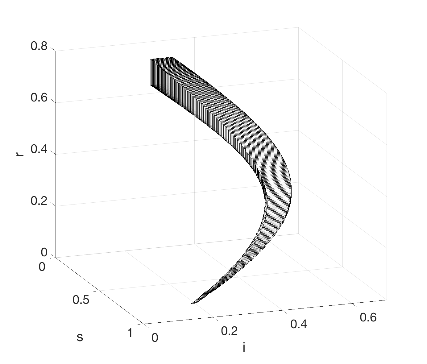
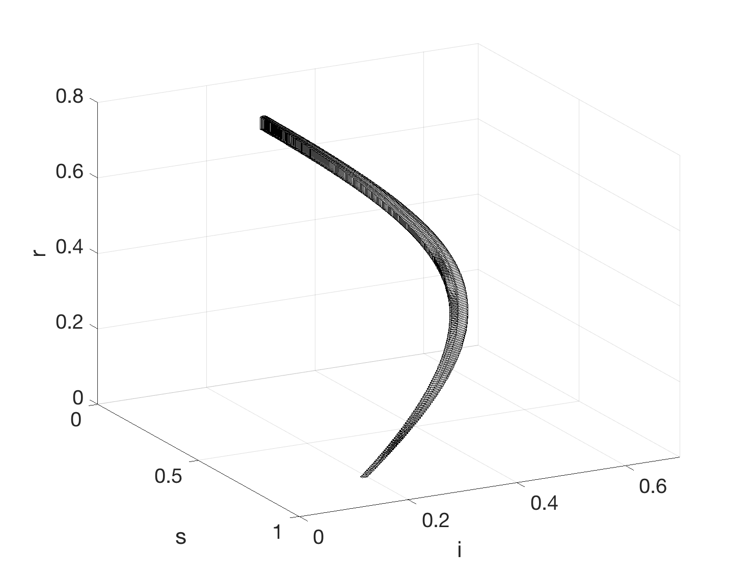
We used Sapo to compute the bounded time reachable set of the SIR model with different configurations. At first, with parameters $\displaystyle\beta=0.34,\gamma=0.05$, and set of initial conditions $\displaystyle s_{0}\in[0.79,0.80],i_{0}\in[0.19,0.20]$, and $\displaystyle r_{0}\in[0.00,0.00]$, we computed in $\displaystyle 0.12$s the reachable set for 300 steps using a single box (see Figure 2(a)). Then, by adding two surrounding parallelotopes to the set of initial conditions, we obtained in $\displaystyle 2.83$s a bundle-based flowpipe that better over-approximates the reachable set (see Figure 2(b)). Notice how, for the same initial set, the bundle-based flowpipe is more accurate than the box-based one.

(a) Box-based

(b) Bundle-based

Figure 2: Reachable sets of SIR model (300 steps)

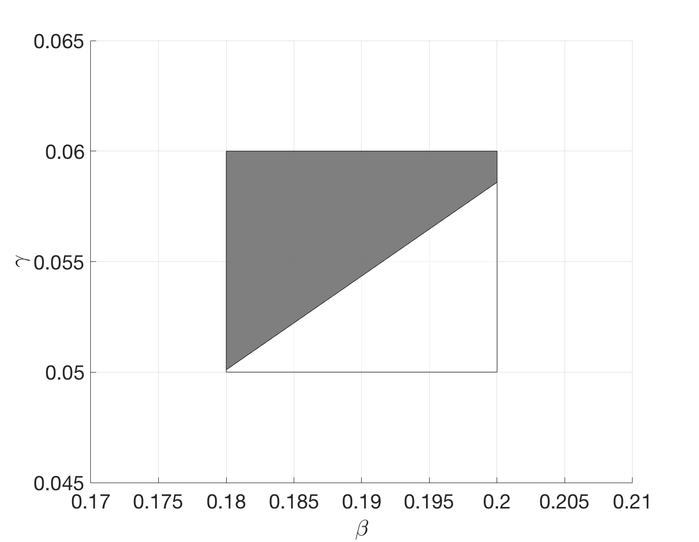
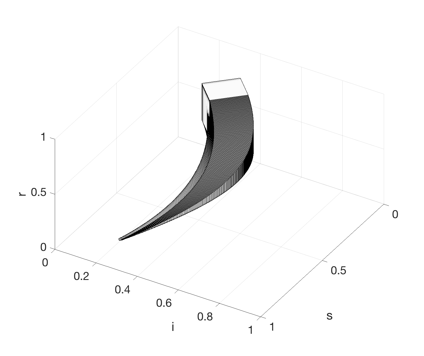
Sapo can also be used to synthesize sets of valid parameters. For instance, considering the set of initial conditions $\displaystyle s_{0}\in[0.79,0.80]$, $\displaystyle i_{0}\in[0.19,0.20]$, and $\displaystyle r_{0}=[0.00,0.00]$, and the initial set of parameters $\displaystyle\beta\in[0.18,0.20]$ and $\displaystyle\gamma\in[0.05,0.06]$, we can ask Sapo to refine the parameter set so that the STL formula $\displaystyle G_{[50,100]}(i\leq 0.44)$ holds. Figure 3(a) shows the original parameter set (in white) and the synthesized one (in gray) computed in $\displaystyle 0.83$s, while Figure 3(b) depicts the evolution of the system under the synthesized parameter set.

(a) Synthesized parameters

(b) Constrained evolution

Figure 3: Parameter synthesis of SIR model ($\displaystyle G_{[50,100]}(i\leq 0.44)$)

We evaluated both Sapo’s reachability and parameter synthesis algorithms on several dynamical systems [11, 6, 7, 10, 12]. We computed the reachable sets of biological models, such as SIR (3d) or a honeybees nest choice model (5d), or of a quadrotor drone (17d) (see Appendix A), and synthesized parameters of epidemic systems, such as SIR (3d, 2params), influenza (4d, 2params), Ebola (5d, 4params), and SARS (6d, 4params) (see Appendix B).

V Conclusion

V-A Related Work

In the last two decades numerous tools have been developed for the reachability analysis of linear dynamical system and hybrid automata. Some examples are SpaceEx [14], HyTech [15], or d/dt [3]. Unlike for the linear case, not many tools for the nonlinear analysis are available. Some tools, such as Breach [9], S-TaLiRo [2], or C2E2 [13] address nonlinearity using a finite number of simulations. Tools that directly deal with nonlinear reachability are dReach [16] and Flow*[5]. The latter is probably the closest tool to Sapo in terms of both problem formulation and provided results. The main difference between Flow* and Sapo is that the first produces flowpipes grouping collections of Taylor models, while the second produces a collection of polytopes computed using Bernestein coefficients. Another difference is that Flow* considers hybrid automata, while Sapo, at the moment, focuses only on dynamical systems.

V-B Future Developments

Sapo is still under development. As future work, we will extend the reachability computation to polynomial hybrid automata, where invariants and guards need to be considered. An interesting aspect of operations on parallelotope bundles is that they can be easily parallelized. It could be interesting to implement a parallel version of the tool and investigate its scalability. Finally, a comparison with the available tools for nonlinear reachability is on our schedule.

Appendix A Reachability

Model	Vars	Dir/Temps	Steps	Time
SIR [5]	2	4/2	25	0.24
		3/1	60	0.12
		6/4	60	2.83
Nest choice [1]	5	5/1	1500	26.90
		7/3	1500	81.27
Quadcopter [2]	17	17/1	300	17.74
		18/2	300	39.07

TABLE I: Reachability computation benchmark

Table I reports the evaluation of Sapo’s reachability computation algorithm. The tool has been evaluated on three nonlinear systems: the SIR epidemic model [5], a honeybees site choice model [1] describing the mechanism adopted by a swarm of honeybees to choose one among two different nest-sites, and a quadrotor drone model [2] characterizing both the drone and its controller dynamics. Each system has been tested on different combinations of number of directions and templates. The table reports the dimension of the system (i.e., the number of variables), the number of directions and templates used for the parallelotope bundle, the total number of reachability steps, and the computation times expressed in seconds.

Appendix B Parameter Synthesis

The scalability of the parameter synthesis algorithm has been studied in terms of system dimension (Section B-A) and specification’s length (Section B-B).

B-A Benchmark 1

Model	Vars	Params	Spec	Time
SIR [5]	3	2	$\displaystyle\mathcal{G}_{[10,30]}(i\leq 0.68)$	0.10
			$\displaystyle\mathcal{G}_{[20,50]}(i\leq 0.50)$	0.65
Influenza [4]	4	2	$\displaystyle\mathcal{G}_{[0,50]}(i\leq 0.43)$	6.27
Ebola [3]	5	4	$\displaystyle(i\leq 200)\mathcal{U}_{[6,10}(q\leq 20)$	0.10
			$\displaystyle(q\leq 40)\mathcal{U}_{[10,15]}(i\leq 270)$	0.14
			$\displaystyle(q\leq 50)\mathcal{U}_{[5,15]}(e>100\vee q>25)$	0.14

TABLE II: Parameter synthesis benchmark (scalability in system’s dimension)

Table II reports the evaluation considering models of increasing dimension. We considered three nonlinear dynamical systems: the SIR model [5], a simplification of the influenza model presented in [4], and a variation of the model describing the Ebola outbreak in Congo 1995 and Uganda 2000 exposed in [3]. For each model we considered different specifications. The table reports the dimension of the system, the numbers of synthesized parameters, the considered STL specification, and the computation time expressed in seconds.

B-B Benchmark 2

$\displaystyle a$	$\displaystyle b$	$\displaystyle\phi_{1}$	$\displaystyle\phi_{2}$	$\displaystyle\phi_{3}$
5	15	0.20 (11)	0.15 (7)	0.14 (4)
5	20	0.35 (16)	0.24 (11)	0.21 (4)
5	30	0.82 (26)	0.55 (21)	0.36 (4)
5	50	2.63 (46)	1.65 (41)	0.80 (4)
5	100	-	10.95 (91)	1.69 (4)
5	125	-	-	1.69 (4)
15	20	0.29 (6)	0.22 (4)	0.19 (0)
20	30	0.64 (11)	0.45 (11)	0.35 (0)
30	50	1.88 (21)	1.27 (21)	0.78 (0)
50	100	13.00 (51)	6.89 (51)	1.72 (0)
100	200	-	-	1.66 (0)
(a) Increasing until interval.

N	$\displaystyle\phi^{N}_{1}$	$\displaystyle\phi^{N}_{2}$	$\displaystyle\phi^{N}_{3}$
1	0.11 (5)	0.14 (2)	0.13 (4)
2	0.26 (9)	0.36 (7)	0.29 (3)
3	0.48 (13)	0.69 (12)	0.50 (3)
4	0.74 (17)	1.09 (17)	0.70 (3)
5	1.10 (21)	1.61 (22)	1.01 (3)
6	1.50 (25)	2.28 (27)	1.20 (3)
7	1.97 (29)	3.05 (32)	1.65 (3)
8	2.59 (33)	3.97 (37)	1.81 (3)
9	3.23 (37)	5.06 (42)	2.16 (3)
10	4.98 (42)	6.70 (47)	2.56 (3)
15	10.33 (61)	11.80 (62)	4.85 (3)
16	11.75 (65)	15.98 (67)	5.43 (3)
17	-	-	5.97 (3)
(b) Nesting until.

TABLE III: Parameter synthesis benchmark (scalability in specification’s size). Times and computed polytopes per refinement. $\displaystyle\phi_{1}\equiv(i\leq 200)\mathcal{U}_{[a,b]}(q\leq 20)$, $\displaystyle\phi_{2}\equiv(q\leq 40)\mathcal{U}_{[a,b]}(i\leq 270)$, $\displaystyle\phi_{3}\equiv(q\leq 50)\mathcal{U}_{[a,b]}(e>100\vee q>25)$.

For the second evaluation of the parameter synthesis algorithm we considered the six dimensional Ebola model [3] and we synthesize four of its controllable parameters over different specifications. Let $\displaystyle\phi_{1}\equiv(i\leq 200)\mathcal{U}_{[a,b]}(q\leq 20)$, $\displaystyle\phi_{2}\equiv(q\leq 40)\mathcal{U}_{[a,b]}(i\leq 270)$, and $\displaystyle\phi_{3}\equiv(q\leq 50)\mathcal{U}_{[a,b]}(e>100\vee q>25)$ be three STL specifications. Table IIIa reports the evaluations when stretching the time intervals $\displaystyle[a,b]$ of the specifications $\displaystyle\phi_{1},\phi_{2}$, and $\displaystyle\phi_{3}$. As second evaluation, we nested several until on the (most critical) right hand side. For instance, the double nesting of $\displaystyle\phi_{1}$ is $\displaystyle\phi^{N}_{1}\equiv(I(t)\leq 200)\mathcal{U}{[6,10]}((I(t)\leq 200)\mathcal{U}{[6,10]}(Q(t)\leq 20))$ with $\displaystyle N=2$. Table IIIb reports the running times and the number of obtained parameter sets.

References

- [1] Sapo. Available at http://www.eecs.berkeley.edu/~tommasodreossi/sapo/.
- [2] Y. Annpureddy, C. Liu, G. Fainekos, and S. Sankaranarayanan. S-taliro: A tool for temporal logic falsification for hybrid systems. In Tools and Algorithms for the Construction and Analysis of Systems, TACAS, pages 254–257, 2011.
- [3] E. Asarin, T. Dang, and O. Maler. The d/dt tool for verification of hybrid systems. In Computer Aided Verification, CAV, pages 365–370, 2002.
- [4] G.T. Cargo and O. Shisha. The Bernstein form of a polynomial. In Journal of Research, pages 79–81, 1966.
- [5] X. Chen, E. Ábrahám, and S. Sankaranarayanan. Flow*: An analyzer for non-linear hybrid systems. In Computer Aided Verification, CAV, pages 258–263, 2013.
- [6] T. Dang, T. Dreossi, and C. Piazza. Parameter synthesis using parallelotopic enclosure and applications to epidemic models. In Hybrid Systems and Biology, HSB, pages 67–82, 2014.
- [7] T. Dang, T. Dreossi, and C. Piazza. Parameter synthesis through temporal logic specifications. In International Synmposium on Formal Methods, FM, pages 213–230, 2015.
- [8] T. Dang and R. Testylier. Reachability analysis for polynomial dynamical systems using the Bernstein expansion. Reliable Computing, 17(2):128–152, 2012.
- [9] A. Donzé. Breach, a toolbox for verification and parameter synthesis of hybrid systems. In Computer Aided Verification, CAV, pages 167–170, 2010.
- [10] T. Dreossi. Reachability Computation and Parameter Synthesis for Polynomial Dynamical Systems. PhD thesis, University of Udine and Joseph Fourier University, 2016.
- [11] T. Dreossi and T. Dang. Parameter synthesis for polynomial biological models. In Hybrid Systems: Computation and Control, HSCC, pages 233–242, 2014.
- [12] T. Dreossi, T. Dang, and C. Piazza. Parallelotope bundles for polynomial reachability. In Hybrid Systems: Computation and Control, HSCC, pages 297–306, 2016.
- [13] P. S. Duggirala, M. Potok, S. Mitra, and M. Viswanathan. C2E2: a tool for verifying annotated hybrid systems. In Hybrid Systems: Computation and Control, HSCC, pages 307–308, 2015.
- [14] G. Frehse, C. Le Guernic, A. Donzé, S. Cottont, R. Ray, O. Lebeltel, R. Ripado, A. Girard, T. Dang, and O. Maler. SpaceEx: Scalable verification of hybrid systems SpaceEx: Scalable verification of hybrid systems In Computer Aided Verification, CAV, pages 379–395, 2011.
- [15] T. A. Henzinger, P. Ho, and H. Wong-Toi. HyTech: A model checker for hybrid systems. In Computer Aided Verification, CAV, pages 460–463, 1997.
- [16] S. Kong, S. Gao, W. Chen, and E. Clarke. dreach: -reachability analysis for hybrid systems. In Tools and Algorithms for the Construction and Analysis of Systems, TACAS, pages 200–205, 2015.
- [17] O. Maler and D. Nickovic. Monitoring temporal properties of continuous signals. In Formal Techniques, Modelling and Analysis of Timed and Fault-Tolerant Systems, pages 152–166, 2004.
- [1] N. F. Britton, N. R. Franks, S.C. Pratt, and T. D.Seeley. Deciding on a new home: how do honeybees agree? In Royal Society of London B: Biological Sciences, pages 1383–1388, 2002.
- [2] A. E. Carrilho da Cunha. Benchmark: Quadrotor Attitude Control. In Applied Verification for Continuous and Hybrid Systems, ARCH, 2015.
- [3] G. Chowell, N. W. Hengartner, C. Castillo-Chavez, P. Fenimore, and J. M. Hyman. The basic reproductive number of Ebola and the effects of public health measures: the cases of Congo and Uganda. In Journal of Theoretical Biology, 2004.
- [4] P. A. González-Parra, S. Lee, L. Velazquez, and C. Castillo-Chavez. A note on the use of optimal control on a discrete time model of influenza dynamics. In Mathematical Biosciences and Engineering, pages 183–197, 2011.
- [5] W. Kermack, O. William, and A. G. McKendrick. A contribution to the mathematical theory of epidemics. In Royal Society of London A: Mathematical, Physical and Engineering Sciences, pages 700–721, 1927.