Foreground Bias From Parametric Models of Far-IR Dust Emission

Abstract

We use simple toy models of far-IR dust emission to estimate the accuracy to which the polarization of the cosmic microwave background can be recovered using multi-frequency fits, if the parametric form chosen for the fitted dust model differs from the actual dust emission. Commonly used approximations to the far-IR dust spectrum yield CMB residuals comparable to or larger than the sensitivities expected for the next generation of CMB missions, despite fitting the combined CMB $+$ foreground emission to precision 0.1% or better. The Rayleigh-Jeans approximation to the dust spectrum biases the fitted dust spectral index by $\Delta\beta_{d}=0.2$ and the inflationary B-mode amplitude by $\Delta r=0.03$. Fitting the dust to a modified blackbody at a single temperature biases the best-fit CMB by $\Delta r>0.003$ if the true dust spectrum contains multiple temperature components. A 13-parameter model fitting two temperature components reduces this bias by an order of magnitude if the true dust spectrum is in fact a simple superposition of emission at different temperatures, but fails at the level $\Delta r=0.006$ for dust whose spectral index varies with frequency. Restricting the observing frequencies to a narrow region near the foreground minimum reduces these biases for some dust spectra but can increase the bias for others. Data at THz frequencies surrounding the peak of the dust emission can mitigate these biases while providing a direct determination of the dust temperature profile.

1. Introduction

Polarization of the cosmic microwave background (CMB) provides a critical test for models of inflation. The primary signature is is a parity-odd curl component in the polarization on angular scales of a few degrees or larger (Kamionkowski, Kosowsky, & Stebbins, 1997; Seljak & Zaldarriaga, 1997). The amplitude of this “B-mode” signal depends on the inflationary potential

$$V^{1/4}=1.06\times 10^{16}~{}{\rm GeV}\left(\frac{r}{0.01}\right)^{1/4}$$ (1)

where $r$ is the power ratio of the tensor (gravitational) perturbations to scalar (density) fluctuations (Turner & White, 1996). If inflation results from Grand Unified Theory physics (energy $\sim 10^{16}$ GeV), the B-mode amplitude should be in the range 1 to 100 nK. Signals at this amplitude could be detected by a dedicated polarimeter, providing a critical test of a central component of modern cosmology.

Detecting the inflationary signal will be challenging. A primary concern is confusion from astrophysical foregrounds. We view the CMB through a screen of diffuse Galactic emission originating within different components of the interstellar medium. Figure 1 compares the inflationary B-mode signal to polarized Galactic foregrounds. Synchrotron emission from relativistic cosmic ray electrons accelerated in the Galactic magnetic field dominates the diffuse radio continuum at low frequencies. For a power-law distribution of cosmic ray energy $N(E)\sim E^{-p}$, the synchrotron intensity is also a power law,

$$I_{s}(\nu)=A_{s}\left(\frac{\nu}{\nu_{s}}\right)^{\beta_{s}},$$ (2)

where $\nu$ is the observing frequency, $\beta_{s}=(1-p)/2$ is the spectral index, and $A_{s}$ is the amplitude defined relative to reference frequency $\nu_{s}$ (Rybicki & Lightman, 1979). The measured values $2.6<p<3.2$ for the cosmic ray energy spectrum correspond to synchrotron spectral index $-1.1<\beta_{s}<-0.8$, in reasonable agreement with radio data (Strong et al., 2007; Jaffe et al., 2011; Kogut, 2012; Bennett et al., 2013; Planck collaboration, 2015a). The synchrotron spectrum may contain additional features (curvature, spectral break), but evidence for such features is restricted to frequencies below 20 GHz and is not considered here.

Dust is the dominant foreground at high frequencies. Dust grains in the interstellar medium absorb optical and UV photons and re-radiate the energy in the far-infrared. The resulting spectrum is often empirically modeled as a sum of modified blackbodies with power-law emissivities,

$$I_{d}(\nu)=\sum_{i}\epsilon_{i}B_{\nu}(T_{i})\left(\frac{\nu}{\nu_{d}}\right)^{\beta_{d\,i}}$$ (3)

where $B_{\nu}(T)$ is the Planck intensity at temperature $T$, and the emissivity $\epsilon$ and spectral index $\beta_{d}$ are defined at reference frequency $\nu_{d}$. Fitting the high-latitude dust cirrus to a single modified blackbody returns values $T_{d}~{}=~{}20$ K and $\beta_{d}=1.6$ (Planck collaboration, 2015b).

The B-mode signal is fainter than the Galactic foregrounds at all frequencies. Current measurements limit primordial B-modes to amplitude $r<0.07$ at 95% confidence (BICEP2/Keck and Planck Collaborations, 2015). Distinguishing primordial B-modes from Galactic foregrounds at this level requires subtracting the foregrounds to few percent accuracy or better. The next generation of CMB polarimeters anticipates sensitivities $r<0.001$. Measurements at this level require foreground subtraction with sub-percent accuracy.

Despite their importance, diffuse Galactic foregrounds at millimeter wavelengths are poorly constrained. The observed dust emission depends on a number of factors including the grain size distribution, chemical and physical composition of the dust grains, competing emission mechanisms within a grain, and the three-dimensional distribution of the dust population irradiated by the stellar UV/optical field. None of these are known in detail. Lacking a detailed physical model, CMB analyses typically use a purely phenomenological model for the dust, treating it as the sum of one or two modified blackbody components along each line of sight. In this paper, we use simple extensions to commonly used models of far-IR dust emission to estimate the systematic error (bias) in the B-mode amplitude $r$ due to the use of such phenomenological models.

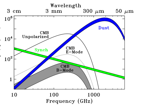
Figure 1.— Frequency spectra of the CMB and polarized foregrounds. The grey band shows 0.01$<$$r$$<$0.1 for the primordial inflation signal. Colored bands show the synchrotron and dust foregrounds for the cleanest 50% and 75% of the sky. The inflationary signal is fainter than Galactic foregrounds at all frequencies, requiring accurate models for foreground subtraction.

2. Dust Emission Models

A common approximation treats far-IR dust emission as a modified blackbody at a single well-defined temperature $T_{d}$ (Eq. 3). Applied to the Planck polarization data, the single-temperature model yields dust temperature $19.6\pm 0.8$ K with spectral index $1.59\pm 0.02$ (Planck collaboration, 2015b). However, data at higher frequencies show that roughly 4% of the far-IR power resides in a component consistent with a colder temperature near 10 K (Wright et al., 1991; Reach et al., 1995; Dwek et al., 1997; Finkbeiner, Davis, & Schlegel, 1999; Meisner & Finkbeiner, 2015). The origin of this component is unknown. The sum of two blackbodies can not be modeled to arbitrary precision as a third blackbody: the single-temperature model is at best an approximation to the underlying dust spectrum.

The two-component modified blackbody model fits the far-IR dust intensity along each line of sight to the superposition of emission from components at two discrete temperatures. This, too, can only approximate the underlying spectrum. The dust emission spectrum represents a balance between optical/UV power absorbed by each grain and subsequently re-radiated in the far-infrared. It thus depends on both the absorption and emission properties of individual dust grains as well as the grain size and the stellar radiation field illuminating each grain. All of these will vary within the interstellar medium. The stellar radiation field must vary as individual dust grains lie at different distances from individual stellar sources. Differences in the physical properties of dust grains yield additional temperature differences, with carbonaceous grains systematically colder than silicates (see, e.g., Zubko, Dwek, and Arendt (2004); Draine and Li (2007); Draine and Fraisse (2009)). Transient heating of small grains drives further temperature variation, even within a homogeneous dust population illuminated by a uniform stellar radiation field.

Figure 2.— Far-IR dust opacity vs temperature for several toy models of far-IR dust emission. (Top) Two-component modified blackbody emission for which the dust opacity is non-zero at exactly two temperatures. (Middle) A broader distribution with two peaks smoothed by a Gaussian distribution. (Bottom) Distribution with a single low-temperature peak and an extended “tail” toward higher temperatures, approximating a population with transient heating.

Systematic differences between the spectrum of the diffuse dust cirrus and the parametric models used to describe this emission will bias foreground subtraction for CMB observations. Models of foreground emission sufficient for E-mode or unpolarized analyses can prove inadequate at the higher accuracy required for B-mode analysis. We quantify the extent to which specific choices for the dust parameterization bias the fitted CMB terms using toy models of dust emission. We begin with simple models of far-IR emission that have been used for CMB fitting (Rayleigh-Jeans approximation, one- and two-component modified blackbodies), then extend the parameterization to include a distribution in dust temperature (Figure 2). The simplest extension beyond the two-temperature model retains two temperature peaks, but broadens the distribution using a Gaussian smoothing to include emission at intermediate temperatures as well. We additionally consider a model with a single peak at low temperatures plus an extended “tail” to higher temperatures to approximate the effect of transient heating. For both the Gaussian and transient models, we adjust the relative amplitudes of the warm and cold components so that emission from the cold component remains at the observed 3.7% of the power from the warm component while forcing the combined dust emission to match the intensity of Planck polarized dust model at 353 GHz. Finally, we consider a model in which the dust spectral index varies with frequency, flattening the spectrum at lower frequencies. Such “running” of the spectral index is an expected characteristic of two-level emission in disordered dust grains (Mény et al., 2007; Paradis et al., 2011).

Although not intended to represent in detail any specific physical model of far-IR dust emission, the toy models used here capture sufficient features of leading models to examine the implications for simple parametric dust models. Other forms for the dust emission are possible. So-called “anomalous microwave emission” is a significant contribution to the unpolarized intensity at frequencies below 90 GHz (Kogut et al., 1996; Gold et al., 2011; Planck collaboration, 2011; Génova-Santos et al., 2015) and is thought to result from a population of small, spinning dust grains (Draine and Lazarian, 1998; Ali-Haïmoud et al., 2009; Hoang et al., 2010). Anomalous microwave emission is not known to be polarized, with upper limits to the fractional polarization at the sub-percent level (Génova-Santos et al., 2015). Dust containing magnetic material could also emit through thermal fluctuations of the grain magnetization, which would have comparable polarization to thermal dust emission but would differ significantly from a power-law emissivity (Draine and Hensley, 2012).

3. Simulations

Several authors have estimated the sensitivity and possible systematic bias in $r$ resulting from foreground contamination of CMB observations (Fantaye et al., 2011; Remazeilles et al., 2016). These analyses only examine simple single-temperature dust models and are limited to choices of observing frequencies and instrumental sensitivity matched to specific CMB missions. Here we focus on the bias resulting from the unknown dust spectra, with a broader range of plausible dust emission models not limited to instrument-specific observing frequencies.

We evaluate the CMB and foreground emission using noiseless simulations. All simulations adopt a power-law model (Eq. 2) with $\beta_{s}=-1.05$ for the synchrotron spectral dependence but use different toy models for the dust. Rather than simulate a specific instrument configuration, we evaluate the simulations using frequency channels spaced every 10 GHz starting at 30 GHz and extending to some maximum frequency (typically 500 GHz). The number of frequency channels is thus much larger than the number of fitted parameters so that the results do not depend on details of the frequency basis. We normalize the foreground emission in Stokes $Q$ and $U$ to match the Planck polarized foreground maps at 30 GHz for synchrotron emission and 353 GHz for dust (Planck collaboration, 2015a). The dust normalization is thus fixed by observation and does not depend on assumptions for the fractional polarization of the dust emission. We degrade the maps to a common HEALPIX resolution NSIDE=256 (Górski et al., 2005) and fit the superposed emission in each pixel outside the Planck HFI polarization mask to combination of CMB, synchrotron, and dust emission where the parametric form of the fitted dust model now differs from the input. The fit minimizes the weighted sky residual

$$\Gamma^{2}=\sum_{i}\left(\frac{I_{\rm fit}-I_{\rm input}}{W}\right)^{2}_{i}.$$ (4)

Although the input model has no noise contribution, we weight each frequency channel by the inverse of the combined input sky intensity, $W=I_{\rm input}$, so that the fit is not dominated by channels where the foregrounds are much brighter than the CMB. This approximates common practice for CMB observations, where the sensitivity in each channel is chosen to produce equal signal-to-noise ratio at all frequencies. Other choices for channel weights are possible (for instance, uniform weight at all frequencies). The results do not depend sensitively upon the choice of weights. The fitted $Q$ and $U$ amplitudes for the CMB component in each pixel are then used in a spherical harmonic analysis to determine the amplitude of the B-mode signal, which we compare to the simulation input to determine the bias in $r$. Note that this automatically includes the typical 2:1 ratio of E-mode to B-mode power observed for the polarized dust foreground.

Figure 3.— Intensity ratio of power-law dust emission normalized to a single-temperature modified blackbody with $T_{d}=20$K (see text). The Rayleigh-Jeans approximation fails at the few-percent level for frequencies above 20 GHz and dust temperatures appropriate for the diffuse dust cirrus.

4. CMB Bias from Parametric Dust Models

A commonly used technique for foreground identification and subtraction is parametric modeling, in which measurements of the sky intensity in multiple frequency channels are modeled as the sum of CMB and foreground components specified by their frequency dependence. We evaluate noiseless simulations using different parametric forms for the fitted dust model to quantify the dependence of CMB residuals on the choice of input versus fitted dust models.

4.1. Rayleigh-Jeans Approximation

At sufficiently low frequencies, dust emission may be approximated as a power law in intensity,

$$I_{d}(\nu)=a_{d}\left(\frac{\nu}{\nu_{d}}\right)^{2+\beta_{d}}~{}.$$ (5)

This Rayleigh-Jeans approximation has seen considerable use for modeling the dust contribution to CMB measurements at frequencies from 22 GHz to 410 GHz (Kogut et al., 1996; Masi et al., 2001; Ponthieu et al., 2005; Paladini et al., 2007; Dupac, 2009; Bennett et al., 2013). Although appropriate for the sensitivity levels of these analyses, reliance on the Rayleigh-Jeans approximation will in general bias both the fitted dust parameters and the estimated CMB amplitudes. The Rayleigh-Jeans approximation is valid in the limit $x~{}=~{}h\nu/kT_{d}\ll~{}1$ where $h$ is Planck’s constant, $k$ is Boltzmann’s constant, and $T_{d}$ is the dust temperature. For dust at temperature $T_{d}=20$ K, $x=0.24$ at 100 GHz and does not fall below 0.05 until $\nu<21$ GHz. At the frequencies $\nu>20$ GHz used by most CMB missions, the spectral curvature of the Planck function $B_{\nu}(T)$ can not be approximated by a power-law to percent-level accuracy. Figure 3 compares dust emission from a single modified blackbody (Eq. 3) with $T_{d}=20$ K and $\beta_{d}=1.6$ to the best-fit Rayleigh-Jeans approximation. The curvature of the modified blackbody relative to a power-law fit is apparent at the few-percent level.

Use of the Rayleigh-Jeans approximation in multi-component foreground estimation will bias estimates of the individual components. Figure 4 compares the input and fitted sky models for noiseless simulations ($\S$3) where the input dust consists of a modified blackbody with $T_{d}=19.6$ K and $\beta_{d}=1.59$. Fitting the simulated sky over the frequency range 30–140 GHz using the Rayleigh-Jeans approximation for the dust component matches the superposed input spectra to precision $\Delta I/I<0.04$%, but biases both the fitted dust and CMB components. The differential curvature of the modified blackbody dust input compared to the power-law output model over-estimates the dust emission by 15% at frequencies near the foreground minimum at 70 GHz. The best-fit spectral indices are displaced from the input values, with fitted values $\beta_{s}=-1.04$ for synchrotron and $\beta_{d}=1.33$ for dust. The shift in dust spectral index produced by the Rayleigh-Jeans approximation at low frequencies mimics the flattening seen in the two-level-system model although in this case it is entirely an artifact of the approximation. The fitted model returns a false CMB term with (negative) amplitude 80 nK, comparable to a B-mode signal at level $r=0.03$ for the multipole range $50<\ell<200$ targeting the “recombination bump.”

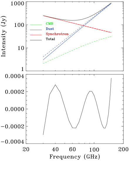
Figure 4.— Input spectra compared to best-fit model when the input dust consists of a single modified blackbody but the fitted model assumes the power-law Rayleigh-Jeans approximation. (Top) Input spectra (solid lines) and best-fit model (dashed lines). The input has synchrotron and dust but no CMB, with foreground amplitudes at the median brightness of the polarized Planck foreground model. (Bottom) Fractional residual $\Delta I/I$ for the combined spectra. Although the multi-component fit matches the combined sky spectrum to sub-percent precision, the Rayleigh-Jeans approximation biases the recovered amplitudes and spectral index values, generating a false CMB term at level $r\sim 0.03$.

4.2. One-component Modified Blackbody

The simplest model beyond the Rayleigh-Jeans approximation treats the dust spectrum as modified blackbody at a single temperature with power-law emissivity. A single-temperature model allows fits across a wide frequency range but can yield biased results if the far-IR dust emission differs systematically from the model.

One such effect, present even if the dust were dominated by just one temperature component, results from errors in the dust temperature. Measurements at millimeter wavelengths may lack either the frequency coverage or sensitivity for direct estimation of the dust temperature in each pixel, relying instead on measurements at higher frequencies near the peak dust intensity or on spatial averaging across larger regions on the sky. Data from the FIRAS, DIRBE, and Planck missions show spatial variation of 3.5 K in the dust temperature across the sky (Finkbeiner, Davis, & Schlegel, 1999; Planck collaboration, 2015a). Substituting a mean dust temperature into multi-frequency foreground models will bias the fitted components if the dust temperature within any pixel differs from the supplied mean value. Figure 5 illustrates the effect. As before, we fit a noiseless superposition of synchrotron and dust emission with no CMB term, evaluated at frequencies 30–500 GHz using a model consisting of synchrotron, dust, and CMB. The input dust model consists of a single modified blackbody with $T_{d}=19.6$K and $\beta_{d}=1.59$. The fitted dust model uses the same modifed blackbody parameterization as the input, but with dust temperature $T_{d}$ offset by $\Delta T$ with respect to the input model. The fitted parameters are thus the synchrotron amplitude and spectral index, the dust amplitude and spectral index, and the CMB amplitude. Differences between the true dust temperature and the temperature assumed for the model result in a biased CMB component, with a 1K dust temperature offset corresponding to a CMB amplitude of 20 nK. Parametric fits that use an externally supplied value for the dust temperature generate a bias in the fitted CMB amplitude if the assumed dust temperature in each pixel differs from the true value. Keeping this term below the 3 nK amplitude corresponding to $r=0.001$ requires knowledge of the dust temperature in each pixel accurate to 0.15 K or better.

Figure 5.— Bias in fitted CMB component when both the input dust and the fitted model follow a single-temperature modified blackbody parameterization, but the fitted dust temperature differs from the true dust temperature.

4.3. Two-Component Modified Blackbody

Data at THz frequencies where dust emission peaks show that 3.7% of the far-IR dust power is contained in a second, colder component at temperature 8–12 K (Reach et al., 1995; Finkbeiner, Davis, & Schlegel, 1999; Meisner & Finkbeiner, 2015). The superposition of two blackbodies at different temperatures cannot be modeled to arbitrary accuracy as a single blackbody at a third temperature. The existence of a cold component in the interstellar dust cirrus will necessarily bias CMB fits that ignore this component.

We evaluate the effect by fitting a simulated sky spectrum over the frequency range 30 – 500 GHz using a superposition of synchrotron and dust emission with no CMB term. The dust emission in each pixel is a superposition of two modified blackbody components: a warm component with temperature $T_{d}\sim 16$ K and spectral index $\beta_{d}=2.70$, plus a cold component with $T_{d}\sim 9$ K and $\beta_{d}=1.67$. The spectral index of each component is held constant over the entire sky, but the temperatures and relative amplitudes are derived for each pixel following Finkbeiner, Davis, & Schlegel (1999). The overall normalization of the combined dust emission in Stokes $Q$ and $U$ is set to match the Planck polarized dust model at 353 GHz. The fitted model assumes a superposition of synchrotron, dust, and CMB emission using a single modified blackbody (Eq. 3) for the dust, for a total of 9 free parameters in each pixel (Stokes $Q$ and $U$ amplitudes for the CMB, synchrotron, and dust plus the synchrotron spectral index, dust spectral index, and dust temperature). Figure 6 shows the B-mode power spectrum for the fitted CMB component. Fitting two-component dust to a single dust component creates CMB residuals with amplitude comparable to the inflationary B-modes $r=0.003$ at the recombination bump and $r=0.006$ at the reionization bump.

4.4. Multi-component Modified Blackbody

Section $\S$4.3 demonstrates that fitting two-temperature dust using a single-temperature model results in a bias $\Delta r>0.003$. Extending the fitted dust model to include a second component reduces this bias. As before, we quantify the bias using an input sky with power-law synchrotron plus dust emission derived from one of the toy models in Figure 2, fitting the simulated sky to a model with CMB, synchrotron, and modified blackbody dust with two temperature components. The model now has a total of 13 free parameters in each pixel: 8 parameters for the Stokes $Q$ and $U$ amplitudes of the CMB, synchrotron, warm dust, and cold dust components, plus an additional 5 free parameters (synchrotron spectral index, warm dust temperature and spectral index, cold dust temperature and spectral index) to determine the foreground spectra, which are assumed to be identical for Stokes $Q$ and $U$. The resulting model fits the two-component input exactly, and reduces the bias in the CMB solution for both the Gaussian and transient toy models. The biases depend somewhat on the detailed temperature distribution, but are typically of order 0.3 nK ($\Delta r\sim 1\times 10^{-4}$) for the two-Gaussian toy model and 2 nK ($\Delta r\sim 8\times 10^{-4}$) for the transient heating model.

Figure 6.— Power spectrum of CMB residuals created when a sky with modified blackbody dust with two temperature components is fit using a single-temperature modifed blackbody model. The thin dashed lines show inflationary models with $r=0.01$ and $r=0.001$ while the thin dotted line shows the lensing signal. Fitting two-tempeature dust with a single-temperature model creates CMB residuals large compared to $r=0.001$.

4.5. Two-Level Systems and Running Spectral Index

The models in $\S$4.2 – 4.4 treat the far-IR dust spectrum as a superposition of modified blackbody emission from components at different physical temperatures. The far-IR emission of interstellar dust grains is not well understood and could plausibly utilize different physical mechanisms. One example is the two-level system (TLS) emission model developed by Phillips (1972), Anderson et al. (1972), and Bösch (1978) and later extended to interstellar dust (Agladze et al., 1996; Mény et al., 2007; Paradis et al., 2011). Emission in this model is dominated by acoustic oscillations in a disordered charge medium and by hopping relaxation in a distribution of two-level tunneling states. The temperature-independent acoustic oscillations are the principal emission component at THz frequencies, while hopping relaxation adds an additional temperature-dependent component to flatten the spectrum at millimeter wavelengths.

The TLS model has several attractive features. It invokes solid-state physics to reproduce the observed anti-correlation between the dust temperature and spectral index derived from modified blackbody fits to the far-IR dust spectra (Dupac, 2003; Désert et al., 2008; Bracco et al., 2011; Planck collaboration, 2014). Emission from the tunneling component reproduces the excess emission observed at millimeter wavelengths without requiring a cold dust component. Spectral fits using COBE/FIRAS data show the TLS model to be a viable description of far-IR emission from interstellar dust (Paradis et al., 2011; Odegard et al., 2016).

A key feature of the TLS model is the progressive flattening of the spectrum toward lower frequencies. It may be approximated as a temperature-dependent “running” of the spectral index, $\beta_{d}=\beta_{d}(T,\nu)$. At dust temperatures $T_{d}=20$ K typical for the diffuse interstellar cirrus, the spectral index flattens from $\beta_{d}=2$ at THz frequencies to $\beta_{d}\sim 1$ at 30 GHz (see, e.g., Figure 6 of Paradis et al. (2011)).

The spectral flattening at frequencies below 500 GHz where CMB emission peaks can bias multi-component fits relying on simpler models of the far-IR dust emission. We quantify the bias in $r$ using a toy model of TLS dust. The toy model approximates the TLS emission using a running spectral index,

$$I_{d}(\nu)=\epsilon(\nu_{d})B_{\nu}(T)\left(\frac{\nu}{\nu_{d}}\right)^{\beta_{d}(T,\nu)}.$$ (6)

We adopt the input dust temperature for each sky pixel using the Planck single-temperature modified blackbody model, and interpolate $\beta_{d}(T,\nu)$ in frequency using data from Paradis et al. (2011) appropriate for the dust temperature at that pixel. The resulting spectrum is then normalized to the Planck polarized dust model at 353 GHz. We fit the superposed synchrotron and dust emission to a model with CMB, synchrotron, and dust using the same two-component modified blackbody as $\S$4.4 and evaluate the resulting CMB component to derive the bias in $r$. The two-component modified blackbody model reproduces the combined input sky well, with fractional residuals $\Delta I/I<10^{-6}$ for all frequencies between 30 GHz and 500 GHz. However, the best-fit sky includes a biased CMB component with typical bias $\Delta r=6\times 10^{-3}$.

Note that the noiseless simulations fit the foreground spectra independently for each pixel. Actual observations include instrument noise and typically fit some foreground parameters (temperature, amplitude) within each pixel while fitting others (spectral index) over larger regions of the sky. The biases above thus represent an optimistic limiting case where the signal to noise ratio allows fitting 13 free parameters within each pixel. Even for this optimistic case, biases can be present at amplitudes large compared to projected instrument sensitivities.

5. Discussion

Parametric modeling of the diffuse dust foreground can bias estimates of CMB polarization if the chosen dust model cannot adequately represent the true emission spectrum. For the commonly used one- or two-component modified blackbody models, the bias can exceed levels $\Delta r\sim{\rm few}\times 10^{-3}$, large compared to the sensitivities anticipated for the next generation of CMB instrumentation (Kogut et al., 2011; Matsumura et al., 2014; Delabrouille et al., 2015; Abazajian et al., 2015). Foreground bias at this level would represent a statistically significant error in derived cosmological parameters and (depending on the cosmology) could induce a false detection of the inflationary signal.

Several techniques may be employed to reduce this bias. One method is to restrict the observing bands to frequencies 30 GHz $<\nu<$ 250 GHz where the CMB is brightest compared to the combined synchrotron and dust foregrounds, thereby reducing the precision to which the foreground emission must be modeled. Parametric fitting over a restricted frequency range also reduces the effect of un-modeled spectral curvature present when the fitted spectral model differs from the true foreground spectra. However, the smaller foreground amplitudes within the restricted frequency range require correspondingly better sensitivity in foreground-dominated channels to identify and remove the foreground emission.

Figure 7.— Effect of restricted observing frequencies for parametric dust models. (Top) Bias $\Delta r$ caused by fitting a single-temperature modified blackbody dust model to a sky containing dust emission from the two-temperature, two-Gaussian, or transient heating toy models (see text). The best-fit value for $r$ changes sign when fitting the transient heating input. (Bottom) Residual between the input sky and best-fit model, evaluated at the highest observed frequency.

We quantify this trade by fitting simulated skies while varying the frequency range over which the fit is performed. The input sky consists of power-law synchrotron with spectral index $-1.05$ plus dust specified by either the two-temperature, two-Gaussian, or transient toy models from $\S$4.4. The fitted model includes CMB, synchrotron, and single-temperature modified blackbody dust for a total of 9 free parameters. We fit the simulated sky using 10 observing channels spaced logarithmically in frequency starting at 30 GHz, and vary the highest observed frequency from 150 GHz to 950 GHz to show the effect of extending observations into the brighter dust foreground at higher frequencies.

Figure 7 shows the results. For the two-temperature and two-Gaussian input models, the simulations show the expected pattern with the bias $\Delta r$ monotonically decreasing as the frequency range is restricted. Fitting a single modified blackbody to a toy model with a high-temperature tail shows a different pattern. When the fit is restricted to frequencies below 400 GHz, the single-component model under-estimates the dust emission and over-estimates the CMB. When the frequency range is extended to the higher frequencies where the warmer components dominate, the single-component model over-estimates the dust emission and under-estimates the CMB. The residual CMB term thus changes sign, creating a null for the special case where the frequency coverage extends just high enough that the dust residuals cancel. Note that, for the transient heating toy model, restricting the frequency coverage below 400 GHz actually increases the bias in $r$.

A second consideration for restricted frequency coverage is sensitivity. As the frequency coverage is restricted, the parametric models better reconstruct the superposed emission from the CMB and combined foregrounds. This is not the same as accurately reconstructing the CMB signal itself. For the noiseless simulations in this paper, we define a goodness-of-fit statistic $\Gamma$ using the rms difference between the intensities of the input sky and the best-fit model, summed over observing channels (Eq. 4). This fractional residual varies from $\Gamma=10^{-5}$ for fits restricted to frequencies $\nu<200$ GHz to $\Gamma=10^{-3}$ for fits extending to $\nu<950$ GHz and is nearly identical for all three toy models considered.

The toy models evaluated above yield non-trivial bias in $r$ despite fitting the combined sky emission to sub-percent precision. Since the functional form of far-IR dust emission is not known a priori, distinguishing between biased and unbiased fits requires channel sensitivities comparable to the residuals derived from plausible models of dust emission. The design of CMB missions typically includes one or more “guard channels” at higher frequencies where dust emission dominates. The bottom panel of Figure 7 shows the guard channel sensitivity required to distinguish these toy models,

$$\delta S=\Gamma~{}I_{\rm input}|_{\nu=\nu_{\rm max}},$$ (7)

evaluated as a function of the highest observing frequency. Since the highest observing frequency may extend to frequencies beyond the Wien cutoff in the CMB intensity, we present the sensitivity $\delta S$ in units of Rayleigh-Jeans temperature,

$$\delta T_{\rm RJ}=\delta S~{}\frac{\lambda^{2}}{2k}$$ (8)

where $k$ is Boltzmann’s constant and $\lambda$ is the observing wavelength.

Figure 7 illustrates the challenges for observations with restricted frequency coverage. A nine-parameter fit limited to observations at frequencies $\nu<250$ GHz most accessible to ground-based observations yields biases $\Delta r~{}>~{}10^{-3}$ despite fitting the combined sky emission to precision $\Gamma\sim 10^{-5}$. A statistical detection of this bias would require sub-nK channel sensitivities.

At least two solutions are possible. Fits with additional free parameters can better model the (unknown) dust spectrum, reducing the bias in the fitted CMB component. A 13-parameter model reduces the bias substantially ($\S$4.4) but would require at least 14 observing channels. Fitting multiple temperature components within a restricted frequency range may additionally lead to parameter degeneracies.

An alternative is to include observations at higher frequencies. Extending the observations to THz frequencies where the dust emission peaks provides discrimination among various dust models. For example, extending observations to 3 THz increases the residual between the input sky and best-fit model to 400 Jy sr^-1 for the TLS model and over 2000 Jy sr^-1 for the transient heating model. Differences at this level are readily detectable, providing statistical evidence for a poorly fitted model.

Observations at frequencies at or above the peak of the dust spectrum can additionally provide information on the actual dust temperature distribution, further discriminating between candidate dust models. Emission from dust components at successively higher temperatures will peak at successively higher frequencies (the well-known Wien displacement law); however, the superposed emission from multiple temperature components will typically show a single broad peak. One indicator of the temperature information within the superposed spectrum may be shown by Gram-Schmidt orthogonalization. We begin with a Planck spectrum at some minimum temperature $T_{\rm min}$, and construct orthogonal linear combinations from Planck spectra at successively higher temperatures to some maximum $T_{\rm max}$. Figure 8 shows the resulting orthogonal components for temperatures 8 K $<~{}T~{}<$ 24 K, evaluated at frequencies $\nu<5$ THz. There is relatively little spectral content at frequencies below 800 GHz, but well-separated peaks in the component spectra at higher frequencies.

Another way to evaluate the ability of THz observations to constrain the dust temperature distribution is to note that emission on the Rayleigh-Jeans side of the emission peak shows flatter spectral dependence compared to the exponential Wien cutoff at higher frequencies. Dust at temperatures $T_{d}>8$ K will peak at frequencies above 800 GHz, so it is not surprising to find most of the spectral content at frequencies above 800 GHz.

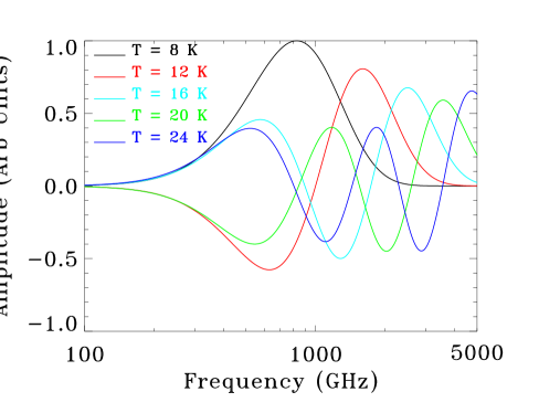
Figure 8.— Dust spectral components corresponding to different physical temperatures, derived from Gram-Schmidt orthogonalization of the individual Planck spectra at each temperature. The minimal spectral content at frequencies below 800 GHz makes it difficult for observations at low frequencies to distinguish multiple temperature components: most of the spectral content lies at frequencies above 1 THz.

6. Summary

Far-IR dust emission is complex. Variation in the chemical or physical composition of the dust grains or in the local stellar radiation field incident on each grain will drive variation in the physical temperature of the grains. Transient heating of individual grains drives further temperature variation, even for a homogeneous dust population illuminated by a uniform radiation field. Phenomenological models treating the far-IR emission spectrum as modified blackbody emission at one or two well-defined temperatures can only approximate the dust spectrum. Systematic differences between the actual emission spectrum and the simpler parametric forms used to model the emission will then bias both the recovered CMB and dust parameters.

We use toy models of far-IR dust emission to estimate the accuracy to which the polarization of the cosmic microwave background can be recovered if the parametric form chosen for the dust component of a multi-frequency fit differs from the actual dust emission. We generate noiseless simulations combining power-law synchrotron emission with toy models of dust emission, evaluate the combined emission at a set of observing frequencies spanning the minimum of the foreground spectra, then fit the resulting multi-frequency spectra to a superposition of synchrotron, dust, and CMB emission to derive the bias in CMB polarization. Differences between the input sky simulation and the parametric models used to fit the dust component yield CMB residuals comparable to or larger than the sensitivities expected for the next generation of CMB missions, despite fitting the combined sky emission to a precision $\Delta I/I$ of $10^{-3}$ or better.

The amplitude of the CMB residual depends on the complexity of the input dust model, the number of parameters used by the output dust model, and the frequency range over which the fit is performed. Although dust at millimeter wavelengths is often modeled as a modified blackbody at a single, well-defined temperature, the spectrum is known to be more complex. Observations at higher frequencies show excess emission with respect to the single-temperature modified blackbody dust model. The excess is consistent with emission from a second, colder dust component. Simulations with input skies containing either the two-component modified blackbody dust model or emission from extended temperature distributions but fit to a nine-parameter model with a single-temperature modified blackbody dust component consistently yield CMB residuals $\Delta r>0.003$ for the inflationary B-mode amplitude. Restricting observations to frequencies 30 GHz $<~{}\nu~{}<$ 250 GHz where the CMB is brightest relative to the foregrounds reduces the bias for some of the two-component input model, but actually increases the bias when the input model assumes a continuous distribution of dust emissivity extending to higher temperatures.

Adding additional free parameters to the output dust model reduces the CMB bias in certain cases. A 13-parameter output model fitting two modified blackbody dust components reproduces the two-component input model exactly, and reduces CMB bias by an order of magnitude for input models with extended temperature distributions. However, the 13-parameter model fails when the input sky contains dust with a running spectral index. Such a running index is consistent with observations and is expected for dust emission originating from two-level systems within the disordered medium of interstellar dust grains. A 13-parameter fit to the TLS model showed CMB residuals $\Delta r=6\times 10^{-3}$ despite fitting the combined CMB$+$foreground emission at frequencies $\nu<500$ GHz to precision $\Delta I/I<10^{-6}$.

Observations at THz frequencies surrounding the peak of dust emission can mitigate these biases. Extending parametric fits over a broader frequency range increases the residuals when the parametric form of the fitted model poorly matches the actual sky. At THz frequencies, the output-input dust residual for the toy models had readily detectable values 400–2000 Jy sr^-1, allowing statistical detection of poorly fitted models. Observations at THz frequencies would also allow direct determination of the dust temperature profile, informing fits at lower frequencies.

References

- Abazajian et al. (2015) Abazajian, K. N., Arnold, K., Austermann, J., et al., 2015, APh, 63, 66
- Agladze et al. (1996) Agladze, N. I., Sievers, A, J., Jones, S. A., et al., 1996, ApJ, 462, 1026
- Ali-Haïmoud et al. (2009) Ali-Haïmoud, Y., Hirata, C. M., & Dickinson, C., 2009, MNRAS, 395, 1055
- Anderson et al. (1972) Anderson, P. W., Halperin, B. I., & Varma, C. M., 1972, PMag, 25, 1
- Bennett et al. (2013) Bennett, C. L., Larson, D., Weiland, J. L., et al., 2013, ApJS, 208, 20
- BICEP2/Keck and Planck Collaborations (2015) BICEP2/Keck and Planck Collaborations, 2015, Phys. Rev. Lett., 114, 101301
- Bösch (1978) Bösch, M.A., 1978, Phys. Rev. Lett., 40, 879
- Bracco et al. (2011) Bracco, A., Cooray, A., Veneziani, M., et al. 2011, MNRAS, 412, 1151
- Delabrouille et al. (2015) Delabrouille, J (2015) http://hdl.handle.net/11299/169642.
- Désert et al. (2008) Désert, F.-X., Macías-Pérez, J. F., Mayet, F., et al., 2008, A&A, 481, 411
- Draine and Lazarian (1998) Draine, B. T., and Lazarian, A., 1998, ApJ, 494, L19
- Draine and Li (2007) Draine, B. T., and Li, A., 2007, ApJ, 657, 810
- Draine and Fraisse (2009) Draine, B. T., and Fraisse, A. A., 2009, ApJ, 696, 1
- Draine and Hensley (2012) Draine, B. T., and Hensely, B., 2012, ApJ, 757, 103
- Dupac (2003) Dupac, X., Boudet, N., Giard, M., et al. 2003, A&A, 404, L11
- Dupac (2009) Dupac, X., 2009, ASP Conf Series, 414, 372
- Dwek et al. (1997) Dwek, E., Arendt, R. G., Fixsen, D. J., et al., 1997, ApJ, 475, 565
- Fantaye et al. (2011) Fantaye, Y., Stivoli, F., Grain, J., et al., 2010, JCAP, 8, 001
- Finkbeiner, Davis, & Schlegel (1999) Finkbeiner, D.P., Davis, M., and Schlegel, D.J., 1999, ApJ, 524, 867
- Génova-Santos et al. (2015) Génova-Santos, R., Rubiño-Martín, J. A., Rebolo, R., et al., 2015, MNRAS, 452, 4169
- Gold et al. (2011) Gold, B., Odegard, N., Weiland, J. L., et al, 2011, ApJS, 192, 15
- Górski et al. (2005) Górski, K. M., Hivon, E., Banday, A. J., et al., 2005, ApJ, 622, 759
- Hoang et al. (2010) Hoang, T., Draine, B. T., & Lazarian, A., 2010,ApJ, 715, 1462
- Jaffe et al. (2011) Jaffe, T. R., Banday, A. J., Leahy, J. P., Leach, S., & Strong, A. W., 2011, MNRAS, 416, 1152
- Kamionkowski, Kosowsky, & Stebbins (1997) Kamionkowski, M., Kosowsky, A., and Stebbins, A., 1997, Phys. Rev. D, 55, 7368
- Kogut et al. (1996) Kogut, A., Banday, A. J., Bennett, C. L., et al., 1996, ApJ, 460, 1
- Kogut (2012) Kogut, A., 2012, ApJ, 753, 110
- Kogut et al. (2011) Kogut, A., Fixsen, D. J., Chuss, D. T., et al., 2011, Journal of Cosmology and Astroparticle Physics, 7, 25
- Masi et al. (2001) Masi, S., Ade, P. A. R., Bock, J. J., et al., 2001, ApJ, 553, L93
- Matsumura et al. (2014) Matsumura, T., Akiba, Y., Borrill, J., et al., 2014, J. Low Temp Phys, 176, 733
- Meisner & Finkbeiner (2015) Meisner, A. M., and Finkbeiner, D. P., 2015, ApJ, 798, 88
- Mény et al. (2007) Mény, C, Gromov, V., Boudet, N., et al., 2007, A&A, 468, 171
- Odegard et al. (2016) Odegard, N., Kogut, A., Chuss, D. T., & Miller, N. J., 2016, ApJ, in press (preprint arXiv:1606.08783)
- Paladini et al. (2007) Paladini, R., Montier, L., Giad, M., et al., 2007, A&A, 465, 839
- Paradis et al. (2011) Paradis, D., Bernard, J.-P., Mény, C., and Gromov, V., A&A, 534, A118
- Phillips (1972) Phillips, W. A., 1972, J. Low Temp Phys., 7, 351
- Planck collaboration (2011) Planck collaboration 2011 A&A, 536, A20
- Planck collaboration (2014) Planck collaboration 2014, A&A, 571, A11
- Planck collaboration (2015a) Planck collaboration 2015, arXiv:1502.01588
- Planck collaboration (2015b) Planck collaboration 2015, A&A, 576, 107
- Ponthieu et al. (2005) Ponthieu, N., Macías-Pérez, J. F., Tristam, M., et al., 2005, A&A, 444, 327
- Reach et al. (1995) Reach, W. T., Dwek, E., Fixsen, D. J., et al., 1995, ApJ, 451, 188
- Remazeilles et al. (2016) Remazeilles, M., Dickinson, C., Eriksen, H. K. K., & Wehus, I. K., 2016, MNRAS, 45, 2032
- Rybicki & Lightman (1979) Rybicki, G. B. & Lightman, A. 1979, Radiative Processes in Astrophysics (Wiley & Sons: New York)
- Seljak & Zaldarriaga (1997) Seljak, U., & Zaldarriaga, M., 1997, Phys. Rev. Lett., 78, 2054
- Strong et al. (2007) Strong, A. W., Moskalenko, I. V., & Ptuskin, V. S., 2007, ARNPS, 57, 285
- Turner & White (1996) Turner, M.S., and White, M., 1996, Phys. Rev. D, 53, 6822
- Wright et al. (1991) Wright, E. L., Mather, J. C., Bennett, C. L., et al., 1991, ApJ, 381, 200
- Zubko, Dwek, and Arendt (2004) Zubko, V., Dwek, E., and Arendt, R. G., 2004, ApJS, 152, 211