CONSTRAINTS ON THE DISTANCE MODULI, HELIUM AND METAL ABUNDANCES, AND AGES OF GLOBULAR CLUSTERS FROM THEIR RR LYRAE AND NON-VARIABLE HORIZONTAL-BRANCH STARS. I. M 3, M 15, AND M 92

Abstract

Up-to-date isochrones, zero-age horizontal branch (ZAHB) loci, and evolutionary tracks for core He-burning stars are applied to the color-magnitude diagrams (CMDs) of M 3, M 15, and M 92, focusing in particular on their RR Lyrae populations. Periods for the $ab$- and $c$-type variables are calculated using the latest theoretical calibrations of $\log\,P_{ab}$ and $\log\,P_{c}$ as a function of luminosity, mass, effective temperature (${T_{\rm eff}}$), and metallicity. Our models are generally able to reproduce the measured periods to well within the uncertainties implied by the stellar properties on which pulsation periods depend, as well as the mean periods and cluster-to-cluster differences in $\langle P_{ab}\rangle$ and $\langle P_{c}\rangle$, on the assumption of well-supported values of $E(B-V)$, $(m-M)_{V}$, and [Fe/H]. While many of RR Lyrae in M 3 lie close to the same ZAHB that fits the faintest HB stars at bluer or redder colors, the M 92 variables are all significantly evolved stars from ZAHB locations on the blue side of the instability strip. M 15 appears to contain a similar population of HB stars as M 92, along with additional helium-enhanced populations not present in the latter which comprise most of its RR Lyrae stars. The large number of variables in M 15 and the similarity of the observed values of $\langle P_{ab}\rangle$ and $\langle P_{c}\rangle$ in M 15 and M 92 can be explained by HB models that allow for variations in $Y$. Similar ages ($\sim 12.5$ Gyr) are found for all three clusters, making them significantly younger than the field halo subgiant HD 140283. Our analysis suggests a preference for stellar models that take diffusive processes into account.

1. Introduction

The globular clusters (GCs) M 15 (NGC 7078) and M 92 (NGC 6341) are generally thought to have very close to the same metallicity (see the spectroscopic surveys by e.g., Kraft & Ivans 2003, Carretta et al. 2009a) and age (e.g., Sandage 1982, VandenBerg 2000, Dotter et al. 2010). The strongest argument in support of coevality is that color-magnitude diagram (CMD) studies have shown that the difference in magnitude between the turnoff (TO) and the horizontal branch (HB) is nearly identical for these two systems (e.g., Durrell & Harris 1993). Originally, this so-called “$\Delta V_{TO}^{HB}$ parameter” was measured at the color of the TO (Iben & Renzini 1984), but the uncertainty of $V_{TO}$ can easily be as high as $\pm 0.1$ mag, implying $\delta$(age) $\sim\pm 1$ Gyr, because of the difficulty of determining the magnitude of the bluest point in a sequence of stars that is, by definition, vertical at the TO. Much more precise ages can be derived by fitting isochrones to the arc of stars from $\sim 1$ mag below the TO through to a point on the subgiant branch (SGB) that is $\sim 0.05$ mag redder than the TO, in conjunction with fits of zero-age horizontal branch (ZAHB) models to the cluster HB populations (VandenBerg et al. 2013, hereafter V13; Leaman et al. 2013). Using this technique, which builds on the approaches advocated by Chaboyer et al. (1996) and Buonanno et al. (1998), V13 found that M 15 and M 92 have the same age to within $\pm 0.25$ Gyr. [The shapes of modern isochrones in the vicinity of the TO, in particular, appear to be quite a robust prediction and, in fact, stellar models are able to reproduce the turnoff portions of observed CMDs rather well when up-to-date color–${T_{\rm eff}}$ relations (e.g., Casagrande & VandenBerg 2014, hereafter CV14) are employed; see V13.]

However, this result is not yet ironclad — primarily because the two GCs have very different HB morphologies. Indeed, M 15 is not at all like the majority of clusters with [Fe/H] $<-2$, including M 92, whose HB populations are located predominately to the blue of the instability strip (IS), and their RR Lyrae stars constitute just a small fraction of the total number of core helium-burning stars. In M 92-like HBs, both the paucity of variables and their high pulsation periods, relative to those determined for RR Lyrae in more metal-rich clusters (like M 3), can be plausibly explained if these variables evolved into the IS from ZAHB locations on the blue side of the IS, where most of the HB stars are found (Renzini 1983, Lee et al. 1990, Pritzl et al. 2002, Sollima et al. 2014).

Curiously, M 15 has a horizontal branch that spans a much wider range in color than is typical of extremely metal-deficient GCs, and it is so rich in RR Lyrae that a large fraction of its variables must have evolved from ZAHB structures inside the IS (Rood 1984, Bingham et al. 1984, Buonanno et al. 1985, Renzini & Fusi Pecci 1988). Yet, the mean period of its $ab$-type RR Lyrae stars agrees very well with the values of $\langle P_{ab}\rangle$ that have been derived for other Oosterhoff type II (hereafter, Oo II) systems (Oosterhoff 1939, ), including M 92; see Catelan (2009, his Table 2). This suggests that, at the same intrinsic color, M 15 and M 92 variables have similar luminosities; and therefore that (in the mean at least) M 15 RR Lyrae lie above the extension into the IS of the same ZAHB which provides a good fit to the main non-variable, blue HB population of M 92 (as well as its counterpart in M 15).

There is another important difference between M 15 and other GCs of very low metallicity in that it is the only one which has been found to have a signficant dispersion in the abundances of heavy neutron-capture elements (e.g., Cohen 2011, Worley et al. 2013). This may be (probably is) connected with the fact that M 15 is one of the most luminous, and thus most massive, clusters in the Galaxy. Indeed, other systems with integrated $M_{V}<-9$ (see the latest version of the Harris 1996 catalogue) generally exhibit the largest chemical abundance anomalies; see, for instance, recent investigations of 47 Tuc (Milone et al. 2012, Gratton et al. 2013), NGC 2808 (Carretta 2015, Milone et al. 2015), NGC 2419 (Cohen & Kirby 2012, Mucciarelli et al. 2012), NGC 6441 (Bellini et al. 2013) and M 2 (Yong et al. 2014).

Moreover, as discussed in, e.g., the studies of 47 Tuc by Di Criscienzo et al. (2010) and of NGC 2808 by D’Alessandro et al. (2011) and Marino et al. (2014), consequences of the observed (or inferred, in the case of helium) abundance variations for their HB populations can often be identified. To be specific, Di Criscienzo et al. found that the best match to the observed HB morphology of 47 Tuc is obtained if synthetic HB populations are generated on the assumption of $\Delta Y\approx 0.03$ for the initial He abundances (also see Salaris et al. 2016). This is approximately the dispersion in $Y$ that has been inferred from the width of the cluster MS by Anderson et al. (2009). Similarly, D’Alessandro et al. and Marino et al. have found that the very unusual HB of NGC 2808 can be explained if it consists of sub-populations of stars with low, intermediate, and high helium abundances that are consistent with the values of $Y$ implied by the cluster’s triple MS (see Piotto et al. 2007). Hence, it may turn out that the HB of M 15 cannot be satisfactorily explained except as a superposition of multiple stellar populations — something which has long been suspected (see, e.g., Buonanno et al. 1985).

Indeed, Jang et al. (2014, also see ) have recently speculated that the presence of different generations of stars, which assumes that resident chemically distinct populations formed at different times (Gratton et al. 2012), may be responsible for the appearance of the observed HBs in most clusters, as well as their separation into Oosterhoff groups. In their scenario, core helium-burning stars with normal helium abundances ($Y\approx 0.25$) populate a different range in color on the HB than those with slightly higher $Y$, enhanced CNO abundances, and younger ages (by 1–2 Gyr), and (if they exist) still younger stars with much higher $Y$. That is, the spread in color on the HB would be due more to the differences in the ages and the abundances of helium and CNO of the existing subgroups than to a large dispersion in mass at nearly constant $Y$ and [CNO/Fe], which is the canonical explanation (Rood 1973). Since HBs are shifted to the red as the metallicity increases, the stars that are located in the IS could belong mostly to the first, second, or third generation depending on the cluster [Fe/H], possibly producing the observed RR Lyrae period shifts (see Jang et al., their Fig. 1 and the accompanying discussion.).

However, although difficult to measure, C$+$N$+$O appears to be constant to within measuring uncertainties in most GCs; see, e.g., the spectroscopic results obtained for M 4 by Smith et al. (2005), for NGC 6397 and NGC 6752 by Carretta et al. (2005), and for M 3 and M 13 by Cohen & Meléndez (2005, also see ). To date, there is compelling evidence for large star-to-star [CNO/Fe] variations only in NGC 1851 (Yong et al. 2009), though there is some suggestion from photometric data that 47 Tucanae harbors a minor CNO-enhanced population of stars in its core (Anderson et al. 2009). As shown by Cassisi et al. (2008) in the case of NGC 1851, large variations in [CNO/Fe] cause the SGB to be broadened, or split, and since this is not commonly seen in GC CMDs (see, e.g., the HST photometric survey carried out by Sarajedini et al. 2007), intrinsic spreads in [CNO/Fe] larger than $\sim 0.2$ dex are effectively ruled out (unless the effects of age and [CNO/Fe] variations compensate each other). Indeed, even well-developed O–Na and Mg–Al anti-correlations, such as those derived for stars in M 13 by Johnson & Pilachowski (2012) and Da Costa et al. (2013), respectively, can be reproduced remarkably well by theoretical models if the H-burning occurs at a sufficiently high temperature ($\approx 75\times 10^{6}$ K) and both C$+$N$+$O and the total number of Mg and Al nuclei are constant (see Denissenkov et al. 2015).

At the present time, supermassive stars (Denissenkov & Hartwick 2014) are the only known nucleosynthesis site that has the required H-burning temperatures to achieve this consistency between theory and observations without requiring large ad hoc modifications to the rates of relevant nuclear reactions. Thus there are ample reasons to question the variations in CNO and age that underpin the explanation of the Oosterhoff dichotomy suggested by Jang et al. (2014) and Jang & Lee (2015). To properly evaluate the validity of their proposals, one should first examine how well updated models for the evolution of HB stars are able to explain both the morphologies of the observed HBs in GCs and the periods of their RR Lyrae variables. Since the difference in $\langle P_{ab}\rangle$ between Oo II systems (M 15, M 92) and Oo I clusters (e.g., M 3) is of particular interest, a careful consideration of the M 3 HB is included in this investigation.

After describing our evolutionary computations in §2, fits of isochrones to the cluster TOs and of evolutionary tracks for the core He-burning phase to the observed HBs are presented in §3, along with comparisons of the predicted and observed periods of their RR Lyrae. The main results of this study are summarized and briefly discussed in §4.

2. Stellar Evolutionary Models

All stellar models that are used in this investigation to fit the main sequence (MS) and red giant branch (RGB) photometric sequences of GCs were generated using the Victoria evolutionary code, as described in considerable detail by VandenBerg et al. (2012). To be specific, we have made use of the computations for [$\alpha$/Fe] $=+0.4$ from VandenBerg et al. (2014a, hereafter V14), since this is approximately the observed enhancement of the $\alpha$-elements in metal-poor clusters (e.g., Carretta et al. 2009b), as well as several new grids that allow for [O/Fe] values as high as $+1.0$ (i.e., $0.0\leq\delta$[O/Fe] $\leq 0.6$ above the amount implied by the adopted value of [$\alpha$/Fe]). (The latter represent just a small subset of the extensive sets of tracks and isochrones, to be made publicly available in a forthcoming paper, in which [O/Fe] is treated as a free parameter.) Both M 92 and M 15, in particular, could be expected to have high oxygen abundances if the variation of [O/Fe] with [Fe/H] that has been derived for extremely metal-deficient stars in the Galaxy (Dobrovolskas et al. 2015, Amarsi et al. 2015) applies to them. In fact, it may not be possible to explain the reddest HB stars in M 15 without assuming very high oxygen abundances (see §3.3). As documented in the Appendix of the paper by V14, the elegant interpolation software developed by P. Bergbusch enables us to generate isochrones for arbitrary [Fe/H], $Y$, and [O/Fe] within the ranges for which evolutionary tracks have been computed.

Because a suitable treatment of semi-convection or core overshooting in helium-burning stars has not yet been incorporated into the Victoria code, the evolution of stars past their ZAHB locations has never been followed. However, it has already been demonstrated (see VandenBerg et al. 2012) that tracks for the MS and RGB phases are nearly identical with those predicted by the MESA code (Paxton et al. 2011) when very similar physics is assumed. If similar good agreement is found in the case of the respective ZAHB models, then no significant inconsistencies are introduced by using the MESA code to generate ZAHB loci and post-ZAHB tracks while employing Victoria isochrones to describe the earlier evolutionary phases. [The main advantage of this approach is that the Victoria code contains an implementation of the Eggleton (1971) non-Lagrangian method of solving the stellar structure equations (see VandenBerg 1992), which is designed to follow the evolution of a very thin H-burning shell along the RGB very efficiently. Indeed, the entire track from the base of the giant branch until the onset of the helium flash, which is the only part of the evolution of a star that utilizes this technique, can be computed in less than 0.5% of the cpu time required by codes that take mass to be the independent variable.]

Figure 1.— Bottom panel: comparison of MESA and Victoria tracks for the MS and RGB phases of stars having the indicated mass and chemical compositions. As noted adjacent to the giant branches, the adopted [Fe/H] values are $-2.30$ and $-1.55$. Because the two codes employ different treatments of diffusion, and since only the Victoria code allows for extra mixing processes below convective envelopes to limit the efficiency of gravitational settling, we opted to intercompare non-diffusive tracks. However, the effects of diffusion and extra mixing are included in the dashed loci. (For the sake of clarity, these tracks have been plotted only for $M_{\rm bol}>1.5$. All models assume a value of $\alpha_{\rm MLT}=2.0$ for the usual convective mixing-length parameter, and the surface pressure boundary conditions were obtained by integrating the hydrostatic equation together with the atmospheric $T$–$\tau$ relation given by Krishna Swamy (1966). Top panel: comparison of fully consistent ZAHB loci. Diffusion was treated in the precursor models because the inclusion, or not, of this physics has important consequences for the predicted abundances of helium in the envelopes of HB stars, and therefore for the luminosities of the latter and consequent ZAHB-based distance moduli. The MESA and Victoria codes predict nearly the same helium core masses and envelope abundances in RGB tip stars, which explains why the respective ZAHBs agree so well.

It turns out that, as illustrated in Figure 1, there is excellent consistency between MESA and Victoria tracks and ZAHB loci. Both sets of calculations assumed exactly the same abundances of helium ($Y=0.25$) and the heavier elements; specifically, the solar metals mixture given by Asplund et al. (2009), with a 0.4 dex enhancement of the $\alpha$-elements, then scaled to [Fe/H] $=-1.55$ and $-2.30$ (as indicated). Since this mix of the heavy elements had been previously considered by V14, we were able to use the same opacities that had been generated for that project via the Livermore Laboratory OPAL opacity Web site and those calculated using the code described by Ferguson et al. (2005) for high- and low-temperatures, respectively. In addition, for this particular comparison, the preferred rates from the JINA Reaclib database (Cyburt et al. 2010) for the most important H- and He-burning nuclear reactions were incorporated into the Victoria code so that this component of the stellar physics would be identical to the treatment adopted in the very recent version of the MESA code (specifically, release 7624) that has been used throughout this investigation.

Although MESA has a large number of parameters that provide the means to control the speed and accuracy of the model computations, and to choose among different prescriptions for the equation of state, the nuclear reaction network, the reaction rates, etc., we used default values of all, but one, of these parameters. The best agreement with Victoria stellar models is obtained if cubic interpolations of the opacities with respect to $Z$ are adopted instead of quadratic interpolations (the default option). (In the Victoria code, cubic splines are employed to evaluate the opacities at different values of $Z$.) For consistency, we chose the “Krishna-Swamy” option (see Krishna Swamy 1966) for the atmospheric $T$–$\tau$ relation, as well as the “Henyey” option (Henyey et al. 1965) for the treatment of the mixing-length theory of convection, with the mixing-length equal to 2.0 pressure scale-heights. This is very close to the value found from a Standard Solar Model (see V14).

In comparison with the models computed by V14, the “Victoria” tracks that appear in Fig. 1 are cooler by only $\delta\log{T_{\rm eff}}\approx 0.0008$, while predicting the same RGB-tip age to within 0.02 Gyr. The adoption in the published 2014 models of a slightly reduced rate (from Marta et al. 2008) for the ¹⁴N$(p,\,\gamma)^{15}$O reaction, as compared with the JINA rate for this reaction, also has minor consequences for ZAHB models, in that the helium core mass at the top of the giant branch is reduced by $\sim 0.007\,{\cal M_{\odot}}$, which translates to a lower luminosity by $\sim 0.015$ mag at a fixed ${T_{\rm eff}}$ on the HB (when differences in the model ${T_{\rm eff}}$ scale are also taken into account). Thus, for instance, the ZAHB-based distance moduli derived by V13 would have been reduced by $\approx 0.015$ mag, implying increased ages by $\sim 0.15$ Gyr, had their models been based on the JINA nuclear reaction rates (Cyburt et al. 2010) instead of the adopted ones. Be that as it may, Fig. 1 shows that the evolutionary tracks and ZAHBs computed by the MESA and Victoria codes are in excellent agreement when both employ very close to the same physics. This figure provides ample justification for combining MESA models for the HB phase with Victoria isochrones for the MS and RGB phases.

The prediction of slightly higher ages by the Victoria code (by $\mathrel{\hbox{\raise 2.58334pt\hbox{$<$}\kern-7.74998pt\lower 2.15277pt\hbox{$\sim$}}}2$%, see Fig. 1) appears to be due mostly to small differences in the respective equation-of-state (EOS) formulations, though differences in, e.g., some of the numerical methods that are used could be part of the explanation. Exploratory computations that we carried out revealed that most of this difference would be eliminated if we used the EOS developed by A. Irwin, widely known as “FreeEOS”, to generate the Victoria track instead of the default EOS (see VandenBerg et al. 2000). The latter is normally favored because it is computationally much faster than FreeEOS (by at least a factor of 3 if the EOS4 implementation of FreeEOS is employed, and by much larger factors if EOS1–EOS3 are used). This is an important advantage when generating large grids of tracks and isochrones. Errors at the level of $\sim 2$% are, anyway, much smaller than those associated with current distance and metal abundance (especially [O/Fe]) determinations.

It is worth mentioning that MESA can follow the evolution of a track through the core Helium Flash all the way to the HB (and beyond), which requires several thousand stellar models. Indeed, the most massive ZAHB model is always created in this way. Mass is then removed from the envelope of this initial model, in small increments, to generate lower mass ZAHB models. The Victoria code, on the other hand, inserts into a previously converged ZAHB structure the chemical abundance profiles from an appropriate red-giant precursor (one in which the He-burning luminosity has exceeded $100L_{\odot}$), and then relaxes that structure via many short timesteps until the central He abundance has decreased by $\delta Y\approx 0.05$ from an initial value of $1-Z$, where $Z$ is the total mass-fraction abundance of the metals. This endpoint is suggested by MESA models that have been evolved through the Helium Flash. It is just a matter of repeating this procedure, on the assumption of the same helium core mass but different envelope masses, until an entire ZAHB extending to, say, $\log{T_{\rm eff}}=4.20$ has been generated. As shown in the upper panel of Fig. 1, this classical, computationally much less demanding approach (see, e.g., Dorman 1992) works extremely well if executed carefully. (For a discussion of the methods that have been used to compute ZAHB models, see Serenelli & Weiss 2005.)

The subsequent evolution of low-mass HB stars is known to be strongly dependent on the treatment of mixing at the boundary of the convective helium core (e.g., Straniero et al. 2003, and references therein). Because C-rich material below that boundary has a higher opacity than the He-rich matter above it, a discontinuity is created in the ratio of the radiative and adiabatic temperature gradients, $\nabla_{\rm rad}/\nabla_{\rm ad}$, at the boundary. As the core grows in mass and becomes more enriched in carbon, this ratio can exceed 1.0 at the boundary, while the minimum value inside the core falls below unity. Such a variation of $\nabla_{\rm rad}/\nabla_{\rm ad}$ with mass implies that this region will split into a smaller convective core and a surrounding zone that undergoes semi-convective mixing. Unfortunately, precisely how this mixing occurs is still an open question due to the lack of suitable 3D hydrodynamical simulations that treat all of the relevant microphysics (e.g., nuclear reactions, opacity variations) on a thermal timescale.

In the absence of such simulations, a number of different mixing prescriptions, considered to be reasonable, have been developed for use in post-ZAHB models in the hope that reasonable consistency with observational constraints would be found. Let it suffice it to say that Constantino et al. (2015) have recently concluded that their proposed “maximal overshoot” treatment of mixing in convective cores results in stellar structures whose non-radial pulsations appear to match those of field HB stars, as derived from Kepler observations, better than those computed for models that have implemented other mixing prescriptions. Based on these findings, we have fine-tuned the values of the parameters that control convective overshooting in the MESA code so that our models for the HB phase have evolving He abundance profiles that closely resemble those reported by Constantino et al. (2015) for their “maximal overshoot” case. (A full accounting of what we have done, supported by relevant plots, will be provided in a later paper in this series by P. Denissenkov et al. The same paper will make the grids of HB tracks used in this investigation available to the astronomical community.) Compared with models that neglect core overshooting, our models predict more massive He cores and longer core He-burning lifetimes ($\sim 100$ Myr) by nearly a factor of two. In addition, our evolutionary tracks do not contain loops caused by so-called “core breathing pulses”, in good agreement with the most recent estimates of the R₂ parameter that measures the relative lifetimes of asymptotic-giant-branch and HB stars (see Constantino et al. 2016).

3. Analysis of GC Observations

Since the main goal of this investigation is to obtain (if possible) fully consistent interpretations of the MSTO and HB populations in M 3, M 15, and M 92, our analysis of each cluster begins by determining its distance and age. To accomplish this, all of the observed colors are first dereddened, assuming an estimate of $E(B-V)$ that is supported by analyses of dust maps (Schlegel et al. 1998, Schlafly & Finkbeiner 2011). For colors other than $B-V$, we have used $E(\zeta-\eta)=(R_{\zeta}-R_{\eta})E(B-V)$, where $R_{\zeta}$ and $R_{\eta}$ have the values given by CV14 (see their Table A1) for filters $\zeta$ and $\eta$. Then, to determine the apparent distance modulus, the observed magnitudes are adjusted until the lower bound of the distribution of member HB stars coincides with a ZAHB that has been computed for an adopted value of $Y$, and for assumed metal abundances that are consistent with recent spectroscopic results. Having set the value of $(m-M)_{V}$ in this way, it is a straightforward matter to fit isochrones for the same initial chemical abundances as the ZAHB to the turnoff photometry in order to derive the corresponding age. (It has already been shown by V13 that current ZAHB loci reproduce the morphologies of observed HBs very well, especially in the case of GCs that have [Fe/H] $\mathrel{\hbox{\raise 2.58334pt\hbox{$<$}\kern-7.74998pt\lower 2.15277pt\hbox{$\sim$}}}-1.0$, and that they seem to be very good distance indicators.)

To complete our analysis, the full grid of HB evolutionary tracks on which the ZAHB locus was based is overlaid onto the observed HB population. Via suitable interpolations within this grid, the effective temperatures, luminosities, and masses that correspond to published determinations of the mean magnitudes and colors of the RR Lyrae variables (i.e., the properties of equivalent “static stars”) are determined. This information, together with the value of $Z$ that was assumed in the model computations, enable one to calculate the periods, in units of days, of the $ab$-type (fundamental mode) and $c$-type (first overtone) pulsators using the equations (from Marconi et al. 2015):

$$\log\,P_{ab} =(11.347\pm 0.006)+(0.860\pm 0.003)\log(L/L_{\odot})$$

$$-(0.58\pm 0.02)\log({\cal{M}/\cal{M}_{\odot}})$$ (1)

$$-(3.43\pm 0.01)\log{T_{\rm eff}}+(0.024\pm 0.002)\log\,Z$$

and

$$\log\,P_{c} =(11.167\pm 0.002)+(0.822\pm 0.004)\log(L/L_{\odot})$$

$$-(0.56\pm 0.02)\log({\cal{M}/\cal{M}_{\odot}})$$ (2)

$$-(3.40\pm 0.03)\log{T_{\rm eff}}+(0.013\pm 0.002)\log\,Z.$$

(These results were derived from state-of-the-art hydrodynamical models of RR Lyrae variables that employ a nonlinear, nonlocal, time-dependent treatment of convection.) Once the periods predicted by the stellar models have been determined, they are compared with the observed periods on a star-by-star basis.

It can be anticipated from the preceding remarks that several plots have been prepared for each cluster, and indeed, we now turn to a presentation and discussion of these plots. We begin with M 3, mainly because an analysis of its CMD and RR Lyrae population appears to be relatively free of difficulties, and end with M 15, which poses a much greater challenge than either M 3 or M 92.

3.1. M 3

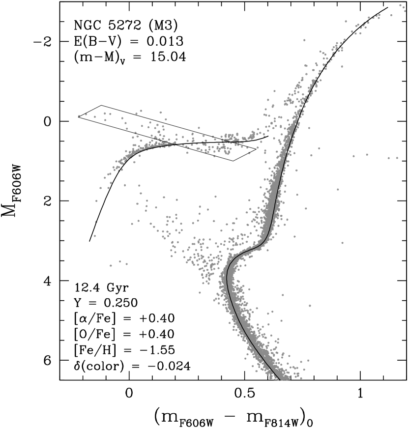
Figure 2.— Fit of a 12.4 Gyr isochrone for the indicated chemical abundances to the turnoff and subgiant photometry of M 3, assuming $E(B-V)=0.013$ and $(m-M)_{V}=15.04$, as found from the ZAHB models. The apparent distance modulus in the $F606W$ magnitude was calculated from the relation $(m-M)_{F606W}=(m-M)_{V}-0.246E(B-V)$; see CV14. (Note that RR Lyrae at different phases of their pulsation cycles are responsible for most of the scatter of points in the region contained within the parallelogram. Because the HST observations were taken as part of a snap-shot survey, magnitude- or intensity-weighted mean magnitudes cannot be calculated for the variable stars from those data.) To reproduce the TO color, the isochrone had to be adjusted by 0.024 mag to the blue.

As it is usually worthwhile to examine fits of isochrones to as many different CMDs as possible, we have opted to consider both the HST photometry of M 3 that was obtained by Sarajedini et al. (2007) and the latest calibration of ground-based $BVI_{C}$ data by P. Stetson (as described, and used, in the study by VandenBerg et al. 2015). A plot of the $F606W,F814W$ observations is shown in Figure 2, which illustrates that a ZAHB for the indicated chemical abundances provides quite a good match to the lower bound of the distribution of non-variable HB stars at $(m_{F606W}-m_{F814W})_{0}\mathrel{\hbox{\raise 2.58334pt\hbox{$<$}\kern-7.74998pt\lower 2.15277pt\hbox{$\sim$}}}0.2$ and $\mathrel{\hbox{\raise 2.58334pt\hbox{$>$}\kern-7.3194pt\lower 2.15277pt\hbox{$\sim$}}}0.4$. The isochrone, for the same abundances, that provides the best fit to the TO and SGB is one for an age of $\approx 12.4$ Gyr. While a small color offset had to be applied to the isochrone in order to match the observed turnoff color, this has no impact on the inferred age (see V13). It does indicate, however, that there must be a small problem with, e.g., the model ${T_{\rm eff}}$ scale, the adopted color transformations, the photometric zero-points, and/or the assumed chemical composition. Regardless, the level of agreement between theory and observations is quite satisfactory when the adopted or derived properties of M 3 are close to currently favored values (see, e.g., the entries for this GC in the latest edition of the catalog by Harris 1996, see our footnote 4).

The same can be said of Figure 3, which is identical to Fig. 2 except that the isochrones are compared with the principal photometric sequences of M 3 on the $[(V-I_{C})_{0},\,M_{V}]$-plane. Interestingly, the predicted and observed turnoff colors agree to within 0.002 mag, but the cluster RGB is offset to the blue by a larger amount than in the previous plot. Because of the many factors that play a role in such comparisons, it is not easy to determine which one is mostly responsible for these discrepancies. It seems unlikely that they can be attributed primarily to errors in the predicted temperatures because any ${T_{\rm eff}}$ adjustments that eliminate the problems in one CMD will exacerbate the difficulties in the other CMD — especially in view of the similarity between $(F606W,\,F814W)$ and Johnson-Cousins $(V,\,I_{C})$. Aside from small zero-point errors, the photometry is probably quite reliable in a systematic sense, but this may not be true of current color–${T_{\rm eff}}$ relations. In any case, it is very encouraging to find that the quality of the fits to both the HB and the TO observations are comparable in Figs. 2 and 3.

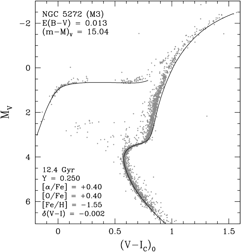
Figure 3.— Similar to the previous figure, except that the stellar models are compared with $VI_{C}$ observations of M 3.

Remarkably, of the three CMDs that have been considered, the same stellar models provide the best match to the $[(B-V)_{0},\,M_{V}]$-diagram of M 3, as shown in Figure 4. This is unexpected because the blanketing is more severe, and hence more problematic from the modeling perspective, in the $B$ bandpass than at longer wavelengths. Figs. 2–4 thus demonstrate that inconsistencies in predicted colors at the level of a few hundredths of a magnitude, especially for cool stars, are unavoidable. However, the ZAHB-based apparent distance moduli and predicted ages are largely independent of color-related uncertainties. It is worth mentioning that VandenBerg et al. (2015) used the same isochrones, but different ZAHB models, in their fits to the same $BV$ photometry of M 3. They obtained an age of 12.25 Gyr, which is slightly younger than our determination (12.4 Gyr), because they adopted a slightly larger value of $(m-M)_{V}$. An even younger age (11.75 Gyr) was derived by V13 in their survey of GC ages, due mainly to their use of stellar models that assumed a significantly higher abundance of oxygen, which more than compensated for a reduced distance modulus.

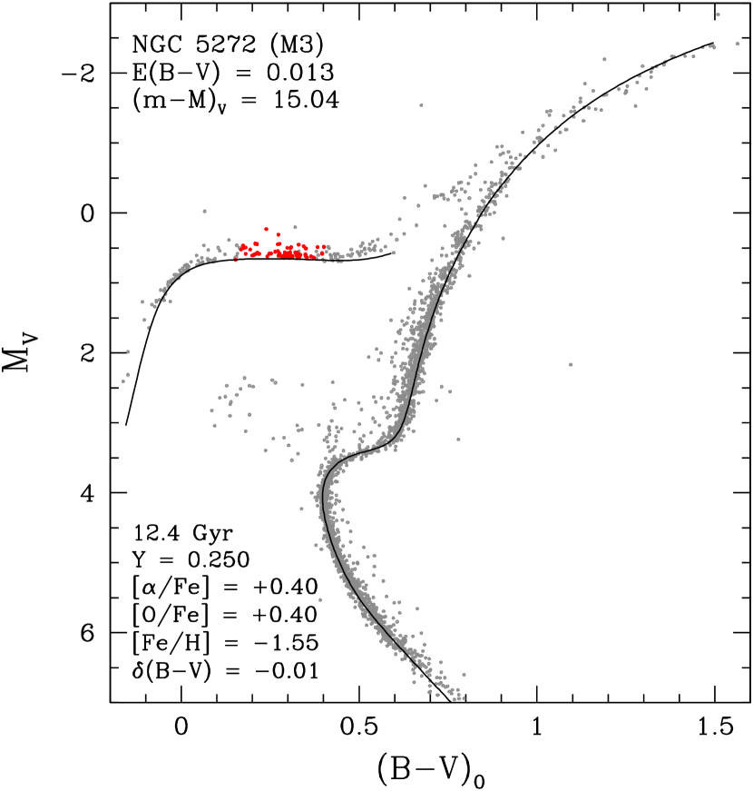
Figure 4.— Similar to the previous two figures, except that the stellar models are compared with $BV$ observations of M 3. The “static equivalent” properties of the sample of RR Lyrae stars that are considered in this paper (see the text) have been plotted as small red filled circles.

The RR Lyrae that appear in Fig. 4 as red dots were taken from the study by Cacciari et al. (2005, their Tables 1 and 2). All variables that were flagged as having large scatter in their light curves or low amplitudes (a possible sign of blends), or which exhibited some evidence for the presence of companions or for the Blazhko effect (see, e.g., Buchler & Kolláth 2011, and references therein), were removed from the sample. However, even when such strict selection criteria are adopted — which we can afford to employ in the case of such an RR Lyrae-rich cluster as M 3 — we are still left with a total sample of 69 variables, 46 of which are fundamental ($ab$-type) pulsators and 23 of which are first-overtone ($c$-type) pulsators.

Cacciari et al. (2005) converted colors (but not magnitudes) to their static equivalents, based on the prescriptions given by Bono et al. (1995). (Fortunately, the differences between the static colors so derived and magnitude-weighted mean colors are typically $\mathrel{\hbox{\raise 2.58334pt\hbox{$<$}\kern-7.74998pt\lower 2.15277pt\hbox{$\sim$}}}0.02$ mag.) By interpolating in the Bono et al. tables, we were able to compute the static $V$ magnitudes for the M 3 RR Lyrae. It turns out that they generally agree to within $\sim 0.002$ mag with the mean magnitudes given by Cacciari et al., who integrated the light curves in intensity and then converted the resultant integrations to magnitudes. Accordingly, we have simply adopted the values of $\langle V\rangle_{i}$ and $(B-V)_{S}$ that are tabulated by Cacciari et al.

Figure 5.— Overlay of evolutionary tracks for core He-burning stars and the same ZAHB that appears in the previous figure onto the CMD for the HB and RGB populations of M 3 that have $0.1\leq M_{V}\leq 1.4$. Filled and open circles (in red) identify the $ab$-type and $c$-type RR Lyrae, respectively.

Figure 5 focuses in on the region of the CMD that contains the RR Lyrae and non-variable HB stars of M 3, as well as cluster giants that lie within the same range of $M_{V}$. The stars and ZAHB that appeared in the previous figure are reproduced here, but different symbols are used to identify the fundamental and first-overtone pulsators (as noted). A grid of post-ZAHB tracks, for the same initial chemical abundances that were assumed in the isochrones (see Figs. 2–4) and for masses in the range of 0.80–0.58 ${\cal M_{\odot}}$ (in the direction from red to blue colors) has been superimposed on the observations. They begin at the ZAHB and end when the central helium abundance has fallen to $Y_{C}\sim 0.01$, which typically takes $\sim 90$ Myr.

Except for the four most massive HB models, evolutionary sequences were computed for masses that differed by $0.005{\cal M_{\odot}}$ in the vicinity of the instability strip, rising to $0.01{\cal M_{\odot}}$ for the hottest models. This spacing is sufficiently fine that precise predictions of the masses, luminosities, and effective temperatures of the RR Lyrae stars can be obtained simply by linear interpolations within the grid (or by extrapolating just outside of it, in the case of the brightest variables). Since the stellar models were computed for $Z=7.623\times 10^{-4}$, the periods of the variables can be calculated using equations (1) and (2), and then compared with the observed periods.

The results of this exercise are better than one might have expected (as we will show shortly), though the computed periods for the $ab$-type variables tend to be somewhat too low. The most likely explanations of this problem are (i) the predicted temperatures are too high — despite the fact that isochrones need to be shifted to the blue to match the turnoff color, which goes in the opposite direction, (ii) the values of $(B-V)_{S}$ given by Cacciari et al. (2005) are too blue, or (iii) the coefficient that multiplies $\log{T_{\rm eff}}$ should be reduced (in an absolute sense). It is well known that the temperatures of stellar models are much more uncertain than their luminosities, and ${T_{\rm eff}}$ uncertainties will obviously have a much bigger impact on the calculated periods of RR Lyrae than those associated with luminosities or masses.

Figure 6.— Comparison of the observed periods, in days, of the $ab$- and $c$-type RR Lyrae in M 3 with those derived from the evolutionary tracks shown in the previous figure (for $Y=0.25$, [Fe/H] $=-1.55$, and [$\alpha$/Fe] $=+0.40$). The observed periods have the mean values that are given in the top, left-hand corner of the plot. The same values of $\langle P_{ab}\rangle$ and $\langle P_{c}\rangle$ are obtained for the predicted periods if the temperatures of the variables are adjusted by the amounts specified in the lower right-hand corner (see the text). Cacciari et al. (2005) estimate the internal errors in their $(B-V)_{S}$ colors to be typically 0.02 mag, which translates to errors in $\log{T_{\rm eff}}$ and the predicted periods, in turn, of $\approx 0.007$ and $\sim 0.03$ d. The measured periods are known to better than $\pm 0.00001$ d. The differences between the predicted and the observed periods have a standard deviation $\sigma=0.024$ d and 0.021 d in the case of the $ab$- and $c$-type variables, respectively.

In fact, rather good consistency between the predicted and observed periods, and the corresponding value of $\langle P_{ab}\rangle$, can be obtained if $-3.425$ is adopted instead of $-3.430$ for the $\log{T_{\rm eff}}$ coefficient, which has a $1\sigma$ uncertainty of $\pm 0.01$ according to equation (1). However, the periods given by period–mean-density relations involve relatively small uncertainties. That is, changes to the various coefficients and the zero point in different versions of such equations tend to compensate for one another so as to yield nearly the same periods; for some discussion of this point, see Catelan (1993). As a result, it is unlikely that the ${T_{\rm eff}}$ coefficients can be altered in equations (1) and (2) without concomitant changes to other coefficients.

For this reason, it is preferable to correct the predicted ${T_{\rm eff}}$ scale when attempting to match the observed values of $\langle P_{ab}\rangle$ and $\langle P_{c}\rangle$. (Doing so serves to compensate for errors in the adopted values of $(B-V)_{S}$, the color–${T_{\rm eff}}$ relations that are used, and the temperatures of the stellar models.) In Figure 6, the observed periods of the selected M 3 RR Lyrae stars are compared with those computed using equations (1) and (2) after the temperatures derived for them via interpolations in the grid of HB tracks shown in Fig. 5 have been adjusted by the amounts specified in the lower right-hand corner. With these adjustments, the calculated values of $\langle P_{ab}\rangle$ and $\langle P_{c}\rangle$ reproduce the observed values (given in the upper left-hand corner of the plot) to three decimal places. This consistency was achieved simply by iterating on the relevant $\delta\log{T_{\rm eff}}$ values. Note that a temperature reduction that was applied to the fundamental-mode pulsators has the effect of increasing the calculated period of an RR Lyrae that has $P_{ab}=0.55$ d by $\approx 0.024$ d. (Changes to the temperatures, luminosities, or masses that are predicted for a given RR Lyrae will move the point representing that star vertically up or down in Fig. 6 at the observed value of $\log P$. For instance, the two $c$-type variables that lie above the dashed line with observed periods of $\sim 0.42$ d would shift onto that line if their values of $\log{T_{\rm eff}}$, $M_{\rm bol}$, or mass were increased by 0.009 dex, 0.093 mag, or $0.08\,{\cal M_{\odot}}$, respectively.)

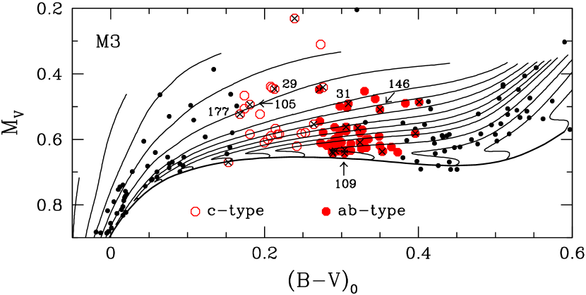
Figure 7.— A somewhat magnified version of Fig. 5 in which the RR Lyrae with $|\Delta P_{ab}|>0.024$ d and $|\Delta P_{c}|>0.021$  d are identified by crosses superimposed on the relevant open or filled circles. Variable identification numbers are specified only for those stars that are referenced explicitly in the text.

The dispersion in the predicted periods relative to the observed periods is presumably due mostly to errors in the values of $(B-V)_{S}$ that were determined by Cacciari et al. (2005), given that the HB evolutionary tracks are expected to be quite robust in a differential sense. Support for this assertion is provided in Figure 7, which shows a somewhat magnified version of Fig. 5 in which the stars with $|\Delta P_{ab}|>0.024$ d and $|\Delta P_{c}|>0.021$ d (i.e., the points furthest from the “line of equality” in Fig. 6) are identified by crosses. The majority of them are located in close proximity to stars for which the predicted and observed periods are in good agreement. This is certainly true of V109 and other crossed variables in the dense concentration of $ab$-type RR Lyrae at $M_{V}\sim 0.6$ and $(B-V)_{0}\sim 0.3$, but the same thing is found elsewhere in Fig. 7. For instance, the calculated periods of V105 and V177 differ, in turn, by $+0.022$ d and $-0.058$ d from their measured values, though the difference is only $+0.011$ d for the variable that is located between V105 and V177. Similarly, V29 and V31 have nearly the same CMD locations as other variables in which the predicted and observed periods agree to within $\pm 0.012$ d. In fact, consistency at this level is obtained for approximately half of the RR Lyrae stars in our sample. [Were we to drop from consideration the most discrepant points (i.e., the stars denoted by crosses in Fig. 7), the differences between the calculated and measured periods for the resultant sample of 32 $ab$-type and 16 $c$-type variables would have dispersions with $\sigma(\Delta P_{ab})=0.013$ d and $\sigma(\Delta P_{c})=0.009$ d.]

This is really very encouraging consistency between theory and observations given that such differences correspond to errors of $\mathrel{\hbox{\raise 2.58334pt\hbox{$<$}\kern-7.74998pt\lower 2.15277pt\hbox{$\sim$}}}\pm 0.004$ in the values of $\log{T_{\rm eff}}$ that are derived for the variables from the HB tracks and the adopted color–${T_{\rm eff}}$ relations (by CV14). The fact that the most problematic stars are roughly evenly distributed as functions of both magnitude and color, especially in the case of the fundamental-mode variables, suggests that the $\Delta P$ dispersions are primarily statistical fluctuations rather than, say, the consequence of chemical abundance variations (though the latter could be contributing factors). Note that the star with the largest difference between the predicted and observed period (0.080 d) is V146, which lies close to the middle of the color range spanned by the $ab$-type RR Lyrae.

Predicted luminosities also appear to be quite reliable. If $(m-M)_{V}=15.04$ is assumed for M 3 (see Figs. 2–4), $\langle M_{V}\rangle$ $=0.583$ is obtained for the entire sample of $ab$-type variables that we have considered. According to Clementini et al. (2003), the fundamental-mode pulsators residing in the Large Magellanic Cloud (LMC) have $\langle V_{0}\rangle=0.214($[Fe/H]$+1.5)+19.064$. On the assumption of the accurate eclipsing-binary distance derived by Pietrzyński et al. (2013) for the LMC, which corresponds to $(m-M)_{0}=18.494$, the Clementini et al. relation yields $\langle M_{V}\rangle$$=0.559$ for RR Lyrae that have [Fe/H] $=-1.55$ (the metallicity that we have adopted for M 3). This differs from our determination by only 0.024 mag, which is well within distance modulus and metallicity uncertainties (both for M 3 and the LMC variables). On the other hand, we could easily obtain a brighter value of $\langle M_{V}\rangle$ simply by adopting a slightly higher helium abundance or a lower [Fe/H] value. Indeed, a metallicity close to $-1.7$ (recall the work of Zinn & West 1984), or less, is well within the realm of possibility, especially as there has been some movement in recent spectroscopic investigations towards lower metallicities for metal-poor GCs (e.g., see Sobeck et al. 2011, Roederer & Sneden 2011, Roederer & Thompson 2015).

Although a reinvestigation of M 3 using the same methods and codes that were employed in the aforementioned studies has yet to be carried out, a lower [Fe/H] value would help to alleviate a possible problem with the interpretation of the M 3 HB shown in Figs. 5 and 7 by reducing the extent of the post-ZAHB blue loops. As discussed by Sandage (1981, see his Figs. 8, 9), one would expect to see some overlap of the colors of $ab$- and $c$-type variables, as a result of the hysteresis effect (van Albada & Baker 1973), if tracks with blue loops accurately describe the evolution of the observed HB stars. This is not a major problem for the models plotted in Figs. 5 and 7 because the lengths of the blue loops amount to no more than $\delta(B-V)\sim 0.05$ mag at the color which separates $c$- and $ab$-type variables, but the observations indicate that there is very little, if any, overlap whatsoever of the fundamental and first-overtone pulsators — at least for the sample of RR Lyrae that we have considered.

The limited work that we have done on this issue so far indicates that the lengths of blue loops, in the vicinity of the instability strip, decrease relatively slowly with [Fe/H]; i.e., they would still be present, but shortened by, e.g., $\sim 25$% at [Fe/H] $=-1.7$ (assuming constant $Y$ and [$\alpha$/Fe]). Higher helium abundances would exacerbate this problem (see below), but a small reduction in $Y$ and/or [CNO/Fe] (or an increased helium core mass; see Catelan 1992) would have beneficial consequences in this regard. It is worth mentioning that a modest decrease in the assumed [Fe/H] value produces no more than minor changes to the effective temperatures and masses that are derived from the corresponding HB models. Thus, we would have obtained a plot that is very similar to Fig. 6 had we adopted a lower [Fe/H] value for M 3 by, e.g., $\sim 0.15$ dex (while retaining the same values of the other chemical abundance parameters).

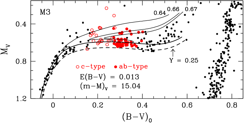
Figure 8.— Similar to Fig. 5, except that a ZAHB for $Y=0.27$ and associated evolutionary tracks for 0.64, 0.66, and 0.67 ${\cal M_{\odot}}$ have been superimposed onto the observed HB stars in M 3. The location of the same ZAHB (for $Y=0.25$) that appears in Fig. 5 is reproduced here as the dashed curve. Note that exactly the same reddening and distance modulus have been assumed in both figures.

The close matches of a ZAHB for constant $Y$ to the faintest HB stars over the entire ranges in color plotted in Figs. 2–5 provide a strong argument that at least the lowest luminosity HB stars in M 3 have nearly the same helium abundance. (The same conclusion was reached, based on similar findings, by Catelan et al. 2009, also see .) That our computations preclude variations of $Y$ by more than $\sim 0.005$ in these stars is demonstrated in Figure 8, which shows that the displacement at any color between the faintest HB stars and the ZAHB for $Y=0.25$ is a small fraction of the separation between ZAHBs for $Y=0.25$ and 0.27.

These results argue against the explanation of the Oosterhoff dichotomy recently proposed by Jang et al. (2014). In their scenario, the RR Lyrae in M 3 are expected to have lower helium abundances than the non-variable stars on either the red or blue sides of the instability strip, which should cause the latter to be somewhat brighter than the ZAHB that is relevant for the variable stars. (If anything, the faintest RR Lyrae appear to be slightly brighter than the non-variable stars to the left or right of them, but this could be the result of small zero-point differences in the photometry for the variable and non-variable stars, which come from different sources.)

However, Fig. 8 does not rule out the possibility that some fraction of the stars lying above the $Y=0.25$ ZAHB have higher helium abundances, including some of the brightest $c$-type variables, judging from their locations relative to the track for $Y=0.27$ and ${\cal M}=0.64\,{\cal M_{\odot}}$. [Unfortunately, it is not possible to use the predicted periods to constrain the helium abundances of the RR Lyrae because the only quantity that varies appreciably with $Y$ at a given CMD location, assuming fixed values of the reddening and distance modulus, is the mass, and its variation ($\sim 0.01$–0.03 ${\cal M_{\odot}}$ for $\delta Y\mathrel{\hbox{\raise 2.58334pt\hbox{$<$}\kern-7.74998pt\lower 2.15277pt\hbox{$\sim$}}}0.02$) has only a small effect on the period; see equations (1) and (2).]

As mentioned above, the apparent lack of any overlap of the colors of the $ab$- and $c$-type variables implies that stars which began their core He-burning lifetimes as fundamental-mode pulsators do not follow tracks that have blue loops or the blue loops are too small to reach very far into the region of the instability strip where only first-overtone pulsators are found (see Fig. 8 by Sandage 1981). Alternatively, the hysteresis mechanism does not occur in real stars. Since these loops are obviously quite a strong function of $Y$ (compare Figs. 7 and 8), a helium abundance slightly less than $Y=0.25$ (but within the uncertainties of the primordial helium abundance; see Komatsu et al. 2011) and/or some refinement of the assumed CNO content would appear to be necessary to explain the sharp boundary between the fundamental and first-overtone pulsators at $(B-V)_{0}\approx 0.27$. (Some additional discussion of this point is given in § 4.) In any case, our analysis suggests that most of the stars in M 3 have nearly the same helium abundance, though star-to-star variations as large as $\delta Y\sim 0.02$ cannot be ruled out.

As already mentioned, further constraints on the properties of M 3 may be obtained from a consideration of synthetic HB populations, but we defer such work to the next paper in the current series, which will be devoted to a study of M 3 and M 13.

3.2. M 92

Although most investigations over the years have found that M 92 has [Fe/H] $\sim-2.3$ (e.g., Zinn & West 1984, Sneden et al. 2000, Behr 2003, Carretta et al. 2009a), lower values by 0.2–0.4 dex have been obtained in some spectroscopic studies (e.g., Peterson et al. 1990, King et al. 1998), including the recent one by Roederer & Sneden (2011). In view of this, we decided to fit stellar models for [Fe/H] $=-2.30$ and $-2.60$ to the CMD of M 92, and to the properties of its variable stars, in order to determine whether they indicate any preference for one of these metallicities over the other.

The best available photometry for the cluster RR Lyrae is given by Kopacki (2001), who derived intensity-weighted mean $\langle V\rangle_{i}$ brightnesses and magnitude-weighted $(V-I_{C})_{m}$ color indices, as calculated from the difference in the magnitude-weighted magnitudes $(V)_{m}$ and $(I_{C})_{m}$, for the variables. We have therefore used $[(V-I_{C})_{0},\,M_{V}]$-diagrams throughout our study of M 92. However, we did verify that the ZAHB and best-fit isochrone on this CMD provide equally good interpretations of HST $F606W,\,F814W$ and $B,\,V$ data for the TO and HB stars. [These plots have not been included here because they merely serve to confirm what has already been demonstrated in Figs. 2–4 for M 3; namely, that small CMD-dependent zero-point and systematic offsets between predicted and observed colors are commonly found — though they do not affect the derived distance modulus and age.]

M 92 is known to have 17 RR Lyrae (Kopacki 2001), but only 12 of them (8 $ab$-types and 4 $c$-types) have reliable measured magnitudes according to the online version of the Clement et al. (2001) catalog of variable stars in GCs. The properties of one of the remaining fundamental pulsators (specifically, V6) seem suspect as well because it has a relatively short period (0.600 d) despite being the most luminous RR Lyrae ($\langle V\rangle_{i}=14.96$) and having a color (and therefore ${T_{\rm eff}}$) that is very similar to those of the other $ab$-type variables. By comparison, V1 has $\langle V\rangle_{i}=15.02$ and a period of 0.703 d. Because an unreasonably large mass would have to be invoked in order to explain the period of V6 using equation (1) if the values of $\langle V\rangle_{i}$ and $(V-I_{C})_{m}$ given by Kopacki for this star are adopted, something is clearly awry. For this reason, V6 has been dropped from further consideration.

3.2.1 Isochrones, ZAHBs, and RR Lyrae

The bottom panel of Figure 9 shows that a ZAHB for [Fe/H] $=-2.30$, [$\alpha$/Fe] $=0.4$ (e.g., Carney 1996, Sneden et al. 2000), and $Y=0.250$ provides quite a good fit to M 92’s faintest, non-variable blue HB stars if $(m-M)_{V}=14.74$ and the foreground reddening is $E(B-V)=0.023$ mag. This value of $Y$ is within the uncertainties associated with current estimates of the primodial abundance of helium and the abundances that have been derived from helium lines in the spectra of HB stars in M 30 and NGC 6397 with ${T_{\rm eff}}\sim 10^{4}$ K (see Mucciarelli et al. 2014, as well as references therein). (M 92 and M 30 probably have the same helium abundance given that they have nearly identical CMDs and ages; see V13.) The turnoff luminosity is well matched by a 12.9 Gyr isochrone for the same chemical abundances once the predicted colors are adjusted by $-0.013$ mag in order to fit the observed TO color.

Figure 9.— Bottom panel: Overlay of an isochrone for the indicated age and chemical abundances onto the CMD of M 92 after the predicted colors have been adjusted by $-0.013$ mag (as noted). The adopted reddening and the apparent distance modulus that has been derived from a fully consistent ZAHB, which has been plotted without any adjustment to the predicted colors, is specified in the top left-hand corner. Member RR Lyrae are represented by small red dots. Top panel: Superposition of the same ZAHB that appears in the bottom panel, along with several evolutionary tracks for the core He-burning phase, onto the CMD for the HB and RGB populations of M 92 that have $0.1\leq M_{V}\leq 1.4$. Only those tracks for models with ${\cal M}\leq 0.71{\cal M_{\odot}}$ have been plotted. Filled and open circles (in red) identify the $ab$-type and $c$-type RR Lyrae stars, respectively.

The models faithfully reproduce the morphologies of the MS and RGB fiducial sequences, though the predicted giant-branch location is too red by a few hundredths of a magnitude. Errors associated with the adopted color–${T_{\rm eff}}$ relations, convection theory, the atmospheric boundary conditions, or the assumed cluster parameters are some of the plausible explanations for such discrepancies. Note that the photometry was taken from VandenBerg et al. (2015, see their § 2), who obtained a slightly older age for M 92 (13.0 Gyr), mainly because they adopted a lower [Fe/H] value by 0.1 dex. Victoria models that assume higher values of [O/H] predict younger ages (see, e.g., V13), which further highlights the sensitivity of absolute GC ages to the adopted chemical abundances.

The same ZAHB that appears in the bottom panel of Fig. 9 is reproduced in the top panel, where several tracks for the core He-burning phase are also plotted. These follow the evolution of stars that arrive on the HB with the same helium core mass — but different envelope, and hence total, masses — until the central He abundance has decreased to $Y_{C}\sim 0.01$. (Because the tracks for the more massive models follow nearly the same path towards the asymptotic giant branch, making it very difficult to distinguish between them, only those tracks for ${\cal M}\leq 0.71{\cal M_{\odot}}$, which are the most relevant ones for the interpretation of the cluster RR Lyrae, are shown.)

The locations of the $ab$- and $c$-type RR Lyrae correspond to the values of $\langle V\rangle_{i}$ and $(V-I_{C})_{m}$ that were derived by Kopacki (2001). Unfortunately, it is not possible to improve upon these estimates of their static equivalent colors because the necessary recipes are not available: those given by Bono et al. (1995), which were used by Cacciari et al. (2005) for M 3 variables, are restricted to the $B$, $V$, and $K$ bands only. Based on the differences between the values of $(B-V)_{m}$ and $(B-V)_{S}$ that are tabulated by Cacciari et al., one might expect that $(V-I_{C})_{m}$ colors should be corrected by about $-0.01$ mag in order to better represent the colors of static stars. Anyway, Fig. 9 shows that there is no color overlap of the fundamental and first-overtone pulsators in M 92. In addition, it is apparent that the variables are all significantly more luminous than the ZAHB at their colors and, judging from the evolutionary sequences, they originate from ZAHB locations at $(V-I_{C})_{0}\mathrel{\hbox{\raise 2.58334pt\hbox{$<$}\kern-7.74998pt\lower 2.15277pt\hbox{$\sim$}}}0.1$, where the majority of the non-variable HB stars are located. Note that the reddest ZAHB model, at $(V-I)_{0}\approx 0.40$, is obtained if no mass loss occurs during the preceding evolution. To obtain redder ZAHB models with [Fe/H] $=-2.30$, it is necessary to increase the assumed oxygen abundance (see below).

Figure 10.— Similar to Fig. 6, except that the observed periods of the RR Lyrae in M 92 are compared with those calculated using equations (1) and (2) on the assumption of the luminosities, masses, and effective temperatures that are obtained by interpolating within the grids of HB tracks at the CMD locations of the cluster RR Lyrae stars (see the top panel in the previous figure). The $\delta\log{T_{\rm eff}}$ offsets specified in the lower right-hand corner of the plot were applied to the interpolated temperatures.

By interpolating within the grid of HB tracks, the values of $\log(L/L_{\odot})$, $\log({\cal M}/{\cal M}_{\odot})$, and $\log\,{T_{\rm eff}}$ for each variable can be derived, from which its period may be calculated using equation (1) or (2). (For the models that appear in Fig. 9, $Z=1.357\times 10^{-4}$.) As discussed in connection with Fig. 6, one can iterate on $\delta\log{T_{\rm eff}}$ adjustment that is applied to the interpolated temperatures of the variables until the computed values of $\langle P_{ab}\rangle$ and $\langle P_{c}\rangle$ agree with the observed values. The results obtained via this procedure are illustrated in Figure 10. The small dispersion in the points about the dashed line, especially for the $c$-type variables, indicates that the models do quite a good job of explaining the properties of the RR Lyrae that reside in M 92. [If the two most discrepant $ab$-type variables were removed from the sample, we would obtain $\sigma(\Delta P_{ab})=0.010$ d. These stars are the bluest and the reddest filled circles in the upper panel of Fig. 9 at $M_{V}\sim 0.38$.]

In fact, this conclusion is not strongly dependent on the assumption that the colors of equivalent static stars correspond exactly to $(V-I_{C})_{m}$. If these colors are adjusted by, e.g., $-0.01$ mag, one obtains a virtually identical plot to that shown in Fig. 10 if the temperatures of the $ab$- and $c$-type variables are adjusted by $\delta\log{T_{\rm eff}}=-0.0071$ and $+0.0013$, respectively. These differences are still comparable to, or smaller than the $1\sigma$ uncertainty in the model ${T_{\rm eff}}$ scale. [In making this assertion, we are assuming that our models predict the temperatures of HB stars just as well as in the case of turnoff stars at similar metallicities and ${T_{\rm eff}}$ values. For a discussion of the uncertainties in the temperatures of main-sequence stars that are derived using the Infrared Flux Method (IRFM), reference may be made to Casagrande et al. (2010). The success of modern isochrones in matching the IRFM results to well within their uncertainties is demonstrated by VandenBerg et al. (2010).]

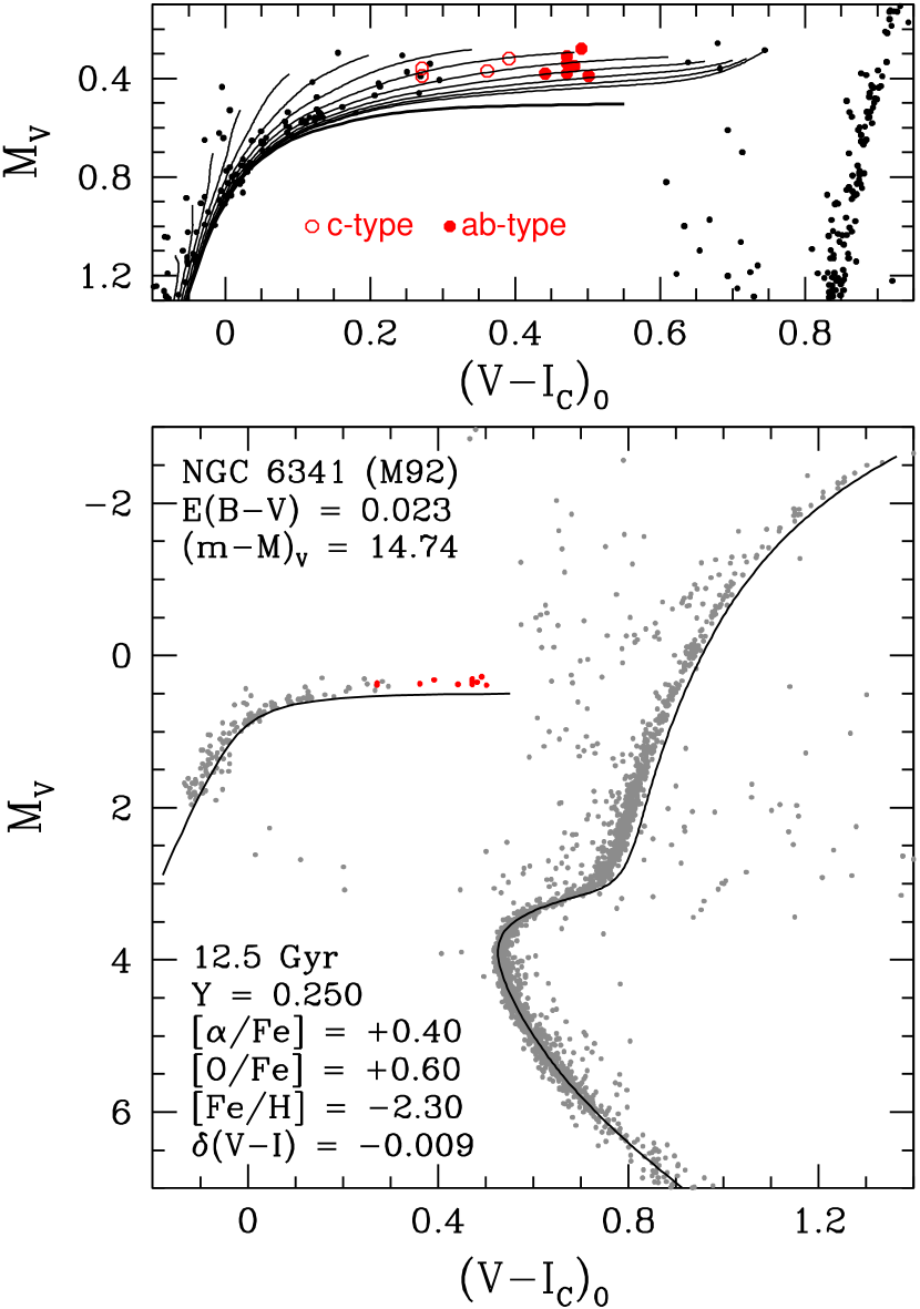
Figure 11.— As in Fig. 9, except that the stellar models assume [O/Fe] $=0.6$.

A plot that is indistinguishable from Fig. 10 is also obtained if models for a higher oxygen abundance by 0.2 dex (resulting in $Z=1.786\times 10^{-4}$) are fitted to the observations (see Figure 11), provided that $-0.0021$ and $+0.0053$ are adopted, in turn, for the $\delta\log{T_{\rm eff}}$ adjustments to the temperatures predicted for the fundamental and first-overtone pulsators. Higher oxygen stretches metal-poor ZAHBs to redder colors and, at their red ends, to slightly fainter $V$-band magnitudes (compare the ZAHBs for [O/Fe] $=0.4$ and 0.6 in the upper panels of Figs. 9 and 11, respectively). Both sets of models assume the same abundances of helium and the other metals. The main difference between the tracks that pass through, or close to, the RR Lyrae in these plots is a change in the predicted mass by $\approx 0.01\,{\cal M_{\odot}}$. For instance, the track that intersects the reddest open circle in Fig. 9 was computed for a $0.670\,{\cal M_{\odot}}$ model, whereas the corresponding track in Fig. 11 assumed a mass of $0.660\,{\cal M_{\odot}}$. The difference in mass is too small to have important consequences for the predicted periods; as a result, Fig. 10 is relatively insensitive to modest variations in [O/Fe].

Because the computed ZAHBs for [O/Fe] $=0.4$ and $0.6$ are nearly coincident at $(V-I_{C})_{0}\mathrel{\hbox{\raise 2.58334pt\hbox{$<$}\kern-7.74998pt\lower 2.15277pt\hbox{$\sim$}}}0.05$, where the majority of the “zero-age” HB stars in M 92 appear to be located, essentially the same value of $(m-M)_{V}$ is implied by both sequences. However, turnoff luminosity versus age relations depend quite strongly on the absolute abundance of oxygen (see, e.g., VandenBerg et al. 2014b, their Fig. 2), or more generally [CNO/H] (assuming fixed solar abundances of CNO). Hence, as shown in the bottom panel of Fig. 11, the inferred age of M 92 is reduced by about 0.4 Gyr to 12.5 Gyr, if [O/Fe] $=0.6$, as compared with $\approx 12.9$ Gyr in Fig. 9, if the cluster stars have [O/Fe] $=0.4$.

A virtually identical fit to the MS, TO, and RGB populations of M 92 can be obtained from isochrones for [Fe/H] $=-2.60$ and the same helium abundance and metals mixture that are specified in Fig. 11 on the assumption of $E(B-V)=0.023$ and $(m-M)_{V}=14.78$ (as found from a fully consistent ZAHB). The net effect of assuming a lower value of [O/H] by 0.3 dex and a larger distance modulus by 0.04 mag is to increase the predicted age to $\approx 12.8$ Gyr. It turns out that the isochrone for this age reproduces the turnoff color without requiring any adjustment of the predicted colors. Aside from these differences, it is not possible to distinguish between the fits of the [Fe/H] $=-2.60$ and $-2.30$ isochrones to the turnoff and giant-branch photometry. Accordingly, we have chosen to present the equivalent of just the top panel in Fig. 11; i.e., a plot in which the ZAHB and selected HB tracks for [Fe/H] $=-2.60$ and [O/Fe] $=0.6$ have been fitted to the cluster HB population.

As shown in Figure 12, the reddest ZAHB model has $(V-I_{C})_{0}\approx 0.25$, which is considerably bluer than those plotted in Figs. 9 and 11 due to the combined effects of lower [Fe/H] and (especially) reduced [O/H]. Nevertheless, the superposition of the HB tracks onto the variable stars closely resembles those shown previously. In fact, the interpolated luminosities, effective temperatures, and masses at the CMD locations of the RR Lyrae are all sufficiently similar to those derived from the models for [Fe/H] $=-2.30$ that the periods calculated for them using equations (1) and (2), assuming the appropriate value of $Z$ ($8.951\times 10^{-5}$), are not very different either.

To be more specific: the adoption of a larger distance modulus by 0.04 mag implies higher luminosities by $\delta\log(L/L_{\odot})\approx 0.016$ and higher periods for the $ab$-type RR Lyrae by $\delta\log P_{ab}\approx 0.014$ (see equation 1). However, the predicted mass of each variable increases by $\approx 0.015{\cal M_{\odot}}$ and the resultant changes to $\log\,P_{ab}$ given by the $\log({\cal M}/{\cal M_{\odot}})$ and $\log\,Z$ terms in equation (1) amount to $\approx-0.014$, with some minor star-to-star variations of these numbers. (Basically the same thing is found for the $c$-type variables. Note that the predicted temperatures at a given $V-I_{C}$ color do not change significantly if the [Fe/H] value is reduced from $-2.30$ to $-2.60$.) As a result, the comparison between the predicted and observed periods can hardly be distinguished from that shown in Fig. 10 if the inferred temperatures of the $ab$- and $c$-type pulsators are adjusted by $\delta\log{T_{\rm eff}}=-0.0021$ and $+0.0063$, respectively. As before, these choices are set by the requirement that the models for [Fe/H] $=-2.60$ and [O/Fe] $=0.6$ predict the observed values of $\langle P_{ab}\rangle$ and $\langle P_{c}\rangle$. Thus, Fig. 10 is obtained for M 92 largely independently of moderate variations in the adopted values of [Fe/H] and [O/Fe].

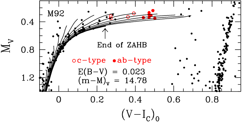
Figure 12.— Similar to the upper panel in the previous figure, except that the ZAHB and evolutionary tracks (for ${\cal M}\leq 0.72{\cal M_{\odot}}$) that are compared with the observations of M 92 assume [Fe/H] $=-2.60$.

Although it is disappointing that the predicted periods of the RR Lyrae do not provide a good constraint on the cluster metallicity, in view of the uncertainties associated with the former, it is nonetheless encouraging that up-to-date HB models provide a satisfactory explanation of the properties of the variable stars in both M 92 and M 3. This includes, in particular, the differences in $\langle P_{ab}\rangle$ and $\langle P_{c}\rangle$ between them. In addition, our findings support the canonical understanding of the HB phase of evolution, given that the faintest “zero-age” cluster stars are matched exceedingly well by a ZAHB for constant $Y$ over the entire range in color spanned by them. Neither the fits of ZAHB models to the cluster counterparts nor the comparisons between predicted and observed RR Lyrae periods provide any compelling evidence for large star-to-star helium abundance variations. While the methods that we have employed cannot detect the presence of modest variations (at the level of, say, $\delta Y\mathrel{\hbox{\raise 2.58334pt\hbox{$<$}\kern-7.74998pt\lower 2.15277pt\hbox{$\sim$}}}0.02$), any stars with $Y\mathrel{\hbox{\raise 2.58334pt\hbox{$>$}\kern-7.3194pt\lower 2.15277pt\hbox{$\sim$}}}0.27$ that reside in M 3 and/or M 92 must lie within the blue tails of their respective HB populations.

One of the conclusions that can be drawn from the work described above is that the distance moduli of M 3 and M 92 must be reasonably close to the values implied by ZAHB models for $Y=0.25$ and [Fe/H] values in the range of roughly $-2.3$ to $-2.6$, as found spectroscopically. (As shown in Figs. 9 and 11, distances derived in this way are virtually independent of [O/Fe], which mainly affects the predicted temperatures and colors of the more massive ZAHB models. [Fe/H] uncertainties also have relatively minor ramifications for ZAHB-based distance moduli given that $M_{V}$(HB) $\propto 0.21$ [Fe/H] in the vicinity of the instability strip; see V13, Clementini et al. 2003.) Although our determination of $(m-M)_{V}=15.04$ for M 3 agrees well with many estimates (e.g., 15.07 is listed in the Harris catalog; see our footnote 4), the distance modulus of M 92 is more controversial. Some discussion of this issue and of the implications of our derived value of $(m-M)_{V}=14.74$ for M 92 is warranted before we turn our attention to M 15.

3.2.2 The distance modulus of M 92

Relatively short distance moduli have generally been derived for M 92 when nearby field halo subgiants, of which HD 140283 is the most famous example, are used as standard candles (e.g., Pont et al. 1998, VandenBerg et al. 2002). Such stars, which can be age-dated directly because they are located in the region of a CMD where isochrones are most widely separated, are undeniably very old. The strongest evidence that they must have formed very soon after the Big Bang is provided by the work of VandenBerg et al. (2014b, also see ), who derived an age of $14.3\pm 0.8$ Gyr for HD 140283 (where the stated uncertainty takes into account all sources of error, including the parallax) using diffusive Victoria models that were computed for metal abundances derived from high-resolution, high S/N spectra..

A few comments are in order concerning the latest study of HD 140283 by Creevey et al. (2015), who found an age of $13.7\pm 0.7$ Gyr (or less, if its reddening is non-zero). The somewhat younger age that they determined may be due, in part, to their use of stellar evolutionary computations that, unlike those employed by VandenBerg et al. (2014b), apparently did not take into account the important revisions to the rate of the ¹⁴N$(p,\,\gamma)^{15}$O reaction that occurred about a decade ago (Formicola et al. 2004, also see ). In addition, the low ${T_{\rm eff}}$ that Creevey et al. derived for HD 140283 can be reproduced by stellar models only if very small values for the mixing-length parameter ($\mathrel{\hbox{\raise 2.58334pt\hbox{$<$}\kern-7.74998pt\lower 2.15277pt\hbox{$\sim$}}}1.0$) are assumed. Such low values of $\alpha_{\rm MLT}$ have never been found in studies of star cluster CMDs (see, e.g., VandenBerg et al. 2000, Salaris et al. 2002), which provide far better constraints on the value of this parameter than the properties of single stars (aside from the Sun) because the location and slope of the giant branch, as well as the length of the SGB, are very sensitive to the treatment of convection (see, e.g., VandenBerg 1983). These features cannot be reproduced unless a high value of $\alpha_{\rm MLT}$ is assumed (see Figs. 2–4, 9, and 11 in the present paper). In fact, 3D hydrodynamical model atmospheres do not favor low values of $\alpha_{\rm MLT}$ either (Magic et al. 2015).

Even though the solar-calibrated value of $\alpha_{\rm MLT}$ can vary significantly from one study to the next, due to different assumptions concerning e.g., the adopted solar abundances and the treatment of the surface boundary conditions, isochrones for this value of the mixing-length parameter generally provide credible fits to the CMDs of clusters for any metallicity. This can be seen by inspecting the plots provided by Dotter et al. (2008), Dell’Omodarme et al. (2012), and V14, whose models were computed on the assumption of solar-calibrated values of $\alpha_{\rm MLT}=1.938$, 1.74, and 2.007, respectively. The uncertainties of the various factors that play a role in comparisons of isochrones with observed CMDs are such that small variations in the mixing-length parameter with mass, chemical abundances, or evolutionary state cannot be ruled out, but neither has it been possible to argue compellingly in support of such variations (also see Ferraro et al. 2006). Granted, there are indications from 3D model atmospheres that $\alpha_{\rm MLT}$ should vary with ${T_{\rm eff}}$, gravity, and metallicity (e.g., Trampedach & Stein 2011; Magic et al. 2013, 2015), but the first attempts to implement the predictions from such simulations into stellar models have found that the resultant tracks are not very different from those that assume constant $\alpha_{\rm MLT}$ (Salaris & Cassisi 2015).

Creevey et al. (2015) have commented that the oxygen abundance that was derived by VandenBerg et al. (2014b) is based on a higher ${T_{\rm eff}}$ than their determination. However, that abundance, [O/Fe] $=0.64$, agrees very well with the trends between [O/Fe] and [Fe/H] given by Dobrovolskas et al. (2015) and Amarsi et al. (2015) for field Population II stars that have [Fe/H] $<-2.0$. To reduce the predicted age of HD 140283, an even higher O abundance would be required, which would suggest that the ${T_{\rm eff}}$ value adopted by VandenBerg et al. should be increased. That is, a cooler ${T_{\rm eff}}$ and the consequent decrease in [O/H] that would be needed to explain the observed line strengths would tend to increase the discrepancy between the age of the field subgiant and the age of the universe. It is also worth pointing out that a hot ${T_{\rm eff}}$ scale is supported by the recent calibration of the Infrared Flux Method by Casagrande et al. (2010), the color-temperature relations implied by MARCS model atmospheres (see CV14), and comparisons of stellar models with the properties of solar neighborhood subdwarfs with well-determined distances (VandenBerg et al. 2010, 2014a; Brasseur et al. 2010). The spectroscopically derived temperature of HD 140283 reported by VandenBerg et al. (2014b) is consistent with these photometric and theoretical determinations, but not the one obtained by Creevey et al. Further work is clearly needed to resolve this controversy; in particular, a further examination of the model-dependent aspects of the analysis of interferometric and spectroscopic data carried out by Creevey et al. may shed some light on this difficulty.

Returning to the matter at hand: since metal-poor GCs are generally thought to be among the oldest objects in the universe, one would expect that M 92 and HD 140283, which appear to have very similar metallicities, would be nearly coeval. In this case, cluster subgiants with the same intrinsic color as HD 140283 should have the same absolute $V$-magnitude. As shown in Figure 13, this would imply that M 92 has $(m-M)_{V}=14.54$, which causes the cluster HB stars to be fainter than ZAHB models for $Y=0.25$, [Fe/H] $=-2.3$, [$\alpha$/Fe] $=0.4$, and [O/Fe] $=0.6$. (These abundances are close to those derived spectroscopically for HD 140283; see VandenBerg et al. 2014b.) This is less than the ZAHB-based distance modulus (see Fig. 11) by 0.20 mag.

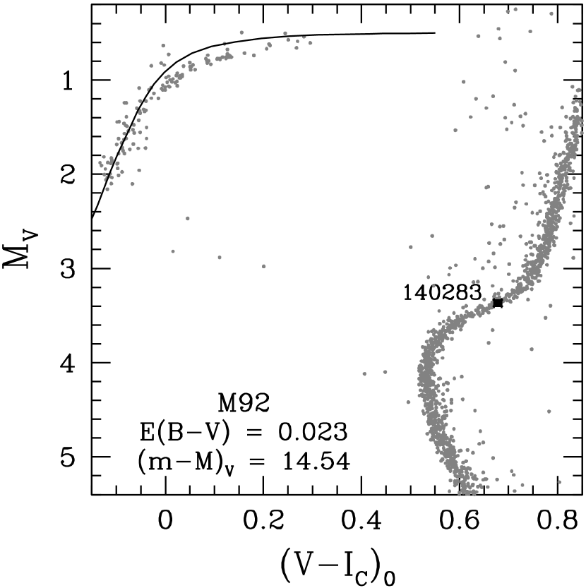
Figure 13.— Determination of the apparent distance modulus of M 92 if its SGB is matched to the CMD location of the field subgiant HD 140283. This assumes that both objects are chemically indistinguishable and that they have the same age, but it leads to irreconcilable differences between the ZAHB models for [Fe/H] $=-2.30$ and the observed HB of M 92.

However, we have already demonstrated that HB tracks for [Fe/H] $=-2.30$ are able to explain the periods of the RR Lyrae in M 92 quite well if the cluster has $(m-M)_{V}=14.74$ (see Fig. 9). This would not be possible if the short distance modulus is assumed. If the same tracks that are plotted in the top panel of Fig. 11 were displaced to fainter magnitudes by 0.20 mag, which corresponds to $\delta\log(L/L_{\odot})\approx-0.08$, the predicted values of $\langle P_{ab}\rangle$ and $\langle P_{c}\rangle$ would decrease by $>0.062$ d according to equations (1) and (2). (The only way of explaining such a large offset is by assuming a helium abundance that is much smaller than the primordial value of $Y$, which is not justifiable.) This provides a strong argument against such a faint HB, and we therefore conclude that M 92 subgiants of the same $(V-I_{C})_{0}$ color as HD 140283 must be intrinsically brighter than the field subgiant. If they are coeval and they have similar [Fe/H] values, M 92 must have lower [CNO/H] by $\mathrel{\hbox{\raise 2.58334pt\hbox{$>$}\kern-7.3194pt\lower 2.15277pt\hbox{$\sim$}}}0.5$ dex — but this is not supported by current spectroscopy; e.g., see Sneden et al. (2000). The most likely explanation is that M 92 is younger than HD 140283 (by up to $\sim 1$ Gyr, depending primarily on the difference in their respective CNO abundances).

Curiously, field Pop. II subdwarfs seem to favor a larger distance modulus for M 92 than HD 140283. Chaboyer et al. (2013) have reported preliminary results for three stars for which they obtained improved parallaxes using the HST Fine Guidance Sensors. Only one of them has [Fe/H] $<-2.0$; namely, HD 106924, which has [Fe/H] $=-2.13$, [O/Fe] $=0.60$, $M_{F606W}=5.96$ (with an uncertainty of about $\pm 0.015$ mag), and $m_{F606W}-m_{F814W}\approx 0.601$. (These photometric properties were obtained by interpolating in their Fig. 1.) As shown in Figure 14, there is very little separation between isochrones for [Fe/H] $=-2.0$ and $-2.6$ at the location of HD 106924 on the $[(m_{F606W}-m_{F814W})_{0},\,M_{F606W}]$-diagram. As a result, uncertainties in the measured metallicity of the subdwarf should have no more than relatively minor consequences. (We note, however, that Chaboyer et al. adopted a significantly cooler ${T_{\rm eff}}$ for it than that implied by the MARCS color transformations, so a metallicity $>-2.0$ cannot be entirely ruled out.)

Figure 14.— Comparison of the location of the field subdwarf HD 106924 (large red open circle) with the CMD of M 92 on the assumption of the indicated reddening and ZAHB-based distance modulus. The solid and dashed curves represent, in turn, isochrones for [Fe/H] $=-2.6$ and $-2.0$ for the specified values of age, $Y$, [$\alpha$/Fe], and [O/Fe]. The isochrones were adjusted to the blue by 0.007 mag.

If M 92 is assumed to have [Fe/H] $=-2.6$ (Roederer & Sneden 2011) and the other chemical abundance parameters have the indicated values, the ZAHB-based distance modulus is $(m-M)_{V}=14.78$ if $E(B-V)=0.023$. When these values are adopted, HD 106924 lies just to the red of the mean fiducial sequence of M 92 at the observed subdwarf magnitude — or, alternatively, HD 106924 is slightly brighter than cluster main-sequence stars that have the same color. A better centering of HD 106924 onto the CMD of M 92 would be obtained if $(m-M)_{V}\approx 14.84$. The uncertainties associated with the reddening and the fit of the ZAHB to the cluster HB population certainly permit a larger distance modulus by a few hundredths of a magnitude. It is also possible that the slight color offset of HD 106924 relative to the M 92 main sequence is due to small zero-point differences in the photometry of the two objects.

Another way of eliminating the apparent discrepancy is to adopt a higher He abundance by $\delta Y\sim 0.015$, which implies a brighter HB, and thereby an increased ZAHB-based distance modulus, by about 0.06 mag (or $\delta\log(L/L_{\odot})\approx 0.024)$. We have checked that a ZAHB for $Y=0.265$ provides an equally good fit to the lower bound of the distribution of HB stars in M 92 as one for $Y=0.25$ (see Figs. 9–12) when the aforementioned adjustment to the value of $(m-M)_{V}$ is adopted. That is, such a small change in $Y$ does not have detectable consequences for the quality of the model fits to the observed CMD (including fits of isochrones to the turnoff photometry).

On the other hand, making the RR Lyrae stars brighter through the adoption of a larger distance modulus would increase the predicted periods of the variables; see equations (1) and (2). However, the temperature uncertainties are large enough that one could recover the results shown in Fig. 10, on the assumption of $Y=0.265$ instead of $Y=0.25$, if higher temperatures by only $\delta\log{T_{\rm eff}}\sim 0.006$ were adopted. Since this is within the $1\sigma$ error bar of the model ${T_{\rm eff}}$ scale, we conclude that RR Lyrae periods alone cannot be used to provide a compelling argument in support of a particular He abundance within the range $0.25\mathrel{\hbox{\raise 2.58334pt\hbox{$<$}\kern-7.74998pt\lower 2.15277pt\hbox{$\sim$}}}Y\mathrel{\hbox{\raise 2.58334pt\hbox{$<$}\kern-7.74998pt\lower 2.15277pt\hbox{$\sim$}}}0.265$. Accurate distances based on, e.g., the best available calibration of the RR Lyrae standard candle, which agree well with ZAHB-based distance determinations (as described in § 3.1), are needed to constrain the luminosities of such variables.

The main conclusion to be drawn from Fig. 14 is that there is reasonably good consistency between the distance modulus based on HD 106924 and that derived from ZAHB models. In fact, this was the reason why we opted to use the computations for [Fe/H] $=-2.6$ in this comparison instead of those for [Fe/H] $=-2.3$, since a higher metallicity implies a smaller ZAHB-based distance modulus by $\approx 0.04$ mag (see Figs. 9, 11). However, this is admittedly a weak argument in support of the possibility that M 92 has [Fe/H] $\mathrel{\hbox{\raise 2.58334pt\hbox{$<$}\kern-7.74998pt\lower 2.15277pt\hbox{$\sim$}}}-2.6$ and [O/Fe] $=+0.6$. A potential difficulty with these abundances is that, if M 92 and M 15 have very similar chemical compositions, as is generally believed to be the case, the ZAHB plotted in Fig. 14 is too blue to explain the large number of RR Lyrae in M 15 (recall our discussion in § 1). In order for that ZAHB to pass through the instability strip (as in the case of a ZAHB for [Fe/H] $=-2.3$ and [O/Fe] $=+0.6$; see Fig. 11), a higher oxygen abundance by $\mathrel{\hbox{\raise 2.58334pt\hbox{$>$}\kern-7.3194pt\lower 2.15277pt\hbox{$\sim$}}}0.3$ dex would be needed, thereby resulting in [O/H] $\sim-1.7$ for both [Fe/H] values.

3.3. M 15

As in the case of M 92, most spectroscopic studies have found [Fe/H] $\approx-2.3$ for M 15 (Sneden et al. 2000, Kraft & Ivans 2003, Cohen et al. 2005, Carretta et al. 2009a), but some of the same investigators now appear to favor values $\mathrel{\hbox{\raise 2.58334pt\hbox{$<$}\kern-7.74998pt\lower 2.15277pt\hbox{$\sim$}}}-2.6$ (Preston et al. 2006, Sobeck et al. 2011). Because ZAHBs and core He-burning tracks are much more dependent on [O/H] (and $Y$) than [Fe/H], a 0.3 dex reduction in the metallicity is not expected to have major consequences for the interpretation of the M 15 CMD provided that this change is accompanied by a 0.3 dex increase in [O/Fe] (as obtained if the [O/H] value is unchanged). This may, in fact, be problematic for M 15 since, as shown below, it appears to be necessary to adopt [O/Fe] $\mathrel{\hbox{\raise 2.58334pt\hbox{$>$}\kern-7.3194pt\lower 2.15277pt\hbox{$\sim$}}}0.8$, if [Fe/H] $=-2.3$ to explain its RR Lyrae stars. (Note that [O/Fe] values closer to $+0.3$ were typically derived in spectroscopic studies of this GC in the 1990s; see, e.g., Sneden et al. 1997.) Consequently, models for [Fe/H] $=-2.6$ would yield a similar interpretation of the data only if [O/Fe] $\mathrel{\hbox{\raise 2.58334pt\hbox{$>$}\kern-7.3194pt\lower 2.15277pt\hbox{$\sim$}}}1.1$. Because this seems uncomfortably high (e.g., field stars of the same [Fe/H] typically have [O/Fe] $\sim 0.75$; e.g., Dobrovolskas et al. 2015), we have decided to restrict the present analysis to models for [Fe/H] $=-2.3$. ([O/Fe] $\approx 0.8$ at [Fe/H] $=-2.3$ is also on the high side, but [N/Fe] $\sim 1.6$ in some M 15 giants (see Cohen et al. 2005) implies an initial O abundance corresponding to [O/Fe] $\sim 0.8$ if C$+$N$+$O is conserved and the same giants still have [O/Fe] $\sim 0.3$ and [C/Fe] $<-0.5$.)

Turning to the photometry of M 15: in their extensive study of the $F606W,\,F814W$ observations of 55 GCs from the Sarajedini et al. (2007) survey, V13 found that Victoria-Regina isochrones generally had to be shifted to the blue by 0.01–0.025 mag to match the observed turnoff color when reddenings from Schlegel et al. (1998), metallicities from Carretta et al. (2009a), and ZAHB-based distance moduli were adopted. In the case of clusters with [Fe/H] $<-2.2$, M 15 was the sole exception to this “rule” in that the requisite blueward shift was 0.038 mag, as compared with, e.g., 0.018 mag for M 92 and 0.020 mag for M 30. According to Carretta et al., all three of these clusters have the same [Fe/H] to within 0.02 dex, and V13 found that they have the same age (12.75 Gyr). Why, then, does M 15 apparently have an intrinsically bluer turnoff than M 92 and M 30? [Interestingly, V13 (see their Fig. 14) found that NGC 2808 similarly stood out among GCs with $-1.0>$ [Fe/H] $\geq-1.5$, and they suggested that isochrones for $Y=0.25$ may require an unusually large blueward color correction to match its turnoff because the NGC 2808 appears to contain stars with a wide range in helium abundance (perhaps up to $Y=0.40$; see Piotto et al. 2007). Is it possible that helium abundance variations are significantly larger in M 15 than in other GCs of similar metallicity?]

To try to answer these questions, we will attempt to explain the properties of the RR Lyrae variables that have been identified in M 15 (though it is expected that the highest-$Y$ stars would have very blue ZAHB locations and thus may not produce RR Lyrae stars). However, let us first revisit the V13 analysis in the light of some improvements that can be made to the CMDs of M 15 and M 92 and the use of different ZAHB models and isochrones.

Especially well-defined CMDs can be obtained by (i) separating the MS and RGB stars in the Sarajedini et al. (2007) catalog from those that lie to the blue of the giant branch, (ii) sorting the two samples into 0.1 mag bins, and (iii) ranking the stars in each bin in terms of $\sigma_{*}$, where $\sigma_{*}$ is the smaller of the tabulated values of $\sigma_{F606W}$ and $\sigma_{(F606W-F814W)}$. If all stars with $\sigma_{*}>0.02$ mag are excluded and the remaining stars with the smallest photometric uncertainties, up to a maximum number of 75 from each bin, are plotted, we obtain the CMDs for M 15 and M 92 that are shown in Figure 15. The adopted selection procedure has maximized the number of HB stars while limiting the vast number of MS (and RGB) stars to those with the best photometry. It is quite obvious from Fig. 15 that the M 15 CMD is considerably broader than that of M 92 at any magnitude (which may be due in part to the effects of differential reddening; see Larsen et al. 2015.)

Figure 15.— Left-hand panel: As in the bottom panel of Fig. 11, except that the models for the indicated chemical abundances and age are compared with HST photometry of M 92 (Sarajedini et al. 2007) rather than ground-based $VI_{C}$ data. Right-hand panel: Fit of the same ZAHB and isochrone to HST photometry of M 15 (also from Sarajedini et al.). Stars lying below the flat part of the ZAHB and many of those above the densest concentration of HB stars are RR Lyrae variables that have been observed at random phases of their pulsation cycles. Note that a different color offset had to be applied to the isochrone to fit the turnoff colors of the two clusters (see the text for some discussion of this point).

If the ZAHB and best-fit isochrone that appear in the bottom panel of Fig. 11 are transformed to $F606W,\,F814W$ magnitudes and compared with M 92 photometry on the assumption of the same reddening and apparent distance modulus, we obtain the plot shown in the left-hand panel of Fig. 15. To within the fitting uncertainties, the same age ($\approx 12.5$ Gyr) is found on both color planes. The right-hand panel shows that the same ZAHB provides a very good fit to the HB population of M 15 if $E(B-V)\approx 0.100$, which agrees very well with recent determinations of line-of-sight reddenings from dust maps (Schlegel et al. 1998, Schlafly & Finkbeiner 2011), and $(m-M)_{V}=15.42$. Under these assumptions, the same age is found for M 15 as for M 92, though the best-fit isochrone must be shifted by 0.032 mag to the blue to match the observed turnoff color, as compared with 0.013 mag in the case of M 92.

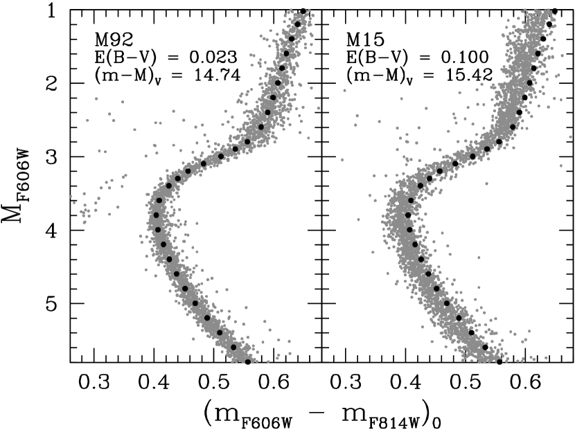
Figure 16.— Left-hand panel: Plot of the same M 92 photometry that appears in the previous figure for just the region of the CMD from the upper main sequence to the lower RGB, along with the mean fiducial sequence that has been derived from these stars (black filled circles). The adopted values of $E(B-V)$ and $(m-M)_{V}$ are the same as those indicated in Fig. 15. Right-hand panel: As in the left-hand panel, except that the median M 92 fiducial is superimposed on the M 15 CMD.

Figure 16 provides an alternative way of illustrating this difference. The left-hand panel reproduces the M 92 photometry from the previous figure for just the upper main sequence, subgiant, and lower RGB stars, on the assumption of exactly the same reddening and distance modulus. Using the methods described by V13 (see their § 5.3.1), the median locus through these stars was determined; this is the sequence consisting of black filled circles that has been superimposed on the smaller gray cluster stars. When compared with the M 15 observations from Fig 15 for $5.8\leq M_{F606W}\leq 1.0$ (see the right-hand panel), this sequence is obviously too red by about 0.02 mag to represent the M 15 CMD.

One might conclude from this intercomparison that the adopted reddening of M 15 is too high, since a much better superposition of the M 15 and M 92 turnoffs would be obtained if M 15 has $E(B-V)\approx 0.08$ rather than 0.10. However, as shown in Figure 17, such a low reddening presents problems for the interpretation of the bluest HB stars in this cluster, as most of them would then lie on the red side of the ZAHB at $M_{F606W}\mathrel{\hbox{\raise 2.58334pt\hbox{$>$}\kern-7.3194pt\lower 2.15277pt\hbox{$\sim$}}}1.8$. (According to canonical stellar evolutionary theory, the tracks of core He-burning stars always remain brighter than the associated ZAHB locus at a given color.) It would therefore appear to be the case that M 15 has an intrinsically bluer turnoff than M 92. (Differential reddening in M 15 could be partially responsible for the apparent offset in the turnoff colors, but it is unlikely to be the entire explanation; see below.)

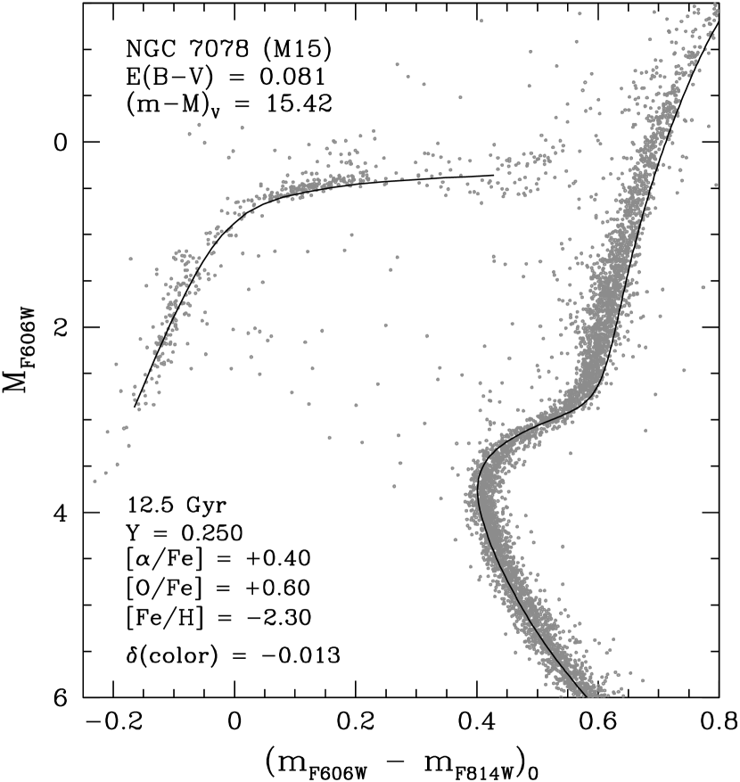
Figure 17.— As in the right-hand panel of Fig. 15, except that $E(B-V)=0.081$ has been assumed so that M 15 has the same intrinsic turnoff color as M 92. However, this leads to obvious problems with the fit of a ZAHB to the bluest HB stars.

A difference in [Fe/H] (for which there is little support, anyway) would have no more than a slight impact on the relative turnoff colors of M 92 and M 15 because the location of the MS on the [$(F606W-F814W)_{0},\,M_{F606W}$]-plane has almost no dependence on metallicity at [Fe/H] $\mathrel{\hbox{\raise 2.58334pt\hbox{$<$}\kern-7.74998pt\lower 2.15277pt\hbox{$\sim$}}}-2.3$ (as in the case of the similar [$(V-I_{C})_{0},\,M_{V}$]-diagram; see VandenBerg et al. 2010). Both clusters also seem to have quite similar abundances of most of the so-called $\alpha$-elements, such as Ca and Si (Sneden et al. 2000). We therefore suspect that helium abundance differences are responsible; in particular, that significantly larger variations in $Y$ are found in M 15 than in M 92. An examination of the properties of the RR Lyrae in M 15 should shed some light on this possiblity.

3.3.1 The RR Lyrae Stars in M 15

Even though the Clement et al. (2001) on-line catalog (see our footnote 9) has updated information on the variable stars in M 15 as recently as September 2014, it is acknowledged therein that the most modern study of the cluster RR Lyrae is still the one by Corwin et al. (2008). The main advance that has been made since then is some clarification of variable identifications. Using the astrometric catalogs given by Samus et al. (2009), Clement et al. found that a few of the new variables that Corwin et al. claim to have discovered were, in fact, previously known. Since we are using the Corwin et al. photometry (their Table 3) in the present study, we have ensured that such misidentifications do not affect the mean magnitudes and colors of the sample of variables that we have selected.

Stars for which the authors could not measure reliable $B$-, $V$-, or $I_{C}$-magnitudes were not considered, given the likelihood that the mean magnitudes for those stars would not be very trustworthy, along with a few stars that were either obviously too red (well outside the instability strip) or too faint (significantly fainter than ZAHB loci). Our final sample consists of 56 RR Lyrae (29 $ab$-type, 27 $c$-type) that are presumed to have reliable $B$ and $V$ measurements. Of these stars, 38 (23 $ab$-type, 15 $c$-type) appear to have reliable $V$ and $I_{C}$ magnitudes.

As in the case of M 3 and M 92, we checked that there is good consistency of the interpretations of the [$(B-V)_{0},\,M_{V}$]- and [$(V-I_{C})_{0},\,M_{V}$]-diagrams for M 15 with that shown in the right-hand panel of Fig. 15. That is, the same age is obtained, when the same distance modulus and reddening are assumed, irrespective of whether the ZAHBs and isochrones are fitted to $BVI_{C}$ or HST observations. (The $BVI_{C}$ data were taken from the publicly available “Photometric Standard Fields” archive made available by P. Stetson; see, e.g., Stetson 2000. Although there are relatively few blue HB stars in this dataset, there is a sufficient number to show that $E(B-V)\approx 0.10$ is supported by the fit of ZAHB models.) The only important difference between the fits to the $BV$ and $VI_{C}$ observations is that the ZAHB does not extend to sufficiently red $B-V$ colors to be fully consistent with the predictions of the same ZAHB on the [$(V-I_{C})_{0},\,M_{V}$]-plane.

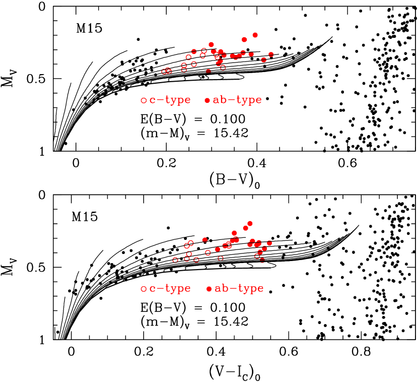
Figure 18.— Overlay of evolutionary tracks for core He-burning stars and the corresponding ZAHB onto the CMD for the HB and RGB populations of M 15 that have $0.0\leq M_{V}\leq 1.0$. The same RR Lyrae stars appear in both panels. The ZAHB (for [Fe/H] $=-2.3$ and [O/Fe] $=0.6$) is identical to the one that is compared with HST photometry of M 15 in the right-hand panel of Fig. 15, and with $VI_{C}$ observations of M 92 in Fig. 11.

Figure 19.— Plot of the measured periods of the $ab$- and $c$-type variables (filled and open circles, respectively) in M 3 as a function of $(B-V)_{m}$ (left-hand panel) and in M 15 as a function of both $(B-V)_{m}$ (middle panel) and $(V-I_{C})_{m}$ (left-hand panel).

This inconsistency is especially apparent if the ZAHB loci and associated evolutionary tracks are compared with the locations of the M 15 RR Lyrae, assuming intensity-weighted $\langle V\rangle_{i}$ magnitudes and magnitude-weighted $(B-V)_{m}$ or $(V-I_{C})_{m}$ colors for the variables. The upper panel of Figure 18 shows that many of the RR Lyrae have redder $(B-V)_{0}$ colors than the reddest ZAHB model, whereas all of the variables have bluer $(V-I_{C})_{0}$ colors than the reddest ZAHB model (see the lower panel). (Note that the same $ab$- and $c$-type variables are considered on both color planes.) Part of the explanation of this discrepancy could be that $(B-V)_{m}$ needs a larger blueward correction than $(V-I_{C})_{m}$ to represent the corresponding color of a static star, though this should not amount to more than $\sim 0.02$ mag, judging from the results for M 3 by Cacciari et al. (2005). Errors in the adopted $(B-V)$–${T_{\rm eff}}$ transformations (from CV14) could also be a contributing factor. Alternatively, errors in the derived values of the mean magnitudes and/or colors may be primarily responsible for this conundrum.

In fact, the star-to-star scatter in the M 15 data is much larger than in the case of M 3. As illustrated in Figure 19, the periods of the variables in M 3 show a much tighter correlation with $(B-V)_{m}$ than those in M 15. Particularly disconcerting is the fact that many of the $c$-type variables in M 15 span a very wide range in color despite having nearly the same pulsation periods; these are the stars with $P\sim 0.38$ d. Interestingly, the variables in M 68, which appears to have the same [Fe/H] as M 15 to within 0.1 dex (Carretta et al. 2009a), also has a remarkable concentration of variables at a fixed period (see Catelan 2004, who provides some discusson of this anomaly in both clusters). Although helium abundance variations may provide a partial explanation, this is unlikely to be the primary explanation because the properties of the hotter first-overtone pulsators are considerably less dependent on $Y$ than the cooler fundamental-mode pulsators. This will become clear in the following discussion.

Because $B-V$ colors will generally be more problematic than $V-I_{C}$, and because we had satisfactory success explaining the properties of the RR Lyrae in M 92 when their effective temperatures were derived from $V-I_{C}$ colors, we decided to present just our analysis of $VI_{C}$ photometry of M 15. Our main goal, anyway, is to try to understand why the observed values of $\langle P_{ab}\rangle$ are so similar for M 92 and M 15, and this can be accomplished in a more robust way if the same color is used to derive the temperatures of their respective variable stars. (The brief examination that we did carry out of the $B-V$ data for M 15 suggests that the measured $(B-V)_{m}$ values must be reduced by $\mathrel{\hbox{\raise 2.58334pt\hbox{$>$}\kern-7.3194pt\lower 2.15277pt\hbox{$\sim$}}}0.03$ mag to obtain good consistency with the results presented below. Such offsets could be due, in part, to errors in the adopted color–${T_{\rm eff}}$ relations.)

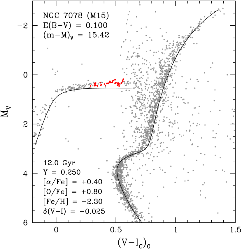
Figure 20.— As in the right-hand panel of Fig. 15, except that models for [O/Fe] $=0.8$ (instead of 0.6) have been fitted to the observed CMD of M 15. RR Lyrae stars have been plotted as small red dots.

It turns out that a ZAHB for [Fe/H] $=-2.3$ and [O/Fe] $=0.6$ (i.e., for an extra 0.2 dex above the amount implied by [$\alpha$/Fe] $=0.4$) does not extend far enough to the red in order for HB evolutionary tracks to explain the RR Lyrae if some/most of them have $Y>0.25$, so we opted to use models for [O/Fe] $=0.8$ in our analysis. This does not affect the ZAHB-based distance modulus, but it does imply a reduced turnoff age by $\approx 0.5$ Gyr. As shown in Figure 20, the best-fit isochrone for the higher oxygen abundance predicts an age of $\approx 12.0$ Gyr for M 15 if it has $(m-M)_{V}=15.42$ and $E(B-V)=0.10$. Under these assumptions, a ZAHB for $Y=0.25$, [Fe/H] $=-2.3$, and [O/Fe] $=0.8$ (with [m/Fe] $=0.4$ for the other $\alpha$-elements) provides quite a good fit to the faintest cluster HB stars. (Recall from § 3.2.1 that a 0.2 dex increase in [O/Fe] has only minor consequences for the predicted periods of RR Lyrae variables.)

Possible fits of ZAHB loci and the associated evolutionary tracks for the core He-burning phase are illustrated in Figure 21. The bottom panel shows that a ZAHB for $Y=0.25$ provides a good fit to the non-variable stars just to the blue of the instability strip and that all of the RR Lyrae are located well above this ZAHB. Indeed, many of the $ab$-type variables are located near, or past, the ends of tracks, where relatively few stars are expected because of the increasingly rapid rate of evolution as the central helium content is depleted (e.g., Pritzl et al. 2002). (Recall that the tracks end when $Y_{C}\approx 0.01$.) As discussed in § 1, the large number of variables has always been a strong argument that most of them cannot be highly evolved stars, but rather that the majority must be relatively close to their respective ZAHB locations. (Note that the selected stars represent only $\sim 25$–30% of the total number of RR Lyrae in M 15, which is especially rich in these variables; see Corwin et al. 2008.)

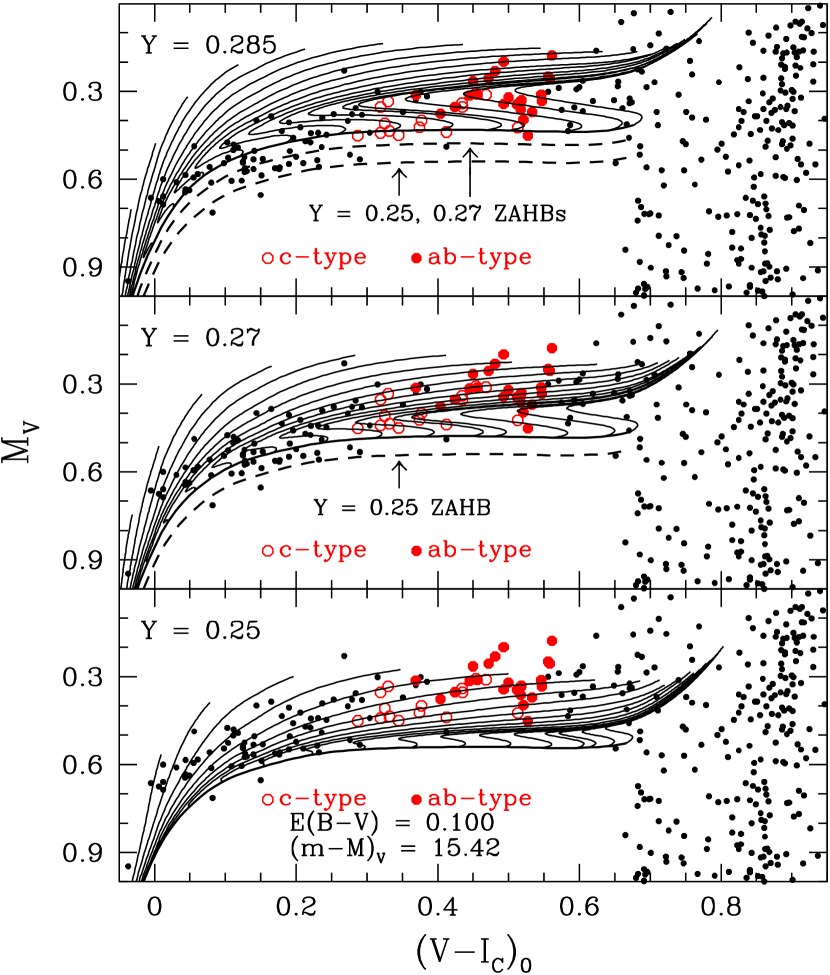
Figure 21.— Overlays of ZAHBs and evolutionary tracks for different helium abundances onto the HB population of M 15. Filled and open circles (in red) identify the $ab$- and $c$-type RR Lyrae, respectively. The dashed loci in the middle and upper panels reproduce the ZAHBs that appear in lower panels (for lower $Y$, as indicated). The reddening and distance modulus that are specified in the lower panel apply to all three panels.

Higher $Y$ is one way of achieving this since, as shown in the middle and upper panels of Fig. 21, many (or most) of the variables would be located along, or just above, ZAHBs for $Y\mathrel{\hbox{\raise 2.58334pt\hbox{$>$}\kern-7.3194pt\lower 2.15277pt\hbox{$\sim$}}}0.27$. This, together with the increased prominence of blue loops in tracks for a given mass and higher helium abundance, means that the masses of the RR Lyrae stars that are derived by interpolating within the evolutionary tracks will increase with increasing $Y$. (That the effect on the mass can be quite large for some of the stars is obvious from an inspection of Fig. 21.) Indeed, it is mainly through the mass terms in equations (1) and (2) that the predicted periods will be affected by the variable’s helium abundance. If all of the stars are at the same distance, subject to the same reddening, and have the essentially same metal abundances, the contributions to $\log\,P$ arising from the $\log(L/L_{\odot})$, $\log\,{T_{\rm eff}}$, and $\log Z$ terms will be nearly, or entirely, independent of $Y$.

The fact that the coefficients of the mass terms are relatively small in equations (1) and (2) makes it difficult to use the observed periods to obtain a clear separation of the M 15 variables into groups of normal (i.e., close to primordial), intermediate, and high helium abundances. At best, predicted periods will be uncertain by $\delta P\approx\pm 0.03$ d, which corresponds (for instance) to an error bar of $\sim 0.01$ dex in the $\log{T_{\rm eff}}$ value of an individual RR Lyrae. Consequently, the models for $Y=0.25$, 0.27, and 0.285 are likely to fare equally well, or equally poorly, in explaining the observed periods — though one can anticipate that, due to vagaries in the data, one helium abundance might be favored over the others depending on whether the predicted period for that $Y$ is just inside or just outside its assumed $1\,\sigma$ uncertainty.

Figure 22.— Similar to Fig. 6 (for M 3) and Fig. 10 (for M 92), except that the M 15 variables are considered. Symbols identify RR Lyrae with periods that are reproduced to within $\pm 0.03$ d by models for $Y=0.25$ (open circles), 0.27 (crosses), or 0.285 (open squares). Filled circles are used if the models for all three values of $Y$ satisfy this criterion, while filled triangles represent stars for which the discrepancies between the predicted and observed periods are $>0.03$ d. The $\delta\log{T_{\rm eff}}$ offsets that were applied to the models for $Y=0.25$, 0.27, and 0.285 so that the predicted values of $\langle P_{ab}\rangle$ and $\langle P_{c}\rangle$ agree with the observed values are given in the lower right-hand corner. The differences between the predicted and observed periods have $\sigma(\Delta P_{ab})=0.050$ d and $\sigma(\Delta P_{c})=0.030$ d. Averages of the predicted periods and the stellar properties have been adopted for those variables that are plotted as filled circles, the superposition of two different symbols, or filled triangles.

These remarks anticipate the results of our interpolations, which are presented in Figure 22. This shows that our models for any of the three values of $Y$ that we have considered are able to reproduce the observed pulsation periods of 6 RR Lyrae (the ones represented by filled circles) to within $\pm 0.03$ d (our adopted consistency criterion). Not surprisingly, most of them are $c$-type variables, for which the range in the interpolated masses from the grids of HB tracks for $Y=0.25$, 0.27, and 0.285 is typically $\mathrel{\hbox{\raise 2.58334pt\hbox{$<$}\kern-7.74998pt\lower 2.15277pt\hbox{$\sim$}}}0.05{\cal M_{\odot}}$, as compared with a range that can be as large as $\sim 0.1{\cal M_{\odot}}$ for many of the cooler $ab$-type variables. The periods of a few other variables can be explained quite well by models for $Y=0.25$ and 0.27, which are identified by the superposition of open circles and crosses, while a preference for just one of the three values of $Y$ is obtained for several other stars (those plotted as open circles, open squares, or crosses). Satisfactory explanations of the measured periods could not be obtained for those stars that are represented by filled triangles.

There were a few variables in the initial sample for which the discrepancies between the predicted and observed periods were even larger than those obtained for any of the stars plotted in Fig. 22. They were dropped from consideration prior to performing the analysis that produced the results shown in this figure, because their removal made it much easier to achieve consistency between the predicted and observed values of $\langle P_{ab}\rangle$ and $\langle P_{c}\rangle$. As indicated in Fig. 22, the $\delta\log{T_{\rm eff}}$ adjustments that were applied to the RR Lyrae temperatures to attain this consistency are all quite small. There is no reason to retain the extreme outliers in the sample anyway, as it is not possible to explain, in the context of the adopted stellar models, why the periods implied by their CMD locations would be so much larger or smaller than the observed periods (by $\sim 0.10$–0.22 d) when reasonably good agreement is found for the majority of the variables. (The particularly problematic RR Lyrae stars are the fundamental pulsators V21, V47, and V60, and the first-overtone pulsators V70 and V120. Further study of these variables is clearly needed to to understand their apparently anomalous properties.)

In order to make our analysis of the M 15 variables as close to a purely differential study with respect to M 92 as possible, we fitted the same $Y=0.25$, [Fe/H] $=-2.3$, [O/Fe] $=0.8$ models that we have employed for M 15 to observations of M 92. By interpolating within the corresponding grids of HB tracks, we found that the observed values of $\langle P_{ab}\rangle$ and $\langle P_{c}\rangle$ for M 92 could be reproduced if the temperatures of the $ab$- and $c$-type pulsators were adjusted by $\delta\log{T_{\rm eff}}=0.0$ and $+0.0069$, respectively. These determinations differ by $\sim 0.004$ from the adjustments adopted in the construction of Fig. 10, which is essentially identical with the plot that is obtained on the assumption of models that assume [O/Fe] $=0.8$. Small shifts in the RR Lyrae ${T_{\rm eff}}$ scale that are needed to reconcile the predicted and observed values of $\langle P_{ab}\rangle$ and $\langle P_{c}\rangle$ in M 15, on the one hand, and in M 92, on the other, are plausibly due to differences in the photometric zero-points and/or in the respective magnitude-weighted colors.

Although our analysis suggests that many of the RR Lyrae in M 15 have a higher helium abundance than those in M 92, the large number of variables in M 15 provides more compelling support for the same conclusion. It is widely accepted that, as in the case of M 3, “the bulk of the RR Lyrae in M 15 are in an early stage of evolution from the ZAHB” (Bingham et al. 1984). However, the ZAHB that fits the nonvariable blue HB stars in M 15, which provides an equally good fit to their counterparts in M 92, is considerably fainter than the lowest-luminosity RR Lyrae (in both clusters). Whereas the small number of variables in M 92 is consistent with them being evolved stars from ZAHB structures well to the blue of the instability strip, the large number of variables in M 15, which have similar or greater luminosities than those residing in M 92, argues that there must be at least two distinct ZAHB populations in M 15. The most likely explanation for the offset in luminosity between them is a difference in the abundance of helium — a conclusion that is supported by our detailed examination of the cluster RR Lyrae stars. [The extended blue tail of M 15’s HB, which contains a non-uniform distribution of stars with gaps at some magnitudes, has long been thought to indicate the presence of multiple stellar populations (see, e.g., Buonanno et al. 1985, Crocker et al. 1988). These observations may be indicative of even larger helium abundance variations than the $\delta Y\sim 0.03$–04 that is probably sufficient to account for the stars along the flat part of its HB.]

4. Summary and Discussion

Table 1Mean Properties of the M 3, M 15, and M 92 RR Lyrae Stars

Name		$\langle P\rangle$	$\sigma$	$\langle P\rangle$	$\sigma$	$\langle\log\,T_{\rm eff}\rangle$	$\sigma$	$\langle{\cal M}/{{\cal M}_{\odot}}\rangle$	$\sigma$	$\langle M_{\rm bol}\rangle$	$\sigma$	$\langle M_{V}\rangle$	$\sigma$	$Z$
$ab$-type
M 3		0.568	0.067	0.568	0.075	3.812	0.012	0.656	0.016	0.534	0.058	0.583	0.056	$7.623\times 10^{-4}$
M 15		0.654	0.060	0.654	0.068	3.813	0.013	0.706	0.051	0.257	0.055	0.326	0.058	$2.466\times 10^{-4}$
M 92		0.645	0.033	0.645	0.042	3.815	0.005	0.673	0.011	0.283	0.042	0.347	0.041	$1.786\times 10^{-4}$
$c$-type
M 3		0.336	0.050	0.336	0.058	3.855	0.013	0.630	0.016	0.514	0.104	0.520	0.102	$7.623\times 10^{-4}$
M 15		0.365	0.038	0.365	0.046	3.848	0.014	0.712	0.038	0.363	0.060	0.395	0.052	$2.466\times 10^{-4}$
M 92		0.352	0.050	0.352	0.053	3.860	0.016	0.662	0.005	0.340	0.040	0.360	0.029	$1.786\times 10^{-4}$
aObserved mean period (in d) of the samples of RR Lyrae considered in this study.
bPredicted mean period (in d) of the samples of RR Lyrae considered in this study.

Mainly during the last 3 decades of the 20^th century, but continuing to the present day, many investigators in the GC, stellar evolution, and variable star communities have tried to understand the Oosterhoff (1939, 1944) dichotomy, particularly as regards M 3 (Oo type I) and M 15 (Oo II) because they are so rich in RR Lyrae. No one worked harder to explain the difference in the mean periods of their RR Lyrae populations than Allan Sandage and, in the end, it seems that his solution to this problem, that M 15 RR Lyrae stars have higher helium abundances than those in M 3 (see Sandage et al. 1981), stands a good chance of being the right answer. [Prior to $\sim 2005$, GCs were considered to be simple stellar populations in which all stars within each cluster were thought to be coeval and essentially chemically homogeneous, aside from the ubiquitous star-to-star variations in CN. It was generally assumed that helium did not vary, given that the application of the R-method (Iben 1968) yielded very similar helium abundances, $Y\approx 0.25$, for most clusters, especially those with red HBs (e.g., see Salaris et al. 2004, and references therein). Consequently, everyone viewed the possibility that $Y$ varies inversely with [Fe/H], which also seems counter-intuitive from a chemical evolution perspective, with considerable skepticism. Only recently has it been established that GCs contain multiple, chemically distinct stellar populations that have, or probably have, different helium abundances. As mentioned in § 1, the most massive clusters have provided the most compelling evidence for such variations.]

To be sure, our apparent success in modeling the HBs of M 3, M 15, and M 92 is due in part to the improvements made to both the stellar models over the years and the theoretical relations that describe the dependence of the period on luminosity, mass, ${T_{\rm eff}}$, and metallicity for the fundamental and the first-overtone pulsators (Marconi et al. 2015). With just minor adjustments (well within the associated uncertainties) to the RR Lyrae ${T_{\rm eff}}$ scale (or, equivalently, to the coefficients of $\log{T_{\rm eff}}$ in these equations), it is possible to reproduce the observed values of $\langle P_{ab}\rangle$ and $\langle P_{c}\rangle$ quite well. The advances that have been made likely explain why we find $\delta Y$(M 15 minus M 3) $\sim 0.03$, as compared with a difference closer to 0.05, in the same sense, that was derived by Sandage et al. (1981, also see ).

Table 1 lists the observed and predicted values of $\langle P_{ab}\rangle$ and $\langle P_{c}\rangle$ and their standard deviations ($\sigma$), as derived from the individual RR Lyrae stars in each cluster, along with the mean values and standard deviations of the temperatures, masses, absolute bolometric magnitudes, and absolute $V$-band magnitudes of the variables. (Note that the mean periods which are calculated from equations (1) and (2) on the assumption of the quantities given in the sixth, eighth, tenth, and last columns agree very well with the values listed in the fourth column.) Nearly the same value of $\langle\log\,T_{\rm eff}\rangle$ is obtained for the $ab$-type RR Lyrae ($\approx 3.815$) and $c$-type variables ($\approx 3.855$) in all three clusters.

In addition, the variables in M 15 are predicted to have higher mean masses (and significantly larger mass dispersions) than those in M 92 and M 3. Consistent with the plots of the RR Lyrae on various CMDs (see, e.g., Figs. 5, 12, and 18), the magnitudes of the first-overtone pulsators in M 3 have the largest standard deviations, while the luminosity dispersions of both the $ab$- and $c$-type RR Lyrae are the smallest in M 92. Not surprisingly, the variables in M 15 and M 92 have brighter absolute magnitudes by $\mathrel{\hbox{\raise 2.58334pt\hbox{$>$}\kern-7.3194pt\lower 2.15277pt\hbox{$\sim$}}}0.2$ mag than those in M 3. (As one would expect, the tabulated properties have some dependence on the samples of RR Lyrae that are considered. For instance, had we retained the most problematic M 15 variables in our analysis, we would have obtained $\langle M_{\rm bol}\rangle$ $=0.241\pm 0.068$ and $\langle M_{V}\rangle$ $=0.313\pm 0.065$ for the $ab$-type variables in this cluster, as well as $\langle M_{\rm bol}\rangle$ $=0.354\pm 0.062$ and $\langle M_{V}\rangle$ $=0.392\pm 0.053$ for its first-overtone pulsators.)

The importance of taking diffusive processes into account should be appreciated. One of the consequences of diffusion is that, due to the settling of helium in the interiors of stars during their main sequence and subgiant evolution, the envelope helium abundance after the first dredge-up (i.e., after the convective envelope has reached its maximum depth on the lower RGB) is predicted to be less than the initial helium content by $\delta Y\sim 0.003$ (assuming a $0.8{\cal M_{\odot}}$ model for [Fe/H] $=1.55$). If diffusion is ignored, the envelope helium abundance is predicted to be higher than the initial abundance by $\delta Y\sim 0.01$. Since the luminosity of the HB is a sensitive function of $Y$ (see Figs. 8, 21), ZAHBs will be significantly fainter, implying reduced ZAHB-based distance moduli, if diffusion is treated. (As discussed in § 3.1, the value of $(m-M)_{V}=15.04$ that we have derived for M 3 using ZAHB models satisfies the constraint provided by current calibrations of the RR Lyrae standard candle quite well.)

Furthermore, the prominence of blue loops in post-ZAHB evolutionary tracks depends quite strongly on the helium abundance (see, e.g., Fig. 21). This has important ramifications for the intermingling of $ab$-type and $c$-type RR Lyrae. For instance, as discussed in § 3.1, there appears to be very little overlap of the colors of these variables in M 3 (see Fig. 5), which suggests that blue loops must be small or non-existent if the transition between fundamental and first-overtone pulsation, or vice versa, depends on the direction in which the core He-burning stars are evolving through the instability strip (the so-called “hysteresis effect”; see van Albada & Baker 1973, and especially the very instructive plots provided by and ). Our diffusive models for an initial helium abundance of $Y=0.250$ predict small blue loops (see Fig. 5), though better consistency with the observations would be obtained if they were even smaller, which suggests that a slightly lower value of $Y$ should be adopted (but within the uncertainties of the primordial helium abundance) or that our models underestimate the rate at which settling occurs in stars.

Higher $Y$ by $\sim 0.013$, as predicted by non-diffusive stellar models, would result in extended blue loops, which seems incompatible with the fairly sharp boundary between the $ab$- and $c$-type variables in M 3. (The age of HD 140283 provides another argument that diffusion physics should not be neglected in stellar models; see § 3.2.2 and VandenBerg et al. 2014b.) There is no overlap of the colors of these RR Lyrae in M 92, nor is any expected because the evolution through the instability strip is clearly in the direction from blue to red from ZAHB locations on the blue side of the instability strip (see Figs. 9, 11, 12). It is not clear what to make of the M 15 variables in this regard (see Fig. 21), partly because the magnitude-weighted colors derived by Corwin et al. (2008) seem particularly uncertain, and because it is not possible to unambiguously determine the helium abundances of the individual RR Lyrae stars. Further observational work to determine improved estimates of the colors of equivalent static stars of the M 15 variables would be very helpful, as would an extension, towards lower metallicities and additional bandpasses, of the theoretical studies of Bono et al. (1995) on the differences between different types of averages and the static magnitudes and colors.

As discussed by Arellano Ferro et al. (2015), a separation of the $ab$- and $c$-type RR Lyrae in terms of their colors is found in most GCs, irrespective of whether they are OoI or OoII systems. Notable exceptions are the OoI cluster NGC 3201 (Arellano Ferro et al. 2014) and the OoII clusters M 15 and $\omega$ Cen (see Sandage 1981). When there is a mixture of fundamental and first-overtone pulsators in a restricted color range within the instability strip, some of the variables are expected to be evolving from red to blue, and their periods should be decreasing with time, while others will be evolving in the opposite direction with positive period-change rates, $\Delta P/\Delta t$ (see Fig. 3 by Caputo et al. 1978).

In principle, it should be possible to use measurements of $\Delta P/\Delta t$ to determine the directions in which individual variables are evolving. In practice, however, this seems to be very difficult. As Corwin & Carney (2001) have concluded, period-change rates in M 3 appear to be due more to “noise” than to evolutionary effects. In their follow-up of the Corwin & Carney study, Jurcsik et al. (2012) noted that “positive and negative period-change rates with similar size are equally frequent at any period and brightness”. For instance, V1 and V10 have comparable mean magnitudes and colors, but the values of $\Delta P/\Delta t$ tabulated for them by Jurcsik et al. are $-0.417$ d/Myr and $+0.343$ d/Myr, respectively. These stars should both have increasing periods judging from their CMD locations, which are well above the ZAHB, relative to our evolutionary sequences. The same can be said of even brighter variables, and yet, as reported by Jurcsik et al., none of the four brightest RR Lyrae in M 3 have $\Delta P/\Delta t>0.0$. This includes the brightest $ab$-type variable in our sample, V42, which has a period-change rate of $-1.132$ d/Myr. In view of such results, and the possible concerns with the mean magnitudes and colors of M 15 variables mentioned above, we have not attempted to pursue this line of investigation — though it may be worthwhile to do so when improved data become available.

Being able to explain the RR Lyrae in M 3 and M 92 so well provides valuable support for our determinations of their distance moduli and ages. We find no compelling evidence for helium abundance variations in either cluster from our analysis of the variable stars, though star-to-star differences at the level of $\delta Y\mathrel{\hbox{\raise 2.58334pt\hbox{$<$}\kern-7.74998pt\lower 2.15277pt\hbox{$\sim$}}}0.02$ would be very difficult to detect. Our analysis suggests that the faintest HB stars on the blue side of the instability strip and some of the RR Lyrae in M 15 represent an M 92-like population. The fact that the difference in magnitude between these stars and the turnoff is identical to within measuring uncertainties in both clusters leads us to conclude that M 15 and M 92 are coeval (as most previous studies have found). However, M 15 appears to contain additional populations of stars with higher helium abundances, up to at least $Y\sim 0.29$ in the vicinity of the instability strip and possibly to higher values along the extended blue tail of the cluster HB. (Fits of isochrones to the turnoff photometry on the assumption of ZAHB-based distance moduli suggest that M 3, M 15, and M 92 all have ages of $\approx 12.5$ Gyr, depending on the assumed CNO abundances. It seems unlikely, in fact, that GCs are as old as the field halo subgiant HD 140283 — which is not implausible given the recent discovery of a galaxy at a redshift $z=11.1$ that seems to have built-up a stellar mass of $\sim 10^{9}{\cal M_{\odot}}$ within just $\sim 400$ Myr after the Big Bang; see Oesch et al. 2016.)

Our explanation of the M 15 RR Lyrae does raise an important question: why are the ZAHB stars with higher helium abundances distributed to redder colors than those for $Y\approx 0.25$? Possible answers to this question are (i) mass loss rates vary inversely with $Y$, though we are unaware of any empirical or theoretical support for this suggestion, (ii) the abundances of the CNO elements are higher in stars with increased helium abundances, (iii) the stars with higher $Y$ are somewhat younger than those with normal $Y$, or (iv) some combination of these possibilities. Jang et al. (2014) have suggested that second generation stars would have enhanced helium and CNO abundances though, in their proposed explanation of the Oosterhoff dichotomy, the different generations of stars would span different color ranges. We see no evidence that this is the case; indeed, a ZAHB for $Y=0.25$ appears to provide a good fit to the faintest HB stars at all $(V-I_{C})_{0}\mathrel{\hbox{\raise 2.58334pt\hbox{$<$}\kern-7.74998pt\lower 2.15277pt\hbox{$\sim$}}}0.3$, where stars with higher helium are presumably also found.

More importantly, there is very little spectroscopic evidence for variations in the total CNO abundance in M 15. Athough they studied only a few giants, Sneden et al. (1997) found that C$+$N$+$O is constant to within the measurement uncertainties in 5 of the 6 stars in their sample. One giant apparently has much higher CNO, given that the derived nitrogen abundance corresponds to [N/Fe] $\sim+1.6$. However, previous studies of much larger samples of upper RGB stars concluded that there are no real differences in the C and N abundances of M 15 and M 92 (Carbon et al. 1982, Trefzger et al. 1983). Both clusters do show a steep decline of [C/Fe] with [Fe/H] (also see Bellman et al. 2001), but C–N and O–N cycling together with deep mixing (Denissenkov & Denissenkova 1990, Langer et al. 1993, Denissenkov & VandenBerg 2003) can explain those observations without requiring star-to-star variations in CNO (Pilachowski 1988, Sneden et al. 1991, Cohen et al. 2005).

Although C$+$N$+$O seems to be approximately constant, the observed variations of CN in present-day main sequence and subgiant stars, as well as star-to-star differences in Mg and Al at any luminosity (e.g., see the relevant studies of M 92 and M 15 by King et al. 1998, Grundahl et al. 2000, Cohen et al. 2005, Carretta et al. 2009b), is an entirely different issue because they cannot be produced by evolutionary processes within lower mass stars. Such variations must have arisen during an extended period (or possibly successive epochs) of star formation at early times or, if the stars currently observed within a given GC are coeval, they must have been present in the gas out of which the cluster stars formed. That the helium-enhanced stars in M 15 appear to populate ZAHBs that extend to much redder colors than the ZAHB which fits the faintest stars to the blue of the instability strip suggests that the spread in stellar ages may be larger in M 15 than in M 92 or M 3. [Regardless of which scenario provides the most correct explanation, there is little doubt that H-burning nucleosynthesis at very high temperatures ($\sim 75\times 10^{6}$ K, as predicted for supermassive stars; see Denissenkov & Hartwick 2014) is responsible for the observed abundance correlations and anti-correlations, including ratios of the abundances of magnesium isotopes (Denissenkov et al. 2015).]

The potential importance of rotation for our understanding of the HBs in GCs should be kept in mind as well. In the few studies that have been undertaken during the past few decades to measure the rotation of member stars, unexpectedly high rotational velocities have been determined for blue HB stars in the most metal-poor systems (specifically, M 92; see Cohen & McCarthy 1997) and in higher metallicity GCs with extremely blue HBs, including M 13 (Peterson 1983) and NGC 288 (Peterson 1985). A spread of rotational velocities in the precursor red giants would seem to be the most probable cause of the variations in total mass along GC horizontal branches, and the average mass loss could therefore be related to the average rotational velocity in upper RGB stars. The fact that the decline of the surface carbon abundance with increasing luminosity along the giant branch is much more pronounced in M 13 (Smith & Martell 2003) and most, if not all, of the extremely metal-deficient GCs (Martell et al. 2008) than in metal-rich clusters can hardly be a coincidence. Sweigart & Mengel (1979) have shown that such observations can be explained by rotationally driven deep-mixing, which is expected to become less important as the metallicity increases due to the concomitant increase in the mean molecular weight gradient near the H-burning shell. (Red giants in NGC 288, which has a higher [Fe/H] than M 13 by $\sim 0.5$ dex, mainly show a bimodality of CN strengths with only a hint of a decline of C and O with increasing luminosity; see Smith & Langland-Shula 2009.)

The next paper in the series will carefully examine the differences in the CMDs of M 3 and M 13 to try to explain why these two clusters have such different HB morphologies, despite having nearly identical [Fe/H] values. Synthetic HB populations will be presented in this investigation, which will include an analysis of, among other things, the detailed distribution of mass along the observed HBs of these two systems, which is an important and controversial issue; see, e.g., Caloi & D’Antona (2008) and Valcarce & Catelan (2008).

References

- Afşar et al. (2016) Afşar, M., Sneden, C., Frebel, A., et al. 2016, astro-ph, arXiv:1601.02450
- Anderson et al. (2009) Anderson, J., Piotto, G., King, I. R., Bedin, L. R., & Guhathakurta, P. 2009, ApJL, 697, L58
- Amarsi et al. (2015) Amarsi, A. M., Asplund, M., Collet, R., & Leenaarts, J. 2015, MNRASL, 454, L11
- Arellano Ferro et al. (2014) Arellano Ferro, A., Ahumada, J. A., Calderón, J. H., & Kains, N. 2014, Rev. Mex. Astron. Astrophys., 50, 307
- Arellano Ferro et al. (2015) Arellano Ferro, A., Mancera Piña, Bramich, D. M., Giridhar, S., Ahumada, J. A., Kains, N., & Kuppuswamy, K. 2015, MNRAS, 727, 727
- Asplund et al. (2009) Asplund, M., Grevesse, N., Sauval, A. J., & Scott, P. 2009, ARAA, 47, 481
- Behr (2003) Behr, B. B. 2003, ApJS, 149, 67
- Bellini et al. (2013) Bellini, A., Piotto, G., Marino, A. P., et al. 2013, ApJ, 765, 3
- Bellman et al. (2001) Bellman, S., Briley, M. M., Smith, G. H., & Claver, C. F. 2001, PASP, 113, 326
- Bennett et al. (2013) Bennett, C. L., Larson, D., Weiland, J. L., et al. 2013, ApJS, 208, 20
- Bingham et al. (1984) Bingham, E. A., Cacciari, C., Dickens, R. J., & Fusi Pecci, F. 1984, MNRAS, 209, 765
- Bond et al. (2013) Bond, H. E., Nelan, E. P., VandenBerg, D. A., Schaefer, G. H., & Harmer, D. 2013, ApJL, 765, L12
- Bono et al. (1995) Bono, G., Caputo, F., & Stellingwerf, R. F. 1995, ApJS, 99, 263
- Brasseur et al. (2010) Brasseur, C. M., Stetson, P. B., VandenBerg, D. A., Casagrande, L., Bono, G., & Dall’Ora, M. 2010, AJ, 140, 1672
- Buchler & Kolláth (2011) Buchler, J. R., & Kolláth, Z. 2011, ApJ, 731, 24
- Buonanno et al. (1985) Buonanno, R., Corsi, C. E., & Fusi Pecci, F. 1985, A&A, 145, 97
- Buonanno et al. (1998) Buonanno, R., Corsi, C. E., Pulone, L., Fusi Pecci, F., & Bellazzini, M. 1998, A&A, 333, 505
- Cacciari et al. (2005) Cacciari, C., Corwin, T. M., & Carney, B. W. 2005, AJ, 129, 267
- Caloi & D’Antona (2008) Caloi, V., & D’Antona, F. 2008, ApJ, 673, 847
- Caputo et al. (1978) Caputo, F., Castellani, V., & Tornambè, A. 1978, A&A, 67, 107
- Carbon et al. (1982) Carbon, D. F., Romanishin, W., Langer, et al. 1982, ApJS, 49, 207
- Carney (1996) Carney, B. W. 1996, PASP, 108, 900
- Carretta (2015) Carretta, E. 2015, ApJ, 810, 148
- Carretta et al. (2009a) Carretta, E., Bragaglia, A., Gratton, R. G., D’Orazi, V., & Lucatello, S. 2009a, A&A, 508, 695
- Carretta et al. (2009b) Carretta, E., Bragaglia, A., Gratton, R. G., & Lucatello, S. 2009b, A&A, 505, 139
- Carretta et al. (2005) Carretta, E., Gratton, R. G., Lucatello, S., Bragaglia, A., & Bonifacio, P. 2005, A&A, 433, 597
- Casagrande et al. (2010) Casagrande, L., Ramírez, I., Meléndez, J., Bessell, M., & Asplund, M. 2010, A&A, 512, 54
- Casagrande & VandenBerg (2014) Casagrande, L., & VandenBerg, D. A. 2014, MNRAS, 444, 392 (CV14)
- Cassisi et al. (2008) Cassisi, S., Salaris, M., Pietrinferni, A., Piotto, G., Milone, A. P., Bedin, L. R., & Anderson, J. 2008, ApJ, 672, 115
- Catelan (1992) Catelan, M. 1992, A&A, 261, 457
- Catelan (1993) Catelan, M. 1993, A&AS, 98, 547
- Catelan (2004) Catelan, M. 2004, ApJ, 600, 409
- Catelan (2009) Catelan, M. 2009, Ap&SS, 320, 261
- Catelan et al. (2009) Catelan, M., Grundahl, F., Sweigart, A. V., Valcarce, A. A. R., & Cortés, C. 2009, ApJL, 695, L97
- Cayrel et al. (2004) Cayrel, R., Depagne, E., Spite, M., et al. 2004, A&A, 416, 1117
- Chaboyer et al. (1996) Chaboyer, B., Demarque, P., Kernan, P. J., Krauss, L. M., & Sarajedini, A. 1996, MNRAS, 283, 683
- Chaboyer et al. (2013) Chaboyer, B., Feiden, G., Benedict, G. F., et al. 2013, in Advancing the Physics of Cosmic Distances, IAU Symp. 289, ed. R. de Grijs (Cambridge Univ. Press; Cambridge, U.K.), p. 87
- Clement et al. (2001) Clement, C., Muzzin, A., Dufton, Q., et al. 2001, AJ 122, 2587
- Clementini et al. (2003) Clementini, G., Gratton, R. G., Bragaglia, A., et al. 2003, AJ, 125, 1309
- Cohen (2011) Cohen, J. G. 2011, ApJL, 740, L38
- Cohen et al. (2005) Cohen, J. G., Briley, M. M., & Stetson, P. B. 2005, AJ, 130, 177
- Cohen & Kirby (2012) Cohen, J. G., & Kirby, E. N. 2012, ApJ, 760, 86
- Cohen & McCarthy (1997) Cohen, J. G., & McCarthy, J. K. 1997, AJ, 113, 1353
- Cohen & Meléndez (2005) Cohen, J. G., & Meléndez, J. 2005, AJ, 129, 303
- Constantino et al. (2015) Constantino, T., Campbell, S. W., Christensen-Dalsgaard, J., Lattanzio, J. C., & Stello, D. 2015, MNRAS, 452, 123
- Constantino et al. (2016) Constantino, T., Campbell, S. W., Lattanzio, J., & van Duijneveldt, A. 2016, MNRAS, 456, 3866
- Corwin et al. (2008) Corwin, T., Borissova, J., Stetson, P. B., Catelan, M., Smith, H. A., Kurtev, R., & Stephens, A. W. 2008, AJ, 135, 1459
- Corwin & Carney (2001) Corwin, T. M., & Carney, B. W. 2001, AJ, 122, 3183
- Creevey et al. (2015) Creevey, O. L., Thévenin, F., Berio, P., et al. 2015, A&A, 575, A26
- Crocker et al. (1988) Crocker, D. A., Rood, R. T., & O’Connell, R. W. 1988, ApJ, 332, 236
- Cyburt et al. (2010) Cyburt, R. H., Amthor, A. M., Ferguson, R., et al. ApJS, 189, 240
- Da Costa et al. (2013) Da Costa, G. S., Norris, J. E., & Yong, D. 2013, ApJ, 769, 8
- D’Alessandro et al. (2011) D’Alessandro, E., Salaris, M., Ferraro, F. R., et al. 2011, MNRAS, 410, 694
- Dell’Omodarme et al. (2012) Dell’Omodarme, M., Valle, g., Degl’Innocenti, S., & Prada Moroni, P. G. 2012, A&A, 540, A26
- Denissenkov & Denissenkova (1990) Denissenkov, P. A., & Denissenkova, S. N. 1990, Sov. Astron. Lett., 16, 275
- Denissenkov & Hartwick (2014) Denissenkov, P. A., & Hartwick, F. D. A. 2014, MNRASL, 437, L21
- Denissenkov & VandenBerg (2003) Denissenkov, P. A., & VandenBerg, D. A. 2003, ApJ, 593, 509
- Denissenkov et al. (2015) Denissenkov, P. A., VandenBerg, D. A., Hartwick, F. D. A., Herwig, F., Weiss, A., & Paxton, B. 2015, MNRAS, 448, 3314
- Di Criscienzo et al. (2010) Di Criscienzo, M., Ventura, P., D’Antona, F., Milone, A. P., & Piotto, G. 2010, MNRAS, 408, 999
- Dobrovolskas et al. (2015) Dobrovolskas, V., Kuc̆inskas, A., Bonifacio, P., Caffau, E., Ludwig, H.-G., Steffen, M., & Spite, M. 2015, A&A, 576, A128
- Dorman (1992) Dorman, B. 1992, ApJS, 81, 221
- Dotter et al. (2008) Dotter, A., Chaboyer, B., Jevremovíc, D., Kostov, V., Baron, E., & Ferguson, J. W. 2008, ApJS, 178, 89.
- Dotter et al. (2010) Dotter, A., Sarajedini, A., Anderson, J., et al. 2010, ApJ, 708, 698
- Durrell & Harris (1993) Durrell, P. R., & Harris, W. E. 1993, AJ, 105, 1420
- Eggleton (1971) Eggleton, P. P. 1971, MNRAS, 151, 351
- Ferguson et al. (2005) Ferguson, J. W., Alexander, D. R., Allard, F., et al. 2005, ApJ, 623, 585
- Ferraro et al. (2006) Ferraro, F. R., Valenti, E., Straniero, O., & Origlia, L. 2006, ApJ, 642, 225
- Formicola et al. (2004) Formicola, A., Imbriani, G., Costantini, H., et al. 2004, Phys. Let. B, 591, 61
- Gratton et al. (2012) Gratton, R. G., Carretta, E., & Bragaglia, A. A&ARv, 20, 50
- Gratton et al. (2013) Gratton, R. G., Lucatello, S., Sollima, A., et al. 2013, A&A, 549, A41
- Grundahl et al. (2000) Grundahl, F., VandenBerg, D. A., Bell, R. A., Andersen, M. I., & Stetson, P. B. 2000, AJ, 120, 1884
- Henyey et al. (1965) Henyey, L., Vardya, M. S., & Bodenheimer, P. 1965, ApJ, 142, 841
- Iben (1968) Iben, I., Jr. 1968, Nature, 220, 143
- King et al. (1998) King, J. R., Stephens, A., Boesgaard, A. M., & Deliyannis, C. 1998, AJ, 115, 666
- Komatsu et al. (2011) Komatsu, E., Smith, K. M., Dunkley, J., et al. 2011, ApJS, 192, 18
- Kopacki (2001) Kopacki, G. 2001, A&A, 369, 862
- Kraft & Ivans (2003) Kraft, R. P., & Ivans, I. I. 2003, PASP, 115, 143
- Harris (1996) Harris, W. E. 1996, AJ, 112, 1487
- Iben & Renzini (1984) Iben, I., Jr., & Renzini, A. 1984, Phys. Rep., 105, 329
- Iliadis et al. (2016) Iliadis, C., Karakas, A. I., Prantzos, N., Lattanzio, J. C., & Doherty, C. L. 2016, ApJ, 818, 98
- Jang & Lee (2015) Jang, S., & Lee, Y.-W. 2015, ApJS, 218, 31
- Jang et al. (2014) Jang, S., Lee, Y.-W., Joo, S.-J., & Na, C. 2014, MNRASL, 443, L15
- Johnson & Pilachowski (2012) Johnson, C. I., & Pilachowski, C. A. 2012, ApJL, 754, L38
- Jurcsik et al. (2012) Jurcsik, J., Hajdu, G., Szeidl, B., et al. 2012, MNRAS, 419, 2173
- Krishna Swamy (1966) Krishna Swamy, K. S. 1966, ApJ, 145, 174
- Langer et al. (1993) Langer, G. E., Hoffman, R., & Sneden, C. 1993, PASP, 105, 301
- Larsen et al. (2015) Larsen, S. S., Baumgardt, H., Bastian, N., Brodie, J. P., Grundahl, F., & Strader, J. 2015, ApJ, 804, 71
- Leaman et al. (2013) Leaman, R., VandenBerg, D. A., & Mendel, J. T. 2013, MNRAS, 436, 122
- Lee et al. (1990) Lee, Y.-W., Demarque, P., & Zinn, R. 1990, ApJ, 350, 155
- Magic et al. (2013) Magic, Z., Collet, R., Asplund, M., et al. 2013, A&A, 573, A89
- Magic et al. (2015) Magic, Z., Weiss, A., & Asplund, M. 2015, A&A, 573, A89
- Marconi et al. (2015) Marconi, M., Coppola, G., Bono, G., et al. 2015, ApJ, 808, 50
- Marino et al. (2014) Marino, A. F., Milone, A. P., Przybilla, N., et al. 2014, MNRAS, 437, 1609
- Marta et al. (2008) Marta, M., Formicola, A., Gyürky, Gy., et al. 2008, Phys. Rev. C, 78, 022802
- Martell et al. (2008) Martell, S. L., Smith, G. H., & Briley, M. M. 2008, AJ, 136, 2522
- Mashonkina et al. (2011) Mashonkina, L., Gehren, T., Shi, J.-R., Korn, A. J., & Grupp, F. 2011, A&A, 528, A87
- Milone et al. (2012) Milone, A. P., Piotto, G., Bedin, L. R., et al. 2012, ApJ, 744, 58
- Milone et al. (2015) Milone, A. P., Marino, A. F., Piotto, G.. et al. 2015, ApJ, 808, 51
- Mucciarelli et al. (2012) Mucciarelli, A., Bellazzini, M., Ibata, R., et al. 2012, MNRAS, 426, 2889
- Mucciarelli et al. (2014) Mucciarelli, A., Livosi, L., Lanzoni, B., & Ferraro, F. R. 2014, ApJ, 786, 14
- Oesch et al. (2016) Oesch, P. A., Brammer, G., van Dokkum, P. G., et al. 2016, ApJ, 819, 129
- Oosterhoff (1939) Oosterhoff, P. Th. 1939, Observatory, 62, 104
- (103) Oosterhoff, P. Th. 1944, Bull. Astron. Inst. Neth., 10, 55
- Paxton et al. (2011) Paxton, B., Bildsten, L., Dotter, A., et al. 2011, ApJS, 192, 3
- Peterson (1983) Peterson, R. C. 1983, ApJ, 275, 737
- Peterson (1985) Peterson, R. C. 1985, ApJL, 294, L35
- Peterson et al. (1990) Peterson, R. C., Kurucz, R. L., & Carney, B. W. 1990, ApJ, 350, 173
- Pietrzyński et al. (2013) Pietrzyński, G., Graczyk, D., Gieren, W., et al. 2013, Nature, 495, 76
- Pilachowski (1988) Pilachowski, C. A. 1988, ApJL, 326, L57
- Piotto et al. (2007) Piotto, G., Bedin, L. R., Anderson, J., et al. 2007, ApJL, 661, L53
- Pont et al. (1998) Pont, F., Mayor, M., Turon, C., & VandenBerg, D. A. 1998, A&A, 329, 87
- Preston et al. (2006) Preston, G. W., Sneden, C., Thompson, I. B., Schectman, S. A., & Burley, G. S. 2006, AJ, 132, 85
- Pritzl et al. (2002) Pritzl, B. J., Smith, H. A., Catelan, M., & Sweigart, A. V. 2002, AJ, 124, 949
- Ramírez et al. (2010) Ramírez, I., Collet, R., Lambert, D. L., Allende Prieto, C., & Asplund, M. 2010, ApJL, 724, L223
- Renzini (1983) Renzini, A. 1983, Mem. Soc. Astron. Ital., 54, 335
- Renzini et al. (2015) Renzini, A., D’Antona, F., Cassisi, S., et al. 2015, MNRAS, 454, 4197
- Renzini & Fusi Pecci (1988) Renzini, A., & Fusi Pecci, F. 1988, ARA&A, 26, 199
- Roederer & Sneden (2011) Roederer, I. U., & Sneden, C. 2011, AJ, 142, 22
- Roederer & Thompson (2015) Roederer, I. U., & Thompson, I. B. 2015, MNRAS, 449, 3889
- Rood (1973) Rood, R. T. 1973, ApJ, 184, 815
- Rood (1984) Rood, R. T. 1984, in Observational Tests of the Stellar Evolution Theory, eds. A. Maeder & A. Renzini (Dordrecht: Reidel), 167
- Salaris & Cassisi (2015) Salaris, M., & Cassisi, S. 2015, A&A, 577, A60
- Salaris et al. (2016) Salaris, M., Cassisi, S., & Pietrinferni, A. 2016, A&A, 590, A64
- Salaris et al. (2002) Salaris, M., Cassisi, S., & Weiss, A. 2002, PASP, 114, 375
- Salaris et al. (2004) Salaris, M., Riello, M., Cassisi, S., & Piotto, G. 2004, A&A, 420, 911
- Samus et al. (2009) Samus, N. N., Kazarovets, E. V., Pastukhova, E. N., Tsvetkova, T. M., & Durlevich, O. V. 2009, PASP, 121, 1378
- Sandage (1981) Sandage, A. 1981, ApJ, 248, 161
- Sandage (1982) Sandage, A. 1982, ApJ, 252, 553
- Sandage et al. (1981) Sandage, A., Katem, B., & Sandage, M. 1981, ApJS, 46, 41
- Sarajedini et al. (2007) Sarajedini, A., Bedin, L. R., Chaboyer, B., et al. 2007, AJ 133, 1658
- Schlafly & Finkbeiner (2011) Schlafly, E. F., & Finkbeiner, D. P. 2011, ApJ, 737, 103
- Schlegel et al. (1998) Schlegel, D. J., Finkbeiner, D. P., & Davis, M. 1998, ApJ, 500, 525
- Serenelli & Weiss (2005) Serenelli, A., & Weiss, A. 2005, A&A, 442, 1041
- Smith et al. (2005) Smith, V. V., Cunha, K., Ivans, I. I., Lattanzio, J. C., Campbell, S., & Hinkle, K. H. 2005, ApJ, 633, 392
- Smith & Langland-Shula (2009) Smith, G. H., & Langland-Shula, L. E. 2009, PASP, 121, 1054
- Smith & Martell (2003) Smith, G. H., & Martell, S. M. 2003, PASP, 115, 1211
- Smith et al. (1996) Smith, G. H., Shetrone, M. D., Bell, R. A., Churchill, C. W., & Briley, M. M. 1996, AJ, 112, 1511
- Sneden et al. (2000) Sneden, C., Johnson, J., Kraft, R. P., Smith, G. H., Cowan, J. J., & Bolte, M. 2000, ApJL, 536, L85
- Sneden et al. (1991) Sneden, C., Kraft, R. P., Prosser, C. F., & Langer, G. E. 1991, AJ, 102, 2001
- Sneden et al. (1997) Sneden, C., Kraft, R. P., Shetrone, M. D., Smith, G. H., Langer, G. E., & Prosser, C. F. 1997, AJ, 114, 1964
- Sneden et al. (2000) Sneden, C., Pilachowski, C. A., & Kraft, R. P. 2000, AJ, 120, 1351
- Sobeck et al. (2011) Sobeck, J. A., Kraft, R. P., Sneden C., et al. 2011, AJ, 141, 175
- Sollima et al. (2014) Sollima, A., Cassisi, S., Fiorentino, G., & Gratton, R. G. 2014, MNRAS, 444, 1862
- Stetson (2000) Stetson, P. B. 2000, PASP, 112, 925
- Straniero et al. (2003) Straniero, O., Domínguez, I., Imbriani, G., & Piersanti, L. 2003, ApJ, 583, 878
- Sweigart & Mengel (1979) Sweigart, A. V., & Mengel, J. G. 1979, ApJ, 229, 624
- Sweigart et al. (1987) Sweigart, A. V., Renzini, A., & Tornambe, A. 1987, ApJ, 312, 762
- Trampedach & Stein (2011) Trampedach, R., & Stein, R. F. 2011, ApJ, 731, 78
- Trefzger et al. (1983) Trefzger, D. V., Langer, G. E., Carbon, D. F., Suntzeff, N. B., & Kraft, R. P. 1983, ApJ, 266, 144
- Valcarce & Catelan (2008) Valcarce, A. A. R., & Catelan, M. 2008, A&A, 487, 185
- Valcarce et al. (2016) Valcarce, A. A. R., Catelan, M., Alonso-García, J., Contreras Ramos, R., & Alves, S. 2016, A&A, 589, A126
- van Albada & Baker (1973) van Albada, T. S., & Baker, N. 1973, ApJ, 185, 477
- VandenBerg (1983) VandenBerg, D. A. 1983, ApJS, 51,29
- VandenBerg (1992) VandenBerg, D. A. 1992, ApJ, 391, 685
- VandenBerg (2000) VandenBerg, D. A. 2000, ApJS, 129, 315
- VandenBerg et al. (2012) VandenBerg, D. A., Bergbusch, P. A., Dotter, A., Ferguson, J. W., Michaud, G., Richer, J., & Proffitt, C. R. 2012, ApJ, 755, 15
- VandenBerg et al. (2014a) VandenBerg, D. A., Bergbusch, P. A., Ferguson, J. W., & Edvardsson, B. 2014a, ApJ, 794, 72 (V14)
- VandenBerg et al. (2014b) VandenBerg, D. A., Bond, H. E., Nelan, E. P., Nissen, P. E., Schaefer, G. H., & Harmer, D. 2014b, ApJ, 792, 110
- VandenBerg et al. (2013) VandenBerg, D. A., Brogaard, K., Leaman, R., & Casagrande, L. 2013, ApJ, 775, 134 (V13)
- VandenBerg et al. (2010) VandenBerg, D. A., Casagrande, L., & Stetson, P. B. 2010, AJ, 140, 1020
- VandenBerg et al. (2015) VandenBerg, D. A., Stetson, P. B., & Brown, T. M. 2015, ApJ, 805, 103
- VandenBerg et al. (2000) VandenBerg, D. A., Swenson, F. J., Rogers, F. J., Iglesias, C. A., & Alexander, D. R. 2000, ApJ, 532, 430
- Worley et al. (2013) Worley, C. C., Hill, V., Sobeck, J., & Carretta, E. 2013, A&A, 553, A47
- Yong et al. (2009) Yong, D., Grundahl, F., D’Antona, F., Karakas, A. I., Lattanzio, J. C., & Norris, J. E. 2009, ApJL, 695, L62
- Yong et al. (2014) Yong, D., Roederer, I. U., Grundahl, F., et al. 2014, MNRAS, 441, 3396
- Zinn & West (1984) Zinn, R., & West, M. J. 1984, ApJS, 55, 45