Fast and robust mesh generation on the sphere
Application to coastal domains.

Abstract

This paper presents a fast an robust mesh generation procedure that is able to generate meshes of the earth system (ocean and continent) in matters of seconds. Our algorithm takes as input a standard shape-file i.e. geospatial vector data format for geographic information system (GIS) software. The input is initially coarsened in order to automatically remove unwanted channels that are under a desired resolution. A valid non-overlapping 1D mesh is then created on the sphere using the Euclidian coordinates system $x,y,z$. A modified Delaunay kernel is then proposed that enables to generate meshes on the sphere in a straightforward manner without parametrization. One of the main difficulty in dealing with geographical data is the over-sampled nature of coastline representations. We propose here an algorithm that automatically unrefines coastline data. Small features are automatically removed while always keeping a valid (non-overlapping) geometrical representation of the domain. A Delaunay refinement procedure is subsequently applied to the domain. The refinement scheme is also multi-threaded at a fine grain level, allowing to generate about a million points per second on 8 threads. Examples of meshes of the Baltic sea as well as of the global ocean are presented.

1 Introduction

Traditional ocean models are based on finite differences schemes on Cartesian grids [8]. It is only recently that unstructured meshes have been used in ocean modeling [17, 23, 3], essentially using finite elements. One of the advantages of unstructured grids is their ability to conform to coastlines.

As unstructured grid ocean models began to appear, mesh generation algorithms were either specifically developed or simply adapted from classical engineering tools. [13] use the mesh generation tools of [10] on several subdomains to obtain a mesh of the world ocean, aiming at global scale tidal modeling. Further, [16] use a higher resolution version of the same kind of meshes with the state of the art FES2004 tidal model. [9] give two algorithms to generate meshes of coastal domains, and use them to model tides in the Gulf of Mexico. [14] show high-resolution meshes of the Great Barrier Reef (Australia). At the global scale, [15] and [7] developed specific algorithms to obtain meshes of the world ocean. More recently, we have developed a proper CAD model of ocean geometries [11]. This model relies on the stereographic projection of the sphere which is conformal i.e. it conserves angles. This approach has been quite successful up to now: we and other teams have applied it to numerous coastal domains [21, 12].

Our CAD approach has two major drawbacks. First, at least two maps are required to cover the whole sphere, making it awkward for atmosphere simulations for example. Then, using splines is maybe not the most robust/natural manner for describing coastlines: geographical information systems provide description of coastlines as series of non-overlapping closed polygons and using splines may lead to intersections.

Here, a new approach that addresses both issues is proposed.

A modified Delaunay kernel is first presented that allows to generate meshes on the unit sphere. Based on our recent paper [19], a multithreaded version of this new kernel has been implemented that allows to triangulate over one million points per second on the sphere on a standard quad-core laptop. This new approach does not rely on any parametrization and has all the proof structure of the usual Delaunay kernel (proof of termination, angle-optimality, polynomial complexity).

In this new approach, the most refined representation of coastlines available in the geographical system is used as input . A constrained Delaunay mesh of the whole data set is created using the new Delaunay procedure. This first mesh allows to automatically and robustly remove from the domain any water channel that has a width that is smaller than a given threshold (this threshold being possibly variable in space). This first step leads to a coarsened version of the shapes where locally small features have been removed. We show that our procedure produces a valid (non-overlapping) boundary description of the domain. Then, a one-dimensional mesh is created using the coarse geometry. Finally, a multi-threaded version of the edge-based Delaunay refinement procedure of [5] has been used to saturate the domain with points and triangles.

The developments that are presented here have been released as a self consisten open source code that can be used as a stand alone program or that can be plugged in other softwares such as Gmsh [6] or QGIS [18].

2 Delaunay triangulation on the sphere

Here we consider the unit 3D sphere $S$ centered at the origin ${\bf o}(0,0,0)$: $S=\{\mathbf{x}(x,y,z)\in\mathds{R}^{3}~{}|~{}x^{2}+y^{2}+z^{2}=1\}$. Any section of a sphere by a plane is a circle. We distinguish great circles that are sections of a sphere that diameter is equal to the diameter of the sphere and small circles that are any other section.

Consider two points $\mathbf{p}_{1}$ and $\mathbf{p}_{2}$ on the sphere. The shortest path between $\mathbf{p}_{1}$ and $\mathbf{p}_{2}$ is called the geodesic path. It can be shown that geodesic paths on the sphere are segments of a great circle. The geodesic distance between $\mathbf{p}_{1}$ and $\mathbf{p}_{2}$ is the length of the great circular arc joining $\mathbf{p}_{1}$ and $\mathbf{p}_{2}$. We call it $\mbox{d}(\mathbf{p}_{1},\mathbf{p}_{2})$.

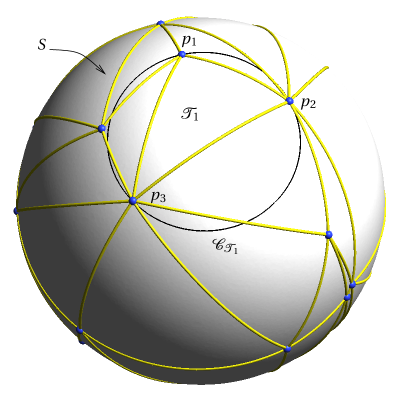
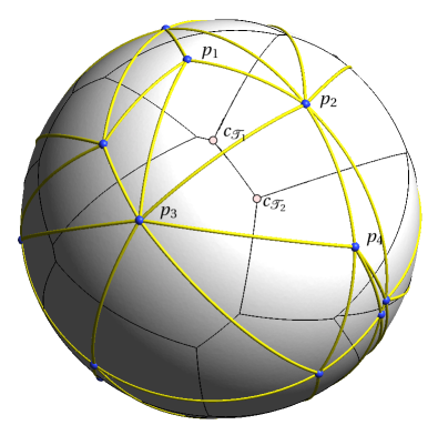
Fig. 1: Delaunay triangulation on a sphere. Spherical triangle $\mathcal{T}(\mathbf{p}_{1},\mathbf{p}_{2},\mathbf{p}_{3})$ is drawn with its spherical circumcircle $\mathcal{C}({\mathcal{T}})$ that is empty. Every triangle edge (in yellow, like $\mathbf{p}_{1}\mathbf{p}_{2}$) is a great circle.

A spherical triangle $\mathcal{T}_{1}(\mathbf{p}_{1},\mathbf{p}_{2},\mathbf{p}_{3})$ (see Figure 1) is a figure formed on the surface of a sphere by three great circular arcs intersecting pairwise in three vertices $\mathbf{p}_{1}$, $\mathbf{p}_{2}$ and $\mathbf{p}_{3}$. A spherical triangle is sometimes called an Euler triangle. Spherical triangles have an orientation that is computed as the sign of the volume $\|\mathbf{p}_{1},\mathbf{p}_{2},\mathbf{p}_{3},{\bf o}\|$ of tetrahedon $\mbox{t}(\mathbf{p}_{1},\mathbf{p}_{2},\mathbf{p}_{3},{\bf o})$ is positive, with ${\bf o}$ the center of $S$.

The circumcircle $\mathcal{C}_{\mathcal{T}_{1}}$ of the spherical triangle ${\mathcal{T}}_{1}$ is the small circle that is formed by the section of $S$ by the plane defined by points $\mathbf{p}_{1}$, $\mathbf{p}_{2}$ and $\mathbf{p}_{3}$ (see Figure 1). The circumcircle $\mathcal{C}_{\mathcal{T}_{1}}$ divides the sphere in two parts. Consider a point $\mathbf{p}$ of $S$:

• $p$ is inside $\mathcal{C}_{\mathcal{T}_{1}}$ if $\|\mathbf{p}_{1},\mathbf{p}_{2},\mathbf{p}_{3},\mathbf{p}\|<0$.

• $\mathbf{p}$ is outside $\mathcal{C}_{\mathcal{T}_{1}}$ if $\|\mathbf{p}_{1},\mathbf{p}_{2},\mathbf{p}_{3},\mathbf{p}\|>0$.

• $\mathbf{p}$ is on $\mathcal{C}_{\mathcal{T}_{1}}$ if $\|\mathbf{p}_{1},\mathbf{p}_{2},\mathbf{p}_{3},\mathbf{p}\|=0$.

There are exactly two antipodal points that are equidistant to $p_{1}$, $\mathbf{p}_{2}$ and $\mathbf{p}_{3}$. We define the spherical circumcenter of ${\mathcal{T}}_{1}$ as the point $\mathbf{c}_{\mathcal{T}_{1}}$ that is equidistant to $\mathbf{p}_{1}$, $\mathbf{p}_{2}$ and $\mathbf{p}_{3}$:

$$\mbox{d}(\mathbf{p}_{1},\mathbf{c}_{\mathcal{T}_{1}})=\mbox{d}(\mathbf{p}_{2},\mathbf{c}_{\mathcal{T}_{1}})=\mbox{d}(\mathbf{p}_{3},\mathbf{c}_{\mathcal{T}_{1}})$$

and that is inside $\mathcal{C}_{\mathcal{T}_{1}}$. This correspond to one of the two antipodal points that is the closets to $\mathbf{p}_{1}$, $\mathbf{p}_{2}$ and $\mathbf{p}_{3}$.

Consider a point set $P=\{\mathbf{p}_{1},\dots,\mathbf{p}_{n}\}$ of $n$ points of $S$. A triangulation $T(P)$ of $P$ is a set of $2n-4$ non overlapping spherical triangles

$$T(P)=\{{\mathcal{T}}_{1},{\mathcal{T}}_{2},\dots,{\mathcal{T}}_{2n-4}\}$$

that exactly covers $S$ with all points of $P$ being among the vertices of the triangulation.

A spherical triangle $\mathcal{T}_{j}$ is Delaunay if its circumcircle is empty i.e. if no point $\mathbf{p}_{i}$ of $P$ lies inside $\mathcal{T}_{j}$. The Delaunay triangulation $\mbox{DT}(P)$ is such that every triangle $\mathcal{T}_{j}$ of $DT(P)$ is Delaunay. This construction is an actual Delaunay triangulation [20]. An interesting interpretation of this kernel starts with the 3D orientation predicate that consist in computing the sign of the volume of tetrahedron formed by points ${\bf p}_{j}(x_{i},y_{i},z_{i})$, $j=1,\dots,4$:

$$\mbox{sign}\left|\begin{array}[]{cccc}1&1&1&1\\ x_{1}&x_{2}&x_{3}&x_{4}\\ y_{1}&y_{2}&y_{3}&y_{4}\\ z_{1}&z_{2}&z_{3}&z_{4}\end{array}\right|$$ (1)

The 2D ’in-circle’ predicate that tells if point $\mathbf{p}_{4}$ belongs to the circum-circle of triangle formed by points $\mathbf{p}_{1}$, $\mathbf{p}_{2}$, $\mathbf{p}_{3}$ can be written as

$$\mbox{sign}\left|\begin{array}[]{rrrr}1&1&1&1\\ x_{1}&x_{2}&x_{3}&x_{4}\\ y_{1}&y_{2}&y_{3}&y_{4}\\ x_{1}^{2}+y_{1}^{2}&x_{2}^{2}+y_{2}^{2}&x_{3}^{2}+y_{3}^{2}&x_{4}^{2}+y_{4}^{2}\end{array}\right|$$ (2)

Predicate (2) has a form that is close to the one of (1). This is an expression of the standard link between 3D convex hulls and 2D Delaunay triangulations: assume a 2D triangulation and lift it to the paraboloid $z=x^{2}+y^{2}$. Then a 2D triangle is Delaunay if it belong to the convex hull of the lifted triangulation. In other words, a point $\mathbf{p}(x,y)$ belongs to the circumcircle of a triangle $t(\mathbf{p}_{1},\mathbf{p}_{2},\mathbf{p}_{3})$ if its lifting $\mathbf{p}^{\prime}(x,y,x^{2}+y^{2})$ on the paraboloid is below the plane defined by the lifted triangle $t^{\prime}(\mathbf{p}^{\prime}_{1},\mathbf{p}^{\prime}_{2},\mathbf{p}^{\prime}_{3})$. This is verified by computing the sign of the volume of tetrahedron with vertices $\mathbf{p}^{\prime}_{1},\mathbf{p}^{\prime}_{2},\mathbf{p}^{\prime}_{3},\mathbf{p}^{\prime}_{4}$ using Equation (1). In the case of a triangulation on a unit sphere, predicate (1) becomes

$$\mbox{sign}\left|\begin{array}[]{cccc}1&1&1&1\\ x_{1}&x_{2}&x_{3}&x_{4}\\ y_{1}&y_{2}&y_{3}&y_{4}\\ z_{1}&z_{2}&z_{3}&z_{4}\end{array}\right|=\mbox{sign}\left|\begin{array}[]{rrrr}1&1&1&1\\ x_{1}&x_{2}&x_{3}&x_{4}\\ y_{1}&y_{2}&y_{3}&y_{4}\\ \sqrt{1-x_{1}^{2}-y_{1}^{2}}&\sqrt{1-x_{2}^{2}-y_{2}^{2}}&\sqrt{1-x_{3}^{2}-y_{3}^{2}}&\sqrt{1-x_{4}^{2}-y_{4}^{2}}\end{array}\right|.$$ (3)

The lifting here is on the sphere and not on the paraboloid and the construction that is proposed is a Delaunay triangulation.

3 A parallel Delaunay Kernel

A triangulation $T(P)$ of $P$ is a set of non overlapping triangles that exactly covers the convex hull $\Omega(P)$ with all points of $P$ being among the vertices of the triangulation.

Delaunay triangulations are popular in the meshing community because fast algorithms exist that allow to generate $\mbox{DT}(P)$ in ${\mathcal{O}(n\log{n}})$ complexity.

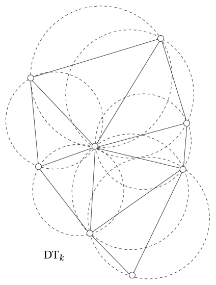
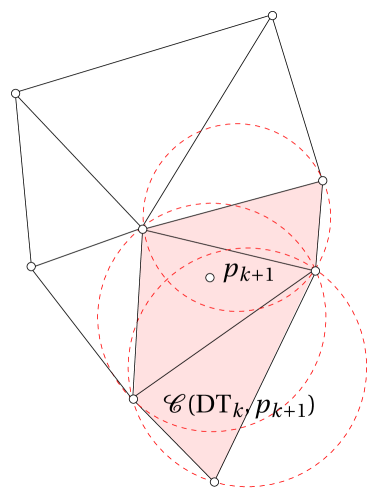
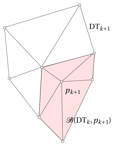
Fig. 2: Delaunay triangulation ${\mbox{DT}}_{k}$ (left), Delaunay cavity ${\mathcal{C}}_{p}({\mbox{DT}}_{k},{\mathbf{p}}_{k+1})$ (center) and ${\mbox{DT}}_{k+1}={\mbox{DT}}_{k}-{\mathcal{C}}({\mbox{DT}}_{k},{\mathbf{p}}_{k+1})+{\mathcal{B}}(\mbox{DT}_{k},\mathbf{p}_{k+1})$ (right).

Let ${\mbox{DT}}_{k}$ be the Delaunay triangulation of a point set $P_{k}=\{\mathbf{p}_{1},\dots,\mathbf{p}_{k}\}\subset\mathds{R}^{d}$. The Delaunay kernel is a procedure that allow the incremental insertion of a given point ${\mathbf{p}}_{k+1}\in\Omega(P_{k})$ into ${\mbox{DT}}_{k}$ and to build the Delaunay triangulation $\mbox{DT}_{k+1}$ of $P_{k+1}=\{\mathbf{p}_{1},\dots,\mathbf{p}_{k},\mathbf{p}_{k+1}\}.$ The Delaunay kernel can be written in the following abstract manner:

$${\mbox{DT}}_{k+1}={\mbox{DT}}_{k}-{\mathcal{C}}({\mbox{DT}}_{k},{\mathbf{p}}_{k+1})+{\mathcal{B}}(\mbox{DT}_{k},\mathbf{p}_{k+1}),$$ (4)

where the Delaunay cavity ${\mathcal{C}}({\mbox{DT}}_{k},{\mathbf{p}}_{k+1})$ is the set of all triangles whose circumcircles contain the new point $\mathbf{p}_{k+1}$ (see Figure 2; the triangles of the cavity cannot belong to ${\mbox{DT}}_{k+1}$) and the Delaunay ball ${\mathcal{B}}(\mbox{DT}_{k},\mathbf{p}_{k+1})$ is a set of triangles that fill the polyhedral hole that has been left empty while removing the Delaunay cavity ${\mathcal{C}}({\mbox{DT}}_{k},{\mathbf{p}}_{k+1})$ from $\mbox{DT}_{k}$.

It is possible to build ${\mbox{DT}}_{k+1}$ in ${\mathcal{O}}(n\log n)$ operations. The critical operation in the Delaunay kernel procedure is the construction of the cavity ${\mathcal{C}}({\mbox{DT}}_{k},{\mathbf{p}}_{k+1})$. A first element of the cavity $\tau$ is searched in $\mbox{DT}_{k}$ and the cavity is constructed using a depth first search algorithm that starts at $\tau$. Sorting the point set $P$ in such a way that two successive points in the set are close to each other geometrically allows to find $\tau$ in a number of operations that actually does not depend on $n$. We use her the standard BRIO sort that consist in sorting increasingly large subsets of $P$ along Hilbert curves. The points are not sorted all at once in order not to produce large cavities.

Building the cavity actually takes a number of operations that essentially depends on the dimension (2D or 3D). So, after the point set is sorted (${\mathcal{O}}(n\log n)$ operations), the insertion of the points takes ${\mathcal{O}}(n)$ operations.

It is possible to construct a multi-threaded version of the Delaunay kernel [19]. Assume $M$ computational threads that aim at inserting $M$ points in the triangulation at the same time. At the end, each thread is going to insert ${n\over M}$ points. The situation is of course not that simple: two points $\mathbf{p}_{i}$ and $\mathbf{p}_{j}$ can only be inserted at the same time in $\mbox{DT}_{k}$ if their respective Delaunay cavities ${\mathcal{C}}({\mbox{DT}}_{k},{\mathbf{p}}_{i})$ and ${\mathcal{C}}({\mbox{DT}}_{k},{\mathbf{p}}_{j})$ do not overlap, i.e., if they do not have triangles in common. A non-overlapping situation is more likely to happen if points $\mathbf{p}_{i}$ and $\mathbf{p}_{j}$ are not close geometrically. For that purpose, we split the Hilbert curve into $M$ equal parts and assign each part to one thread.

The multithreaded Delaunay kernel can be written in the following abstract manner:

$${\mbox{DT}}_{k+1}={\mbox{DT}}_{k}+\sum_{i=0}^{M-1}\left[{-\mathcal{C}}({\mbox{DT}}_{k},{\mathbf{p}}_{k+i{n\over M}})+{\mathcal{B}}(\mbox{DT}_{k},\mathbf{p}_{k+i{n\over M}})\right].$$ (5)

We have implemented the multithreaded Delaunay kernel using OpenMP [2]. Two OpenMP barriers were used at each iteration $k$. A first barrier is used after the computation of the $M$ cavities: every thread $i$ has to complete its cavity ${\mathcal{C}}({\mbox{DT}}_{k},{\mathbf{p}}_{k+i{n\over M}})$ at iteration $k$ in order to be able to verify that the cavity does not overlap other cavities. When several cavities overlap, only the point corresponding to the smallest thread number is processed. The other points are delayed to the next iteration. A second barrier is used after the construction of ${\mathcal{B}}(\mbox{DT}_{k},\mathbf{p}_{k+i{n\over M}})$: every thread has to finish computing the Delaunay kernel in order to start iteration $k+1$ with a valid mesh. This simple procedure usually produces speedups of $3$ on a quad-core computer. A two-level version of that procedure is now available in the 3D Delaunay mesher of Gmsh [6].

4 Building a valid 1D mesh

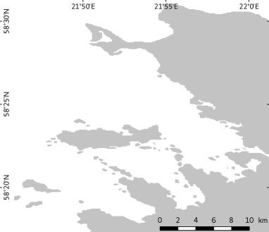
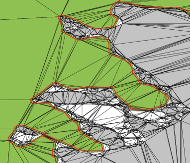
(a) high-resolution raw data	(b) and (c) generation of the coarse (1500m) geometry
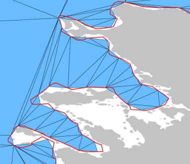
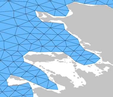
(d) discretization of the coarse geometry	(e) final mesh for a resolution of 1500m
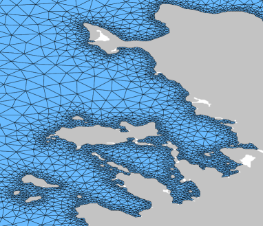
final mesh for a resolution of 750m along the coastlines	final mesh for a resolution of 150m along the coastlines

Fig. 3: Generation of a mesh coarser than the initial data.

The domain boundaries are extracted from geographical coastline databases. Due to their fractal nature, coastal shapes can be extremely complex and contain many small details. A major difficulty when dealing with coastline is that the resolution of the geographical database doest not match the desired mesh resolution. For example, the freely-available GSHHG [22] database has a maximal resolution bellow $100$m which is much too small for many numerical applications. In ocean modeling, a good practice would be that there exists no isolated island and no channel in the domain that are smaller than the mesh size. Small features should be removed from the description of the domain, eventually in an automatic fashion. If such small features exist, (i) badly shaped elements would be created in such channels or around those islands and (ii) the model will not be able anyway to capture relevant physics on features that are below mesh size.

Assume a mesh size field $h(x,y,z)$ that defines local sizes of mesh edges at point $x,y,z$ of the domain. We propose here a procedure that automatically creates a valid 1D mesh that: (i) does not overlap itself, (ii) contains no edges significantly smaller than $h$ and (iii) that defines the contour of a domain without water channels that are significantly narrower than $h$ (and in consequence, the boundary of the domain does no contain any angles that are strongly acute).

Figure 3 illustrates the different steps involved to build a coarse mesh from the high-resolution raw GSHHG data of the western coastline of the Saaremaa Island (Estonia) in the Baltic sea.

1. A high-resolution raw dataset is initially loaded. A mesh size field $h(x,y,z)$ is defined by the user. Any edge of the coastline data that is smaller than $h$ is refined.

2. A Delaunay mesh is built on the sphere with all the boundary points of the raw dataset. The user then selects one point $p$ that belongs to the region that has to be meshed. The unique curvilinear triangle $\tau$ that contains $p$ is then found by walking into the triangulation [4] and a depth-first search algorithm is applied to traverse the mesh, starting at root $\tau$. The algorithm stops whenever an edge smaller than $h$ is crossed (green triangles on sub-Figure (b) of Figure 3). This procedure defines a new set of edges that form a coarsened version of the domain that has no small features. Note here that the initial boundary of the domain cannot be traversed because edge size of the initial boundary is guaranteed to be smaller than $h$ (see point (a) above). Finally, note that the Delaunay mesh guarantees that two points closer to each other than $h$ in the initial triangulation will either be connected by an edge of the triangulation or connected by a series of edges smaller than $h$. This property prevents us to walk across narrow channels or across the original boundaries.

3. The external boundary of the green triangulation defines the new boundary of the domain of interest where all small features have been removed. At this point, the remaining isolated islands smaller than the prescribed mesh size are removed. There may exist edges inside the domain that are smaller than $h$. Such small edges are always bounded by two green triangles: they are embedded in the domain. To avoid this situation, which is problematic for the following steps, the whole boundary line (in red) is slightly (e.g. by $h/10$) shifted inside the domain.

4. The red line is the actual boundary of the domain. It is discretized with a prescribed mesh size. A Delaunay mesh is built with those points and the boundary edges are recovered by performing swaps.

5. Finally, a Delaunay refinement algorithm described below is applied to generate the points inside the domain.

A side benefit of this approach is that it requires only a mesh size field $h(x,y,z)$, the coordinates of one point inside the domain, and a series of (close) boundary points. In particular the initial boundary lines do not have to describe a correct topology. In other words, it is not a problem if two initial coastlines intersect each other. This makes it easy to mix various datasets or cut through a domain.

5 Multi-threaded Delaunay refinement

At that point, a valid 1D mesh has been produced. The following stage of the meshing algorithm consist in generating the surface mesh. For that, an “empty mesh” that contains all vertices of the 1D mesh is constructed on the sphere. Then, every edge of the 1D mesh that is not present in the empty mesh are recovered using edge swaps.

A Delaunay refinement procedure is applied to generate internal points of the domain. Here, we use an edge based approach. Every internal edge of the domain is “saturated” in the following way. Consider an edge ${\bf pq}$ of length $L=\|{\bf q}-{\bf p}\|$. A point ${\bf x}$ of ${\bf pq}$ has the form

$${\bf x}(u)={\bf p}(1-u)+{\bf q}u~{}~{},~{}~{}u\in[0,1].$$

The adimensional quantity

$$\rho(u)={L\over h({\bf x}(u))}$$

represents the mesh density at point ${\bf x}$ i.e. the number of points per unit of length that should be used to saturate an edge at point ${\bf x}$. The following primitive

$$\delta(t)=\int_{0}^{t}\rho(u)du$$

is very useful in what follows. We first note that $\delta(1)$ is the adimensional length of ${\bf pq}$. Its rounded up value $N=\lceil\delta(1)\rceil$ represents the number of subdivisions that is required to saturate edge ${\bf pq}$ i.e. to split ${\bf pq}$ with $N$ sub-segments that have an adimensional length close to one.

An adaptative trapezoidal integration scheme is used to compute $\delta(t)$ with a prescribed accuracy.

input : A mesh size field function $h({\bf x})$, an edge ${\bf pq}$ and a prescribed accuracy $\epsilon$.

output : A discrete representation of $\delta(t)=\int_{0}^{t}\rho(u)du$ as a list of $K$ points $(t_{j},\delta_{j})$, $j=1,\dots,K$.

Initialize a stack with one tuple $\{0,1,h({\bf x}(0)),h({\bf x}(1))\}$ with ${\bf x}(u)={\bf p}(1-u)+{\bf q}u.$;

Initialize an empty vector of tuples that contains the piecewise linear representation of the size field;

while stack is not empty do

       take tuple $\{u_{1},u_{2},h_{1},h_{2}\}$ at the top of the stack ;

       pop this tuple out of the stack ;

       compute $u_{12}=(u_{1}+u_{2})/2$ and $h_{12}=h({\bf x}(u_{12}))$;

      

      if  $\left|1/h_{12}-2/(h_{1}+h_{2})\right|>\epsilon\|{\bf p}-{\bf q}\|$  then

             push tuple $\{u_{12},u_{2},h_{12},h_{2}\}$ at the top of the stack;

            

            push tuple $\{t_{1},t_{12},h_{1},h_{12}\}$ at the top of the stack;

            

      else

             add tuple $\{u_{1},u_{2},h_{1},h_{2}\}$ to the result vector;

            

      

Algorithm 1 Adaptive trapezoidal rule that computes a piecewise linear representation of the size field along an edge ${\bf pq}$.

The primitive is numerically approximated by a piecewise linear function (see Algorithm 1). The $N-1$ points that form $N$ segments of adimensional size close to one on ${\bf pq}$ are situated at positions ${\bf x}(t_{j})$, $j=1,\dots,N-1$ with $t_{j}$ computed in such a way that

$$\delta(t_{j})=j{\delta(1)\over N}.$$

Points $t_{j}$ are computed using the piecewise approximation of $\delta(t)$.

At that point, it is interesting to give some justifications for that rather complex procedure. Mesh size functions $h({\bf x})$ can be complex functions involving heavy computations. In the cas of ocean modeling, $h$ may involve the distance to coastlines as well as local bathimetry . It is thus mandatory to minimize the number of function calls to $h$.

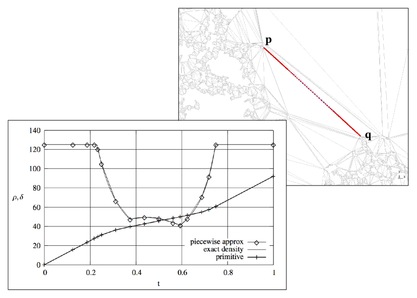
Fig. 4: Initial “empty mesh” of the baltic sea. Picture shows a zoom around an edge ${\bf pq}$. Points ${\bf x}_{j}$, $j=1,\dots,92$ that saturate the edge have been drawn in red. Computation of $\rho(t)$ and $\delta(t)$ on edge ${\bf pq}$ are shown as well. Only $K=16$ evaluations of $h({\bf x})$ were required to obtain a relative error of $5\%$ on $\rho$.

In order to illustrate that procedure, consider again the Baltic sea and a mesh size field

$$h({\bf x})=\left\{\begin{array}[]{lcl}h_{\min}&~{}~{}\mbox{if}{}{}&d({\bf x})<d_{\min}\\ h_{\min}+{d({\bf x})-d_{\min}\over d_{\max}-d_{\min}}(h_{\max}-h_{\min})&~{}~{}\mbox{if}{}{}&d_{\min}\leq d({\bf x})\leq d_{\max}\\ h_{\max}&~{}~{}\mbox{if}{}{}&d({\bf x})>d_{\max}\end{array}\right.$$ (6)

where $d({\bf x})$ is the distance to coastline (wall distance). The initial mesh (empty mesh) is depicted on Figure 4. On the same Figure, an edge ${\bf pq}$ is shown that has an adimensional length of $\delta(1)=92.12$ ($N=93$). Only $K=16$ points were necessary to represent $\rho$ with a prescribed accuracy of $\epsilon=5\%$. Both $\rho$ and $\delta$ are represented on Figure 4. The corresponding $92$ points ${\bf x}_{j}$ that saturate ${\bf pq}$ are plotted in red on the Figure as well.

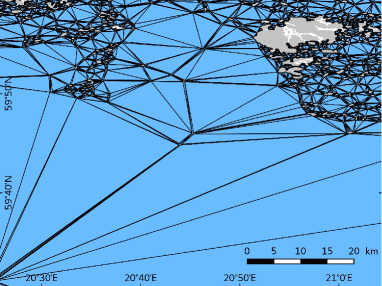
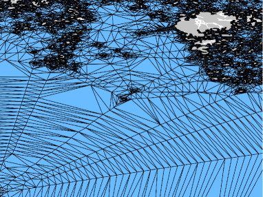
Triangulation of the 1D mesh	1 refinement step (471,312 points)
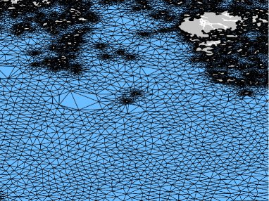
2 refinement steps (873,028 points)	3 refinement steps (969,283 points)
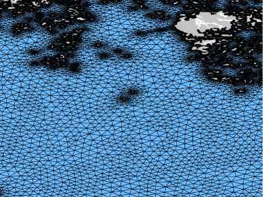
8 refinement steps (988,066 points)	8 refinement steps and smoothing

Fig. 5: Saturation of the edges. The final mesh (iteration 8) contains 2,345,823 triangles.

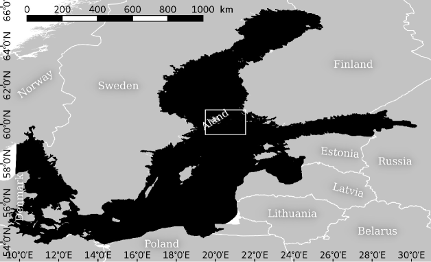
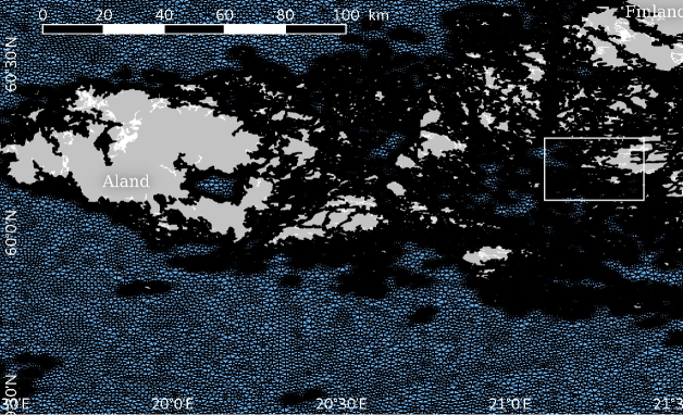
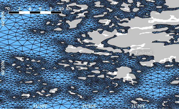
Fig. 6: Images of the final mesh of the Baltic sea.

At stage $i$ of the refinement process, all internal edges of the domain are saturated, producing a point set $P_{i}$. Points are spaced rightfully on edges of the existing mesh. Yet, there is no guarantee that points belonging to different edges are not too close to each other. Here, some filtering is required. Two approaches for filtering the points have been investigated. At first, a space search structure has been used (a RTree [1]). Using such a structure involves extra-storage. Insertions on a RTree in parallel is not an easy matter as well.

A more straightforward approach has been developed. The Delaunay kernel is applied to all points $p_{k}$ of $P_{j}$ without filtering. Consider triangulation ${\mbox{DT}}_{k-1}$ and the Delaunay cavity ${\mathcal{C}}({\mbox{DT}}_{k-1},{p}_{k})$ relative to point $p_{k}$ that has to be inserted in the mesh. There exist no points of ${\mbox{DT}}_{k-1}$ that are closer to $p_{k}$ than the points of ${\mathcal{C}}({\mbox{DT}}_{k-1},{p}_{k})$ thanks to the Delaunay property. Point $p_{k}$ is inserted if and only if no short edge is created during the insertion. It is thus only necessary to check points of the cavity in the filtering process.

In our implementation, both approaches have shown to provide similar serial performances. Yet, the approach based on the Delaunay kernel is clearly advantageous: (i) it is way easier to code (ceteris paribusis, a solution that is simpler to code is always better), (ii) it does not require any overhead and, (iii) more important, it enjoys the multi-threaded implementation of the Delaunay kernel.

Figure 5 illustrates the Delaunay refinement procedure on the Baltic sea. Final mesh of $2,345,823$ triangles has been generated in $16$ seconds on one thread. The size field function $h$ that has been chosen is highly computational intensive: The Delaunay kernel takes only $5,44$ seconds. Sorting the points along a 3D Hilbert curve takes $1,29$ seconds and saturating the edges takes $9,25$ seconds which is way more than half of the total CPU time. Note that parallelizing this stage of the algorithm is actually trivial. The algorithm converges when every edge has an adimensional length less or equal to oen. Eight iterations were necessary for convergence. Most of the points were inserted during the two first iterations (see Figure 5). Images of the final mesh are shown if Figure 6.

6 World ocean

In this section, we have generated a mesh of the whole world ocean with a global resolution of $h_{\min}=3$km. A larger mesh size of $h_{\min}=30$km was chosen far away from the coast like in Equation (6) (Figure 7). The final mesh contains 4,978,243 triangles and has been generated in about 50 seconds. About 30% of the total time was taken for generating the initial Delaunay mesh of the data. In the Delaunay refinement procedure 14.5 seconds were necessary to generate the points (saturation of the edges), 2.76 seconds were necessary to sort point sets $P_{j}$ and 8.44 seconds were used in the Delaunay kernel.

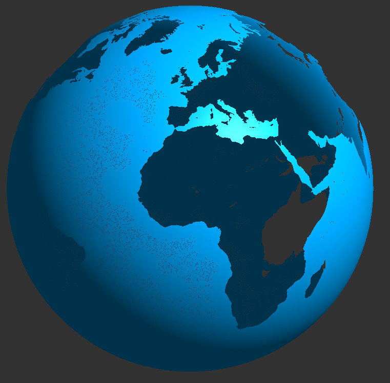
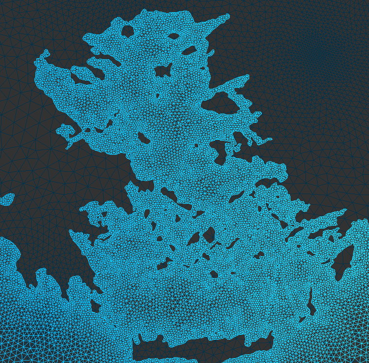
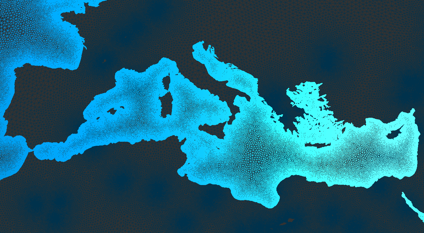
Fig. 7: Images of the mesh of the world ocean (top left) with a zoom on the Mediterranean sea (bottom) and on the Egean sea (top right).

7 Conclusions

This paper presents an original algorithm that allow to generate meshes of domains defined by coastline datas on the sphere. The main novelties of the approach are (i) the treatment of input data, (ii) the multithreaded nature of the algorithms and (iii) the Delaunay kernel on the sphere with automatic filtering. The extension to quadrilateral meshing is the following step in our developments.

The code that has been used here is a self consistent piece of code that will be released soon as an open source. It will be part of the Gmsh distribution.

Parallel computations will be presented in further communications.

References

- [1] N. Beckmann, H.-P. Kriegel, R. Schneider, and B. Seeger. The R*-tree: an efficient and robust access method for points and rectangles, volume 19. ACM, 1990.
- [2] L. Dagum and R. Menon. Openmp: an industry standard api for shared-memory programming. Computational Science & Engineering, IEEE, 5(1):46–55, 1998.
- [3] S. Danilov, G. Kivman, and J. Schröter. Evaluation of an eddy-permitting finite-element ocean model in the north atlantic. Ocean Modelling, 10:35–49, 2005.
- [4] O. Devillers, S. Pion, and M. Teillaud. Walking in a triangulation. International Journal of Foundations of Computer Science, 13(02):181–199, 2002.
- [5] P. L. George. Improvements on delaunay-based three-dimensional automatic mesh generator. Finite Elements in Analysis and Design, 25(3):297–317, 1997.
- [6] C. Geuzaine and J.-F. Remacle. Gmsh: A 3-d finite element mesh generator with built-in pre-and post-processing facilities. International Journal for Numerical Methods in Engineering, 79(11):1309–1331, 2009.
- [7] G. Gorman, M. Piggott, and C. Pain. Shoreline approximation for unstructured mesh generation. Computers and Geosciences, 33:666–677, 2007.
- [8] S. M. Griffies, C. Böning, F. O. Bryan, E. P. Chassignet, R. Gerdes, H. Hasumi, A. Hirst, A.-M. Treguier, and D. Webb. Developments in ocean climate modeling. Ocean Modelling, 2:123–192, 2000.
- [9] S. C. Hagen, J. J. Westerink, R. L. Kolar, and O. Horstmann. Two-dimensional, unstructured mesh generation for tidal models. International Journal for Numerical Methods in Fluids, 35:669–686, 2001. Printed version in Richard’s office.
- [10] R. F. Henry and R. A. Walters. Geometrically based, automatic generator for irregular triangular networks. Communications in numerical methods in engineering, 9:555–566, 1993.
- [11] J. Lambrechts, R. Comblen, V. Legat, C. Geuzaine, and J.-F. Remacle. Multiscale mesh generation on the sphere. Ocean Dynamics, 58(5-6):461–473, 2008.
- [12] J. Lambrechts, E. Hanert, E. Deleersnijder, P.-E. Bernard, V. Legat, J.-F. Remacle, and E. Wolanski. A multi-scale model of the hydrodynamics of the whole great barrier reef. Estuarine, Coastal and Shelf Science, 79(1):143–151, 2008.
- [13] C. Le Provost, M. L. Genco, and F. Lyard. Spectroscopy of the world ocean tides from a finite element hydrodynamic model. Journal of Geophysical Research, 99:777–797, 1994.
- [14] S. Legrand, E. Deleersnijder, E. Hanert, V. Legat, and E. Wolanski. High-resolution, unstructured meshes for hydrodynamic models of the great barrier reef, australia. Estuarine, Coastal and Shelf Science, 68:36–46, 2006.
- [15] S. Legrand, V. Legat, and E. Deleersnijder. Delaunay mesh generation for an unstructured-grid ocean circulation model. Ocean Modelling, 2:17–28, 2000.
- [16] F. Lyard, F. Lefevre, T. Letellier, and O. Francis. Modelling the global ocean tides: modern insights from FES2004. Ocean Dynamics, 56:394–415, 2006.
- [17] M. Piggott, G. Gorman, and C. Pain. Multi-scale ocean modelling with adaptive unstructured grids. CLIVAR Exchanges - Ocean model development and assessment, 12(42), 2007. http://eprints.soton.ac.uk/47576/.
- [18] D. QGis. Quantum gis geographic information system. Open Source Geospatial Foundation Project, 2011.
- [19] J.-F. Remacle, V. Bertrand, and C. Geuzaine. A two-level multithreaded delaunay kernel. Procedia Engineering, 124:6–17, 2015.
- [20] R. J. Renka. Algorithm 772: Stripack: Delaunay triangulation and voronoi diagram on the surface of a sphere. ACM Transactions on Mathematical Software (TOMS), 23(3):416–434, 1997.
- [21] M. G. Sassi, A. Hoitink, B. de Brye, B. Vermeulen, and E. Deleersnijder. Tidal impact on the division of river discharge over distributary channels in the mahakam delta. Ocean Dynamics, 61(12):2211–2228, 2011.
- [22] P. Wessel and W. Smith. Gshhg–a global self-consistent, hierarchical, high-resolution geography database. Honolulu, Hawaii, Silver Spring, Maryland.(URL: http://www. soest. hawaii. edu/pwessel/gshhg/(accessed 10 January2013), 2013.
- [23] L. White, E. Deleersnijder, and V. Legat. A three-dimensional unstructured mesh finite element shallow-water model, with application to the flows around an island and in a wind-driven elongated basin. Ocean Modelling, in press, 2008.