Reply to “Comment on Generalized Exclusion Processes: Transport Coefficients”

Abstract

We reply to the comment of Becker, Nelissen, Cleuren, Partoens, and Van den Broeck Com on our article we_14 about transport properties of a class of generalized exclusion processes.

Stochastic lattice gases with symmetric hopping are described, on a coarse-grained level, by diffusion equation with density-dependent diffusion coefficient. Density fluctuations additionally depend on the local conductivity (which also describes the response to an infinitesimal applied field). A hydrodynamic description therefore requires the determination of these two transport coefficients. Generally for lattice gases even with rather simple hopping rules, analytic results are unattainable; however, when an additional feature, known as the gradient condition, is satisfied, the Green-Kubo formula takes a simple form Spohn and computations of the transport coefficients become feasible. For a number of lattice gases of gradient type, e.g., for the Katz-Lebowitz-Spohn model with symmetric hopping KLS , for repulsion processes Krapivsky , for a lattice gas of leap-frogging particles CCGS ; GK , the diffusion coefficient has been rigorously computed. The gradient property is also true for the misanthrope process, a class of generalized exclusion processes C-T ; AM .

For gradient type lattice gases, an exact expression for the diffusion coefficient can also be obtained by a perturbation approach: one writes the formula for the current at the discrete lattice level and then performs a continuous limit assuming that the density field is slowly varying.

Generalized exclusion processes with multiple occupancies KLO94 ; KLO95 ; Timo ; BNCPV13 , in general, do not obey the gradient condition. However, we argued in we_14 that the perturbation approach should, nevertheless, lead to an exact prediction for the diffusion coefficient. For the class of generalized exclusion processes which we studied we_14 simulation results were indeed very close to the predictions by perturbative calculation. The comment Com by Becker et al. prompted us to perform more simulations and to analyze our results more carefully.

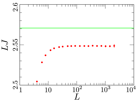
Figure 1: Stationary current multiplied by the system size: simulation results (dots) and the prediction from our previous approach. The latter holds for $L=\infty$, but is shown as a line.

Becker et al. computed numerically the diffusion coefficient $D(\rho)$. They performed simulations for various system sizes $L$ and various density differences $\delta\rho$ between the boundary reservoirs. In order to extract $D(\rho)$ from simulations they needed to take Com two limits: $L\to\infty$ and $\delta\rho\to 0$. We considered a system with a large density difference and measured the stationary current through the system: the advantage is that we have to take only one limit, $L\to\infty$. We analyzed the generalized exclusion process GEP(2) with maximal occupancy $k=2$ particles per site and extreme densities at the boundaries: $\rho(0)=2$ and $\rho(L)=0$. According to our expectations we_14 , the average current should vanish as $(1+\frac{\pi}{2})/L$ when $L\gg 1$. Simulation results (Fig. 1) demonstrate that the error is smaller than $0.9\%$, but this discrepancy does not seem to disappear in the $L\to\infty$ limit.

The numerical results of Ref. Com and our simulations (Fig. 1) show that the perturbation approach does not lead to the correct analytical results for the GEP(2). We emphasize that the perturbation approach is not a naive mean-field theory where correlations are obviously neglected as argued by Becker et al. In dense lattice gases, the equilibrium state itself is usually highly correlated; e.g., in the repulsion process $\langle\tau_{i}\tau_{i+1}\rangle=0\neq\rho^{2}$ for $0\leq\rho\leq\frac{1}{2}$, where $\tau_{i}\in\{1,0\}$ denotes the occupation number of site $i$: the mean-field assumption is completely wrong. Yet, a careful use of the perturbation approach leads to the correct result Krapivsky .

The gradient condition is thus crucial for the applicability of the perturbation approach. For GEP($k$) with maximal occupancy $k$, the gradient condition is obeyed in extreme cases of $k=1$ which reduces to the simple exclusion process and $k=\infty$ which reduces to random walks. Presumably because GEP($k$) is sandwiched between two extreme cases in which the perturbation approach works, this method provides a very good approximation when $1<k<\infty$.

We now clarify the underlying assumptions behind the perturbation approach and suggest some tracks to improve our results. For the GEP(2), the current reads

$$J_{i}=\langle\tau_{i}f(\tau_{i+1})-f(\tau_{i})\tau_{i+1}\rangle,$$ (1)

where $\tau_{i}\in\{0,1,2\}$ and $f(n)=1-\frac{1}{2}n(n-1)$. In our computation of the diffusion coefficient we_14 , we used two assumptions. The first one concerns one-point functions. Let $\mathbb{P}[\tau_{i}=m]$ be the probability of finding $m$ particles at site $i$. The density at $i$ is

$$\rho_{i}=\langle\tau_{i}\rangle=\mathbb{P}[\tau_{i}=1]+2\mathbb{P}[\tau_{i}=2].$$ (2)

We assumed that one-site probabilities satisfy

$$\mathbb{P}[\tau_{i}=m]\simeq X_{m}(\rho_{i})\quad$$ (3)

where the $X_{m}$’s represent the single-site weights in an infinite lattice or on a ring:

$$X_{0}(\rho)=\frac{1}{Z},\ X_{1}(\rho)=\frac{\lambda}{Z},\ X_{2}(\rho)=\frac{\lambda^{2}}{2Z}$$ (4)

with the fugacity $\lambda$ and the normalization $Z$

$$\lambda(\rho)=\frac{\sqrt{1+2\rho-\rho^{2}}+\rho-1}{2-\rho},\ Z=1+\lambda+\frac{1}{2}\lambda^{2}.$$ (5)

The second assumption was to rewrite the current as

$$J_{i}\simeq\langle\tau_{i}\rangle\langle f(\tau_{i+1})\rangle-\langle f(\tau_{i})\rangle\langle\tau_{i+1}\rangle.$$ (6)

This, indeed, is a mean-field type assumption Com . The assumptions (3), (6) are asymptotically true in the stationary state of a large system ($L\to\infty$): We have checked these facts by performing additional simulations.

Our numerical results suggest more precise expressions for (3) and (6) with some scaling functions $\kappa$ and $\mu$:

$$\mathbb{P}[\tau_{i}=m]=X_{m}(\rho_{i})+\frac{1}{L}\kappa_{m}\Big{(}\frac{i}{L}\Big{)}\,,$$ (7)

$$J_{i}=\langle\tau_{i}\rangle\langle f(\tau_{i+1})\rangle-\langle f(\tau_{i})\rangle\langle\tau_{i+1}\rangle+\frac{1}{L}\mu\Big{(}\frac{i}{L}\Big{)},$$ (8)

where we omitted $o(L^{-1})$ terms. Performing the perturbation approach with the refined expressions (7), (8), we obtain

$$J=-\frac{1}{L}\frac{d\rho}{dx}\left(1-X_{2}(\rho)+\rho\frac{dX_{2}(\rho)}{d\rho}\right)+\frac{1}{L}\mu(x)$$ (9)

where we have switched from the discrete variable $i$ to $x=i/L$. The functions $\kappa_{m}$ do not appear in (9), but $\mu(x)$ does, and it was missing in our paper we_14 leading to the wrong expressions for the current and for the stationary density profile. In order to calculate $\mu(x)$, we are presently examining nearest-neighbor correlation functions for the GEP(2). Numerically at least, these nearest-neighbor correlations exhibit a neat scaling behavior and simple patterns; detailed results will be reported in we_future .

References

- (1) T. Becker, K. Nelissen, B. Cleuren, B. Partoens, and C. Van den Broeck, Phys. Rev. E 93, 046101 (2016).
- (2) C. Arita, P. L. Krapivsky, and K. Mallick, Phys. Rev. E 90, 052108 (2014).
- (3) H. Spohn, Large Scale Dynamics of Interacting Particles (New York: Springer-Verlag, 1991).
- (4) S. Katz, J. L. Lebowitz, and H. Spohn, J. Stat. Phys. 34, 497 (1984).
- (5) P. L. Krapivsky, J. Stat. Mech. P06012 (2013).
- (6) J. M. Carlson, J. T. Chayes, E. R. Grannan, and G. H. Swindle, Phys. Rev. Lett. 65, 2547 (1990).
- (7) D. Gabrielli and P. L. Krapivsky, in preparation.
- (8) C. Cocozza-Thivent, Z. Wahrscheinlichkeitstheorie verw. Gebiete 70, 509 (1985).
- (9) C. Arita and C. Matsui, arXiv:1605.00917.
- (10) C. Kipnis, C. Landim, and S. Olla, Commun. Pure Appl. Math. 47, 1475 (1994).
- (11) C. Kipnis, C. Landim, and S. Olla, Ann. Inst. H. Poincaré 31, 191 (1995).
- (12) T. Seppäläinen, Ann. Prob. 27, 361 (1999).
- (13) T. Becker, K. Nelissen, B. Cleuren, B. Partoens, and C. Van den Broeck, Phys. Rev. Lett. 111, 110601 (2013).
- (14) C. Arita, P. L. Krapivsky, and K. Mallick, in preparation.