Detection of periodicity in functional time series

Abstract

We derive several tests for the presence of a periodic component in a time series of functions. We consider both the traditional setting in which the periodic functional signal is contaminated by functional white noise, and a more general setting of a contaminating process which is weakly dependent. Several forms of the periodic component are considered. Our tests are motivated by the likelihood principle and fall into two broad categories, which we term multivariate and fully functional. Overall, for the functional series that motivate this research, the fully functional tests exhibit a superior balance of size and power. Asymptotic null distributions of all tests are derived and their consistency is established. Their finite sample performance is examined and compared by numerical studies and application to pollution data.

¹ Department of Mathematics, Université libre de Bruxelles CP210, Bd. du Triomphe, B-1050 Brussels, Belgium.

² Department of Statistics, Colorado State University, Fort Collins, CO 80523-1877, USA.

³ ECARES, Université libre de Bruxelles, 50 Avenue Franklin Roosevelt, B-1050 Brussels, Belgium.

MSC 2010 subject classifications: Primary 62M15, 62G10; secondary 60G15, 62G20
Keywords: functional data, time series data, periodicity, spectral analysis, testing, asymptotics.

1 Introduction

Periodicity is one of the most important characteristics of time series, and tests for periodicity go back to the very origins of the field, e.g. [1898], [1914], [1929], [1957], [1961], among many others. An excellent account of these early developments is given in Chapter 10 of [1991].

We respond to the need to develop periodicity tests for time series of functions—short functional time series (FTS’s). Examples of FTS’s include annual temperature or smoothed precipitation curves, e.g. [2016], daily pollution level curves, e.g. [Aue et al. (2015)], various daily curves derived from high frequency asset price data, e.g. [2014], yield curves, e.g. [2012], daily vehicle traffic curves, e.g. [2016]. More complex objects, like sequences of 2D satellite images or 3D brain scans, have also been considered, e.g. [2008] and [2007], but the FDA methodology for such time series of complex data objects is still under development. Our theory covers such series, but the numerical implementation we developed currently applies only to functions defined on an interval.

This work is motivated both by the need to address a general inferential problem and by specific data with which we have worked over the past decade. We first discuss the general motivation, then we illustrate it using the data.

Most inferential procedures for FTS’s require that the series be stationary (several examples for such procedures can be found in [2012]). However, pollution levels, finance or traffic data may exhibit periodic (e.g. weekly) patterns, and then the stationarity assumption is violated. [2014] propose several testing procedures from the so-called KPSS family to test the stationarity of an FTS. Their approach is based on functionals of a CUSUM process, which makes it powerful when testing against changes in the mean or against integration of order 1. However, it is not designed for testing against a periodic signal. Finding periodicity in a data set is also of direct relevance for understanding the problem at hand as will be illustrated in Section 6. Exploiting the full information contained in the shapes of functions is crucial. Tests of periodicity for FTS’s can be applied to the observed functions or to residual functions obtained after fitting some model. If periodicity is found in the residuals, it may indicate an inadequate model fit.

Figure 1: Boxplots of PM10 (left) and NO (right) for each to day of the week. The sample consists of $N$=167 days.

The following motivating example, which is described in detail in Section 6, illustrates the need to develop new tests that exploit the functional structure of the data. Figure 1 shows boxplots of daily averages of the pollutants PM10 (fine dust) and NO (nitrogen monoxide) measured in Graz, Austria during the winter season 2015/16. The boxplots are grouped by weekdays and we want to infer if the corresponding group means differ significantly. Due to the traffic exposure of the measuring device in the city center and the weekday dependent traffic volumes reported in [2004], significant differences between the groups are expected. But although the boxplots indicate lower concentrations on Sundays, the variation within the groups is relatively large, and from a one-way ANOVA we do not obtain evidence against the null hypothesis of equal weekday means. The $p$-values are $0.75$ (PM10) and $0.27$ (NO), respectively. It needs to be stressed at this point, that formally ANOVA is not theoretically justified since we are analyzing time series data which are serially correlated. Nevertheless, we will see in Section 6 that for both data sets the conclusion remains the same even after adjusting the test for dependence. Now let us look at this problem from a functional data perspective. Figure 2 shows intraday mean curves (our raw pollution data are available up to half-hour resolution) of both pollutants during the same winter season. The plot suggests that Saturday and Sunday mean curves differ from those of working days. While they have smaller peaks, they have higher lows (presumably due to lower commuter traffic and higher nighttime activity on weekends). The methodology developed in the subsequent sections, will allow us to judge whether the differences in the functional means are significant. In this particular example the answer is confirmative. Hence, in contrast to daily averages, the intraday mean functions do significantly depend on the day of the week.

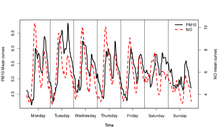
Figure 2: Weekday means of PM10 (solid black) and NO (red dashed).

One of the important contributions of this paper is the development of a fully functional ANOVA test for dependent data. Using a frequency domain approach, we obtain the asymptotic null distribution of the functional ANOVA statistic. This result is formulated in Corollary 4.1. The limiting distribution has an interesting form and can be written as a sum of independent hypoexponential variables whose parameters are eigenvalues of the spectral density operator of $(Y_{t})$. To the best of our knowledge, there exists no comparable asymptotic result in FDA literature.

Adapting ANOVA for stationary time series is one way to conduct periodicity analysis. It is suitable when the periodic component has no particular form. If, however, the alternative is more specific, then we can construct simpler and more powerful tests. In Section 2, we introduce three different models of increasing complexity, and in Section 3 we develop the appropriate test statistics. By considering specific local alternatives the power advantage will be numerically illustrated in Section 8 and theoretical supported in the supplemental material (Appendix E). General consistency results are provided in Section 5.

We have emphasized so far fully functional testing procedures which are theoretically elegant and appealing. A common approach to inference for functional data is to project observations onto a low dimensional basis system and then to apply a suitable multivariate procedure to the vector of projections. This approach will be outlined in Section 3.1. Our multivariate results improve upon [1974] in two ways: First, our tests are derived from a (Gaussian) likelihood-ratio approach. As we will see, this provides a power advantage over MacNeill’s test. Second, we extend all our tests in Section 4 to a very general weak dependence setting, as opposed to linear processes studied in [1974] and [1961].

Our methodology and theory for dependent FTS’ are based on new developments in the Fourier methods for such series. The work of Panaretos and Tavakoli (?, ?) introduces the main concepts of this approach, such as the functional periodogram and spectral density operators. This framework has been recently extended and used in other contexts, see e.g. [2015] and [2016]. [2016] use it in a setting that falls between our models (2.3) and (2.6) (iid Gaussian error functions), which also allows them to derive tests for hidden periodicities; the climate data they study may exhibit some a priori unspecified periods. For the data that motivate our work (pollution, traffic, temperature, economic and and finance data), the potential period is known (week, year, etc.), and they generally exhibit dependence under the null. This work therefore focuses on a fixed known period and weakly dependent functions.

The remainder of the paper is organized as follows. In Sections 2 and 3, we consider models and tests under the null of iid Gaussian functions. Section 4 considers dependent non–Gaussian functions. Consistency of the tests is established in Section 5. Applications to pollution data and a simulation study are presented, respectively, in Sections 6 and 7. In Section 8, we numerically assess asymptotic local power of the tests. The main contributions and findings are summarized in Section 9. All technical results and proofs that are not necessary to understand and apply the new methodology are presented in the supplemental material.

2 Models for periodic functional time series

The classical model, [1929], for a (scalar) periodic signal contaminated by noise is

(2.1) $$y_{t}=\mu+\alpha\cos(t\theta)+\beta\sin(t\theta)+z_{t},$$

where the $z_{t}$ are normal white noise, $\alpha$, $\beta$ and $\mu$ are unknown constants and $\theta\in[-\pi,\pi]$ is a known frequency which determines the period. Model (2.1) has been extended in several directions, for example, by replacing a pure harmonic wave by an arbitrary periodic component and/or by replacing the normal white noise by a more general stationary time series, as well as by considering multivariate series.

In this section, we list extensions to functional time series organizing them by increasing complexity. Our theory is valid in an arbitrary separable Hilbert space $H$, in which $\langle x,y\rangle$ denotes the inner product and $\|x\|=\sqrt{\langle x,x\rangle}$ the corresponding norm, $x,y\in H$. In most applications, it is the space $L^{2}$ of square integrable functions on a compact interval, in which case $\langle x,y\rangle=\int x(u)y(u)du$. A comprehensive exposition of Hilbert space theory for functional data is given in [2015].

We begin by stating the following (preliminary) assumption on the functional noise process.

Assumption 2.1.

The noise $(Z_{t})$ is an i.i.d. sequence in $H$, with each $Z_{t}$ being a Gaussian element in $H$ with zero mean and covariance operator $\Gamma$.

Recall that a random variable $Z$ in $H$ is Gaussian, in short $Z\sim\mathcal{N}_{H}(\mu,\Gamma)$, if and only if all projections $\langle Z,v\rangle$, $v\in H$, are normally distributed with mean $\langle\mu,v\rangle$ and variance $\langle\Gamma(v),v\rangle$. Working under Assumption 2.1 is convenient because we can motivate our tests proposed in Section 3 by a likelihood ratio approach and calculate exact distributions. Nevertheless, this framework is too restrictive for many applied problems. We devote Section 4 to procedures applicable in case of noise which is a general stationary functional time series. The testing problems remain the same, but the test statistics and/or critical values change.

To make the exposition more specific and focused on the main ideas, we introduce the following assumption.

Assumption 2.2.

The sample size $N$ is a multiple of the period, $N=dn$, where the period $d>1$ is odd. We set $q=(d-1)/2$.

Appendix A discusses modifications needed in case of even $d$. Assuming that the sample size $N$ is a multiple of $d$ is not really restrictive and can easily be achieved by trimming up to $d-1$ data points.

The simplest extension of model (2.1) to a functional setting is

(M.1) $$Y_{t}(u)=\mu(u)+[\alpha\cos(t\theta)+\beta\sin(t\theta)]w(u)+Z_{t}(u),\quad\mu,\,w\in H,\quad\alpha,\beta\in\mathbb{R}.$$

If $\rho:=\sqrt{\alpha^{2}+\beta^{2}}=0$, then $(Y_{t}\colon t\geq 1)$ is functional Gaussian white noise with a mean function $\mu$. If $\rho>0$, then a periodic pattern is added, which varies along the direction of a function $w$. To ensure identifiability, we assume that $\|w\|^{2}:=\int_{0}^{1}w^{2}(u)du=1$. The functions $\mu$ and $w$, as well as the parameters $\alpha$ and $\beta$ are assumed to be unknown. As explained in the Introduction, the parameter $\theta$, which determines the period $d$, is assumed to be a known positive fundamental frequency, i.e

$$\theta\in\Theta_{N}:=\left\{\theta_{j}=2\pi j/N,\;j=1,\ldots,m:=\left[(N-1)/2\right]\right\}.$$

The testing problem is

(2.2) $$\mathcal{H}_{0}\colon\rho=0\ \ \ {\rm vs.}\ \ \ \mathcal{H}_{A}\colon\rho>0.$$

A first extension of (M.1) is to replace $\alpha\cos(\theta t)+\beta\sin(\theta t)$ by some arbitrary $d$–periodic sequence. A more general model thus is

(M.2) $$Y_{t}(u)=\mu(u)+s_{t}w(u)+Z_{t}(u),\quad s_{t}=s_{t+d},\ \ \ \mu,w\in H.$$

We wish to test

(2.3) $$\mathcal{H}_{0}\colon s_{1}=s_{2}=\cdots=s_{d}=0\quad\text{against}\quad\mathcal{H}_{A}\colon\max_{1\leq t\leq d}|s_{t}|>0.$$

Here we impose the identifiability constraints $\|w\|=1$ and $\sum_{k=1}^{d}s_{t}=0$. The latter ensures that the vector $(s_{1},\ldots,s_{d})^{\prime}$ is contained in the subspace spanned by the orthogonal vectors

$$\begin{pmatrix}\cos(\theta_{n})\\ \cos(2\theta_{n})\\ \vdots\\ \cos(d\theta_{n})\end{pmatrix},\begin{pmatrix}\sin(\theta_{n})\\ \sin(2\theta_{n})\\ \vdots\\ \sin(d\theta_{n})\end{pmatrix},\ldots,\begin{pmatrix}\cos(\theta_{nq})\\ \cos(2\theta_{nq})\\ \vdots\\ \cos(d\theta_{nq})\end{pmatrix},\begin{pmatrix}\sin(\theta_{nq})\\ \sin(2\theta_{nq})\\ \vdots\\ \sin(d\theta_{nq})\end{pmatrix},$$

cf. Assumption 2.2. With the convention

(2.4) $$\vartheta_{k}:=\theta_{nk}=2\pi k/d,$$

model (M.2) can be written as

(2.5) $$Y_{t}(u)=\mu(u)+\left(\sum_{k=1}^{q}\big{(}\alpha_{k}\cos(t\vartheta_{k})+\beta_{k}\sin(t\vartheta_{k})\big{)}\right)w(u)+Z_{t}(u),$$

with some coefficients $\alpha_{k}$ and $\beta_{k}$.

Model (M.2) assumes that at any point of time, the periodic functional component is proportional to a single function $w$. A model which imposes periodicity in a very general sense is

(M.3) $$Y_{t}(u)=\mu(u)+w_{t}(u)+Z_{t}(u),\quad\mu,w_{t}\in H,\quad w_{t}=w_{t+d},\quad\sum_{t=1}^{d}w_{t}=0.$$

In this context, we test

(2.6) $$\mathcal{H}_{0}\colon w_{1}=w_{2}=\cdots=w_{d}=0\quad\text{against}\quad\mathcal{H}_{A}\colon\max_{1\leq t\leq d}\|w_{t}\|>0.$$

Model (M.3) contains models (M.1) and (M.2) as special cases. Under $\mathcal{H}_{0}$ all three models are identical. Test procedures presented in Section 3 are motivated by specific models as they point toward specific alternatives. However, they can be applied to any data, and, as we demostrate in Sections 6 and 7, tests motivated by simple models often perform very well for more complex alternatives.

3 Test procedures in presence of Gaussian noise

In the following subsections, we present the basic form of periodicity tests. Throughout this section, we work under Assumptions 2.1 and 2.2. In Section 4 and Appendix A, respectively, we show how to remove these assumptions. Details of mathematical derivations are given in Appendix B.

Let us start by introducing the necessary notation and notational conventions. Given a vector time series $(\bm{Y}_{t}\colon 1\leq t\leq N)$ the discrete Fourier transform (DFT) is $\bm{D}(\theta)=\frac{1}{\sqrt{N}}\sum_{k=1}^{N}\bm{Y}_{k}e^{-\mathrm{i}k\theta}$, $\theta\in[-\pi,\pi]$. We will use the decomposition into real and complex parts: $\bm{D}(\theta)=\bm{R}(\theta)+\mathrm{i}\bm{C}(\theta)$. At some places we may add a subscript to indicate the dependence on the sample size and/or a superscript to refer to the underlying data. (E.g. $\bm{R}_{N}^{\bm{Y}}(\theta)$.) We proceed analogously for a functional time series $(Y_{t}\colon 1\leq t\leq N)$. Then the DFT is denoted by $D(\theta)=R(\theta)+\mathrm{i}C(\theta)$.

Let us set $\bm{A}(\theta_{i_{1}},\ldots,\theta_{i_{k}})=\big{[}\bm{R}(\theta_{i_{1}}),\ldots,\bm{R}(\theta_{i_{k}}),\bm{C}(\theta_{i_{1}}),\ldots,\bm{C}(\theta_{i_{k}})\big{]}^{\prime}$ and analogously $A(\theta_{i_{1}},\ldots,\theta_{i_{k}})$ be a $2k$-vector of functions with components $R(\theta_{i_{j}})$ and $C(\theta_{i_{j}})$. If $A=(A_{1},\ldots,A_{k})^{\prime}$ is any $k$-vector of functions, then $AA^{\prime}$ is the $k\times k$ matrix of scalar products $\langle A_{i},A_{j}\rangle$. We use $\|M\|$ for the usual (Euclidean) norm and $\|M\|_{\mathrm{tr}}$ for the trace norm of some generic matrix $M$. Finally, $\mathbf{W}_{p}(n)$ denotes the real $p\times p$ Wishart matrix with $n$ degrees of freedom and $q_{\alpha}(X)$ is the $\alpha$-quantile of some variable $X$.

3.1 Projection based approaches

Typically functional data are represented in a smoothed form by finite dimensional systems, such as B–splines, Fourier basis, wavelets, etc. Additional dimension reduction can be achieved by functional principal components or similar data–driven systems. It is thus natural to search for a periodic pattern within a lower dimensional approximation of the data.

In this section, we assume that $v_{1},v_{2},\ldots,v_{p}$ is a suitably chosen set of linearly independent functions. Setting $\bm{Y}_{t}:=(\langle Y_{t},v_{1}\rangle,\ldots,\langle Y_{t},v_{p}\rangle)^{\prime}$, we obtain vector observations. Under $\mathcal{H}_{0}$, the time series $(\bm{Y}_{t})$ is i.i.d. Gaussian with covariance matrix $\bm{\Sigma}=(\langle\Gamma(v_{i}),v_{j}\rangle\colon 1\leq i,j\leq p)$. Under $\mathcal{H}_{A}$ we can write the projected version of model (M.3) as

(3.1) $$\bm{Y}_{t}=\bm{\mu}+\bm{w}_{t}+\bm{Z}_{t},$$

with $\bm{\mu}=(\langle\mu,v_{1}\rangle\cdots\langle\mu,v_{p}\rangle)^{\prime}$, $\bm{w}_{t}=(\langle w_{t},v_{1}\rangle\cdots\langle w_{t},v_{p}\rangle)^{\prime}$ and the innovations $\bm{Z}_{t}=(\langle Z_{t},v_{1}\rangle\cdots\langle Z_{t},v_{p}\rangle)^{\prime}$. This in turn can be specialized to projected versions of models (M.1) and (M.2). Provided the periodic component in the investigated model is not orthogonal to  $\mathrm{span}\{v_{1},v_{2},\ldots,v_{p}\}$, we can formulate the corresponding multivariate testing problems. In the following theorem we state the likelihood ratio tests. Recall the definition of the frequencies $\vartheta_{k}$ in (2.4) and the notation $q=(d-1)/2$.

Theorem 3.1.

For a given positive definite $\bm{\Sigma}$, the likelihood-ratio tests for the multivariate analogues of testing problems (2.2), (2.3) and (2.6) (related to the projected models (M.1), (M.2) and (M.3), respectively) are given as follows: Reject the null-hypothesis at level $\alpha$ if

$$T^{{\tt MEV}_{1}} :=\big{\|}\bm{A}(\vartheta_{1})\bm{\Sigma}^{-1}\bm{A}^{\prime}(\vartheta_{1})\big{\|}>q_{1-\alpha}[\|\mathbf{W}_{p}(2)\|/2];$$

$$T^{{\tt MEV}_{2}} :=\big{\|}\bm{A}(\vartheta_{1},\ldots,\vartheta_{q})\bm{\Sigma}^{-1}\bm{A}^{\prime}(\vartheta_{1},\ldots,\vartheta_{q})\big{\|}>q_{1-\alpha}[\|\mathbf{W}_{p}(d-1)\|/2];$$

$$T^{{\tt MTR_{2}}} :=\big{\|}\bm{A}(\vartheta_{1},\ldots,\vartheta_{q})\bm{\Sigma}^{-1}\bm{A}^{\prime}(\vartheta_{1},\ldots,\vartheta_{q})\big{\|}_{\mathrm{tr}}>q_{1-\alpha}[\mathrm{Erlang}(pq,1)].$$

Some remarks are in order.

1. The superscript MEV in our tests stands for Multivariate EigenValue. Multivariate, as opposed to functional, and eigenvalue, refers to the fact that the Euclidean matrix norm of a symmetric matrix is equal to its largest eigenvalue. MTR abbreviates Multivariate TRace.

2. By Lemma B.1, the columns of $\bm{\Sigma}^{-1/2}\bm{A}^{\prime}(\vartheta_{1},\ldots,\vartheta_{q})$ are i.i.d. $\mathcal{N}_{p}(0,\frac{1}{2}I_{p})$. This explains the Wishart distribution. For explicit computation of the quantiles $q_{1-\alpha}[\|\mathbf{W}_{p}(k)\|]$ we refer to [2014].

3. An alternative to the test based on $T^{{\tt MEV}_{1}}$ is

   $$T^{{\tt MTR}_{1}}=\big{\|}\bm{A}(\vartheta_{1})\bm{\Sigma}^{-1}\bm{A}^{\prime}(\vartheta_{1})\big{\|}_{\mathrm{tr}}>q_{1-\alpha}[\mathrm{Erlang}(p,1)].$$

   The latter can be seen to be equivalent to the test proposed by [1974] for a multivariate version of model (M.1). The likelihood ratio and MacNeill’s test statistic are related to different matrix norms of $\bm{A}(\vartheta_{1})\bm{\Sigma}^{-1}\bm{A}^{\prime}(\vartheta_{1})$. By the Neyman–Pearson lemma, a likelihood ratio test, even in an approximate form, can be expected to have good and sometimes even optimal power properties. Likewise, replacing the matrix norm in $T^{{\tt MEV}_{2}}$ by the trace norm leads to $T^{{\tt MTR_{2}}}$. As Figure 3 illustrates, the difference in power between the two tests can be quite noticeable, especially when $d$ is large.

4. In practice, $\bm{\Sigma}$ must be replaced by a consistent estimator. The construction of such estimators, which remain consistent under $\mathcal{H}_{A}$, is discussed in Appendix D.

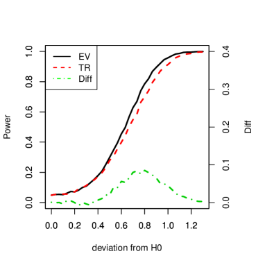
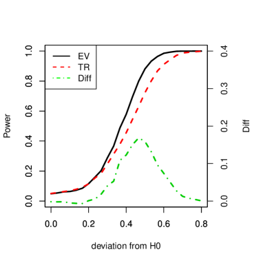
Figure 3: Local asymptotic power curves of tests $T^{{\tt MEV}_{2}}$ (EV) and $T^{{\tt MTR_{2}}}$ (TR), and their difference (Diff, right scale). Left panel: $p=5$ and $d=7$, right panel: $p=5$ and $d=31$. Details of the implementation are given in Section 8.

3.2 Fully functional tests

The projection based approaches of the previous section may be sensitive to the choice of the basis and to the number of basis functions. It is hence desirable to develop some fully functional procedures to bypass this problem. Before we introduce fully functional test statistics, let us observe that $T^{\tt MEV_{i}}$ and $T^{\tt MTR_{i}}$ $(i=1,2)$ are computed from the rescaled sample $\mathbf{\Sigma}^{-1/2}\bm{Y}_{1},\ldots,\mathbf{\Sigma}^{-1/2}\bm{Y}_{N}$, which results in asymptotically pivotal tests. The rescaling guarantees that the component processes with larger variation are not concealing potential periodic patterns in components with little variance. While this is clearly a very desirable property in multivariate analysis, one may favor a different perspective for functional data. If $\bm{Y}_{t}$ are principal component scores, then $\mathbf{\Sigma}=\mathrm{diag}(\lambda_{1},\ldots,\lambda_{p})$, where $\lambda_{i}$ are the eigenvalues of $\mathrm{Cov}(Z_{1})$. Suppose that $Y_{t}(u)=\sqrt{\lambda_{\ell}}\cos(2\pi t/d)v_{\ell}(u)+Z_{t}(u)$, $\ell\geq 1$. Then, due to $\lambda_{\ell}\to 0$, the bigger $\ell$, the smaller and more negligible the periodic signal is. However, it is easily seen that for any of our multivariate tests, the probability of rejecting $\mathcal{H}_{0}$ is the same for all values $1\leq\ell\leq p$.

A way to account for the functional nature of the data is to base the test statistics directly on the unscaled and fully functional observations, i.e. to define analogues of the test statistics in Theorem 3.1 with the matrices $A(\vartheta_{1})A^{\prime}(\vartheta_{1})$ (in $\mathbb{R}^{2\times 2}$) and $A(\vartheta_{1},\ldots,\vartheta_{q})A^{\prime}(\vartheta_{1},\ldots,\vartheta_{q})$ (in $\mathbb{R}^{(d-1)\times(d-1)}$). Since, to the best of our knowledge, there is no result available on the distribution of $\big{\|}A(\vartheta_{1},\ldots,\vartheta_{q})A^{\prime}(\vartheta_{1},\ldots,\vartheta_{q})\big{\|}$, we shall only consider the trace norm for which we can get explicit formulas. Hence, for model (M.1) we propose a test which rejects $\mathcal{H}_{0}$ at level $\alpha$ if

$$T^{{\tt FTR_{1}}}:=\|A(\vartheta_{1})A^{\prime}(\vartheta_{1})\|_{\mathrm{tr}}>q_{1-\alpha}[\mathrm{HExp}(\lambda_{1},\lambda_{2},\ldots)].$$

Here $\mathrm{HExp}(\lambda_{1},\lambda_{2},\ldots)$ denotes a random variable which is distributed as $\sum_{i\geq 1}\lambda_{i}E_{i}$, where the $E_{i}$ are i.i.d. $\mathrm{Exp}(1)$ variables. If $\lambda_{i}=0$ for $i>k$, then this is a so-called hypoexponential distribution, whose distribution function is explicitly known, see e.g. [2010], Section 5.2.4. For models (M.2) and (M.3) we propose the test which rejects $\mathcal{H}_{0}$ at level $\alpha$ if

(3.2) $$T^{{\tt FTR_{2}}}:=\|A(\vartheta_{1},\ldots,\vartheta_{q})A^{\prime}(\vartheta_{1},\ldots,\vartheta_{q})\|_{\mathrm{tr}}>q_{1-\alpha}\left[\sum_{k=1}^{q}\Xi_{k}\right],$$

where $\Xi_{k}\stackrel{{\scriptstyle\text{i.i.d.}}}{{\sim}}\mathrm{HExp}(\lambda_{1},\lambda_{2},\ldots)$. Lemma B.2 provides the justification of (3.2).

In practice we will approximate $\mathrm{HExp}(\lambda_{1},\lambda_{2},\ldots)$ by $\mathrm{HExp}(\hat{\lambda}_{1},\hat{\lambda}_{2},\ldots,\hat{\lambda}_{k})$ with eigenvalues $\hat{\lambda}_{i}$ of $\widehat{\Gamma}$ and some fixed $k$ to obtain critical values. (See Section D.) Since the sample covariance has only a finite number of non-zero eigenvalues, we can either use all of them or chose the smallest $k\geq 1$ such that $\mathrm{tr}(\widehat{\Gamma})-\big{(}\hat{\lambda}_{1}+\cdots+\hat{\lambda}_{k}\big{)}\leq\epsilon$ for some small $\epsilon$. Other details are presented in Appendix D.

3.3 Relation to MANOVA and functional ANOVA

A possible strategy for our testing problem is to embed it into the ANOVA framework as it was sketched in the Introduction. If the period is $d$, we can think of the data as coming from $d$ groups, and the objective is to test if all groups have the same mean. ANOVA can be applied to models (M.1) and (M.2), but it is particularly suitable for model (M.3) where we impose no structural assumptions on the periodic component. As in the previous sections, we can either adopt a multivariate setting, where we consider projections onto specific directions, or a fully functional approach.

The likelihood ratio statistic in the multivariate setting is the classical MANOVA test based on Wilk’s lambda (see [1979]) which is given as the ratio of the determinants of the empirical covariance under $\mathcal{H}_{0}$ in the numerator and of the empirical covariance under $\mathcal{H}_{A}$ in the denominator. Such an object is not easy to extend to the fully functional setting. If, however, we work with a fixed $\mathbf{\Sigma}$ (later it can be replaced by an estimator), then the LR statistic takes the form

(3.3) $$T^{\tt MAV}=\frac{1}{d}\sum_{k=1}^{d}n(\overline{\bm{Y}}_{k}-\overline{\bm{Y}})^{\prime}\bm{\Sigma}^{-1}(\overline{\bm{Y}}_{k}-\overline{\bm{Y}}),$$

where $\overline{\bm{Y}}_{k}=\frac{1}{n}\sum_{t=1}^{n}\bm{Y}_{(t-1)d+k},1\leq k\leq d$, and $\overline{\bm{Y}}$ is the grand mean. Translating this, with the same line of argumentation as in Section 3.2, into the fully functional setting we obtain

(3.4) $$T^{{\tt FAV}}=\frac{1}{d}\sum_{k=1}^{d}n\|\overline{Y}_{k}-\overline{Y}\|^{2},$$

where $\overline{Y}_{k}$ and $\overline{Y}$ are defined analogously. This formally coincides with the functional ANOVA test statistics considered in [2004] assuming a balanced design.

The following important result shows that the test statistics (3.3) and (3.4) are equivalent to $T^{\tt MTR_{2}}$ and $T^{\tt FTR_{2}}$, respectively.

Proposition 3.1.

It holds that $T^{\tt{MAV}}=\frac{2}{d}T^{\tt MTR_{2}}\quad\text{and}\quad T^{\tt{FAV}}=\frac{2}{d}T^{\tt FTR_{2}}.$

Proposition 3.1 is proven in Appendix B. We stress that the equalities in this result are of an algebraic nature, so they hold for any process $(Y_{t}\colon t\in\mathbb{Z})$. The limiting distribution of $T^{\tt FTR_{2}}$ with general stationary noise will follow from the theory developed in Section 4. Hence, we obtain the asymptotic null distribution of the functional ANOVA statistics $T^{\tt{FAV}}$ for stationary FTS. This is formulated as Corollary 4.1. The result is of independent interest, as it relaxes the independence assumption in the functional ANOVA methodology.

4 Dependent non–Gaussian noise

In this section, we derive extensions of the testing procedures proposed in Section 3 to the setting of a general stationary noise sequence $(Z_{t})$; we drop the assumptions of Gaussianity and independence. We require that $(Z_{t})$ be a mean zero stationary sequence in $H$ which satisfies the following dependence assumption.

Assumption 4.1 ($L^{r}$–$m$–approximability).

The sequence $(Z_{t}\colon t\in\mathbb{Z})$ can be represented as $Z_{t}=f(\delta_{t},\delta_{t-1},\delta_{t-2},\ldots),$ where the $\delta_{i}$’s are i.i.d. elements taking values in some measurable space $S$ and $f$ is a measurable function $f:S^{\infty}\rightarrow H$. Moreover, if $\delta^{\prime}_{1},\delta^{\prime}_{2},...$ are independent copies of $\delta_{1},\delta_{2},...$ defined on the same measurable space $S$, then, for

$$Z_{t}^{(m)}:=f(\delta_{t},\delta_{t-1},\delta_{t-2},\ldots,\delta_{t-m+1},\delta^{\prime}_{t-m},\delta^{\prime}_{t-m-1},\ldots),$$

we have

(4.1) $$\sum_{m=1}^{\infty}(E\|Z_{m}-Z_{m}^{(m)}\|^{r})^{1/r}<\infty.$$

In the context of functional time series, the above assumption was introduced by [2010], and used in many subsequent papers including [2013], [2014], [2016], among many others. Similar conditions were used earlier by [2005] and [2007], to name representative publications. In the following, we will use this assumption with $r=2$. The asymptotic theory could most likely be developed under different weak dependence assumptions. The advantage of using Assumption 4.1 is that it has been verified for many functional time series models, and a number of asymptotic results exist, which we can use as components of the proofs.

Denote by $C_{h}=E(Z_{h}\otimes Z_{0})$ the lag $h$ autocovariance operator. If $H$ is the space of square integrable functions, $C_{h}$ is a kernel operator, $C_{h}:L^{2}\to L^{2}$, which maps a function $f$ to the function $C_{h}(f)(u)=\int E[Z_{h}(u)Z_{0}(s)]f(s)ds$. If Assumption 4.1 holds with $r=2$, then

(4.2) $$\sum_{h\in\mathbb{Z}}\|C_{h}\|_{\mathcal{S}}<\infty,$$

where $\|\cdot\|_{\mathcal{S}}$ denotes the Hilbert-Schmidt norm. As shown in [2015], this ensures the existence of the spectral density operator:

$$\mathcal{F}_{\theta}:=\sum_{h\in\mathbb{Z}}C_{h}e^{-\mathrm{i}h\theta}.$$

This operator was defined in [2013b] (with an additional scaling factor $\frac{1}{2\pi}$). It plays a crucial role in frequency domain analysis of functional time series. We will see in Theorem 4.1 below that the spectral density operator is the asymptotic covariance operator of the discrete Fourier transform $D_{N}^{Z}(\theta)$, and hence it will enter the construction of our test statistics in a similar way as $\Gamma=\mathrm{Var}(Z_{1})$ does in the case of independent noise. We recall hereby the definition of a complex-valued functional Gaussian random variable with mean $\mu$, variance operator $F(v)=E\big{[}(X-\mu)\langle v,X-\mu\rangle\big{]}$ and relation operator $C(v)=E\big{[}(X-\mu)\langle v,\overline{X-\mu}\rangle\big{]}$. Then $Z=Z_{0}+\mathrm{i}Z_{1}$ with $Z_{0},Z_{1}\in H$ is complex Gaussian $\mathcal{N}_{H}(\mu,F,C)$ if

$$\begin{pmatrix}Z_{0}\\ Z_{1}\end{pmatrix}\sim\mathcal{N}_{H\times H}\begin{pmatrix}\begin{pmatrix}\mu_{0}\\ \mu_{1}\end{pmatrix},\frac{1}{2}\begin{pmatrix}\mathrm{Re}(F+C)&-\mathrm{Im}(F-C)\\ \mathrm{Im}(F+C)&\mathrm{Re}(F-C)\end{pmatrix}\end{pmatrix},$$

where $\mu=\mu_{0}+i\mu_{1}=E(Z_{0}+iZ_{1})=\mu$. When the relation operator is null, we will write $Z\sim\mathcal{CN}_{H}\left(0,F\right)$. Theorem 4.1 follows from Theorem 5 in [2015].

Theorem 4.1.

If $(Z_{t})$ is an $L^{2}-m$–approximable time series with values in a separable Hilbert space $H$, then for any $\theta\in[-\pi,\pi]$

$$D_{N}^{Z}(\theta)\overset{d}{\longrightarrow}\mathcal{CN}_{H}\left(0,\mathcal{F}_{\theta}\right).$$

Furthermore,

1. $\mathrm{Var}(D_{N}^{Z}(\theta))$ converges in weak operator topology to $\mathcal{F}_{\theta}$.

2. The components of $(D_{N}^{Z}(\theta),D_{N}^{Z}(\theta^{\prime}))$ are asymptotically independent whenever $\theta+\theta^{\prime}\neq 0$ and $\theta-\theta^{\prime}\neq 0$.

Using Theorem 4.1, which is applicable to both functional and multivariate data, we are now ready to explain how to construct tests when Assumption 2.1 is dropped and replaced by $L^{2}-m$–approximability. These tests, justified in Appendix C, have asymptotic (rather than exact) size $\alpha$.

Independent noise: The tests of Section 3 remain unchanged for general i.i.d. noise with second order moments.

Projection based approach: If we project the data onto a basis $(v_{1},\ldots,v_{p})$, then the resulting multivariate time series $\bm{Y}_{t}$ inherits $L^{2}$-$m$-approximability. Let $\bm{\mathcal{F}}_{\theta}$ denote the spectral density matrix of this process. Assuming that the $\bm{\mathcal{F}}_{\vartheta_{j}}$ are of full rank, we need to replace the matrix

$$\bm{A}(\vartheta_{1},\ldots,\vartheta_{\ell})\bm{\Sigma}^{-1}\bm{A}^{\prime}(\vartheta_{1},\ldots,\vartheta_{\ell}),\quad\text{$\ell=1$ or $\ell=q$}$$

in the definition of the multivariate tests by

$$\bm{H}(\vartheta_{1},\ldots,\vartheta_{\ell})\bm{H}^{\prime}(\vartheta_{1},\ldots,\vartheta_{\ell}),$$

where the columns of $\bm{H}^{\prime}(\vartheta_{1},\ldots,\vartheta_{\ell})$ are given by

$$\Big{[}\mathrm{Re}\big{(}\bm{\mathcal{F}}_{\vartheta_{1}}^{-1/2}\bm{D}(\vartheta_{1}),\ldots,\bm{\mathcal{F}}_{\vartheta_{\ell}}^{-1/2}\bm{D}(\vartheta_{\ell})\big{)},\mathrm{Im}\big{(}\bm{\mathcal{F}}_{\vartheta_{1}}^{-1/2}\bm{D}(\vartheta_{1}),\ldots,\bm{\mathcal{F}}_{\vartheta_{\ell}}^{-1/2}\bm{D}(\vartheta_{\ell})\big{)}\Big{]}.$$

The critical values remain the same as in Section 3.

Fully functional approach: In contrast to the multivariate setting the fully functional test statistics remain unchanged, but the critical values need to be adapted according to the following result.

Proposition 4.1.

If $(Y_{t})$ is $L^{2}$–$m$–approximable then for any frequencies $0<\omega_{1}<\omega_{2}<\cdots<\omega_{\ell}<\pi$,

$$\|A(\omega_{1},\ldots,\omega_{\ell})A^{\prime}(\omega_{1},\ldots,\omega_{\ell})\|_{\mathrm{tr}}\stackrel{{\scriptstyle d}}{{\to}}\sum_{k=1}^{\ell}\Xi_{k},$$

where $\Xi_{k}\stackrel{{\scriptstyle\text{ind.}}}{{\sim}}\mathrm{HExp}(\lambda_{1}(\omega_{k}),\lambda_{2}(\omega_{k}),\ldots)$, and $\lambda_{\ell}(\omega_{k})$ are the eigenvalues of $\mathcal{F}_{\omega_{k}}$.

In practice, we don’t know the spectral densities which are necessary for our tests. In Appendix D, we show how to construct their estimators.

We conclude this section with a corollary to Proposition 4.1. This result is new and interesting in itself. It broadly extends the applicability of functional ANOVA by revealing its asymptotic distribution when the underlying data are weakly dependent.

Corollary 4.1.

Under the assumptions of Proposition 4.1 the functional ANOVA test statistic satisfies

$$\frac{1}{d}\sum_{k=1}^{d}n\|\overline{Y}_{k}-\overline{Y}\|^{2}\stackrel{{\scriptstyle d}}{{\to}}\frac{2}{d}\sum_{k=1}^{q}\Xi_{k},$$

where $\Xi_{k}\stackrel{{\scriptstyle\text{ind.}}}{{\sim}}\mathrm{HExp}(\lambda_{1}(\vartheta_{k}),\lambda_{2}(\vartheta_{k}),\ldots)$, and $\lambda_{\ell}(\vartheta_{k})$ are the eigenvalues of $\mathcal{F}_{\vartheta_{k}}$.

5 Consistency of the tests

In this section, we state consistency results for the tests developed in the previous sections. The proofs are presented in Appendix C. We focus on the general model (M.3) with the noise $(Z_{t})$ satisfying Assumption 4.1 with $r=2$, but we also consider the simpler tests and alternatives introduced in Section 2. We assume throughout that Assumption 2.2 holds.

To state the consistency results, we decompose the DFT of the functional observations as follows:

(5.1) $$D^{Y}_{N}(\theta)=D^{w}_{N}(\theta)+D^{Z}_{N}(\theta)=\sqrt{n}D^{w}_{d}(\theta)+D^{Z}_{N}(\theta),$$

where $D_{N}^{w}(\theta)$, $D_{d}^{w}(\theta)$ and $D_{N}^{Z}(\theta)$ are the DFT’s of $(Y_{1},\ldots,Y_{N})$, $(w_{1},\ldots,w_{d})$ and $(Z_{1},\ldots,Z_{N})$, respectively.

Proposition 5.1.

Assume model (M.3) and that $(Z_{t})$ is $L^{2}$-$m$–approximable. Then if  $\sum_{j=1}^{q}\|D^{w}_{d}(\vartheta_{j})\|^{2}>0$, we have that $T^{{\tt FTR_{2}}}\to\infty$ with probability 1. Moreover, if $\|D^{w}_{d}(\vartheta_{1})\|^{2}>0$, we have that $T^{{\tt FTR_{1}}}\to\infty$ with probability 1 ($N\to\infty$).

Observe that

$$\sum_{j=1}^{q}\|D^{w}_{d}(\vartheta_{j})\|^{2}=\frac{1}{2}\sum_{t=1}^{d}\|w_{t}\|^{2}=:\frac{d}{2}\mathrm{MSS}_{\mathrm{sig}}.$$

Explicit forms for $\|D^{w}_{d}(\vartheta_{1})\|^{2}$ and $\sum_{j=1}^{q}\|D^{w}_{d}(\vartheta_{j})\|^{2}$ when specialized to the alternatives considered in models (M.1), (M.2) and (M.3) are summarized in Table 1. We infer that if $(Z_{t})$ satisfies Assumption 4.1 with $r=2$, then the functional tests based on $T^{\tt FTR_{2}}$ (or equivalently on $T^{\tt FAV}$) are consistent under the alternatives in models (M.1), (M.2) and (M.3). The test based on $T^{\tt FTR_{1}}$ is consistent for model (M.1). It remains consistent for model (M.2) provided $\alpha_{1}^{2}+\beta_{1}^{2}>0$, and it is consistent for model (M.3) if $\|D^{w}_{d}(\vartheta_{1})\|^{2}>0$.

Consistency for the multivariate tests can be stated similarly. Consider the representation (3.1) of the projections.

Proposition 5.2.

Consider model (M.3) such that the noise is $L^{2}$-$m$–approximable. Let $\bm{D}_{d}^{\bm{w}}(\theta)=\frac{1}{\sqrt{d}}\sum_{t=1}^{d}\bm{w}_{t}e^{-\mathrm{i}t\theta}$. If  $\sum_{j=1}^{q}\|\bm{D}^{\bm{w}}_{d}(\vartheta_{j})\|^{2}>0$, we have that $T^{\tt MEV_{2}}\to\infty$ and $T^{\tt MTR_{2}}\to\infty$ with probability 1. If  $\|\bm{D}^{\bm{w}}_{d}(\vartheta_{1})\|^{2}>0$, we have that $T^{\tt MEV_{1}}\to\infty$ and $T^{\tt MTR_{1}}\to\infty$ with probability 1 ($N\to\infty$).

As before, we can specialize the result to models (M.1) and (M.2). Similar conditions as for the functional case are needed.

In Appendix E, we will present some results on local consistency, i.e. we consider the case where the periodic signal shrinks to zero with growing sample size. This study gives some insight to the question in which situations a particular test can be recommended. In this context we also refer to a numerical study in Section 8.

Model	$\|D^{w}_{d}(\vartheta_{1})\|^{2}$	$\sum_{j=1}^{q}\|D^{w}_{d}(\vartheta_{j})\|^{2}$
(M.1)	$\frac{d}{4}\rho^{2}$	$\frac{d}{4}\rho^{2}$
(M.2)	$\frac{d}{4}(\alpha_{1}^{2}+\beta_{1}^{2})$	$\frac{d}{4}\sum_{k=1}^{d}(\alpha_{k}^{2}+\beta_{k}^{2})$
(M.3)	$\|D^{w}_{d}(\vartheta_{1})\|^{2}$	$\frac{d}{2}\mathrm{MSS}_{\mathrm{sig}}$

Table 1: Explicit forms for $\|D^{w}_{d}(\vartheta_{1})\|^{2}$ and $\sum_{j=1}^{q}\|D^{w}_{d}(\vartheta_{j})\|^{2}$ when specialized to the alternatives in models (M.1), (M.2) and (M.3).

6 Application to pollution data

We analyze measurements of PM10 (particulate matter) and NO (nitrogen monoxide) in Graz, Austria, collected during one cold season, between October 1, 2015 and March 15, 2016. Due to the geographic location of Graz in a basin and unfavorable meteorological conditions (like temperature inversion), the EU air quality standards are often not met during the winter months. The measurement station is in the city center (Graz-Mitte). Observations are available in the 30 minutes resolution. The data were preprocessed in order to account for a few missing values. The measuring unit for both pollutants is $\mu g/m^{3}$. To improve the stability of our $L^{2}$ based methodology, we follow [2008] and base our investigations on the square-root transformed data. The resulting discrete sample has been transformed into functional data objects with the fda package in R using nine B-spline basis functions of order four.

Our preliminary analysis, referred to in the Introduction, was based on standard ANOVA for daily averages, not taking into account the dependence of the data. Viewing them as projections onto $v(u)\equiv 1$, we can apply our tests $T^{\tt MEV_{1}}$ and $T^{\tt MEV_{2}}$ (or equivalently $T^{\tt MTR_{1}}$ and $T^{\tt MTR_{2}}$ since $p=1$) adjusted for dependence as explained in Section 4. The spectral density of the daily averages is obtained as in Section D with $\gamma$ equal to the Bartlett kernel and $b_{N}=5$. The corresponding $p$-values are given in Tables 2 and 3 in the rows tagged $v(u)\equiv 1$.

	$T^{\tt MEV_{1}}$	$T^{\tt MTR_{1}}$	$T^{\tt MEV_{2}}$	$T^{\tt MTR_{2}}$	$T^{\tt FTR_{1}}$	$T^{\tt FTR_{2}}$
FF      ($100\%$)					0.180	0.104
$v(u)\equiv 1$	0.611	0.611	0.525	0.525
$p=1$ (71$\%$)	$0.564$	$0.564$	$0.492$	$0.492$
$p=2$ (82$\%$)	$0.072$	$0.083$	$0.030$	$0.031$
$p=3$ (88$\%$)	$0.103$	$0.091$	$0.071$	$0.038$
$p=5$ (96$\%$)	$<10^{-4}$	$<10^{-4}$	$<10^{-5}$	$<10^{-4}$

Table 2: The $p$-values for PM10 data. In parentheses, the percentage of variance explained by the first $p$ principal components on which the curves are projected.

	$T^{\tt MEV_{1}}$	$T^{\tt MTR_{1}}$	$T^{\tt MEV_{2}}$	$T^{\tt MTR_{2}}$	$T^{\tt FTR_{1}}$	$T^{\tt FTR_{2}}$
FF      ($100\%$)					0.032	0.006
$v(u)\equiv 1$	0.305	0.305	0.099	0.099
$p=1$ (68$\%$)	$0.247$	$0.247$	$0.076$	$0.076$
$p=2$ (81$\%$)	$0.495$	$0.496$	$0.204$	$0.172$
$p=3$ (87$\%$)	$<10^{-5}$	$<10^{-5}$	$<10^{-5}$	$<10^{-5}$
$p=5$ (97$\%$)	$<10^{-5}$	$<10^{-5}$	$<10^{-5}$	$<10^{-5}$

Table 3: The $p$-values for NO data. In parentheses, the percentage of variance explained by the first $p$ principal components on which the curves are projected.

	$T^{\tt MEV_{1}}$	$T^{\tt MTR_{1}}$	$T^{\tt MEV_{2}}$	$T^{\tt MTR_{2}}$	$T^{\tt FTR_{1}}$	$T^{\tt FTR_{2}}$
FF      ($100\%$)					0.556	0.737
$p=1$ (67$\%$)	$0.582$	$0.582$	$0.811$	$0.811$
$p=2$ (82$\%$)	$0.171$	$0.134$	$0.335$	$0.356$
$p=3$ (88$\%$)	$0.286$	$0.117$	$0.493$	$0.307$
$p=5$ (96$\%$)	$0.515$	$0.342$	$0.653$	$0.654$

Table 4: The $p$-values for residuals in the regression of the NO curves onto the PM10 curves.

Next we conduct a periodicity analysis using the new tests. We compare the fully functional (FF) tests $T^{\tt FTR_{1}}$ and $T^{\tt FTR_{2}}$ and the multivariate tests $T^{\tt MEV_{1}}$, $T^{\tt MEV_{2}}$, $T^{\tt MTR_{1}}$ and $T^{\tt MTR_{2}}$. Again, we adjust the procedures for dependence, as explained in Section 4. The spectral density and the covariance operator (the latter is needed to compute principal components) are estimated as described in Section D. For the multivariate tests we project data on the first $p$ principal components. We choose $p=1,2,3$ and $p=5$—this choice guarantees that at least $95\%$ of variance are explained for both data sets. The results are presented in Tables 2 and 3. It can be seen that the fully functional procedures do give strong evidence of a weekly pattern for NO. From the multivariate tests we see that the first two principal components do not pick up this periodic signal, but we get strong evidence that it is concentrated in the third principal component which is explaining about $6\%$ of the total variance.

For PM10 the situation is less clear cut. Though the $p$-values are much smaller than in case of daily averages, the functional tests are not significant at $5\%$ level. Looking at the multivariate tests we do find a significant periodic signal if we project on higher order principal components. These components explain only a relatively small proportion of the total variance and hence the periodic pattern is not easily made out on the global scale of the curves. The example confirms that the projection based approach is more powerful in such situations, with the drawback of being sensitive to the number of basis functions.

We conclude this illustrating example by regressing the NO curves onto the PM10 curves. The function on function regression is done using the $B$-spline expansion, see e.g. [2009]. We analyze the residual curves. The $p$-values are summarized in Table 4. None of our tests yields significant evidence that there remains a weekly periodicity in the residual curves. This indicates that in Graz–Mitte, the sources for both pollutants PM10 and NO are the same.

7 Assessment based on simulated data

Our goal is to assess empirical rejection rates of our tests, under $\mathcal{H}_{0}$ as well as under $\mathcal{H}_{A}$, in some realistic finite sample settings. For this purpose, we consider the functional time series of PM10, pre-processed as explained in Section 6. We remove the weekday mean curves $\widehat{w}_{k}$, $1\leq k\leq 7$, (from every Monday curve, we remove Monday’s mean $\widehat{w}_{1}$, etc.). We then generate series of functional data by bootstrapping (with replacement) the times series of these residuals. The resulting i.i.d. data are denoted $\epsilon_{t},\;t=1,\ldots,M$. Next we generate dependent errors by setting

$$Z_{t}=\epsilon_{t}+a_{1}\epsilon_{t-i}+\ldots+a_{5}\epsilon_{t-5},\quad t=6,\ldots,M,$$

where $a_{k}=e^{-k}$ are scalar coefficients. We chose $M=215$ and $425$ so that the length of the time series, $N$, is $210$ and $420$. Then we run our tests with the procedures adjusted for dependence as explained in Section 4. Our estimator of the spectral density is defined by (D.3) with $b_{N}=\lfloor N^{1/3}\rfloor$. The results are shown in Table 5. We see that the fully functional tests have a very good empirical size. Also the multivariate tests, where we projected on the first $p$ eigenfunctions of the data, perform well, especially for smaller values of $p$. We have experimented with other simulation setups, not reported here. Throughout, we found that the fully functional tests are more reliable than the multivariate tests in terms of their empirical size. This is most likely explained by the fact that the fully functional methods are not very sensitive to the effect of estimation errors for small eigenvalues. The distributions of $\mathrm{HExp}(\lambda_{1},\lambda_{2},\ldots)$ and $\mathrm{HExp}(\hat{\lambda}_{1},\hat{\lambda}_{2},\ldots)$ are typically close, because they mainly depend on a few large eigenvalues for which the relative estimation error is small. For the multivariate tests, eigenvalues enter as reciprocals. If $\lambda_{k}$ is close to $\hat{\lambda}_{k}$, it does not necessarily mean that $1/\lambda_{k}$ and $1/\hat{\lambda}_{k}$ are close, if the eigenvalues are small.

	$\alpha=5\%$						$\alpha=10\%$
	$T^{\tt MEV_{1}}$	$T^{\tt MTR_{1}}$	$T^{\tt MEV_{2}}$	$T^{\tt MTR_{2}}$	$T^{\tt FTR_{1}}$	$T^{\tt FTR_{2}}$	$T^{\tt MEV_{1}}$	$T^{\tt MTR_{1}}$	$T^{\tt MEV_{2}}$	$T^{\tt MTR_{2}}$	$T^{\tt FTR_{1}}$	$T^{\tt FTR_{2}}$
FF					5.1	5.0					9.2	8.3
					5.9	4.7					10.8	9.9
$p=1$	5.0	5.0	3.9	3.9			9.6	9.6	8.7	8.7
	5.9	5.9	4.4	4.4			9.8	9.8	9.9	9.9
$p=2$	6.4	6.5	4.3	3.9			11.2	11.4	8.7	8.0
	6.0	6.0	5.4	4.1			10.6	10.6	9.8	9.1
$p=3$	6.8	5.9	3.8	3.9			12.2	11.8	7.9	6.9
	5.8	5.7	5.5	4.2			10.6	11.2	9.6	7.9
$p=5$	7.4	8.7	6.4	6.2			15.5	15.9	11.6	11.4
	6.7	7.9	6.4	5.7			12.5	12.9	12.2	10.7

Table 5: Empirical size (in $\%$) at the nominal level $\alpha$ of $5\%$ and $10\%$ for dependent time series with sample sizes $N=210$ (top rows) and $N=420$ (bottom rows). Results are based on 1000 Monte Carlo simulation runs.

To see how well the tests can detect a realistic alternative, we use the same data generating process as above and periodically add the weekday means $\widehat{w}_{1},\ldots\widehat{w}_{7}$ to the stationary noise, say $(Z_{t})$. We thus get the series $V_{t}=\widehat{w}_{(t)}+Z_{t}$ where $(t)=t\,\text{mod}\,7$ with the convention that $\widehat{w}_{0}=\widehat{w}_{7}$. This construction entails that we are in the setting of Model (M.3) and hence, in view of Theorem 3.1, we expect the multi-frequency and trace based tests to be most powerful. This is confirmed in Table 6 where we show empirical rejection rates. The power of the eigenvalue based tests is very similar. We see again that, in terms of power, the multivariate tests perform best, once we project onto an appropriate subspace. Let us note that in this example $\text{MSS}_{\mathrm{sig}}=\frac{1}{7}\sum_{k=1}^{7}\|\widehat{w}_{k}-\overline{\widehat{w}}\|^{2}\approx 0.1$ and $E\|Z_{k}\|^{2}\approx 3.1$. Given the relatively small signal-to-noise ratio, we can see that overall the tests perform very well in finite samples.

	$N=210\%$						$N=420\%$
	$T^{\tt MEV_{1}}$	$T^{\tt MTR_{1}}$	$T^{\tt MEV_{2}}$	$T^{\tt MTR_{2}}$	$T^{\tt FTR_{1}}$	$T^{\tt FTR_{2}}$	$T^{\tt MEV_{1}}$	$T^{\tt MTR_{1}}$	$T^{\tt MEV_{2}}$	$T^{\tt MTR_{2}}$	$T^{\tt FTR_{1}}$	$T^{\tt FTR_{2}}$
FF					39.2	72.9					82.6	99.9
$p=1$	14.3	14.3	26.5	26.5			21.7	21.7	56.6	56.6
$p=2$	50.2	50.3	89.4	89.9			76.9	77.8	99.7	99.8
$p=3$	73.4	76.4	96.4	98.1			92.2	94.7	100	100
$p=5$	99.22	99.6	100	100			100	100	100	100

Table 6: Empirical rates (in $\%$) when testing at nominal level $\alpha$ of $5\%$. Results are based on 1,000 Monte Carlo simulation runs.

The rejection rates reported in this section are based on a specific example and a specific estimator of the covariance structure, the same one as used in Section 6. To gain insights into the asymptotic rejection rates, we perform in Section 8 a numerical study which does not use a specific estimator, but assumes a known covariance structure. This approach allows us to isolate the effect of estimation from the intrinsic properties of the tests.

8 Local asymptotic power

A power study must necessarily involve a larger number of data generating processes (DGP’s) which satisfy the various alternatives considered in this paper. We consider here 18 DGP’s, indexed by the period $d=7,31$ and $i,j=1,2,3$, which have the general form

(8.1) $$Y_{t}(u)=s_{t}^{(i,d)}\left(\sum_{k=1}^{9}\psi_{k}^{(j)}v_{k}(u)\right)+\sum_{k=1}^{9}z_{t,k}v_{k}(u),\quad i,j=1,2,3.$$

The $v_{1},v_{2},\ldots,v_{9}$ are orthonormal basis functions. We note right away that the results do not depend on what specific form the $v_{k}$ take, as long as they are orthonormal. The $s_{t}^{(i,d)}$ is a real $d$-periodic signal with $\sum_{t=1}^{d}s_{t}^{(i,d)}=0$ and $\psi_{k}^{(j)}$ are real coefficients. The exact specifications are given below. The variables $\bm{z_{t}}=(z_{t,1},z_{t,2},\ldots,z_{t,9})^{\prime}$ are i.i.d. Gaussian vectors with zero mean and covariance $\mathrm{diag}(1,2^{-1},2^{-2},2^{-3},\ldots,2^{-8})$. Then $(Y_{t})$ follows the functional model (M.2) with $w(u)=w^{(j)}(u)=\sum_{k=1}^{9}\psi_{k}^{(j)}v_{k}(u)$. Our assumptions imply that the $v_{k}$ are the functional principal components of $Y_{t}$. We consider periods of length $d=7$ and $d=31$. For the periodic signal we consider the following variants

$$s_{t}^{(1,d)}=\cos(2\pi t/d);$$

$$s_{t}^{(2,d)}=I\left\{1\leq t\leq 2(d-1)/3\right\}-2I\left\{(2d-1)/3+1<t\leq d\right\}\quad\text{for}\quad 1\leq t\leq d;$$

$$s_{t}^{(3,d)}=v_{t}-\bar{v},\quad\text{where}\quad v_{t}\stackrel{{\scriptstyle\mathrm{i.i.d.}}}{{\sim}}N(0,1)\quad\text{for}\quad 1\leq t\leq d.$$

We consider the following parameters $\bm{\psi}^{(j)}=(\psi_{1}^{(j)},\ldots,\psi_{9}^{(j)})^{\prime}$:

$$\bm{\psi}^{(1)}=(1,0,0,0,0,\ldots,0)^{\prime};$$

$$\bm{\psi}^{(2)}\propto(1,2^{-1/2},2^{-1},2^{-3/2},\ldots,2^{-4})^{\prime};$$

$$\bm{\psi}^{(3)}=(0,0,0,1,0,\ldots,0)^{\prime}.$$

The vectors $\bm{\psi}^{(j)}$ determine $w(u)$ and are scaled to unit length. Under parametrization $\bm{\psi}^{(1)}$ ($\bm{\psi}^{(3)}$), we have $w(u)$ varying in direction of the first (fourth) principal component, while under $\bm{\psi}^{(2)}$ we take into account all principal components. The DGP is determined by the pair $(\bm{\psi},s)=(\bm{\psi},s^{(i,d)})$.

We study the local asymptotic power functions defined by

$$LP(x|\bm{\psi},s)=\lim_{N\to\infty}P\big{(}T_{N}>q_{0.95}\,|\,\text{DGP is $(\bm{\psi},\frac{x}{\sqrt{N}}\,s)$}\big{)},$$

where $T_{N}$ stands for one of the test statistics we derived, and $q_{0.95}$ is its (asymptotic) 95th quantile under the null. We use a superscript to indicate which statistic is used, for example, $LP^{\tt MEV_{2}}$, $LP^{\tt FTR_{1}}$, etc. It can be easily seen that if the covariance operator $\Gamma$ is known, then, due to our Gaussian setting, $P\big{(}T_{N}>q_{0.95}\,|\,\text{DGP is $(\bm{\psi},\frac{x}{\sqrt{N}}\,s)$}\big{)}$ does not dependent on $N$ for any of our tests. Since we let $N\to\infty$, we can use a Slutzky argument and compute $LP(x|\bm{\psi},s)$ directly with the true $\Gamma$. It is not obvious how to obtain closed analytic forms for $LP(x|\bm{\psi},s)$ and hence we compute them numerically by Monte-Carlo simulation based on 5,000 replications.

1. Comparing $T^{\tt MEV_{2}}$ and $T^{\tt MTR_{2}}$: eigenvalue v.s. trace based test statistic.

   We project data onto the space spanned by $v_{1},\ldots,v_{5}$, which guarantees that at least $95\%$ of variance are explained. In Figure 3 the asymptotic local power curves $LP^{\tt MEV_{2}}(x|\bm{\psi}^{(2)},s^{(2,d)})$ and $LP^{\tt MTR_{2}}(x|\bm{\psi}^{(2)},s^{(2,d)})$ with $d=7$ and $d=31$ are presented. We have done the same exercise with $\bm{\psi}^{(1)}$ and $\bm{\psi}^{(3)}$ and obtained very similar results.

2. Comparing $T^{\tt MEV_{1}}$ and $T^{\tt MEV_{2}}$: test for sinusoidal v.s. test for general periodic pattern.

   We project again onto $v_{1},\ldots,v_{5}$. In Figure 4 the asymptotic local power curves $LP^{\tt MEV_{1}}(x|\bm{\psi}^{(2)},s)$ and $LP^{\tt MEV_{2}}(x|\bm{\psi}^{(2)},s)$ are shown with $s=s^{(2,7)}$ (left panel), $s=s^{(2,31)}$ (middle panel) and $s=s^{(3,7)}$ (right panel). We see that the LR-test for the simpler model (M.1) can significantly outperform the LR-test for model (M.2) even if $s_{t}^{(2,d)}$ is not sinusoidal. However, the conclusion is very different if $s$ is more erratic. When $s=s_{t}^{(3,7)}$, then $T^{\tt MEV_{2}}$ becomes a lot more powerful than $T^{\tt MEV_{1}}$. Simulations not reported here show that the above described effects become stronger the larger we choose the period $d$. This finding is supported by Proposition E.1 in our supplement, which provides a theoretical result on local consistency.

3. Comparing $T^{\tt MEV_{1}}$ and $T^{\tt FTR_{1}}$: projection based v.s. fully functional method.

   Now the objective is to compare the projection based methods with the fully functional ones. By fixing $s=s^{(1,7)}$ we focus on the simple model (M.1). The local power curves $LP^{\tt FTR_{1}}(x|\bm{\psi}^{(i)},s^{(1,7)})$ and $LP^{\tt MEV_{1}}(x|\bm{\psi}^{(i)},s^{(1,7)})$ for values $p=1,2,3$ and $p=5$ and $i=1,2,3$ are shown in Figure 5. We see that the fully functional test performs well in all settings. Not surprisingly, the better the basis onto which we project describes $w(u)$, the better the projection based method becomes. For all DGP’s $(\bm{\psi}^{(i)},s^{(1,7)})$, $i=1,2,3$, there is one projection based test that outperforms the functional one. The disadvantage of the projection method is, however, its sensitivity with respect to the chosen basis. For example, while for DGP $(\bm{\psi}^{(1)},s^{(1,7)})$ the test with $p=1$ is performing best, it is the least powerful for DGP’s $(\bm{\psi}^{(2)},s^{(1,7)})$ and $(\bm{\psi}^{(3)},s^{(1,7)})$.

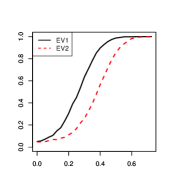
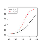
Figure 4: Local power curves $LP^{\tt MEV_{1}}(x|\bm{\psi}^{(2)},s)$ (EV1) and $LP^{\tt MEV_{2}}(x|\bm{\psi}^{(2)},s)$ (EV2) with $s=s^{(2,7)}$ (left panel), $s=s^{(2,31)}$ (middle panel) and $s=s^{(3,7)}$ (right panel), with the realization of $(s^{(3,7)}_{t}\colon 1\leq t\leq 7)=(-0.24,0.42,-1.69,0.37,0.07,1.12,-0.05)$.

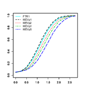
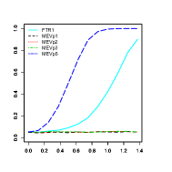
Figure 5: Local power curves $LP^{\tt FTR_{1}}(x|\bm{\psi}^{(i)},s^{(1,7)})$ and $LP^{\tt MEV_{1}}(x|\bm{\psi}^{(i)},s^{(1,7)})$ for values $p=1,2,3$ and $p=5$ and $i=1$ (left panel), $i=2$ (middle panel) and $i=3$ (right panel).

9 Summary

We have proposed several tests for detecting periodicity in functional time series which fall into two broad categories which we refer to as multivariate and fully functional approaches. Our tests are motivated by the Gaussian likelihood ratio approach, and, in general, have the expected power advantage for multivariate time series for which other tests exist. Allowing general weak dependence of errors is also new even for multivariate data. For functional data, all tests are new. In what follows we summarize the main conclusions of our work.

• Generally, the functional approach is a more adequate and safer option. The multivariate approach can be more powerful, but it is sensitive to the choice of the subspace on which the data are projected.

• If the signal is close to sinusoidal, then the simple single frequency test is more powerful, otherwise the opposite is true. The effect becomes stronger with length of the period. This empirical finding is theoretically confirmed in Appendix E of the supplement.

• For the multivariate tests we have seen that the eigenvalue statistics can have a considerable power advantage over the traditionally used trace based statistics. Theoretically, we have shown that $T^{\tt MEV_{1}}$ and $T^{\tt MEV_{2}}$ can be justified by a LR procedure when the periodic signal is proportional to a single function $w(u)$. There exists an easy algorithm to compute critical values.

If no prior knowledge on the periodic component is available, we recommend to use the ANOVA based approach or to base the decision on more than one test. Simultaneous acceptance or simultaneous rejection by several tests will lend confidence in the conclusion.

Supplemental material

Appendix A Discussion of Assumption 2.2

In this section, we explain how the test procedure should be adapted when $d$ is even. If $d=2$, then we can look at the lag-1 differenced series $\Delta Y_{t}=Y_{t}-Y_{t-1}$ and the problem boils down to testing for a zero mean of $(\Delta Y_{t})$. So assume that $d\geq 4$. The tests $T^{{\tt MTR_{1}}}$ and $T^{{\tt FTR_{1}}}$ remain unchanged. The test statistics tests $T^{{\tt MTR_{2}}}$ and $T^{{\tt FTR_{2}}}$ have to be defined in a slightly different way. We now set $r=(d-2)/2$ and replace $\bm{A}(\vartheta_{1},\ldots,\vartheta_{q})$ by

(A.1) $$\bm{B}(\vartheta_{1},\ldots,\vartheta_{r})=\left[\bm{R}(\vartheta_{1}),\ldots,\bm{R}(\vartheta_{r}),\bm{C}(\vartheta_{1}),\ldots,\bm{C}(\vartheta_{r}),\bm{R}(\theta_{N/2})\right]^{\prime}.$$

The corresponding tests in Theorem 3.1 have to be changed to

$$T^{{\tt MEV}_{2}} :=\big{\|}\bm{B}(\vartheta_{1},\ldots,\vartheta_{r})\bm{\Sigma}^{-1}\bm{B}^{\prime}(\vartheta_{1},\ldots,\vartheta_{r})\big{\|}>q_{1-\alpha}[\|\mathbf{W}_{p}(d-1)\|/2],$$

$$T^{{\tt MTR_{2}}} :=\big{\|}\bm{B}(\vartheta_{1},\ldots,\vartheta_{r})\bm{\Sigma}^{-1}\bm{B}^{\prime}(\vartheta_{1},\ldots,\vartheta_{r})\big{\|}_{\mathrm{tr}}>q_{1-\alpha}[\chi^{2}_{p(d-1)}/2],$$

respectively. The fully functional test (3.2) becomes

$$T^{{\tt FTR_{2}}}:=\sum_{k=1}^{r}\big{(}\|R(\vartheta_{k})\|^{2}+\|C(\vartheta_{k})\|^{2}\big{)}+\|R(\theta_{N/2})\|^{2}>q_{1-\alpha}\left[\sum_{k=1}^{r}\Xi_{k}+\Theta\right],$$

where $\Xi_{k}\stackrel{{\scriptstyle\mathrm{i.i.d.}}}{{\sim}}\mathrm{HExp}(\lambda_{1},\lambda_{2},\ldots)$ and $\Theta\sim\frac{1}{2}\sum_{\ell\geq 1}\lambda_{\ell}\chi^{2}(\ell)$ with i.i.d. $\chi^{2}$ variables $\chi^{2}(\ell)$. The $\lambda_{\ell}$ are the eigenvalues of $\mathrm{Var}(Y_{1})$ and $\Theta$ is independent of $\Xi_{1},\ldots,\Xi_{r}$. Accordingly, the analogue type changes are required in the setting of Section 4.

Appendix B Details of the derivation of the tests of Section 3

Proof of Theorem 3.1.

We only derive the LR test $T^{{\tt MEV_{2}}}$. Derivation of $T^{{\tt MEV_{1}}}$ is similar and $T^{{\tt MTR_{2}}}$ can be deduced from Proposition 3.1.

Set $\bm{A}=\bm{A}(\vartheta_{1},\ldots,\vartheta_{q})$ and $\bm{\gamma}=(\alpha_{1},\ldots,\alpha_{q},\beta_{1},\ldots,\beta_{q})^{\prime}$ and let $\bm{e}_{1}$ be the eigenvector associated to the largest eigenvalue of $\bm{\Sigma}^{-1/2}\bm{A}^{\prime}\bm{A}\bm{\Sigma}^{-1/2}$. The proof will reveal that the MLEs of $\bm{w}$ and $\bm{\gamma}$ are given as $\widehat{\bm{w}}=\bm{\Sigma}^{1/2}\bm{e}_{1}$ and $\widehat{\bm{\gamma}}=\frac{2}{\sqrt{N}}\bm{A}\bm{\Sigma}^{-1/2}\bm{e}_{1}$, respectively. We notice that $\widehat{\bm{w}}$ and $\widehat{\bm{\gamma}}$ are not unique. For any $x>0$, the pair $(\widehat{\bm{w}},\widehat{\bm{\gamma}})$ maybe replaced by $(x\widehat{\bm{w}},\widehat{\bm{\gamma}}/x)$. If the largest eigenvalue of $\bm{\Sigma}^{-1/2}\bm{A}^{\prime}\bm{A}\bm{\Sigma}^{-1/2}$ has multiplicity one, then uniqueness can be obtained imposing $\|\widehat{\bm{w}}\|=1$.

Define $\bm{c}_{i}=\big{(}\cos(t\vartheta_{i})\colon 1\leq t\leq N\big{)}^{\prime}$ and $\bm{s}_{i}=\big{(}\sin(t\vartheta_{i})\colon 1\leq t\leq N\big{)}^{\prime}$. Moreover we set $\bm{w}^{\mathrm{sc}}=\mathbf{\Sigma}^{-1/2}\bm{w}$ and $\bm{Y}_{t}^{\mathrm{sc}}=\mathbf{\Sigma}^{-1/2}\bm{Y}_{t}$. First we observe that under $\mathcal{H}_{0}$ as well as under $\mathcal{H}_{A}$ the MLE for $\bm{\mu}=\overline{\bm{Y}}$. Using representation (2.5) of the underlying model, mutual orthogonality of the vectors $\bm{c}_{1},\ldots,\bm{c}_{q},\bm{s}_{1},\ldots,\bm{s}_{q}$ and $\|\bm{c}_{i}\|=\|\bm{s}_{i}\|=N/2$, we obtain with simple algebra that the log-likelihood ratio is given by  $\max_{\bm{w}^{\mathrm{sc}},\bm{\gamma}}\ell_{N}(\bm{w}^{\mathrm{sc}},\bm{\gamma})$, where

$$\ell_{N}(\bm{w}^{\mathrm{sc}},\bm{\gamma})=\big{(}\bm{w}^{\mathrm{sc}}\big{)}^{\prime}\bm{\Sigma}^{-1/2}\bm{A}^{\prime}\bm{\gamma}-\frac{\sqrt{N}}{4}\|\bm{w}^{\mathrm{sc}}\|^{2}\|\bm{\gamma}\|^{2}.$$

Since for any $x>0$ we have $\ell_{N}(\bm{w}^{\mathrm{sc}},\bm{\gamma})=\ell_{N}(x\bm{w}^{\mathrm{sc}},\bm{\gamma}/x)$, we can assume that $\|\bm{w}^{\mathrm{sc}}\|=1$. Under this constraint we maximize

$$\ell_{N}(\bm{w}^{\mathrm{sc}},\bm{\gamma})=\big{(}\bm{w}^{\mathrm{sc}}\big{)}^{\prime}\bm{\Sigma}^{-1/2}\bm{A}^{\prime}\bm{\gamma}-\frac{\sqrt{N}}{4}\|\bm{\gamma}\|^{2}.$$

For given $\bm{w}^{\mathrm{sc}}$ we obtain the maximizer $\widehat{\bm{\gamma}}=\frac{2}{\sqrt{N}}\bm{A}\bm{\Sigma}^{-1/2}\bm{w}^{\mathrm{sc}}$ and

$$\max_{\bm{w}^{\mathrm{sc}}\colon\|\bm{w}^{\mathrm{sc}}\|=1}\ell(\widehat{\bm{\gamma}},\bm{w}^{\mathrm{sc}}) =\frac{1}{\sqrt{N}}\max_{\bm{w}^{\mathrm{sc}}\colon\|\bm{w}^{\mathrm{sc}}\|=1}\big{(}\bm{w}^{\mathrm{sc}}\big{)}^{\prime}\bm{\Sigma}^{-1/2}\bm{A}^{\prime}\bm{A}\bm{\Sigma}^{-1/2}\bm{w}^{\mathrm{sc}}$$

$$=\frac{1}{\sqrt{N}}\|\bm{\Sigma}^{-1/2}\bm{A}^{\prime}\bm{A}\bm{\Sigma}^{-1/2}\|=\frac{1}{\sqrt{N}}\|\bm{A}\bm{\Sigma}^{-1}\bm{A}^{\prime}\|.$$

Moreover, the maximizing $\bm{w}^{\mathrm{sc}}=\bm{e}_{1}$. ∎

Lemma B.1.

Under Assumption 2.1 and $\mathcal{H}_{0}$ we have that

$$\big{(}R(\theta_{1}),\ldots,R(\theta_{m}),C(\theta_{1})\cdots,C(\theta_{m})\big{)}$$

are i.i.d. elements in $H$. We have $R(\theta_{1})\sim\mathcal{N}_{H}(0,\frac{1}{2}\Gamma)$. The analogous result holds if the functions $R(\theta_{i})$ and $C(\theta_{i})$ are replaced by their projections $\mathbf{R}(\theta_{i})$ and $\mathbf{C}(\theta_{i})$. In this case we have $\mathbf{R}(\theta_{i})\sim\mathcal{N}_{p}(0,\frac{1}{2}\bm{\Sigma})$.

Proof.

Clearly, the vectors are jointly Gaussian. Recall that $\theta_{j}\in\Theta_{N}$ are the fundamental frequencies. Set $\bm{c}(\theta)=\big{(}\cos(t\theta)\colon 1\leq t\leq N\big{)}^{\prime}$ and $\bm{s}(\theta)=\big{(}\sin(t\theta)\colon 1\leq t\leq N\big{)}^{\prime}$, then the result is a simple consequence of the fact that the vectors $(\bm{c}(\theta)\colon\theta\in\Theta_{N})$ and $(\bm{s}(\theta)\colon\theta\in\Theta_{N})$ are mutually orthogonal and with norm $N/2$. ∎

Lemma B.2.

Under Assumption 2.1 and $\mathcal{H}_{0}$ we have that

$$\|A(\vartheta_{1},\ldots,\vartheta_{q})A^{\prime}(\vartheta_{1},\ldots,\vartheta_{q})\|_{\mathrm{tr}}\sim\sum_{i=1}^{q}\Xi_{i},$$

where $\Xi_{1},\ldots,\Xi_{q}$ are i.i.d. random variables distributed as $\mathrm{HExp}(\lambda_{1},\lambda_{2},\ldots)$ and $(\lambda_{k})$ are the eigenvalues of $\Gamma$ .

Proof.

Let $(v_{k})$ be the eigenvectors of $\Gamma$. By Parseval’s identity we have $\|R(\theta)\|^{2}=\sum_{k\geq 1}\langle R(\theta),v_{k}\rangle^{2}$ and $\|C(\theta)\|^{2}=\sum_{k\geq 1}\langle C(\theta),v_{k}\rangle^{2}$. By Lemma B.1 it follows that $\langle R(\theta),v_{k}\rangle,\langle C(\theta),v_{k}\rangle$ are independent Gaussian with zero mean and variance $\lambda_{k}/2$. The result follows easily from $\|A(\vartheta_{1},\ldots,\vartheta_{q})A^{\prime}(\vartheta_{1},\ldots,\vartheta_{q})\|_{\mathrm{tr}}=\sum_{k=1}^{q}\big{(}\|R(\vartheta_{k})\|^{2}+\|C(\vartheta_{k})\|^{2}\big{)}$. ∎

Proof of Proposition 3.1.

We verify the identity in the functional case.

$$\sum_{k=1}^{q}\left(\left\|R(\vartheta_{k})\right\|^{2}+\left\|C(\vartheta_{k})\right\|^{2}\right)$$

$$\quad=\sum_{k=1}^{q}\left(\left\|\frac{n}{\sqrt{N}}\sum_{t=1}^{d}(\overline{Y}_{t}-\overline{Y})\cos(\vartheta_{k}t)\right\|^{2}+\left\|\frac{n}{\sqrt{N}}\sum_{t=1}^{d}(\overline{Y}_{t}-\overline{Y})\sin(\vartheta_{k}t)\right\|^{2}\right)$$

$$\quad=\frac{n}{d}\sum_{t=1}^{d}\sum_{s=1}^{d}\langle\overline{Y}_{t}-\overline{Y},\overline{Y}_{s}-\overline{Y}\rangle\sum_{k=1}^{q}\left(\cos(\vartheta_{k}t)\cos(\vartheta_{k}s)+\sin(\vartheta_{k}t)\sin(\vartheta_{k}s)\right)$$

$$\quad=\frac{n}{d}\sum_{t=1}^{d}\sum_{s=1}^{d}\langle\overline{Y}_{t}-\overline{Y},\overline{Y}_{s}-\overline{Y}\rangle\left(qI\{t=s\}-1/2I\{t\neq s\}\right)$$

$$\quad=\frac{n}{2}\sum_{t=1}^{d}\|\overline{Y}_{t}-\overline{Y}\|^{2}-\frac{1}{2}\sum_{t=1}^{d}\sum_{s=1}^{d}\langle\overline{Y}_{t}-\overline{Y},\overline{Y}_{s}-\overline{Y}\rangle$$

$$\quad=\frac{1}{2}\sum_{t=1}^{d}n\lVert\overline{Y}_{t}-\overline{Y}\rVert^{2}.$$

∎

Appendix C Proofs of the results of Sections 4 and 5

Proof of Proposition 4.1.

According to Theorem 4.1 we have that the vector of functions $(D_{N}^{Z}(\vartheta_{1}),\ldots,D_{N}^{Z}(\vartheta_{q}))$ will converge weakly to a $q$–vector $\big{(}\mathcal{N}_{1},\ldots,\mathcal{N}_{q}\big{)}\in H^{k}$ where $\mathcal{N}_{k}\stackrel{{\scriptstyle\text{ind}}}{{\sim}}\mathcal{CN}_{H}(0,\mathcal{F}_{\vartheta_{k}})$. Hence, $\|R_{N}^{Z}(\vartheta_{k})\|^{2}+\|C_{N}^{Z}(\vartheta_{k})\|^{2}=\|D_{N}^{Z}(\vartheta_{k})\|^{2}\stackrel{{\scriptstyle d}}{{\to}}\|\mathcal{N}_{k}\|^{2}$. For any $\theta\in[-\pi,\pi]$ the operator $\mathcal{F}_{\theta}$ is trace class, symmetric and non-negative definite. So it possesses the same properties as a covariance operator. In particular we have a spectral decomposition of the form $\mathcal{F}_{\theta}=\sum_{m\geq 1}\lambda_{m}(\theta)\varphi_{m}(\theta)\otimes\varphi_{m}(\theta)$, where $\lambda_{m}(\theta)\geq 0$ are the eigenvalues (in descending order) and $\varphi_{m}(\theta)$ are the corresponding (possibly complex valued) eigenfunctions of $\mathcal{F}_{\theta}$. By Parceval’s identity

(C.1) $$\|\mathcal{N}_{k}\|^{2}=\sum_{m\geq 1}\langle\mathcal{N}_{k},\varphi_{m}(\vartheta_{k})\rangle\overline{\langle\mathcal{N}_{k},\varphi_{m}(\vartheta_{k})\rangle}.$$

The $(\varphi_{m}(\vartheta_{k})\colon m\geq 1)$ are, in fact, the principal components of $\mathcal{N}_{k}$. By their orthogonality, the normal scores $(\langle\mathcal{N}_{k},\varphi_{m}(\vartheta_{k})\rangle\colon m\geq 1)$ are independent $\mathcal{CN}\big{(}0,\lambda_{m}(\vartheta_{k})\big{)}$. Hence, $(\mathrm{Re}(\langle\mathcal{N}_{k},\varphi_{m}(\vartheta_{k})\rangle)$, $\mathrm{Im}(\langle\mathcal{N}_{k},\varphi_{m}(\vartheta_{k})\rangle))\sim(N_{1},N_{2})$ where $N_{1}$ and $N_{2}$ are i.i.d. $N(0,\lambda_{m}(\vartheta_{k})/2)$. It implies that that $m$-th term of the sum in (C.1) is distributed as $\lambda_{m}(\vartheta_{k})\times\mathrm{Exp}(1)$.

∎

Proof of Proposition 5.1.

From the definition of $A(\vartheta_{1},\ldots,\vartheta_{q})$ and (5.1) we deduce

$$\|A(\vartheta_{1},\ldots,\vartheta_{q})A^{\prime}(\vartheta_{1},\ldots,\vartheta_{q})\|_{\mathrm{tr}}=\sum_{j=1}^{q}\|D^{Y}_{N}(\vartheta_{j})\|^{2}$$

$$\quad=\sum_{j=1}^{q}\left[\|D^{Z}_{N}(\vartheta_{j})\|^{2}+n\|D^{w}_{d}(\vartheta_{j})\|^{2}+2\sqrt{n}\,\mathrm{Re}\big{(}\langle D^{w}_{d}(\vartheta_{j}),D^{Z}_{N}(\vartheta_{j})\rangle\big{)}\right].$$

When the noise satisfies the assumptions in Theorem 4.1, then it follows that each term $\|D^{Z}_{N}(\vartheta_{j})\|^{2}=O_{P}(1)$. ∎

Proof of Proposition 5.2.

This goes along the lines of the proof of Proposition 5.1. ∎

Appendix D Estimation of covariance and spectral density

To implement the tests developed in Section 3, we have to estimate $\mathbf{\Sigma}$ and $\Gamma$. The tests of Section 4 require the estimation of a spectral density. In the following we will outline the estimation problem in the fully functional setting. The key point is to derive estimators which are consistent under $\mathcal{H}_{0}$ and $\mathcal{H}_{A}$. Failing to be consistent under $\mathcal{H}_{A}$, may still lead to consistent tests, but can have a strong negative impact on the power of the tests.

We recall that $C_{h}=\mathrm{Cov}(Y_{t+h},Y_{t})$ is the lag-$h$ autocovariance operator of the time series $(X_{t})$ and hence $C_{0}=\Gamma$. We stress that under the general model (M.3), the process $(X_{t})$ is covariance stationary. Once we have estimators $\widehat{w}_{t}=\widehat{w}_{t+d}$ (we will require $\sum_{t=1}^{d}\widehat{w}_{t}=0$) it is natural to set

(D.1) $$\widehat{C}_{h}=\frac{1}{N}\sum_{t=1}^{N-h}(Y_{t+h}-\widehat{w}_{t+h}-\overline{Y})\otimes(Y_{t}-\widehat{w}_{t}-\overline{Y}).$$

The following lemma translates the consistency rate for $\widehat{w}_{t}$ to a rate for $\widehat{C}_{h}$. We let $\|\cdot\|_{\mathcal{S}}$ be the Hilbert-Schmidt norm on the set of compact operators on $H$ and use $c_{0},c_{1},c_{2}$ for constants that do not depend on $N$ and $h$.

Lemma D.1.

Consider model (M.3), Assumption 2.2 and assume that $(Z_{t})$ is $L^{4}$-$m$–approximable. Assume further that $NE\|\widehat{w}_{t}-w_{t}\|^{2}$ is bounded by some constant $b_{0}$ for all $t,N\geq 1$. Then

$$E\|\widehat{C}_{h}-C_{h}\|_{\mathcal{S}}\leq c_{0}\sqrt{\frac{|h|\vee 1}{N}}.$$

The most simple estimator is $\widehat{w}_{t}=\overline{Y}_{t}-\overline{Y}$. Under $L^{2}$-$m$–approximability this estimator satisfies the consistency assumption of the lemma.

Proof.

Set $\nu_{2}(X)=\big{(}E\|X\|^{2}\big{)}^{1/2}$ and assume without loss of generality that $h\geq 0$. Let us first remark that $\overline{Y}=\mu+\overline{Z}$ and that basic properties for $L^{2}$-$m$–approximable sequences lead to

(D.2) $$NE\|\overline{Z}\|^{2}\leq 2\nu_{2}(Z_{0})\sum_{k\geq 0}\nu_{2}(Z_{0}-Z_{0}^{(k)})=:c_{1}.$$

Then we decompose $(Y_{t+h}-\widehat{w}_{t+h}-\overline{Y})\otimes(Y_{t}-\widehat{w}_{t}-\overline{Y})-C_{h}$ into

$$[Z_{t+h}\otimes Z_{t}-C_{h}]+(w_{t+h}-\widehat{w}_{t+h})\otimes(w_{t}-\widehat{w}_{t})+\overline{Z}\otimes\overline{Z}$$

$$\qquad-\big{[}\overline{Z}\otimes(w_{t}-\widehat{w}_{t})+(w_{t+h}-\widehat{w}_{t+h})\otimes\overline{Z}\big{]}$$

$$\qquad-\big{[}\overline{Z}\otimes Z_{t}+Z_{t+h}\otimes\overline{Z}\big{]}$$

$$\qquad+\big{[}(w_{t+h}-\widehat{w}_{t+h})\otimes Z_{t}+Z_{t+h}\otimes(w_{t}-\widehat{w}_{t})\big{]}=:\sum_{j=1}^{9}A_{t}^{(j)}.$$

For each $j\in\{1,\ldots,9\}$ we need a bound for $\kappa_{j}:=\frac{1}{N}E\|\sum_{t=1}^{N-h}A_{t}^{(j)}\|_{\mathcal{S}}$. Let us also introduce $\tilde{\kappa}_{j}:=\frac{1}{N}E\|\sum_{t=1}^{N}A_{t}^{(j)}\|_{\mathcal{S}}$ and note that $\kappa_{j}\leq\tilde{\kappa}_{j}+\frac{h}{N}\max E\|A_{t}^{(j)}\|_{\mathcal{S}}$.

By Lemma 4 in [2015] we have that $\kappa_{1}\leq c_{2}\sqrt{\frac{h\vee 1}{N}}$. Then since

$$\sum_{t=1}^{N}A_{t}^{(2)}=n\sum_{k=1}^{d}(w_{k+h}-\widehat{w}_{k+h})\otimes(w_{k}-\widehat{w}_{k}),$$

we have that $\tilde{\kappa}_{2}\leq\frac{b_{0}}{N}$ and thus $\kappa_{2}\leq\frac{b_{0}}{N}(1+\frac{h}{N})$. By (D.2) we have $\kappa_{3}=E\|\overline{Z}\|^{2}\leq\frac{c_{1}}{N}$. Next, by the assumptions on $w_{t}$ and $\widehat{w}_{t}$ we have $\tilde{\kappa}_{4}=\ \tilde{\kappa}_{5}=0$ and hence $\kappa_{4},\kappa_{5}\leq\sqrt{\frac{c_{1}}{N}\frac{b_{0}}{N}}\big{(}1+\frac{h}{N}\big{)}.$ Again by (D.2) it follows that $\kappa_{6},\kappa_{7}\leq\frac{c_{1}}{N}$. Finally, it can be shown along the same lines that $\kappa_{8},\kappa_{9}\leq\sqrt{\frac{dc_{1}}{N}\frac{b_{0}}{N}}$. The proof follows by collecting all terms. ∎

A simple implication of this lemma is that whenever we have $L^{2}$ consistent estimators for $w_{t}$, then $\widehat{\Gamma}=\widehat{C}_{0}$ is a consistent estimator of $\Gamma$.

Turning to the estimation of the spectral density, we propose a lag window estimator of the form

(D.3) $$\mathcal{\widehat{F}}_{\theta}=\sum_{|h|\leq b_{N}}\gamma\left(\frac{h}{b_{N}}\right)\widehat{C}_{h}e^{-\mathrm{i}h\theta},\quad 0<b_{N}<N,$$

where the function $\gamma$ is continuous in zero and such that $\gamma(0)=1$, $\lvert\gamma(x)\rvert\leq 1,\;\forall x$ and $\gamma(x)=0$ for $\lvert x\rvert>1$. The bandwidth satisfies $b_{N}\to\infty$ and ${b_{N}}/{N}\to 0$, with more specific rate stated in the next proposition.

Proposition D.1.

Consider the setup of Lemma D.1 and suppose that $b_{N}\to\infty$, such that $b_{N}=o\big{(}N^{1/3}\big{)}$. Then  $\sup_{\theta\in[-\pi,\pi]}\|\mathcal{F}_{\theta}-\mathcal{\widehat{F}}_{\theta}\|_{\mathcal{S}}\to 0$ in probability.

Proof.

We will adapt the proof of Proposition 4 of [2015] to our setting. By definition of the estimator and by using the triangular inequality, we have

$$\lVert\mathcal{F}_{\theta}-\widehat{\mathcal{F}}_{\theta}\rVert_{\mathcal{S}} =\left\|\sum_{h\in\mathbb{Z}}C_{h}e^{-ih\theta}-\sum_{\lvert h\rvert\leq b_{N}}\gamma\left(\frac{h}{b_{N}}\right)\widehat{C}_{h}e^{-i\theta h}\right\|_{\mathcal{S}}$$

$$\leq\sum_{\lvert h\rvert\leq b_{N}}\left(\|C_{h}-\widehat{C}_{h}\|_{\mathcal{S}}+|1-\gamma(h/b_{N})|\|C_{h}\|_{\mathcal{S}}\right)+\sum_{|h|>b_{N}}\|C_{h}\|_{\mathcal{S}}.$$

Taking expectations, we obtain by Lemma D.1

$$E\lVert\mathcal{F}_{\theta}-\widehat{\mathcal{F}}_{\theta}\rVert_{\mathcal{S}}\leq 2c_{0}\sqrt{\frac{b_{N}^{3}}{N}}+\sum_{\lvert h\rvert\leq b_{N}}|1-\gamma(h/b_{N})|\|C_{h}\|_{\mathcal{S}}+\sum_{|h|>b_{N}}\|C_{h}\|_{\mathcal{S}}.$$

By our assumptions, all three terms on the right hand side tend to zero. For the first, this is immediate from our assumption on $b_{N}$. For the third we use (4.2) and for the second dominated convergence. ∎

It is an immediate consequence of Proposition D.1 and Corollary 1.6 on p. 99 of [1990] that

$$\sup_{\theta\in[-\pi,\pi]}\sup_{m\geq 1}|\lambda_{m}(\theta)-\hat{\lambda}_{m}(\theta)|=o_{P}(1),$$

justifying the approximation of the model eigenvalues by the estimated eigenvalues.

Appendix E Local consistency

In this section we focus for brevity only on the functional test statistics $T^{\tt FTR_{1}}$ and $T^{\tt FAV}$ (or equivalently $T^{\tt FTR_{2}}$). The multivariate tests require additional tuning (choice of the basis). For a fixed basis the discussion below can be done analogously.

We consider consistency of the test, when the alternative shrinks to the null with growing sample size. An important finding of this section is that if the period $d$ is relatively large, and if we expect a smooth change for the periodic trend, the test based on $T^{\tt FTR_{1}}$ is preferable to the ANOVA approach. In contrast, if the periodic signal is more erratic, the ANOVA approach has better local power features. This confirms simulation results in Section 8.

More specifically we consider here local alternatives $(w_{t}(u)\colon 1\leq t\leq d)$, with mean square sum of the signal $\text{MSS}_{\text{sig}}=\frac{1}{d}\sum_{k=1}^{d}\|w_{k}\|^{2}=\varrho^{2}\to 0$. We analyze three scenarios for $\mathcal{H}_{A}$. In each we define $w_{t}=\omega_{t}-\bar{\omega}$ with $\bar{\omega}=\frac{1}{d}\sum_{k=1}^{d}\omega_{k}$. Then we consider for some $\varrho^{2}>0$ the following:

1. $\omega_{t}$ are orthogonal functions with $\|\omega_{t}\|^{2}=\frac{d}{d-1}\varrho^{2}$ ;

2. $\omega_{t}=\omega_{0}\big{[}\cos(2\pi t/d)+\sin(2\pi t/d)\big{]}$ with $\|\omega_{0}\|^{2}=\varrho^{2}$ ;

3. $\omega_{t}=\frac{1}{\sqrt{d}}\big{(}\sum_{k=1}^{t}v_{k}-\frac{t}{d}\sum_{k=1}^{d}v_{k}\big{)}$ for orthogonal functions $v_{k}\in H$ with scaling $\lVert v_{k}\rVert^{2}=\frac{12d^{2}}{d^{2}-1}\varrho^{2}$.

Straightforward computations show that indeed for (A)–(C) we have $\text{MSS}_{\text{sig}}=\varrho^{2}.$

In setting (A) the periodic pattern is extremely irregular and intuitively it should be very unfavorable for the test based on $T^{\tt FTR_{1}}$ since there is no sinusoidal trend involved. In contrast, scenario (B) is tailor-made for this test. Finally, scenario (C) is supposed to provide a realistic alternative. It is based on the assumption that the periodic trend $(w_{t})$ changes smoothly. Orthogonality of the $v_{k}$ is only imposed to make $\text{MSS}_{\text{sig}}$ computable.

Next we define the power functions

$$\kappa_{1}(\alpha)=P\big{(}T^{\tt FTR_{1}}>q_{1-\alpha}^{(1)}\big{)}\quad\text{and}\quad\kappa_{2}(\alpha)=P\big{(}T^{\tt FAV}>q_{1-\alpha}^{(2)}\big{)},$$

where $q_{1-\alpha}^{(1)}$ and $q_{1-\alpha}^{(2)}$ are the $(1-\alpha)$–quantiles of the respective null-distributions.

Proposition E.1.

Let $\alpha\in(0,1)$ and assume that $\varrho^{2}=\varrho_{n}^{2}\to 0$ with $n\to\infty$. We impose Assumption 2.1. Then the following claims hold.

1. When $n\varrho_{n}^{2}\to\infty$, both power functions $\kappa_{1}(\alpha)$ and $\kappa_{2}(\alpha)$ tend to one under all three alternatives.

2. When $n\varrho_{n}^{2}\to 0$ both power functions $\kappa_{1}(\alpha)$ and $\kappa_{2}(\alpha)$ tend to $\alpha$ under all three alternatives.

3. Suppose $d=d_{n}\to\infty$ and $n\varrho_{n}^{2}\to 0$. Then $\kappa_{2}(\alpha)\to\begin{cases}1&\text{if $\sqrt{d_{n}}n\varrho_{n}^{2}\to\infty$;}\\ \alpha&\text{if $\sqrt{d_{n}}n\varrho_{n}^{2}\to 0$}.\end{cases}$

4. Suppose $d=d_{n}\to\infty$ and $n\varrho_{n}^{2}\to 0$. Under alternative (A) $\kappa_{1}(\alpha)\to\alpha$ while under alternatives (B) and (C) we have that $\kappa_{1}(\alpha)\to\begin{cases}1&\text{if $d_{n}n\varrho_{n}^{2}\to\infty$;}\\ \alpha&\text{if $d_{n}n\varrho_{n}^{2}\to 0$.}\end{cases}$

This proposition shows that whether one of the tests is asymptotically consistent or not, is determined by $n\varrho_{n}^{2}\to\infty$ and $n\varrho_{n}^{2}\to 0$, respectively. The interesting case is when $n\varrho_{n}^{2}\to 0$ and at the same time $d=d_{n}\to\infty$. Here under setup (A) the statistic $T^{\tt FAV}$ is preferable since it can still provide a consistent test. On the other hand, statement 4 of the proposition shows superiority of $T^{\tt FTR_{1}}$ under a local alternative related to settings (B) and (C). In these cases $T^{\tt FTR_{1}}$ allows additional shrinking the alternative by a factor $1/\sqrt{d_{n}}$ compared $T^{\tt FAV}$ in order to remain consistent.

Proof of Proposition E.1.

Denote by $\|M^{Y}_{N}(\vartheta_{1})\|_{\mathrm{tr}},\;\|M^{Z}_{N}(\vartheta_{1})\|_{\mathrm{tr}}$ and $\|M^{w}_{d}(\vartheta_{1})\|_{\mathrm{tr}}$ the trace statistics based on the time series $Y_{t}$, $Z_{t}$ $(t=1,\ldots,N)$ and $w_{t}$ $(t=1,\ldots,d)$. From (5.1) one easily deduce that

$$\|M^{Y}_{N}(\vartheta_{1})\|_{\mathrm{tr}}=\|M^{Z}_{N}(\vartheta_{1})\|_{\mathrm{tr}}+n\|M^{w}_{d}(\vartheta_{1})\|_{\mathrm{tr}}+O_{P}\Big{(}\big{(}n\|M^{w}_{d}(\vartheta_{1})\|_{\mathrm{tr}}\big{)}^{1/2}\Big{)}.$$

The trace statistics of the periodic signal for alternatives (A), (B) and (C) are, respectively, $\frac{d}{d-1}n\varrho_{n}^{2}$, $dn\varrho^{2}_{n}$ and $\frac{3dn\varrho^{2}_{n}}{(d^{2}-1)\sin^{2}(\pi/d)}$. Consider, for example, alternative (A). Then

$$P(\|M^{Y}_{N}(\vartheta_{1})\|_{\mathrm{tr}}>q_{1-\alpha}^{(1)}) =P\left(\|M^{Z}_{N}(\vartheta_{1})\|_{\mathrm{tr}}>q_{1-\alpha}^{(1)}-\frac{d}{d-1}n\varrho^{2}_{n}+O_{P}\bigg{(}\sqrt{\frac{d}{d-1}n\varrho^{2}_{n}}\bigg{)}\right).$$

To verify claims 1,2 and 4 related to the trace based statistic, it suffices to observe that this probability tends to $\alpha$ if $n\varrho^{2}_{n}\to 0$ and to 1 if $n\varrho^{2}_{n}\to\infty$. The statements under alternatives (B) and (C^′) are proven analogously.

Concerning statistic $T^{\tt FAV}$ we first note that by the assumption $\mathrm{MSS}_{\mathrm{sig}}=\varrho_{n}^{2}$ it readily follows that

$$\frac{n}{d}\sum_{k=1}^{d}\langle w_{k},\overline{Z}_{k}-\overline{Z}\rangle=\frac{n}{d}\sum_{k=1}^{d}\langle w_{k},\overline{Z}_{k}\rangle=O_{P}\big{(}\sqrt{n\varrho_{n}^{2}/d}\big{)}.$$

With this one can easily prove that

$$P(T^{\tt FAV}>q_{1-\alpha}^{2})=P\Big{(}T^{\tt FAV}(Z)>q_{1-\alpha}^{2}-n\varrho_{n}^{2}+O_{P}\big{(}\sqrt{n\varrho_{n}^{2}/d}\big{)}\Big{)}.$$

Here $T^{\tt FAV}(Z)$ is the ANOVA statistic computed from the noise. Claims 1 and 2 are immediate.

We show claim 3. Let us impose for simplicity that Assumption 2.2 holds. Then, since by Gaussianity the distribution of $T^{\tt FAV}(Z)$ is independent of $n$, we get by Corollary 4.1 that

$$P(T^{\tt FAV}(Y)>q_{1-\alpha}^{2})=P\Big{(}\frac{2}{d}\sum_{k=1}^{q}\Xi_{k}>q_{1-\alpha}^{\text{FAV}}-n\varrho_{n}^{2}+O_{P}(\sqrt{n\varrho_{n}^{2}/d})\Big{)}$$

$$\,=P\left(\frac{1}{\sqrt{q}}\sum_{k=1}^{q}(\Xi_{k}-E\Xi_{1})>q_{1-\alpha}\left[\frac{1}{\sqrt{q}}\sum_{k=1}^{q}(\Xi_{k}-E\Xi_{1})\right]-\frac{dn\varrho_{n}^{2}}{2\sqrt{q}}+O_{P}(\sqrt{n\varrho_{n}^{2}d/q})\right).$$

By the central limit theorem $\frac{1}{\sqrt{q}}\sum_{k=1}^{q}(\Xi_{k}-E\Xi_{1})\stackrel{{\scriptstyle d}}{{\to}}N(0,\mathrm{Var}(\Xi_{1}))$ and hence the quantiles $q_{1-\alpha}\left[\frac{1}{\sqrt{q}}\sum_{k=1}^{q}(\Xi_{k}-E\Xi_{1})\right]$ will converge to the corresponding normal quantile for $d\to\infty$. From this it is easy to conclude. ∎

References

- Aue et al. (2015) Aue, A., Dubart-Norinho, D. and Hörmann, S. (?). On the prediction of stationary functional time series. Journal of the American Statistical Association, 110, 378–392.
- 1991 Brockwell, P. J. and Davis, R. A. (?). Time Series: Theory and Methods. Springer, New York.
- 2015 Cerovecki, C. and Hörmann, S. (?). A note on the CLT for the discrete fourier transforms of functional time series. Working paper. Université libre de Bruxelles.
- 2014 Chiani, M. (?). Distribution of the largest eigenvalue for real Wishart and Gaussian random matrices and a simple approximation for the Tracy–Widom distribution. Journal of Multivariate Analysis, 129, 68–81.
- 2004 Cuevas, A., Febrero, M. and Fraiman, R. (?). An ANOVA test for functional data. Computational Statistics and Data Analysis, 47, 111–122.
- 1929 Fisher, R. A. (?). Tests of significance in harmonic analysis. Proceedings of the Royal Society (A), 125, 54–59.
- 1990 Gohberg, I., Golberg, S. and Kaashoek, M. A. (?). Classes of Linear Operators. Operator Theory: Advances and Applications, volume 49. Birkhaüser.
- 2016 Gromenko, O., Kokoszka, P. and Reimherr, M. (?). Detection of change in the spatiotemporal mean function. Journal of the Royal Statistical Society (B), 00, 00–00; Forthcoming.
- 1961 Hannan, E.J. (?). Testing for a jump in the spectral function. Journal of the Royal Statistical Society. Series (B), 23, number 2, 394–404.
- 2012 Hays, S., Shen, H. and Huang, J. Z. (?). Functional dynamic factor models with application to yield curve forecasting. The Annals of Applied Statistics, 6, 870–894.
- 2013 Hörmann, S., Horváth, L. and Reeder, R. (?). A functional version of the ARCH model. Econometric Theory, 29, 267–288.
- 2015 Hörmann, S., Kidziński, L. and Hallin, M. (?). Dynamic functional principal components. Journal of the Royal Statistical Society (B), 77, 319–348.
- 2010 Hörmann, S. and Kokoszka, P. (?). Weakly dependent functional data. The Annals of Statistics, 38, 1845–1884.
- 2012 Horváth, L. and Kokoszka, P. (?). Inference for Functional Data with Applications. Springer.
- 2014 Horváth, L., Kokoszka, P. and Rice, G. (?). Testing stationarity of functional time series. Journal of Econometrics, 179, 66–82.
- 2015 Hsing, T. and Eubank, R. (?). Theoretical Foundations of Functional Data Analysis, with an Introduction to Linear Operators. Wiley.
- 1957 Jenkins, G. M. and Priestley, M. B. (?). The spectral analysis of time-series. Journal of the Royal Statistical Society. Series (B), 19, number 1, 1–12.
- 2008 Jun, M. and Stein, M. L. (?). Nonstationary covariance models for global data. The Annals of Applied Statistics, 2, 1271–1289.
- 2016 Klepsch, J., Klüppelberg, C. and Wei, T. (?). Prediction of functional ARMA processes with an application to traffic data. Technical Report. TU München.
- 1974 MacNeill, I. B. (?). Tests for periodic components in multiple time series. Biometrika, 61, 57–70.
- 1979 Mardia, K.V., Kent, J.T. and Bibby, J.M. (?). Multivariate Analysis. Academic Press, London.
- 2013a Panaretos, V. M. and Tavakoli, S. (?). Cramér–Karhunen–Loève representation and harmonic principal component analysis of functional time series. Stochastic Processes and their Applications, 123, 2779–2807.
- 2013b Panaretos, V. M. and Tavakoli, S. (?). Fourier analysis of stationary time series in function space. The Annals of Statistics, 41, 568–603.
- 2009 Ramsay, J., Hooker, G. and Graves, S. (?). Functional Data Analysis with R and MATLAB. Springer.
- 2010 Ross, S. (?). Introduction to Probability Models. Elsevier.
- 2007 Sarty, G. (?). Computing Brain Activity Maps from fMRI Time-Series Images. Cambidge.
- 1898 Schuster, A. (?). On the investigation of hidden periodicities with application to the supposed 26 day period od meteorological phenomena. Terr. Mag., 3, 13–41.
- 2007 Shao, X. and Wu, W. B. (?). Asymptotic spectral theory for nonlinear time series. The Annals of Statistics, 35, 1773–1801.
- 2004 Stadlober, E. and Pfeiler, B. (?). Explorative Analyse der Feinstaub-Konzentrationen von Oktober 2003 bis März 2004. Technical Report. TU Graz.
- 2008 Stadtlober, E., Hörmann, S. and Pfeiler, B. (?). Quality and performance of a PM10 daily forecasting model. Athmospheric Environment, 42, 1098–1109.
- 1914 Walker, G. (?). On the criteria for the reality of relationships or periodicities. Calcutta Ind. Met. Memo, 21, number 9.
- 2005 Wu, W. (?). Nonlinear System Theory: Another Look at Dependence, volume 102. The National Academy of Sciences of the United States.
- 2016 Zamani, A., Haghbin, H. and Shishebor, Z. (?). Some tests for detecting cyclic behavior in functional time series with application in climate change. Technical report. Shiraz University.
- 2016 Zhang, X. (?). White noise testing and model diagnostic checking for functional time series. Journal of Econometrics, 194, 76–95; Forthcoming.