Optimal convection cooling flows in general geometries

Abstract

We generalize a recent method for computing optimal 2D convection cooling flows in a horizontal layer to a wide range of geometries, including those relevant for technological applications. We write the problem in a conformal pair of coordinates which are the pure conduction temperature and its harmonic conjugate. We find optimal flows for cooling a cylinder in an annular domain, a hot plate embedded in a cold surface, and a channel with hot interior and cold exterior. With a constraint of fixed kinetic energy, the optimal flows are all essentially the same in the conformal coordinates. In the physical coordinates, they consist of vortices ranging in size from the length of the hot surface to a small cutoff length at the interface of the hot and cold surfaces. With the constraint of fixed enstrophy (or fixed rate of viscous dissipation), a geometry-dependent metric factor appears in the equations. The conformal coordinates are useful here because they map the problems to a rectangular domain, facilitating numerical solutions. With a small enstrophy budget, the optimal flows are dominated by vortices which have the same size as the flow domain.

1 Introduction

Heat transfer plays a fundamental role in many problems of scientific, environmental, and technological importance (Raschke (1960); Rohsenow et al. (1985); Ozisik (2000); Otero et al. (2004); Doering et al. (2006); Lienhard (2013)). Heat transfer by the natural and forced convection of fluids leads to many important fluid dynamics problems across science and engineering (Bird et al. (2007); Bejan (2013); Lienhard (2013)). For example, several studies have proposed methods for increasing heat transfer efficiency to alleviate constraints on computer processor speeds due to internal heating (Nakayama (1986); Zerby & Kuszewski (2002); McGlen et al. (2004); Ahlers (2011)). One way to improve heat transfer is to change the spatial and temporal configurations of heat sources and sinks (Campbell et al. (1997); Da Silva et al. (2004); Gopinath et al. (2005)). Another, which we pursue in this work, is to optimize a convecting fluid flow, subject to suitable constraints, for a given configuration of of heat sources and sinks. Similar flow problems have been approached in a variety of ways depending on what is optimized and the assumptions about the underlying fluid flow (Karniadakis et al. (1988); Mohammadi et al. (2001); Zimparov et al. (2006); Chen et al. (2013)). A related problem is the optimal flow for the mixing of a passive scalar in a fluid (Chien et al. (1986); Caulfield & Kerswell (2001); Tang et al. (2009); Foures et al. (2014); Camassa et al. (2016)).

The most standard geometries for convective heat transfer can be classified based on whether the convecting flows are internal or external (Rohsenow et al. (1998); Bird et al. (2007)). External flows are used to transfer heat from the external surfaces of a heated object (e.g. flat plate (Lienhard (2013)), cylinder (Karniadakis (1988)), or sphere (Kotouč et al. (2008))). Internal flows are typically used to transfer heat from the internal surfaces of a heated pipe or duct (Rohsenow et al. (1998)). The simplest internal flows are approximately unidirectional, with the flow profile depending strongly on the duct geometry and whether the flow is laminar or turbulent, and developing or fully-developed (Lienhard (2013)).

One set of recent work has studied heat transfer enhancement by modifying channel flows from a quasi-unidirectional flow. Obstacles such as rigid bluff bodies or oscillating plates or flags (active or passive) are inserted into the flow, and vorticity emanates from their separating boundary layers (Fiebig et al. (1991); Sharma & Eswaran (2004); Açıkalın et al. (2007); Gerty (2008); Hidalgo et al. (2010); Shoele & Mittal (2014); Jha et al. (2015)). The vortices enhance the mixing of the advected temperature field and disrupt the thermal and viscous boundary layers close to the heated surfaces (Biswas et al. (1996)). The question is whether it is better to create vortical structures in a unidirectional background flow or simply increase the speed of the unidirectional flow, if both options have the same energetic cost.

In this work we consider the optimal flows for convection cooling of heated surfaces with a range of geometries. We focus on steady 2D flows, which are expected to be the first step towards applying the methods to unsteady 3D flows. We adopt the framework of Hassanzadeh et al. (2014) which was motivated by the problem of optimal heat transport in Rayleigh-Bénard convection. Optimal flow solutions for Rayleigh-Bénard convection were computed by Waleffe et al. (2015) and Sondak et al. (2015) and in a truncated model (the Lorenz equations) by Souza & Doering (2015a, b). We adapt the framework of Hassanzadeh et al. (2014) to a more general class of geometries including those relevant to convection cooling in technological applications. By using a convenient choice of coordinates, we show that the optimal flows in a wide range of geometries are simply those found by Hassanzadeh et al. (2014) mapped to the new coordinates, when a fixed kinetic energy budget is imposed. With a fixed enstrophy budget, a geometry dependent term enters the equations, but the new coordinates facilitate numerical solutions and the qualitative understanding of the flow features.

2 General framework and application to exterior cooling

We consider 2D regions for which the boundaries are solid walls with fixed temperature ($T=0$ or 1) or else insulated ($\partial_{n}T=0$, where $n$ is the coordinate normal to the boundary, increasing into the fluid domain). We attempt to find the 2D steady incompressible flow of a given total kinetic energy which maximizes the heat transferred out of the hot boundaries (those with $T=1$), which is also the heat transferred into the cold boundaries (those with $T=0$). Hassanzadeh et al. (2014) solved this problem when the surfaces are horizontal parallel lines extending to infinity. We extend their results to different geometries using a change of coordinates.

Figure 1: A) Annular domain between the inner (hot) boundary at radius 1 and the outer (cold) boundary at radius $R$. The curvilinear grid plots equicontours of the conformal coordinates $\alpha=1-\log{r}/\log{R}$ and $\beta=-\theta/\log{R}$. B) The flow domain in ($\alpha,\beta$) coordinates.

We illustrate the general approach using a simple case in which the boundaries are concentric circles (see figure 1). The inner circle (radius 1) is the hot surface ($T$ = 1), and the outer circle (radius $R>1$) is the cold surface ($T$ = 0), and can be taken to represent a cold reservoir to which heat is transferred. We solve the problem for all $R>1$, but the typical application would be the cooling of the exterior surface of an isolated heated body (Karniadakis (1988)), in which case the reservoir is far away ($R\gg 1$).

The flow $\mathbf{u}(x,y)=(u(x,y),v(x,y))$ satisfies incompressibility ($\nabla\cdot\mathbf{u}=0$) so we write it in terms of the stream function $\psi(x,y)$ as $\mathbf{u}=-\nabla^{\perp}\psi=(\partial_{y}\psi,-\partial_{x}\psi)$. For a given flow field, the temperature field is obtained by solving

$$\mathbf{u}\cdot\nabla T-\kappa\Delta T =0.$$ (1)

The flow field is constrained to have fixed kinetic energy $KE$:

$$\frac{1}{2}\rho W\iint|\mathbf{u}|^{2}dA=KE,$$ (2)

where $\rho$ is the fluid density and $W$ is the domain width in the out-of-plane ($z$) direction, along which all quantities are assumed to be invariant. The flow field is not explicitly constrained to satisfy the Navier-Stokes equations. However, any (sufficiently smooth) incompressible flow satisfies the incompressible Navier-Stokes equations with a suitable volume forcing term $\mathbf{f}$:

$$\frac{D\mathbf{u}}{Dt}=-\frac{1}{\rho}\nabla p+\nu\Delta\mathbf{u}+\frac{1}{\rho}\mathbf{f}\quad;\quad\nabla\cdot\mathbf{u}=0.$$ (3)

Given $\mathbf{u}$, (3) determines $\mathbf{f}$ and $p$. The flow can be considered to be driven by $\mathbf{f}$.

We maximize the (steady) rate of heat flux out of the hot boundary:

$$Q=-\int_{r=1}k\,\partial_{n}Tds.$$ (4)

Here $k$ is the thermal conductivity of the fluid, $n$ is the coordinate normal to the boundary, increasing into the fluid domain, and $s$ is the arc length coordinate along the boundary, here just the negative of the angular coordinate along the boundary, increasing from 0 to $2\pi$ moving along the circle in the clockwise direction.

Nondimensionalizing lengths by a typical length scale $L$ (in the present case, the radius of the inner cylinder), and time by a diffusion time scale $L^{2}/\kappa$, and writing $\mathbf{u}$ in terms of $\psi$, (1) becomes

$$\partial_{y}\psi\partial_{x}T-\partial_{x}\psi\partial_{y}T-\Delta T =0,$$ (5)

and (2) becomes

$$\iint|\nabla\psi|^{2}dA=Pe^{2},$$ (6)

where the Peclet number $Pe=\sqrt{2KE/\rho W\kappa^{2}}$ measures the strength of advection relative to diffusion of heat, and is different from the definition of Hassanzadeh et al. (2014) (which uses the average flow speed) because we will deal with unbounded fluid domains. We have already nondimensionalized temperature by the temperature of the hot boundary (also the temperature difference between the boundaries). Having chosen scales for length, time and temperature, we need to choose a typical mass scale to nondimensionalize (4). Since mass enters the thermal conductivity, for simplicity we instead chose a thermal conductivity scale to be that of the fluid, so that in dimensionless form, (4) becomes

$$Q=-\int_{r=1}\partial_{n}Tds.$$ (7)

We maximize $Q$ over all steady 2D incompressible flow fields (given by $\psi$) of a given kinetic energy by taking the variation of the Lagrangian

$$\mathcal{L}=-\int_{r=1}\partial_{n}Tds+\iint m(x,y)\left(-\nabla^{\perp}\psi\cdot\nabla T-\Delta T\right)dA+\lambda\left(\iint|\nabla\psi|^{2}dA-Pe^{2}\right).$$ (8)

Here $m$ and $\lambda$ are Lagrange multipliers enforcing (5) and (6) respectively. The area integrals are over the fluid domain, the annulus in figure 1A. The optimal $\psi$ is found by setting to zero the variations of $\mathcal{L}$ with respect to $T$, $\psi$, $m$, and $\lambda$. Taking the variations and integrating by parts, we obtain the following equations and boundary conditions:

$$0=\frac{\delta\mathcal{L}}{\delta m} =-\nabla^{\perp}\psi\cdot\nabla T-\Delta T\quad,\quad T\;\mbox{given on boundaries}$$ (9)

$$0=\frac{\delta\mathcal{L}}{\delta T} =\nabla^{\perp}\psi\cdot\nabla m-\Delta m\quad,\quad\mbox{$m=T$ on boundaries}$$ (10)

$$0=\frac{\delta\mathcal{L}}{\delta\psi} =-\nabla^{\perp}T\cdot\nabla m-2\lambda\Delta\psi\quad,\quad\psi=\mbox{const. on boundaries}$$ (11)

$$0=\frac{\delta\mathcal{L}}{\delta\lambda} =\iint|\nabla\psi|^{2}dA-Pe^{2}.$$ (12)

The boundary conditions for (11) are due to the fact that the boundaries are solid walls with no flow penetration. There is slip along the walls, and the flow may be taken as an approximation of a flow which would occur with no-slip boundary conditions. No-slip boundary conditions arise naturally when we consider the problem with fixed enstrophy, later in this work. The constant for $\psi$ may be taken to be zero on one boundary (the inner cylinder), to remove arbitrariness in $\psi$. On other boundaries (here, the outer cylinder), the constant values of $\psi$ are unknowns set by the equations

$$\int m\frac{\partial T}{\partial s}+2\lambda\frac{\partial\psi}{\partial n}ds=0$$ (13)

on each such boundary. Our approach is essentially the same as that of Hassanzadeh et al. (2014) so far. To solve the problem in this annular geometry, and in a general class of geometries, it is convenient to change coordinates. Let $T_{0}$ denote the temperature with the given boundary conditions and no flow, determined purely by conduction: $\Delta T_{0}=0$. $T_{0}$ is a harmonic function, here given by $1-\log{r}/\log{R}$. It has a harmonic conjugate function $\beta=-\theta/\log{R}$ which is related to $T_{0}$ by the Cauchy-Riemann equations: $\partial_{x}T_{0}=\partial_{y}\beta$, $\partial_{y}T_{0}=-\partial_{x}\beta$. Because the flow domain is doubly-connected, $\beta$ is multi-valued; for simply connected domains, a single-valued harmonic conjugate always exists (Brown et al. (1996)). $\beta$ is unique up to an additive constant. $(T_{0},\beta)$ are conformal coordinates, and we will show that the equations (9)–(12) are essentially unchanged in these coordinates. However, the flow domain transforms into a rectangle, and we will show that this maps the problem to the one solved by Hassanzadeh et al. (2014). For notational convenience, we set $\alpha(x,y)\equiv T_{0}(x,y)$ and use $\alpha$ as the coordinate name. The metric which gives the density of $(\alpha,\beta)$ equicontours in the $(x,y)$-plane is

$$h=\|\partial\mathbf{X}/\partial\alpha\|=\|\partial\mathbf{X}/\partial\beta\|,\quad\mbox{with}\quad\mathbf{X}=(x(\alpha,\beta),y(\alpha,\beta)).$$ (14)

Writing $\nabla$, $\nabla^{\perp}$, and $\Delta$ in $(\alpha,\beta)$ coordinates using standard formulas for differential operators in orthogonal curvilinear coordinates (Acheson (1990)) we have

$$-\nabla_{x,y}^{\perp}\psi\cdot\nabla_{x,y}T-\Delta_{x,y}T=\frac{1}{h^{2}}\left(-\nabla_{\alpha,\beta}^{\perp}\psi\cdot\nabla_{\alpha,\beta}T-\Delta_{\alpha,\beta}T\right).$$ (15)

Therefore equations (9)–(11) are unchanged in $(\alpha,\beta)$ coordinates and so is (12) when the integral is written in $(\alpha,\beta)$ coordinates:

$$0=\iint|\nabla_{\alpha,\beta}\psi|^{2}dA_{\alpha,\beta}-Pe^{2}.$$ (16)

The boundary conditions are also unchanged, except that they are given on the sides of the rectangle (figure 1B). Thus the problem is essentially the same as that solved by Hassanzadeh et al. (2014) with $(\alpha,\beta)$ here corresponding to $(1-z,x)$ there. Instead of maximizing (7) they maximized the convective heat flux integrated over the flow domain. In Appendix A we show that the two are equal in curvilinear coordinates, so that in place of (7) we can use

$$Q=\Delta\beta-\int_{\beta_{min}}^{\beta_{max}}\int_{0}^{1}\partial_{\beta}\psi\,T\,d\alpha d\beta.$$ (17)

where $\Delta\beta\equiv\beta_{max}-\beta_{min}$ is the extent of the domain in $\beta$. Equation (17) allows one to compute the leading contributions to $Q$ in the small-$Pe$ limit from the solution to a single eigenvalue problem.

In the limit of small $Pe$, the solutions can be written as asymptotic series in powers of $Pe$. When $Pe=0$, the solutions to (9)–(12) are

$$m_{0}=T_{0}=\alpha=1-\frac{\log r}{\log R}\quad,\quad\psi_{0}=0\quad,\quad\lambda\;\mbox{undetermined}.$$ (18)

Asymptotic solutions to (9)–(12) for $0<Pe\ll 1$ are therefore posed as

$$T =T_{0}+Pe\,T_{1}+O(Pe^{2})$$ (19)

$$m =m_{0}+Pe\,m_{1}+O(Pe^{2})$$ (20)

$$\psi =Pe\,\psi_{1}+O(Pe^{2})$$ (21)

Expanding (9)–(12) to $O(Pe)$ yields linearized equations for $T_{1},m_{1},\psi_{1}$:

$$0 =-\nabla^{\perp}\psi_{1}\cdot\nabla T_{0}-\Delta T_{1},\quad T_{1}=0\;\mbox{on boundaries}$$ (22)

$$0 =\nabla^{\perp}\psi_{1}\cdot\nabla m_{0}-\Delta m_{1},\quad m_{1}=0\;\mbox{on boundaries}$$ (23)

$$0 =-\nabla^{\perp}T_{0}\cdot\nabla m_{1}-\nabla^{\perp}T_{1}\cdot\nabla m_{0}-2\lambda\Delta\psi_{1}\quad,\quad\psi_{1}=\mbox{const. on boundaries}$$ (24)

$$0 =\iint|\nabla\psi_{1}|^{2}dA-1.$$ (25)

Examining (22) and (23) and using $m_{0}=T_{0}$ we find that $m_{1}=-T_{1}$, so we can eliminate $m_{0}$ and $m_{1}$ and reduce (22)–(25) to

$$0 =-\nabla^{\perp}\psi_{1}\cdot\nabla T_{0}-\Delta T_{1},\quad T_{1}=0\;\mbox{on boundaries}$$ (26)

$$0 =-\nabla^{\perp}T_{1}\cdot\nabla T_{0}-\lambda\Delta\psi_{1}\quad,\quad\psi_{1}=\mbox{const. on boundaries}$$ (27)

$$0 =\iint|\nabla\psi_{1}|^{2}dA-1.$$ (28)

Using $\nabla T_{0}=\hat{\mathbf{e}}_{\alpha}/h$, the system simplifies to

$$0 =\partial_{\beta}\psi_{1}-\Delta_{\alpha,\beta}T_{1},\quad T_{1}=0\;\mbox{on boundaries}$$ (29)

$$0 =\partial_{\beta}T_{1}-\lambda\Delta_{\alpha,\beta}\psi_{1}\quad,\quad\psi_{1}=\mbox{const. on boundaries}$$ (30)

$$0 =\iint|\nabla_{\alpha,\beta}\psi_{1}|^{2}d\alpha d\beta-1.$$ (31)

Because the boundary conditions are periodic in $\beta$, the eigenfunctions may be found by taking a Fourier transform of (29)–(30) in $\beta$ (or $x$ in Hassanzadeh et al. (2014)). We obtain

$$\psi_{1} =A_{kn}\sin(k\pi\alpha)\sin(2\pi n\beta/\Delta\beta)$$ (32)

$$T_{1} =B_{kn}\sin(k\pi\alpha)\cos(2\pi n\beta/\Delta\beta)$$ (33)

where $\Delta\beta=2\pi/\log{R}$. We may add an arbitrary constant phase to $\beta$ which simply rotates the solutions without changing the total kinetic energy or the heat transferred. The flow corresponding to (32) is an array of convection rolls in $(\alpha,\beta)$ space. Inserting (32)–(33) into (29)–(30) we obtain $A_{kn}$, $B_{kn}$, and $\lambda$:

$$A_{kn} =\left(\frac{4/\Delta\beta}{(\pi k)^{2}+(2\pi n/\Delta\beta)^{2}}\right)^{1/2},$$ (34)

$$B_{kn} =\frac{-(4/\Delta\beta)^{1/2}(2\pi n/\Delta\beta)}{\left[(\pi k)^{2}+(2\pi n/\Delta\beta)^{2}\right]^{3/2}},$$ (35)

$$\lambda =\frac{-(2\pi n/\Delta\beta)^{2}}{\left[(\pi k)^{2}+(2\pi n/\Delta\beta)^{2}\right]^{2}}.$$ (36)

The heat transferred by each mode (17) can be expanded in orders of $Pe$. The zeroth order term is $Q_{0}=\Delta\beta$. The first order term $Q_{1}$ vanishes for each mode (32)–(33), so the leading-order term to be maximized is

$$Q_{2}=-\int_{\beta_{min}}^{\beta_{max}}\int_{0}^{1}\partial_{\beta}\psi_{1}\,T_{1}\,d\alpha d\beta=-\lambda=\frac{(2\pi n/\Delta\beta)^{2}}{\left[(\pi k)^{2}+(2\pi n/\Delta\beta)^{2}\right]^{2}}.$$ (37)

$Q_{2}$ is maximum when $k=1$ and if $\Delta\beta/2$ is an integer, when $n=\Delta\beta/2$. In this case, $Q_{2,max}=1/4\pi^{2}$. If $\Delta\beta/2$ is not an integer but lies between the integers $l$ and $l+1$, then the $Q_{2}$-maximizing $n$ is $l$ if $\Delta\beta/2<\sqrt{l(l+1)}$ and $l+1$ otherwise. The $Q_{2}$-maximizing flow is a mode (32) consisting of approximately square convection rolls in $(\alpha,\beta)$ space. In figure 2 we plot the streamlines at equal intervals of the streamfunction for $Q_{2}$-maximizing flows when the outer boundary radius is $R$ = 1.5, 4, 10, and 1000.

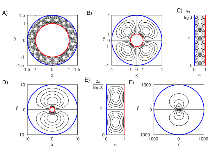
Figure 2: Streamlines for optimal convection cooling flows in annular domains, with the outer (cold) boundary at different radii $R$ = 1.5 (A), 4 (B), 10 (D), and 1000 (F). The inner (hot) boundary has radius 1. Panels C and E show the flows in panels B and D in $(\alpha,\beta)$ coordinates. The streamlines are plotted without arrows because there is no change in the heat transferred when the flow direction is reversed. The streamlines are plotted at nine equally spaced values between the extrema of the stream function.

When $R$ is close to 1 (panel A), we have a thin gap between the hot and cold surfaces, and the flows tend to the square convection rolls in a straight channel found by Hassanzadeh et al. (2014). Since $h$ in (14) is $r\log{R}$, which varies little in the thin gap, there is relatively little distortion when the vortices are mapped from the $(\alpha,\beta)$-plane to the $(x,y)$-plane. The case $R\gg 1$ corresponds to the application of the convection cooling of the exterior of a circular body. In this limit (e.g. panel F), the optimal flow is

$$\psi_{max}=-A_{11}\sin{\left(\pi\left(1-\frac{\log{r}}{\log{R}}\right)\right)}\sin(\theta).$$ (38)

which consists of a pair of oppositely-signed vortices forming a dipole near the body. The amount of vortex distortion is given by $h=r\log{R}$, so the vortices are strongly stretched moving outward from the body. The centers of the vortices are located at $r=\sqrt{R}$, the local extrema of $\psi_{max}$. Differentiating (38) with respect to $r$, we find that the azimuthal flow speed $u_{\theta}$ is proportional to $1/r$ in the neighborhood of the body ($1\leq r\ll R$). When $\Delta\beta/2=\pi/\log{R}$ is an integer, $Q_{2,max}=1/4\pi^{2}$. For large $R$, $Q_{2,max}$ is attained with $n=k=1$. Consequently, with a fixed total kinetic energy, the optimal heat transferred by convection ($Pe^{2}Q_{2,max}\sim Pe^{2}\log^{-2}{R}$) decays slowly as the outer radius increases. Physically, it seems reasonable that the optimal heat transferred with fixed kinetic energy should decrease as the hot and cold surfaces become more distant.

We have discussed optimal convection cooling using the specific example of an annular geometry, but similar results can be obtained for a wide range of geometries. The first step is to compute $(\alpha,\beta)$ for a given geometry. In the next two sections we discuss the solutions for two geometries which are relevant to applications. We find that a slight modification is needed in cases where the hot and cold surfaces meet.

3 Hot plate embedded in a cold surface

The next geometry we consider is a hot plate embedded in a cold surface (see figure 3). The hot plate gives a simple model of a flat heated surface such as a computer processor. An important difference with the previous case is that the cold and hot surfaces are now connected (or nearly so, as we will discuss). We nondimensionalize by the length of the plate.

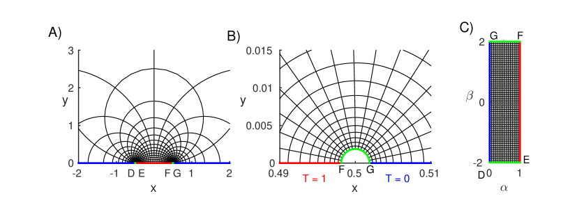
Figure 3: A) A portion of the flow domain–the upper half plane–near the hot boundary. The hot boundary extends nearly to the limits of the interval ($|x|\leq 1/2,y=0$). The cold boundaries are approximately ($|x|>1/2,y=0$). They are joined by small insulating boundaries which are approximately semi-circular. The curvilinear grid plots equicontours of the conformal coordinates $\alpha=\frac{1}{\pi}\left(\arg{\left(z-\frac{1}{2}\right)}-\arg{\left(z+\frac{1}{2}\right)}\right)$ and $\beta=-\frac{1}{\pi}\log{\left|\frac{z-1/2}{z+1/2}\right|}$. B) Close-up near $z=1/2$. The approximate semi-circle closest to 1/2 (light grey or green) is the contour $\beta=2$. This is one of the insulating boundaries of the truncated domain, with the other located near $z=-1/2$. C) The flow domain in ($\alpha,\beta$) space. The letters D, E, F, G show corresponding points in panels A) and B).

The plate (where $T=1$) occupies $-1/2\leq x\leq 1/2$ on the real axis, and the cold surface (where $T=0$) is $|x|>1/2$. The fluid lies in the upper half plane $y>0$. In terms of the complex coordinate $z=x+iy$, the pure conduction solution (with $Pe$ = 0) is

$$T_{0}=\frac{1}{\pi}\left(\arg{\left(z-\frac{1}{2}\right)}-\arg{\left(z+\frac{1}{2}\right)}\right).$$ (39)

Following the same procedure as before,

$$\alpha=\frac{1}{\pi}\left(\arg{\left(z-\frac{1}{2}\right)}-\arg{\left(z+\frac{1}{2}\right)}\right),\quad\beta=-\frac{1}{\pi}\log{\left|\frac{z-1/2}{z+1/2}\right|}$$ (40)

These are also known as bipolar coordinates, with foci at $x=\pm 1/2$. In these coordinates, the flow domain is $0<\alpha<1$, $-\infty<\beta<\infty$. The problem is no longer periodic in $\beta$, and new boundary conditions are required at $\beta=\pm\infty$. To proceed, we first truncate the domain to $0<\alpha<1$, $\beta_{min}<\beta<\beta_{max}$, introducing new boundaries at finite values $\beta_{min}<0$ and $\beta_{max}>0$. By (40), the boundaries’ distances from $z=\pm 1/2$ decay exponentially fast ($\sim e^{-|\beta_{min}|\pi}$, $e^{-|\beta_{max}|\pi}$) as $\beta_{min}$ and $\beta_{max}$ grow in magnitude. Therefore with moderate values of $\beta_{min}$ and $\beta_{max}$ we obtain a good approximation to the original non-truncated domain in the $(x,y)$ plane.

We find that the leading-order solution for $T$ is still $T_{0}$ if we make the new boundaries insulating, so $0=\partial_{n}T=\partial_{\beta}T/h$. $T_{0}$ satisfies this boundary condition because $\partial_{\beta}T_{0}=\partial_{\beta}\alpha=0$ ($\alpha$ and $\beta$ are orthogonal coordinates). Recomputing the variation of $\mathcal{L}$ with these Neumann (instead of periodic) conditions at the $\beta$ boundaries, we find that $m$ has the same boundary conditions as $T$, and thus as before, $m_{0}=T_{0}$, $m_{1}=-T_{1}$. We assume the insulating boundaries are solid walls that the flow does not penetrate. Because they are connected to the hot and cold boundaries, this requires $\psi=0$ on all four sides of the rectangular domain in $(\alpha,\beta)$ space. Thus we obtain the same eigenvalue problem as (29)–(31) but with $\partial_{n}T_{1}=\psi_{1}=0$ on the insulating sides of the rectangle. The eigenfunctions are slightly modified from (32)–(33):

$$\psi_{1} =A_{kn}\sin(k\pi\alpha)\sin(\pi n(\beta-\beta_{min})/\Delta\beta),$$ (41)

$$T_{1} =B_{kn}\sin(k\pi\alpha)\cos(\pi n(\beta-\beta_{min})/\Delta\beta)$$ (42)

with

$$A_{kn} =\left(\frac{1/\Delta\beta}{(\pi k)^{2}+(\pi n/\Delta\beta)^{2}}\right)^{1/2},$$ (43)

$$B_{kn} =\frac{-(1/\Delta\beta)^{1/2}(\pi n/\Delta\beta)}{\left[(\pi k)^{2}+(\pi n/\Delta\beta)^{2}\right]^{3/2}},$$ (44)

$$\lambda =\frac{-(\pi n/\Delta\beta)^{2}}{\left[(\pi k)^{2}+(\pi n/\Delta\beta)^{2}\right]^{2}}.$$ (45)

Because the Neumann boundaries are solid insulating walls, (17) still holds, and $Q_{2}$, the leading contribution to the heat transferred by a given mode, is

$$Q_{2}=-\lambda=\frac{(\pi n/\Delta\beta)^{2}}{\left[(\pi k)^{2}+(\pi n/\Delta\beta)^{2}\right]^{2}}.$$ (46)

$Q_{2}$ is maximized when $k=1$ and $n$ is one of the two integers closest to $\Delta\beta$, which again results in convection rolls which are square (or nearly so, if $\Delta\beta$ is not an integer) in $(\alpha,\beta)$ space. In figure 4 we show examples of optimal flows when $\Delta\beta$ is even (panel A) and odd (panels C and F).

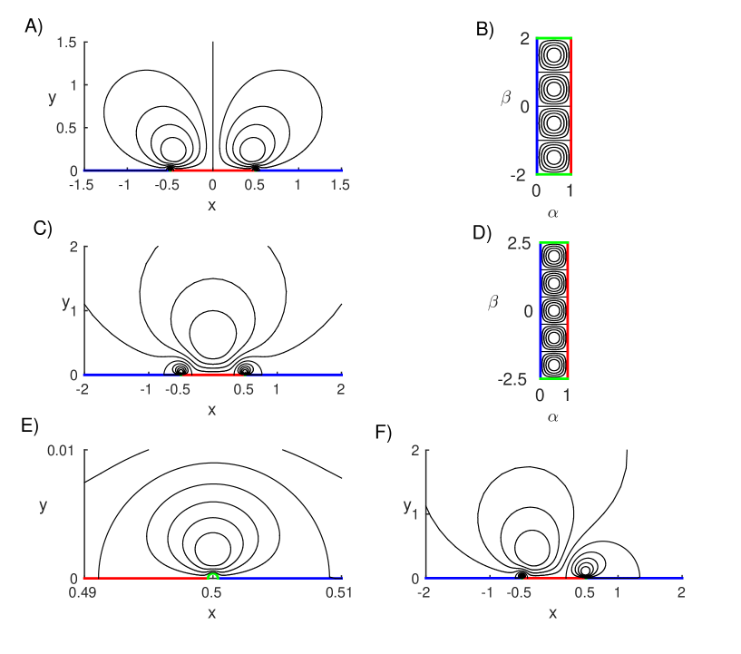
Figure 4: A) Optimal heat transferring flow with $\beta_{min}$ = -2 and $\beta_{max}$ = 2. The flow has four vortices: one pair of large vortices of the order of the plate length, and one pair of small vortices of the order of the insulating boundary length. B) Flow from panel A in $(\alpha,\beta)$ coordinates. C) Optimal heat transferring flow with $\beta_{min}$ = -2.5 and $\beta_{max}$ = 2.5. The flow has five vortices, one large vortex centered over the plate and two pairs symmetric about the y-axis. D) Flow from panel C in $(\alpha,\beta)$ coordinates. E) Close-up of the flow in panel C near $z=1/2$, showing one of the smaller vortices, near the insulated boundary (light gray or green). F) Example of an asymmetric flow with $\beta_{min}=-2.75$, $\beta_{max}=2.25$. Five vortices are present, and the two nearest the insulated boundaries are too small to be visible.

We have a chain of vortices which are $O(1)$ in size above the hot plate, and shrink exponentially in size as they approach the insulated boundaries at the hot-cold interface. In panel A, $\beta_{min}$ = -2 and $\beta_{max}$ = 2, and there are four vortices, one large pair and one small pair. The smallest vortices are proportional in size to the insulated boundaries. Panel B shows the same flow in the $(\alpha,\beta)$ plane. Panel C shows the optimal flow with $\beta_{min}$ = -2.5 and $\beta_{max}$ = 2.5, so there are five vortices (the smallest pair is not visible). Panel D shows this flow in the $(\alpha,\beta)$ plane. Panel E shows the flow near one of the small vortices in panel C at the insulated boundary near $z=1/2$. Panel F shows an asymmetric case, $\beta_{min}$ = -2.75 and $\beta_{max}$ = 2.25. Again there are five vortices, but now they are asymmetric with respect to the plate center. The size of each vortex is proportional to its distance from the insulated boundary, and the typical flow speed within each vortex is inversely proportional to its typical length. Therefore, as the vortices become smaller, the flow speed increases such that the total kinetic energy of each vortex (proportional to its area times typical flow speed squared) is constant.

Once again, $Q_{2,max}=1/4\pi^{2}$ (when $\Delta\beta$ is an integer), so the optimal heat transferred by convection is essentially the same when we vary the positions of the insulating boundaries. The optimal flow varies considerably with the positions of the insulating boundaries, however, because they set the vortices’ positions. It is somewhat surprising that the optimal heat transferred by convection does not increase as the hot and cold surfaces are brought together (for the annulus we found a slow decrease in the heat transferred, but only when the surfaces are very distant). However, the heat transferred by conduction ($\Delta\beta$) diverges logarithmically as the distance between the hot and cold surfaces tends to zero.

4 Channel with hot interior and cold exterior

A classic configuration for heat transfer is the flow through a heated channel (Eagle & Ferguson (1930); Dipprey & Sabersky (1963); Bird et al. (2007); Lienhard (2013); Bejan (2013)). Recent works have studied the dynamics of flapping flags and vortex streets in channels (Alben (2015); Wang & Alben (2015)) with the goal of improving heat transfer efficiency by using vortices to mix the temperature field (Gerty (2008); Shoele & Mittal (2014); Jha et al. (2015)). Here we consider a heated channel in an unbounded fluid (figure 5A).

Figure 5: A) Heated channel in an unbounded flow domain. The inside surfaces of the channel walls have temperature $T=1$ and outside surfaces have $T=0$. B) The flow domain in $\alpha,\beta$ space for the case $L=2,\beta_{min}=-0.5,$ and $\beta_{max}=0.5$. The light blue (light gray) dot marks the point at infinity and the black triangle marks the origin in $x,y$ space. The green boundaries are insulated surfaces, and the red and blue boundaries are the hot and cold surfaces of the upper channel wall. C) The upper half of the flow domain in $x,y$ space. The red, blue, green, and yellow lines and triangle correspond to those in panel B. The curvilinear grid plots equicontours of $\alpha$ and $\beta$.

The inside surfaces of the channel walls are fixed at temperature $T=1$ and the outside surfaces are fixed at $T=0$. If we assume that the channel flow is a perturbation of unidirectional flow, we could possibly truncate the fluid domain to the interior of the channel, and use inflow and outflow boundary conditions for the fluid and temperature (Shoele & Mittal (2014); Wang & Alben (2015)). However, we wish to make minimal assumptions about the flow and therefore we represent the flow both inside and outside the channel. Energy is needed to drive the flow through the entire fluid domain, so it makes sense to include the outside flow in the optimization calculation.

The analytic function $\alpha+i\beta$ can be found numerically by using complex analysis and boundary integral methods. Because $T$ (and therefore $\alpha$) has a jump across the channel walls, we can use the Plemelj formula (Estrada & Kanwal (2012)) to write $\alpha+i\beta$ in the form

$$\alpha(z)+i\beta(z)=\frac{1}{2\pi i}\int_{C}\frac{\gamma(s)+i\eta(s)}{z-\zeta(s)}ds+C_{1}$$ (47)

where $C$ is a complex contour parametrized by arc length as $\zeta(s)$, representing the union of the two channel walls, $s\pm i/2,-L/2<s<L/2$. The real constant $C_{1}$ will be chosen shortly. The function $\gamma(s)+i\eta(s)$ corresponds to the jump in $\alpha(s)+i\beta(s)$ along the contour. From the boundary conditions on $\alpha$ (those of $T$) we have $\gamma(s)=\pm 1$ on $\zeta(s)=s\pm i/2$. It remains to find $\eta(s)$. We note that (47) provides the average value of $\alpha+i\beta$ on the countour when $z$ is a point on the contour and the integral is changed from an ordinary integral to a principal value integral. We solve for $\eta(s)$ by the condition that the average value of $\alpha(s)$ on the contour equals $1/2$:

$$1/2=Re\left[\frac{1}{2\pi i}~{}-\int_{-L/2}^{L/2}\left(\frac{1+i\eta(s)}{s^{\prime}-s}+\frac{-1+i\eta(s)}{s^{\prime}-s+i}\right)\,ds\right]+C_{1},\;\;-L/2<s^{\prime}<L/2.$$ (48)

We have written the contributions from the two channel walls in (47) separately and used symmetry considerations to deduce that $\eta$ on the lower wall equals that on the upper wall. We use the Chebyshev collocation method (Golberg (1990)) to solve (48) with $s$ at points on a Chebyshev-Lobatto grid and $s^{\prime}$ on a Chebyshev-Gauss grid. We need two additional constraints to uniquely specify $\eta$ and $C_{1}$ in (48) (Golberg (1990)). These can be given as:

$$\lim_{s\rightarrow\pm L/2}\eta(s)\sqrt{L^{2}/4-s^{2}}=0.$$ (49)

These conditions are preferred because they make $\eta$ a bounded continuous function. Having solved for $\eta$ and $C_{1}$ and knowing $\gamma$, we evaluate $\alpha$ and $\beta$ using (47). As with the single heated plate, we find that $\beta\rightarrow\pm\infty$ at the plate edges where the hot and cold boundaries meet. So as before, we cut off the domain with small insulated boundaries at $\beta=\beta_{min}$ and $\beta_{max}$. In figure 5B and C we show $(\alpha,\beta)$ equicontours and their location in the $(x,y)$ plane, respectively, for the case $L=2$. Here we use $\beta_{min}=-0.5,\beta_{max}=0.5$. These values are relatively small in magnitude so that the insulated boundaries are large enough to be clearly visible. As with the single heated plate example, the insulated boundaries approach the plate edges exponentially with increasing magnitude of these values.

In panel C, we show only the upper half plane in $(x,y)$. In the lower half plane, the values of $\alpha$ and $\beta$ can be smoothly continued from the upper half plane, by reflecting the values in the origin. Thus the flow is also smoothly continued in the lower half-plane by reflecting $\psi$ in the origin.

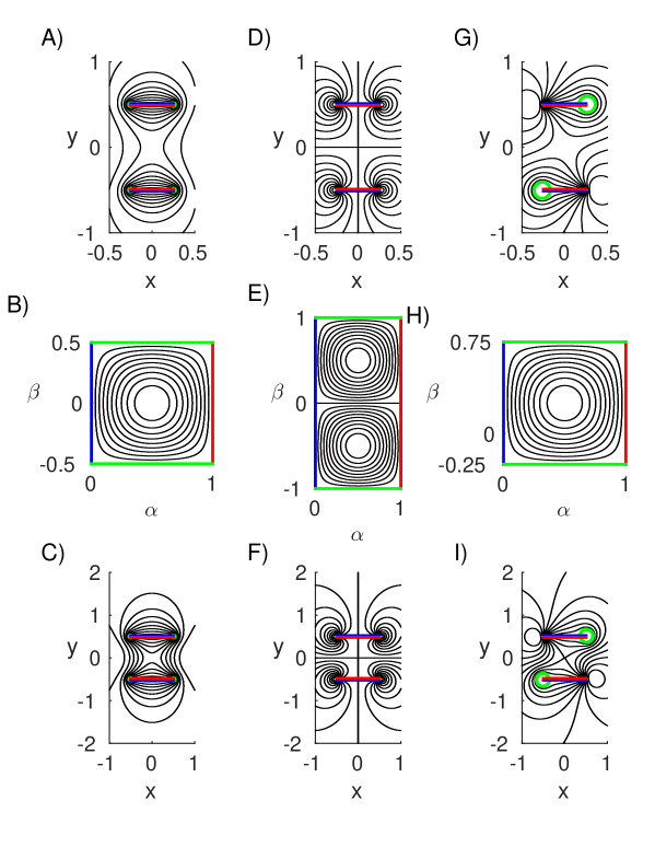
Figure 6: Streamlines of optimal heat transferring flows for short channels. The channel lengths are $L=0.5$ in the top row (A, D, G) and 1 in the bottom row (D, F, I). The middle row (B, E, H) shows the flows from the top and bottom rows in $(\alpha,\beta)$ coordinates, where they are the same. Moving from left to right, the positions of the insulated boundaries (green) varies: $\beta_{min}=-0.5,$ and $\beta_{max}=0.5$ (A-C), $\beta_{min}=-1,$ and $\beta_{max}=1$ (D-F, too close to the plate edges to be visible), and $\beta_{min}=-0.25,$ and $\beta_{max}=0.75$ (G-I).

In figure 6 we show optimal flows for “short” channels, with lengths less than or equal to the channel height. The top row (A, D, G) shows optimal flows when the channel length is half the height. The only difference between A, D, and G is the location of the insulating boundaries. As we have seen with the single plate, this makes a big difference in the optimal flow. In panel A, the flow consists of rolls that move around the plates. There is a strong net flow through the channel, which is fast near the channel walls, and slow in the middle of the channel. The corresponding flow in the $(\alpha,\beta)$ plane is shown in panel B. It is a single vortex which is mapped twice onto the $(x,y)$ plane in panel A by reflection in the origin, as mentioned previously. In panel D we move the insulating boundaries closer to the plate edges, and obtain two pairs of vortices moving around the edges of the channel. The flow is fastest near the plate edges, where the hot and cold surfaces are closest. Panel E shows the corresponding flow in the $(\alpha,\beta)$ plane. Panel G shows an example in which the insulating boundaries are asymmetric in $\beta$, with the $(\alpha,\beta)$ representation shown in panel H.

The bottom row (C, F, I) shows optimal flows when the channel length equals its height. The corresponding flows in the $(\alpha,\beta)$ plane are again those in panels B, E, and H. In panel C, the flow has a stronger circulatory component that moves across the channel openings, from top to bottom and vice versa, around the outside of the entire channel, compared to that in panel A. In panels F and I, the flow is also stronger near the centers of the channel openings than in the corresponding flows of the top row (D and G).

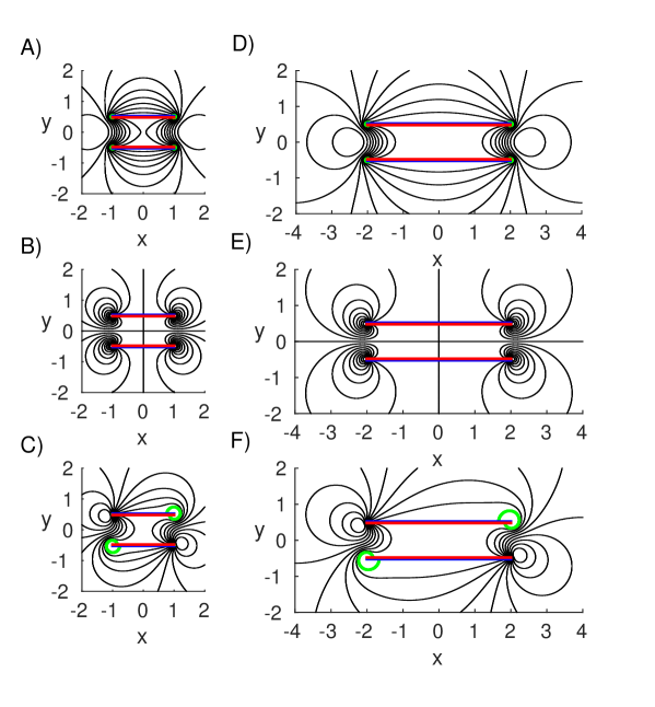
Figure 7: Streamlines of optimal heat transferring flows for longer channels (lengths $L=2$ (A-C) and 4 (D-F) in units of channel width). For the length-2 channels (A-F), the insulated boundaries (green) are located at A) $\beta_{min}=-0.5,$ and $\beta_{max}=0.5$, B) $\beta_{min}=-1,$ and $\beta_{max}=1$ (too close to the plate edges to be visible), and C) $\beta_{min}=-0.25,$ and $\beta_{max}=0.75$. For length-4 channels (D-F), the insulated boundaries (green) are located at D) $\beta_{min}=-0.5,$ and $\beta_{max}=0.5$, E) $\beta_{min}=-1,$ and $\beta_{max}=1$ (too close to the plate edges to be visible), and F) $\beta_{min}=-0.25,$ and $\beta_{max}=0.75$.

In figure 7 we show optimal flows when the channel length is increased to two (A-C) and four (D-F) times the channel height. Now the flows are strongly confined to the channel openings. There is very little flow in the center of the channel. The reason is that the temperature due to pure conduction ($T_{0}=\alpha$) is nearly uniform in the center of the channel. There is little to be gained by using energy to transport fluid through this region of nearly uniform temperature. Since $\alpha$ changes little in this region, $h=\|\partial\mathbf{X}/\partial\alpha\|=\|\partial\mathbf{X}/\partial\beta\|\gg 1$ and the flow speed $\|\mathbf{u}\|=\|-\nabla^{\perp}_{x,y}\psi\|=\|-\nabla^{\perp}_{\alpha,\beta}\psi/h\|\sim 1/h\ll 1.$ The lack of flow through the channel is a significant difference from typical channel convection cooling flows (Bird et al. (2007)). This can be attributed to our objective of maximizing the total heat flux out of the hot walls. In these solutions, most of the flux is close to the channel openings, near the cold exterior.

5 Large amplitude flows

We now consider the case where $Pe$ is not small by returning to equations (9)–(12), which hold for all $Pe\geq 0$. We have noted that this is the same as the constant-kinetic-energy problem considered by Hassanzadeh et al. (2014) under the transformation $(\alpha,\beta)\rightarrow(1-z,x)$. They computed numerically the solutions from $Pe$ small to large and derived a boundary layer solution for the optimal flow in the limit of large $Pe$. Their derivation works for both the periodic and Neumann boundary conditions (in $\beta$) that we used here. We simply translate the complete asymptotic solution for $\psi$ that they found into an $(\alpha,\beta)$ rectangle with $\beta$-width $\Delta\beta$:

$$\psi \sim\frac{f(\mu_{H},\Gamma)}{\sqrt{2\mu_{H}}}\sin\left(\frac{N\pi(\beta-\beta_{min})}{\Delta\beta}\right)\tanh\left(\frac{\pi f(\mu_{H},\Gamma)(1-\alpha)}{2\sqrt{2\mu_{H}}\,\Gamma}\right)\tanh\left(\frac{\pi f(\mu_{H},\Gamma)\alpha}{2\sqrt{2\mu_{H}}\,\Gamma}\right)$$

$$\mbox{where}\quad f(\mu_{H},\Gamma)=1-\frac{\pi\sqrt{2\mu_{H}}}{2\Gamma}.$$ (50)

In the limit of large $Pe$, equal-aspect-ratio convection rolls are no longer optimal. Instead, the convection rolls become very narrow in the $\beta$ direction, with narrow boundary layers of fast-moving fluid along the hot and cold walls. The size of the boundary layers and the $\beta$-width of the rolls are set by the parameters $\Gamma$ and $\mu_{H}$ (= $2\lambda$) in (50). For $Pe\gg 1$ Hassanzadeh et al. (2014) found that for the optimal rolls,

$$\Gamma\sim 3.8476Pe^{-1/2}\Delta\beta^{1/4}\quad;\quad\mu_{H}=\Gamma^{2}/8\pi^{2},$$ (51)

where we have added the $\Delta\beta$ term due to our different definition of $Pe$. This solution is valid for our problems with Neumann conditions at the $\beta$ boundaries when $\Delta\beta/\Gamma$ is an integer, $N$ in (50). For periodic boundary conditions, $N$ must be even.

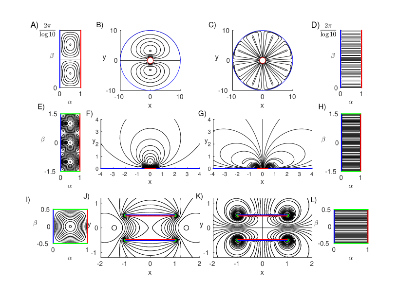
Figure 8: A comparison of optimal flows with small and large kinetic energy ($Pe$) across the three geometries considered in this work. Top row (A-D): optimal flows in an annulus with outer radius $R=10$. A) Small-$Pe$ optimal flow in $(\alpha,\beta)$. B) Small-$Pe$ optimal flow in $(x,y)$. C) Large-$Pe$ ($Pe\approx$ 210) optimal flow in $(x,y)$. D) Large-$Pe$ ($Pe\approx$ 210) optimal flow in $(\alpha,\beta)$. Middle row (E-H): optimal flows over a hot plate in a cold surface. E) Small-$Pe$ optimal flow in $(\alpha,\beta)$. F) Small-$Pe$ optimal flow in $(x,y)$. G) Large-$Pe$ ($Pe\approx$ 182) optimal flow in $(x,y)$. H) Large-$Pe$ ($Pe\approx$ 182) optimal flow in $(\alpha,\beta)$. Bottom row (I-L): optimal flows around a channel with hot interior and cold exterior. I) Small-$Pe$ optimal flow in $(\alpha,\beta)$. J) Small-$Pe$ optimal flow in $(x,y)$. K) Large-$Pe$ ($Pe\approx$ 237) optimal flow in $(x,y)$. L) Large-$Pe$ ($Pe\approx$ 237) optimal flow in $(\alpha,\beta)$.

In figure 8 we plot a few examples of optimal flows at moderately large $Pe$ for the geometries we have considered, together with the corresponding small-$Pe$ optima. The top row shows flows past a cylinder with outer boundary at $R=10$ at small $Pe$ in $(\alpha,\beta)$ (A) and $(x,y)$ (B), the same flows as in figure 2E and D, respectively. The large-$Pe$ optimum is shown in panels C and D of figure 8. $Pe\approx 210$ so that $N=8$. The streamlines are approximately rectangles in $(\alpha,\beta)$ (D), which map onto approximate wedges in $(x,y)$ (C). In the middle row, we show optimal flows over a hot plate at small $Pe$ (E, F, similar to those in figure 4) and $Pe\approx 182$ (G, H). A given rectangular streamline in $(\alpha,\beta)$ (H) maps onto a streamline which approximately follows one larger circle and one smaller circle (in the opposite direction) in the bipolar coordinate system (figure 3A) connected by segments along the hot and cold plates. In the bottom row, optimal flows in a channel of length 2 are shown at small $Pe$ (I, J) and $Pe\approx 237$ (K, L), giving $N=4$. In this case a rectangular streamline in $(\alpha,\beta)$ maps onto a streamline which follows two arcs which are roughly circles centered at the channel edges. The arcs are again connected by segments along the hot and cold plates.

6 More general geometries

We have studied three examples which are representative of a more general class of problems which can be solved with the same method. The main step is to solve for $(\alpha(x,y),\beta(x,y))$. The first case, flow through an annulus, can be extended to any doubly connected region which lies between one simple closed curve on which the temperature is 1 and another on which the temperature is 0. The flow region may include the point at infinity. All such regions correspond to a rectangle in $(\alpha,\beta)$ space on which the boundary conditions for $\psi$ and $T$ are Dirichlet on the $\alpha=0$, $\alpha=1$ sides and periodic on the $\beta=\beta_{min}$, $\beta=\beta_{max}$ sides.

The second case, flow over a heated plate, can be generalized to the flow within any region bounded by a simple closed curve which is partitioned into four arcs. On the four arcs the boundary conditions are $T=0$, $\partial_{n}T=0$, $T=1$, and $\partial_{n}T=0$, moving continuously around the curve. On the entire curve $\psi=0$. The curve may include the point at infinity (as for the heated plate), and in general we may use any simple closed curve on the Riemann sphere. On the arcs where $\partial_{n}T=0$, we have $0=\partial_{n}T_{0}=\partial_{n}\alpha=-\partial_{s}\beta$, so $\beta$ is constant. All such cases correspond to a rectangle in $(\alpha,\beta)$ space on which the boundary conditions are Dirichlet for $\psi$, and Dirichlet and Neumann for $T$ on the $\alpha$ and $\beta$ sides, respectively. The green arcs in figures 3-7 were chosen because they followed lines of constant $\beta$ for functions which could be written in closed form or computed relatively easily, but the shapes of the insulated boundaries can be arbitrary in general.

The third case, flow through a heated channel, is an example where the flow lies in the region between two simple closed curves, each of which is partitioned into four arcs as above. Here by symmetry the same rectangle in $(\alpha,\beta)$ was used to cover the $(x,y)$ space twice. This case can be generalized to nonsymmetrical configurations of $n$ closed curves, and the curves may contain multiple arcs on which $T=0$ and $T=1$.

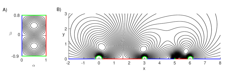
Figure 9: Optimal small kinetic energy flow (small $Pe$) over a surface with two hot plates (red) separated by cold plates (blue) and insulated boundaries (green), in $(\alpha,\beta)$ (A) and $(x,y)$ (B). The flow is described by (41) with $\beta_{min}=-0.9$, $\beta_{max}=0.8$, and ($\alpha,\beta$) given by (52).

Figure 9 shows an example where the flow domain is the upper half plane, bounded by two hot and three cold segments along the $x$ axis. On the Riemann sphere this is one closed curve on which the temperature is 1 on two arcs and 0 on two arcs. Here

$$\alpha=\frac{1}{\pi}\arg{\left(\frac{(z-6)(z-3)}{(z-5)z}\right)},\quad\beta=-\frac{1}{\pi}\log{\left|\frac{(z-6)(z-3)}{(z-5)z}\right|}.$$ (52)

The rectangle with sides $\alpha=0$, $\alpha=1$, $\beta=-0.9$, $\beta=0.8$ maps twice onto the flow region. Moving around the rectangle counterclockwise twice in panel A corresponds to moving along the boundary on the $x$ axis and green arcs in panel B from $x=-\infty$ to $+\infty$. In the small-$Pe$ limit the stream function is (41) with $n=2$.

7 Fixed enstrophy flows

Hassanzadeh et al. (2014) also considered the optimization problem with fixed enstropy instead of fixed kinetic energy. Fixed enstropy is equivalent to a fixed rate of viscous energy dissipation, which is proportional to the enstrophy for our flow boundary conditions (solid walls or periodic boundaries) (Lamb (1932)). In place of (6) we have:

$$\frac{1}{2}\iint\nabla\mathbf{u}:\nabla\mathbf{u}\,dA=\iint(\Delta\psi)^{2}dA=Pe^{2}.$$ (53)

Here $Pe=\sqrt{\dot{E}/\mu W}$ is redefined to include the (steady) total rate of viscous energy dissipation $\dot{E}$ instead of the total kinetic energy, the fluid viscosity $\mu$, and the out-of-plane width $W$. With (53) instead of (6) in the Lagrangian (8), the equation for $\psi$ becomes

$$0=-\nabla^{\perp}T\cdot\nabla m-2\lambda\Delta^{2}\psi\quad,\quad\psi=\mbox{const.},\;\partial_{n}\psi=0\;\mbox{on boundaries}.$$ (54)

instead of (11); (54) includes the biharmonic operator and therefore an additional boundary condition on $\psi$, the no-slip condition corresponding to a viscous flow. In $(\alpha,\beta)$ coordinates, (53) becomes

$$\iint\frac{1}{h^{2}}(\Delta_{\alpha,\beta}\psi)^{2}dA_{\alpha,\beta}=Pe^{2}.$$ (55)

and (54) becomes

$$0=-\nabla_{\alpha,\beta}^{\perp}T\cdot\nabla_{\alpha,\beta}m-2\lambda\Delta_{\alpha,\beta}\left(\frac{1}{h^{2}}\Delta_{\alpha,\beta}\psi\right),\quad\psi=\mbox{const.},\;\partial_{n}\psi=0\;\mbox{on boundaries}.$$ (56)

The metric term ($1/h^{2}$) in (56) is a function of $(\alpha,\beta)$ given by (14), different for each geometry, and therefore unlike for the fixed kinetic energy case, the solutions are not geometry-independent when viewed in $(\alpha,\beta)$ coordinates.

The case of a straight channel between hot and cold walls (where $h\equiv 1$) was solved by Hassanzadeh et al. (2014) with free-slip boundary conditions instead of no-slip conditions, to simplify the problem. In this case, for small $Pe$ the optimal flows are sinuosoidal convection rolls with the same form as for the fixed kinetic energy case, but with a different aspect ratio ($\sqrt{2}$ versus 1). At large $Pe$, the boundary layer structure is different, but the outer flow has the same form as in the fixed kinetic energy case. In the no-slip case, the optimal flows with fixed enstrophy were computed numerically by Souza (2016) and compared to the free-slip case. The solutions are similar qualitatively in both cases at small and large $Pe$. In both cases there is a transition from convection rolls with “round” streamlines and a moderate aspect ratio at small $Pe$ to narrow rectangular convection rolls at large $Pe$. At large $Pe$ there are significant differences in the boundary layer structure, and a small difference in the power-law scaling of heat transferred ($Q$) with respect to $Pe$: $Q\sim Pe^{0.58}$ for the stress-free optima while $Q\sim Pe^{0.54}$ for the no-slip optima.

For more general geometries, the fixed-enstrophy problem requires a numerical solution. The $(\alpha,\beta)$ coordinates are useful here because they map the flow domain onto a rectangle, where the differential operators can be discretized by finite differences on uniform grids. The ($1/h^{2}$) factor in (55) can be viewed as a weight that decreases the cost of vorticity where $h$ is large. By (14), $h=\|\partial_{x}\alpha,\partial_{y}\alpha\|^{-1}=\|\nabla T_{0}\|^{-1}$, so the cost of vorticity is decreased where $\|\nabla T_{0}\|$ is small. Typically this occurs far from the hot surface.

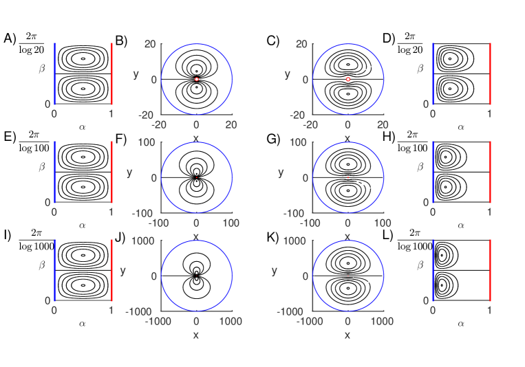
Figure 10: Comparison of small-$Pe$ optimal flows in an annulus with fixed kinetic energy (left two columns) and fixed enstrophy (right two columns). The outer boundary radius is $R$ = 20 (top row, A-D), 100 (middle row, E-H), and 1000 (bottom row, I-L). The fixed kinetic energy flows are shown in the first column (A, E, I) in the $(\alpha,\beta)$ plane and in the second column (B, F, J) in the $(x,y)$ plane. The fixed-enstrophy flows are shown in the third column (C, G, K) in the $(x,y)$ plane and in the fourth column (D, H, L) in the $(\alpha,\beta)$ plane.

We now discuss the solutions to the small-$Pe$ eigenvalue problem with fixed enstrophy for the annular domains with various outer radii $R$. In the third column of figure 10 we present the optimal flows at $R$ = 20 (C), 100 (G), and 1000 (K) in the $(x,y)$ plane. When lengths are scaled by $R$, the flows converge to a common solution in the large-$R$ limit, consisting of a smooth vortex dipole which is the size of the domain (and obeys no-slip at the boundaries). In the fourth column, the same flows are shown in the $(\alpha,\beta)$ plane. As $R$ increases (moving from panel D to H to L), the vorticity moves towards $\alpha=0$, where $h=R^{1-\alpha}\log(R)$ is largest. In the second column (B, F, J) we plot the optimal flows with fixed kinetic energy. In these cases the vortex dipole is stretched towards the inner cylinder, with each vortex center at a distance $\sim\sqrt{R}$ from the origin. In the first column, the same flows are shown in the $(\alpha,\beta)$ plane, where they become identical under a rescaling of the $\beta$ axis.

With fixed kinetic energy, we have larger vorticity near the inner cylinder. This vorticity is spread more uniformly in the fixed-enstrophy solutions. We now show that for these flows (i.e. panels C, G, and K), the kinetic energy diverges in the limit of large $R$. For the fixed-enstrophy flows, we have $\iint(\Delta_{x,y}\psi)^{2}dA=Pe^{2}$. Thus $(\Delta_{x,y}\psi)^{2}R^{2}\sim Pe^{2}$ so $Pe/R\sim\Delta_{x,y}\psi\sim\psi/R^{2}$. Thus $\psi\sim R$ and $\mathbf{u}=-\nabla_{x,y}^{\perp}\psi\sim\mathbf{1}$. Thus the flow speed is of order 1 over an area $\sim R^{2}$, so the kinetic energy diverges as $R^{2}$ as $R$ becomes large.

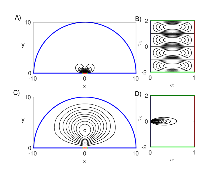
Figure 11: Comparison of small-$Pe$ optimal flows with fixed kinetic energy (top row) and fixed enstrophy (bottom row) in a half-disk with radius 10 above a heated plate of unit length centered at the origin. Optimal flow with fixed kinetic energy in the $(x,y)$ plane (A) and the $(\alpha,\beta)$ plane (B). Optimal flow with fixed enstrophy in the $(x,y)$ plane (C) and the $(\alpha,\beta)$ plane (D). Here we use $\beta_{min}=-2$, $\beta_{max}=2$.

For the optimal flow over a heated plate in section 3, the domain is infinite. We have $h=\frac{\pi}{2}\left(\cosh(\pi\beta)-\cos(\pi\alpha)\right)^{-1}$. As $(\alpha,\beta)\to(0,0)$, $h\sim\|(\alpha,\beta)\|^{-2}$. Thus the small-$Pe$ eigenvalue problem is singular. Solving the problem numerically in the $(\alpha,\beta)$ rectangle, we find that the solutions have infinite kinetic energy and do not satisfy $\psi\to 0$ as $(\alpha,\beta)\to(0,0)$ (or $x+iy\to\infty$). To examine the situation further, we consider a regularized version of the problem, in which the domain is cut off by a large semi-circle of radius $R$ on which $T=0$ (see figure 11A). We compute $\alpha$ and $\beta$ for this domain by modifying the unbounded definition (40):

$$\alpha+i\beta=\frac{-i}{\pi}\log{\left(\frac{z-1/2}{z+1/2}\right)}-i\sum_{k=1}^{\infty}a_{k}z^{k}.$$ (57)

We have added a power series, which gives a general representation of an analytic function which converges inside the disk of radius $R$. We truncate the series at $k=N$ and choose the $a_{k}$ so that the $\sin{k\theta}$-components of $\alpha$ are zero on $|z|=R$. We find that $a_{k}$ converge rapidly to 0 with increasing $k$, so just a few terms are needed to obtain $\sim 10^{-12}$ precision for $R=10$.

In figure 11 we compare the optimal flows with fixed kinetic energy and enstrophy in the small-$Pe$ limit with $R=10$. The flow with fixed kinetic energy (panel A) is almost identical to that in the unbounded case (figure 4A), because the flow is very weak far from the plate in that case. Panel B shows the same flow in the $(\alpha,\beta)$ plane. The optimal flow with fixed enstrophy (panel C) has a single vortex whose size is roughly that of the domain. Panel D shows this flow in the $(\alpha,\beta)$ plane. The vorticity is concentrated near $(\alpha,\beta)=(0,0)$, where $h$ is largest.

In summary, the optimal flows with fixed enstrophy have vortices which are much larger in scale than those for flows with fixed kinetic energy. In the examples shown here, the fixed-enstrophy flows are of the same size as the physical domain, while the fixed-energy flows are of the order of the size of the hot surface.

8 Summary and possible extensions

We have shown that a certain class of optimal flows for heat transfer can be generalized to a wide range of geometries using a change of coordinates. We presented solutions in three basic situations: the exterior cooling of a cylinder, a hot flat plate embedded in a cold surface, and a channel with hot interior and cold exterior. Steady 2D flows were sufficient to present the basic idea, but unsteady flows can be addressed by retaining the unsteady term in the advection-diffusion equation. It seems likely that the coordinate change would be useful in certain 3D geometries as well, though these problems have not yet been solved.

We acknowledge helpful discussions with Professor Charles R. Doering.

Appendix A Alternative formula for $Q$

Here we show that the two formulas for $Q$, (7) and (17), are equal. Defining the heat flux vector as $\mathbf{q}=\mathbf{u}T-\nabla T=-T\nabla^{\perp}\psi-\nabla T$, equation (9) can be written

$$0=\nabla\cdot\mathbf{q}=\frac{1}{h^{2}}\left[\partial_{\alpha}(h\mathbf{q}\cdot\hat{\mathbf{e}}_{\alpha})+\partial_{\beta}(h\mathbf{q}\cdot\hat{\mathbf{e}}_{\beta})\right].$$ (58)

We integrate over $\beta$:

$$\int_{\beta_{min}}^{\beta_{max}}\partial_{\alpha}(h\mathbf{q}\cdot\hat{\mathbf{e}}_{\alpha})d\beta=-\int_{\beta_{min}}^{\beta_{max}}\partial_{\beta}(h\mathbf{q}\cdot\hat{\mathbf{e}}_{\beta})d\beta=h\mathbf{q}\cdot\hat{\mathbf{e}}_{\beta}|_{\beta_{min}}^{\beta_{max}}=0.$$ (59)

The last equality holds for the annulus because then $\mathbf{q}$ is periodic in $\beta$. The equality also holds for all the other problems in this work, for which the $\beta$ boundaries are solid insulating walls. At such boundaries we have $\mathbf{q}\cdot\hat{\mathbf{e}}_{\beta}=0$. Defining

$$f(\alpha)=-\int_{\beta_{min}}^{\beta_{max}}h\mathbf{q}\cdot\hat{\mathbf{e}}_{\alpha}d\beta$$ (60)

and interchanging the derivative and integral in (59) we have $f^{\prime}(\alpha)=0\Rightarrow f(\alpha)$ = constant. The constant is

$$f(1)=-\int_{\beta_{min}}^{\beta_{max}}h\partial_{n}T|_{\alpha=1}d\beta=-\int_{\alpha=1}\partial_{n}Tds=Q.$$ (61)

using no flow penetration ($\mathbf{u}\cdot\hat{\mathbf{e}}_{\alpha}=0$) along the hot boundary. Because $f(\alpha)$ is constant we also have

$$Q=\int_{0}^{1}f(\alpha)d\alpha=-\int_{0}^{1}\int_{\beta_{min}}^{\beta_{max}}h\mathbf{q}\cdot\hat{\mathbf{e}}_{\alpha}d\beta d\alpha=-\int_{\beta_{min}}^{\beta_{max}}\int_{0}^{1}h\mathbf{q}\cdot\hat{\mathbf{e}}_{\alpha}d\alpha d\beta$$ (62)

Using $\mathbf{q}\cdot\hat{\mathbf{e}}_{\alpha}=u_{\alpha}T-\frac{1}{h}\partial_{\alpha}T$,

$$Q=\Delta\beta-\int_{\beta_{min}}^{\beta_{max}}\int_{0}^{1}hu_{\alpha}Td\alpha d\beta=\Delta\beta-\int_{\beta_{min}}^{\beta_{max}}\int_{0}^{1}\partial_{\beta}\psi\,T\,d\alpha d\beta.$$ (63)

References

- Acheson (1990) Acheson, David J 1990 Elementary fluid dynamics. Oxford University Press.
- Açıkalın et al. (2007) Açıkalın, Tolga, Garimella, Suresh V, Raman, Arvind & Petroski, James 2007 Characterization and optimization of the thermal performance of miniature piezoelectric fans. International Journal of Heat and Fluid Flow 28 (4), 806–820.
- Ahlers (2011) Ahlers, Mark F 2011 Aircraft Thermal Management. Encyclopedia of Aerospace Engineering .
- Alben (2015) Alben, Silas 2015 Flag flutter in inviscid channel flow. Physics of Fluids 27 (3), 033603.
- Bejan (2013) Bejan, Adrian 2013 Convection heat transfer. John Wiley & sons.
- Bird et al. (2007) Bird, R Byron, Stewart, Warren E & Lightfoot, Edwin N 2007 Transport Phenomena. John Wiley & Sons.
- Biswas et al. (1996) Biswas, G, Torii, K, Fujii, D & Nishino, K 1996 Numerical and experimental determination of flow structure and heat transfer effects of longitudinal vortices in a channel flow. International Journal of Heat and Mass Transfer 39 (16), 3441–3451.
- Brown et al. (1996) Brown, James Ward, Churchill, Ruel Vance & Lapidus, Martin 1996 Complex variables and applications, , vol. 7. McGraw-Hill New York.
- Camassa et al. (2016) Camassa, R, Lin, Z, McLaughlin, RM, Mertens, K, Tzou, C, Walsh, J & White, B 2016 Optimal mixing of buoyant jets and plumes in stratified fluids: theory and experiments. Journal of Fluid Mechanics 790, 71–103.
- Campbell et al. (1997) Campbell, MI, Amon, CH & Cagan, J 1997 Optimal three-dimensional placement of heat generating electronic components. Journal of Electronic Packaging 119 (2), 106–113.
- Caulfield & Kerswell (2001) Caulfield, CP & Kerswell, RR 2001 Maximal mixing rate in turbulent stably stratified Couette flow. Physics of Fluids 13 (4), 894–900.
- Chen et al. (2013) Chen, Qun, Liang, Xin-Gang & Guo, Zeng-Yuan 2013 Entransy theory for the optimization of heat transfer–a review and update. International Journal of Heat and Mass Transfer 63, 65–81.
- Chien et al. (1986) Chien, W-L, Rising, H & Ottino, JM 1986 Laminar mixing and chaotic mixing in several cavity flows. Journal of Fluid Mechanics 170, 355–377.
- Da Silva et al. (2004) Da Silva, AK, Lorente, S & Bejan, A 2004 Optimal distribution of discrete heat sources on a wall with natural convection. International Journal of Heat and Mass Transfer 47 (2), 203–214.
- Dipprey & Sabersky (1963) Dipprey, Duane F & Sabersky, Rolf H 1963 Heat and momentum transfer in smooth and rough tubes at various Prandtl numbers. International Journal of Heat and Mass Transfer 6 (5), 329–353.
- Doering et al. (2006) Doering, Charles R, Otto, Felix & Reznikoff, Maria G 2006 Bounds on vertical heat transport for infinite-Prandtl-number Rayleigh–Bénard convection. Journal of fluid mechanics 560, 229–241.
- Eagle & Ferguson (1930) Eagle, Albert & Ferguson, RM 1930 On the coefficient of heat transfer from the internal surface of tube walls. In Proceedings of the Royal Society of London A: Mathematical, Physical and Engineering Sciences, , vol. 127, pp. 540–566. The Royal Society.
- Estrada & Kanwal (2012) Estrada, Ricardo & Kanwal, Ram P 2012 Singular integral equations. Springer.
- Fiebig et al. (1991) Fiebig, Martin, Kallweit, Peter, Mitra, Nimai & Tiggelbeck, Stefan 1991 Heat transfer enhancement and drag by longitudinal vortex generators in channel flow. Experimental Thermal and Fluid Science 4 (1), 103–114.
- Foures et al. (2014) Foures, DPG, Caulfield, CP & Schmid, Peter J 2014 Optimal mixing in two-dimensional plane Poiseuille flow at finite Péclet number. Journal of Fluid Mechanics 748, 241–277.
- Gerty (2008) Gerty, Donavon R 2008 Fluidic driven cooling of electronic hardware. Part I: Channel integrated vibrating reed. Part II: Active heat sink. PhD thesis.
- Golberg (1990) Golberg, MA 1990 Numerical Solution of Integral Equations. Plenum Press.
- Gopinath et al. (2005) Gopinath, Deepak, Joshi, Yogendra & Azarm, Shapour 2005 An integrated methodology for multiobjective optimal component placement and heat sink sizing. Components and Packaging Technologies, IEEE Transactions on 28 (4), 869–876.
- Hassanzadeh et al. (2014) Hassanzadeh, Pedram, Chini, Gregory P & Doering, Charles R 2014 Wall to wall optimal transport. Journal of Fluid Mechanics 751, 627–662.
- Hidalgo et al. (2010) Hidalgo, Pable, Herrault, Florian, Glezer, Ari, Allen, Mark, Kaslusky, Scott & Rock, Brian St 2010 Heat transfer enhancement in high-power heat sinks using active reed technology. In Thermal Investigations of ICs and Systems (THERMINIC), 2010 16th International Workshop on, pp. 1–6. IEEE.
- Jha et al. (2015) Jha, Sourabh, Hidalgo, Pablo & Glezer, Ari 2015 Small-scale vortical motions induced by aeroelastically fluttering reed for enhanced heat transfer in a rectangular channel. Bulletin of the American Physical Society 60.
- Karniadakis (1988) Karniadakis, George EM 1988 Numerical simulation of forced convection heat transfer from a cylinder in crossflow. International Journal of Heat and Mass Transfer 31 (1), 107–118.
- Karniadakis et al. (1988) Karniadakis, George E, Mikic, Bora B & Patera, Anthony T 1988 Minimum-dissipation transport enhancement by flow destabilization: Reynolds’ analogy revisited. Journal of Fluid Mechanics 192, 365–391.
- Kotouč et al. (2008) Kotouč, Miroslav, Bouchet, Gilles & Dušek, Jan 2008 Loss of axisymmetry in the mixed convection, assisting flow past a heated sphere. International Journal of Heat and Mass Transfer 51 (11), 2686–2700.
- Lamb (1932) Lamb, Horace 1932 Hydrodynamics. Cambridge University Press.
- Lienhard (2013) Lienhard, John H 2013 A Heat Transfer Textbook. Courier Corporation.
- McGlen et al. (2004) McGlen, Ryan J, Jachuck, Roshan & Lin, Song 2004 Integrated thermal management techniques for high power electronic devices. Applied thermal engineering 24 (8), 1143–1156.
- Mohammadi et al. (2001) Mohammadi, Bijan, Pironneau, Olivier, Mohammadi, B & Pironneau, Oliver 2001 Applied shape optimization for fluids, , vol. 28. Oxford University Press Oxford.
- Nakayama (1986) Nakayama, Wataru 1986 Thermal management of electronic equipment: a review of technology and research topics. Applied Mechanics Reviews 39 (12), 1847–1868.
- Otero et al. (2004) Otero, Jesse, Dontcheva, Lubomira A, Johnston, Hans, Worthing, Rodney A, Kurganov, Alexander, Petrova, Guergana & Doering, Charles R 2004 High-Rayleigh-number convection in a fluid-saturated porous layer. Journal of Fluid Mechanics 500, 263–281.
- Ozisik (2000) Ozisik, M Necat 2000 Inverse heat transfer: fundamentals and applications. CRC Press.
- Raschke (1960) Raschke, Klaus 1960 Heat transfer between the plant and the environment. Annual Review of Plant Physiology 11 (1), 111–126.
- Rohsenow et al. (1998) Rohsenow, Warren M, Hartnett, James P, Cho, Young I & others 1998 Handbook of heat transfer. McGraw-Hill New York.
- Rohsenow et al. (1985) Rohsenow, Warren M, Hartnett, James P & Ganic, Ejup N 1985 Handbook of heat transfer applications. McGraw-Hill Book Co.
- Sharma & Eswaran (2004) Sharma, Atul & Eswaran, V 2004 Heat and fluid flow across a square cylinder in the two-dimensional laminar flow regime. Numerical Heat Transfer, Part A: Applications 45 (3), 247–269.
- Shoele & Mittal (2014) Shoele, Kourosh & Mittal, Rajat 2014 Computational study of flow-induced vibration of a reed in a channel and effect on convective heat transfer. Physics of Fluids 26 (12), 127103.
- Sondak et al. (2015) Sondak, David, Smith, Leslie M & Waleffe, Fabian 2015 Optimal heat transport solutions for Rayleigh–Bénard convection. Journal of Fluid Mechanics 784, 565–595.
- Souza (2016) Souza, Andre N 2016 An Optimal Control Approach to Bounding Transport Properties of Thermal Convection. PhD thesis.
- Souza & Doering (2015a) Souza, Andre N & Doering, Charles R 2015a Maximal transport in the Lorenz equations. Physics Letters A 379 (6), 518–523.
- Souza & Doering (2015b) Souza, Andre N & Doering, Charles R 2015b Transport bounds for a truncated model of Rayleigh–Bénard convection. Physica D: Nonlinear Phenomena 308, 26–33.
- Tang et al. (2009) Tang, W, Caulfield, CP & Kerswell, RR 2009 A prediction for the optimal stratification for turbulent mixing. Journal of Fluid Mechanics 634, 487–497.
- Waleffe et al. (2015) Waleffe, Fabian, Boonkasame, Anakewit & Smith, Leslie M 2015 Heat transport by coherent Rayleigh-Bénard convection. Physics of Fluids 27 (5), 051702.
- Wang & Alben (2015) Wang, Xiaolin & Alben, Silas 2015 The dynamics of vortex streets in channels. Physics of Fluids 27 (7), 073603.
- Zerby & Kuszewski (2002) Zerby, M & Kuszewski, M 2002 Final report on next generation thermal management (ngtm) for power electronics. Tech. Rep.. NSWCCD Technical Report TR-82-2002012.
- Zimparov et al. (2006) Zimparov, VD, Da Silva, AK & Bejan, A 2006 Thermodynamic optimization of tree-shaped flow geometries. International Journal of Heat and Mass Transfer 49 (9), 1619–1630.