Joint reconstruction strategy for structured illumination microscopy with unknown illuminations

Abstract

The blind structured illumination microscopy (SIM) strategy proposed in [1] is fully re-founded in this paper, unveiling the central role of the sparsity of the illumination patterns in the mechanism that drives super-resolution in the method. A numerical analysis shows that the resolving power of the method can be further enhanced with optimized one-photon or two-photon speckle illuminations. A much improved numerical implementation is provided for the reconstruction problem under the image positivity constraint. This algorithm rests on a new preconditioned proximal iteration faster than existing solutions, paving the way to 3D and real-time 2D reconstruction.

I Introduction

In Structured Illumination Microscopy (SIM), the sample, characterized by its fluorescence density $\rho$, is illuminated successively by $M$ distinct inhomogeneous illuminations $I_{m}$. Fluorescence light emitted by the sample is collected by a microscope objective and recorded on a camera to form an image $y_{m}$. In the linear regime, and with a high photon counting rate, the dataset $\{y_{m}\}_{m=1}^{M}$ is related to the sample $\rho$ via [3]

$$y_{m}={\mathcal{H}}\otimes(\rho\times I_{m})+\varepsilon_{m},\qquad m=1\cdots M,$$ (1)

where $\otimes$ is the convolution operator, ${\mathcal{H}}$ is the microscope point spread function (PSF) and $\varepsilon_{m}$ is a perturbation term accounting for (electronic) noise in the detection and modeling errors. Since the spatial spectrum of the PSF [i.e., the optical transfer function (OTF)] is strictly bounded by its cut-off frequency, say, $\nu_{\text{psf}}$, if the illumination pattern $I_{m}$ is homogeneous, then the spatial spectrum of $\rho$ that can be retrieved from the image $y_{m}$ is restricted to frequencies below $\nu_{\text{psf}}$. When the illuminations are inhomogeneous, frequencies beyond $\nu_{\text{psf}}$ can be recovered from the low resolution images because the illuminations, acting as carrier waves, downshift part of the spectrum inside the OTF support [4, 5]. Standard SIM resorts to harmonic illumination patterns for which the reconstruction of the super-resolved image can be easily done by solving a linear system in the Fourier domain. In this case, the gain in resolution depends on the OTF support, the illumination cut-off frequency and the available signal-to-noise ratio (SNR). The main drawback of SIM is that it requires the knowledge of the illumination patterns and thus a stringent control of the experimental setup. If these patterns are not known with sufficient accuracy [1, 6], severe artifacts appear in the reconstruction. Specific estimation techniques have been developed for retrieving the parameters of the periodic patterns from the images [7, 8, 9], but they can fail if the SNR is too low or if the excitation patterns are distorted, e.g., by inhomogeneities in the sample refraction index. The Blind-SIM strategy [1, 6, 10] has been proposed to tackle this key issue, the principle being to retrieve the sample fluorescence density without the knowledge of the illumination patterns. In addition, speckle illumination patterns are promoted instead of harmonic ones, the latter being much more difficult to generate and control. From the methodological viewpoint, this strategy relies on the simultaneous (joint) reconstruction of the fluorescence density and of the illumination patterns. More precisely, joint reconstruction is achieved through the iterative resolution of a constrained least-squares problem. However, the computational time of such a scheme clearly restricts the applicability of the method.

This paper provides a global re-foundation of the joint Blind-SIM strategy. More specifically, our work develops two specific, yet complementary, contributions:

• The joint Blind-SIM reconstruction problem is first revisited, resulting in an improved numerical implementation with execution times decreased by several orders of magnitude. Such an acceleration relies on two technical contributions. Firstly, we show that the problem proposed in [1] is equivalent to a fully separable constrained minimization problem, hence bringing the original (large-scale) problem to $M$ sub-problems with smaller scales. Then, we introduce a new preconditioned proximal iteration (denoted PPDS) to efficiently solve each sub-problem. The PPDS strategy is an important contribution of this article: it is provably convergent [11], easy to implement and, for our specific problem, we empirically observe a super-linear asymptotic convergence rate. With these elements, the joint Blind-SIM reconstruction proposed in this paper is fast and can be highly parallelized, opening the way to real-time reconstructions.
  

• Beside these algorithmic issues, the mechanism driving super-resolution (SR) in this blind context is investigated, and a connection is established with the well-known “Near-black object” effect introduced in Donoho’s seminal contribution [12]. We show that the SR relies on sparsity and positivity constraints enforced by the unknown illumination patterns. This finding helps to understand in which situation super-resolved reconstructions may be provided or not. A significant part of this work is then dedicated to numerical simulations aiming at illustrating how the SR effect can be enhanced. In this perspective, our simulations show that two-photon speckle illuminations potentially increase the SR power of the proposed method.

The pivotal role played by sparse illuminations in this SR mechanism also draws a connexion between joint Blind-SIM and other random activation strategies like PALM [13] or STORM [14]; see also [15, 16] for explicit sparsity methods applied to STORM. With PALM/STORM, unparalleled resolutions result from an activation process that is massively sparse and mostly localized on the marked structures. With the joint Blind-SIM strategy, the illumination pattern playing the role of the activation process is not that “efficient” and lower resolutions are obviously expected. Joint Blind-SIM however provides SR as long as the illumination patterns enforce many zero (or almost zero) values in the product $\rho\times I_{m}$: the sparser the illuminations, the higher the expected resolution gain with joint Blind-SIM. Such super resolution can be induced by either deterministic or random patterns. Let us mention that random illuminations are easy and cheap to generate, and that a few recent contributions advocate the use of speckle illuminations for super-resolved imaging, either in fluorescence [17, 18] or in photo-acoustic [19] microscopy. In these contributions, however, the reconstruction strategies are derived from the statistical modeling of the speckle, hence, relying on the random character of the illumination patterns. In comparison, our approach only requires that the illuminations cancel-out the fluorescent object and that their sum is known with sufficient accuracy. Finally, we also note that [20] corresponds to an early version of this work. Compared to [20], several important contributions are presented here, mainly: the super-resolving power of Blind-SIM is now studied in details, and a comprehensive presentation of the proposed PPDS algorithm includes a tuning strategy for the algorithm parameter that allows a substantial reduction of the computation time.

The remainder of the paper is organized as follows. In Section II, the original Blind-SIM formulation is introduced and further simplified; this reformulation is then used to get some insight on the mechanism that drives the SR in the method. Taking advantage of this analysis, a penalized Blind-SIM strategy is proposed and characterized with synthetic data in Section III. Finally, the PPDS algorithm developed to cope with the minimization problem is presented and tested in Section IV, and conclusions are drawn in Section V.

II Super-resolution with joint Blind-SIM estimation

In the sequel, we focus on a discretized formulation of the observation model (1). Solving the two-dimensional (2D) Blind-SIM reconstruction problem is equivalent to finding a joint solution $(\widehat{\boldsymbol{\rho}},\{\widehat{{\mathb{I}}}_{m}\}_{m=1}^{M})$ to the following constrained minimization problem [1]:

$$\min_{{\boldsymbol{\rho}},\{{\mathb{I}}_{m}\}}\quad{\textstyle\sum_{m=1}^{M}}\,\left\|{\mathb{y}}_{m}-{\mathb{H}}\textbf{diag}({\boldsymbol{\rho}})\,{\mathb{I}}_{m}\right\|^{2}$$ (2a)

$$\text{subject to}\qquad{\textstyle\sum_{m}}\,{\mathb{I}}_{m}\,=\,M\times{\mathb{I}}_{0}\qquad\qquad$$ (2b)

$$\text{and}\quad\,\rho_{n}\geq 0,\quad I_{m;n}\geq 0,\qquad\forall m,n$$ (2c)

with ${\mathb{H}}\in{\mathbbm{R}}^{P\times N}$ the 2D convolution matrix built from the discretized PSF. We also denote ${\boldsymbol{\rho}}=\textbf{vect}(\rho_{n})\in{\mathbbm{R}}^{N}$ the discretized fluorescence density, ${\mathb{y}}_{m}=\textbf{vect}(y_{m;n})\in{\mathbbm{R}}^{P}$ the $m$-th recorded image, and ${\mathb{I}}_{m}=\textbf{vect}(I_{m;n})\in{\mathbbm{R}}^{N}$ the $m$-th illumination with expected spatial intensity ${\mathb{I}}_{0}=\textbf{vect}(I_{0;n})\in{\mathbbm{R}}_{+}^{N}$ (this latter quantity may be spatially inhomogeneous but it is supposed to be known). Let us remark that (2) is a biquadratic problem. Block coordinate descent alternating between the object and the illuminations could be a possible minimization strategy, relying on cyclically solving $M+1$ quadratic programming problems [21]. In [1], a more efficient but more complex scheme is proposed. However, the minimization problem (2) has a very specific structure, yielding a fast and simple strategy, as shown below.

II-A Reformulation of the optimization problem

According to [20], let us first consider problem (2) without the equality constraint (2b). It is equivalent to $M$ independent quadratic minimization problems:

$${\textstyle\min_{{\mathb{q}}_{m}}}\left\|{\mathb{y}}_{m}-{\mathb{H}}{\mathb{q}}_{m}\right\|^{2}$$ (3a)

$$\qquad\qquad\text{subject to}\quad{\mathb{q}}_{m}\geq 0,\quad$$ (3b)

where we set ${\mathb{q}}_{m}:=\textbf{vect}(\rho_{n}\times I_{m;n})$. Each minimization problem (3) can be solved in a simple and efficient way (see Sec. IV), hence providing a set of global minimizers $\{\widehat{{\mathb{q}}}_{m}\}_{m=1}^{M}$. Although the latter set corresponds to an infinite number of solutions $(\widehat{\boldsymbol{\rho}},\{\widehat{\mathb{I}}_{m}\}_{m=1}^{M})$, the equality constraint (2b) defines a unique solution such that $\widehat{{\mathb{q}}}_{m}=\textbf{vect}(\widehat{\rho}_{n}\times\widehat{I}_{m;n})$ for all $m$:

$$\widehat{{\boldsymbol{\rho}}} \,=\,\textbf{Diag}({\mathb{I}}_{0})^{-1}\,\overline{{\mathb{q}}}$$ (4a)

$$\forall m\qquad\widehat{{\mathb{I}}}_{m} \,=\,\textbf{Diag}(\widehat{{\boldsymbol{\rho}}})^{-1}\,\widehat{{\mathb{q}}}_{m}$$ (4b)

with $\overline{{\mathb{q}}}:={\textstyle\frac{1}{M}\sum_{m}}\,\widehat{{\mathb{q}}}_{m}$. The solution (4) exists as long as $I_{0;n}\neq 0$ and $\widehat{\rho}_{n}\neq 0$, $\forall n$. The first condition is met if the sample is illuminated everywhere (in average), which is an obvious minimal requirement. For any pixel sample such that $\widehat{\rho}_{n}=0$, the corresponding illumination $\widehat{I}_{m;n}$ is not defined; this is not a problem as long as the fluorescence density ${\boldsymbol{\rho}}$ is the only quantity of interest. Let us also note that the following implication holds:

$$I_{0;n}\geq 0,~{}\widehat{q}_{m;n}\geq 0\quad\Longrightarrow\quad\widehat{I}_{m,n}\geq 0\quad\text{and}\quad\widehat{\rho}_{n}\geq 0.$$

Because we are dealing with intensity patterns, the condition $I_{0;n}\geq 0$ is always met, hence the positivity granted for both the density and the illumination estimates, i.e., the positivity constraint (2c), is granted by (4). Indeed, it should be clear that combining (3) and (4) solves the original minimization problem (2): on the one hand, the equality constraint (2b) is met since

$${\textstyle\sum_{m}}\widehat{{\mathb{I}}}_{m}=\textbf{Diag}(\widehat{{\boldsymbol{\rho}}})^{-1}\,\overline{{\mathb{q}}}=M{\mathb{I}}_{0}$$ (5)

and on the other hand, the solution (4) minimizes the criterion given in (2a) since it is built from $\{\widehat{{\mathb{q}}}_{m}\}_{m=1}^{M}$, which minimizes (3a). Finally, it is worth noting that the constrained minimization problem (2) may have multiple solutions. In our reformulation, this ambiguity issue arises in the “minimization step” (3): while each problem (3) is convex quadratic, and thus admits only global solutions (which in turn provide a global solution to problem (2) when recombined according to (4a)-(4b)), it may not admit unique solutions since each criterion (3a) is not strictly convex in ${\mathb{q}}_{m}$. Furthermore, the positivity constraint (3b) prevents any direct analysis of these ambiguities. The next subsection underlines however the central role of this constraint in the joint Blind-SIM strategy originally proposed in [1].

(A)
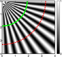
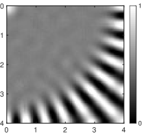
(B)

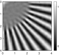
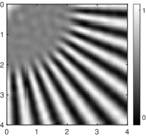
Figure 1: [Row A] Lower-right quarter of the (160$\times$160 pixels) ground-truth fluorescence pattern considered in [1] (left) and deconvolution of the corresponding wide-field image (right). The dashed (resp. solid) lines corresponds to the spatial frequencies transmitted by the OTF support (resp. twice the OTF support). [Row B] Positivity-constrained reconstruction from known illumination patterns: (left) $M=9$ harmonic patterns and (right) $M=200$ speckle patterns. The distance units along the horizontal and vertical axes are given in wavelength $\lambda$.

II-B Super-resolution unveiled

Whereas the mechanism that conveys SR with known structured illuminations is well understood (see [5] for instance), the SR capacity of joint blind-SIM has not been characterized yet. It can be made clear, however, that the positivity constraint (2c) plays a central role in this regard. Let ${\mathb{H}}^{+}$ be the pseudo-inverse of ${\mathb{H}}$ [22, Sec. 5.5.4]. Then, any solution to the problem (2a)-(2b), i.e, without positivity constraints, reads

$$\widehat{{\boldsymbol{\rho}}} =\textbf{Diag}({\mathb{I}}_{0})^{-1}({\mathb{H}}^{+}\overline{{\mathb{y}}}+\overline{{\mathb{q}}}^{\perp})$$ (6a)

$$\widehat{{\mathb{I}}}_{m} =\textbf{Diag}(\widehat{{\boldsymbol{\rho}}})^{-1}({\mathb{H}}^{+}{\mathb{y}}_{m}+{\mathb{q}}_{m}^{\perp}),$$ (6b)

with ${\textstyle\overline{{\mathb{y}}}=\frac{1}{M}\sum_{m}{\mathb{y}}_{m},\quad\text{and}\quad\overline{{\mathb{q}}}^{\perp}=\frac{1}{M}\sum_{m}}{\mathb{q}}_{m}^{\perp}$ where ${\mathb{q}}_{m}^{\perp}$ is an arbitrary element of the kernel of ${\mathb{H}}$, i.e. with arbitrary frequency components above the OTF cutoff frequency. Hence, the formulation (2a)-(2b) has no capacity to discriminate the correct high frequency components, which means that it has no SR capacity. Under the positivity constraint (2c), we thus expect that the SR mechanism rests on the fact that each illumination pattern ${\mathb{I}}_{m}$ activates the positivity constraint on ${\mathb{q}}_{m}$ in a frequent manner.

(A)
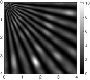
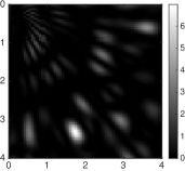
(B)
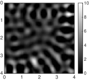
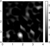
(C)

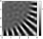
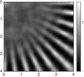
Figure 2: [Row A] One product image ${\mathb{q}}_{m}=\textbf{vect}(\rho_{n}\times I_{m;n})$ built from one of the $200$ illumination patterns used for generating the dataset: (left) a positive constant is added to the standard speckle patterns so that the lowest value is much greater that zero; (right) a positive constant is subtracted to the standard speckle patterns and negative values are set to zero. [Row B] Reconstruction of the product image ${\mathb{q}}_{m}$ that corresponds to the one shown above. [Row C] Final reconstruction $\widehat{{\boldsymbol{\rho}}}$ achieved with the whole set of illuminations —see Subsection II-B for details.

A numerical experiment is now considered to support this assertion. A set of $M$ collected images are simulated following (1) with the PSF ${\mathcal{H}}$ given by the usual Airy pattern that reads in polar coordinates

$${\mathcal{H}}(r,\theta)=\frac{k_{0}^{2}}{\pi}\,\left(\frac{J_{1}(r\,k_{0}\,\text{NA})}{k_{0}\,r}\right)^{2},\qquad r\geq 0,\theta\in{\mathbbm{R}},$$ (7)

where $J_{1}$ is the first order Bessel function of the first kind, NA is the objective numerical aperture set to 1.49, and $k_{0}=2\pi/\lambda$ is the free-space wavenumber with $\lambda$ the emission/excitation wavelength. The ground truth is the 2D ’star-like’ fluorescence pattern depicted in Fig. 1(left). The image sampling step for all the simulations involving the star pattern is set to $\lambda$/20. For this numerical simulation, the illumination set $\{{\mathb{I}}_{m}\}_{m=1}^{M}$ consists in $M=200$ modified speckle patterns, see Fig. 2(A). More precisely, a first set of illuminations is obtained by adding a positive constant (equal to $3$) to each speckle pattern, resulting in illuminations that never activate the positivity constraint in (3). On the contrary, the second set of illuminations is built by subtracting a small positive constant (equal to $0.2$) to each speckle pattern, the negative values being set to zero. The resulting illuminations are thus expected to activate the positivity constraint in (3). For both illumination sets, low-resolution microscope images are simulated and corrupted with Gaussian noise; in this case, the standard deviation was chosen so that the SNR of the total dataset is 40 dB. Corresponding reconstructions of the first product image ${\mathb{q}}_{1}$ obtained via the resolution of (3) is shown in Fig. 2(B), while the retrieved sample (4a) is shown in Fig. 2(C); for each reconstruction, the spatial mean ${\mathb{I}}_{0}$ in (4a) is set to the statistical expectation of the corresponding illumination set. As expected, the reconstruction with the first illumination set is almost identical to the deconvolution of the wide-field image shown in Fig. 1(upper-right), i.e., there is no SR in this case. On the contrary, the second set of illuminations produces a super-resolved reconstruction, hence establishing the central role of the positivity constraint in the original joint reconstruction problem (2).

III A penalized approach for joint Blind-SIM

As underlined in the beginning of Subsection II-B, there is an ambiguity issue concerning the original joint Blind-SIM reconstruction problem. A simple way to enforce unicity is to slightly modify (3) by adding a strictly convex penalization term. We are thus led to solving

$$\min_{{\mathb{q}}_{m}\geq 0}\left\|{\mathb{y}}_{m}-{\mathb{H}}{\mathb{q}}_{m}\right\|^{2}+\varphi({\mathb{q}}_{m}).$$ (8)

Another advantage of such an approach is that $\varphi$ can be chosen so that robustness to the noise is granted and/or some expected features in the solution are enforced. In particular, the analysis conveyed above suggests that favoring sparsity in each ${\mathb{q}}_{m}$ is suited since speckle or periodic illumination patterns tend to frequently cancel or nearly cancel the product images ${\mathb{q}}_{m}$. For such illuminations, the Near-Black Object introduced in Donoho’s seminal paper [12] is an appropriate modeling and, following this line, we found that the separable “$\ell_{1}+\ell_{2}$” penalty provides super-resolved reconstructions:

$$\varphi({\mathb{q}}_{m}):=\alpha{\textstyle\sum_{n}|q_{m;n}|}+\beta||{\mathb{q}}_{m}||^{2},\qquad\alpha\geq 0,\beta>0.$$ (9)

With properly tuned $(\alpha,\beta)$, our joint Blind-SIM strategy is expected to bring SR if “sparse” illumination patterns ${\mathb{I}}_{m}$ are used, i.e., if they enforce $q_{m;n}=0$ for most (or at least many) $n$. More specifically, it is shown in [12, Sec. 4] that SR occurs if the number of non-zero $I_{m;n}$ (i.e., the number of non-zero components to retrieve in ${\mathb{q}}_{m}$) divided by $N$ is lower than $\frac{1}{2}R/N$, with $R/N$ the incompleteness ratio and $R$ the rank of ${\mathb{H}}$. In addition, the resolving power is driven by the spacing between the components to retrieve that, ideally, should be greater than the Rayleigh distance $\frac{\lambda}{2\,\text{NA}}$, see [12, pp. 56-57]. These conditions are rather stringent and hardly met by illumination patterns that can be reasonably considered in practice. These illumination patterns are usually either deterministic harmonic or quasi-harmonic patterns, or random speckle patterns, these latter illuminations being much easier to generate [1]. Nevertheless, in both cases, a SR effect is observed in joint Blind-SIM. Moreover, one can try to maximize this effect via the tuning of some experimental parameters that are left to the designer of the setup. Such parameters are mainly: the period of the light grid and the number of grid shifts for harmonic patterns, the spatial correlation length and the point-wise statistics of the speckle patterns. Investigating the SR properties with respect to these parameters on a theoretical ground seems out of reach. However, a numerical analysis is possible and some illustrative results are now provided that address this question. Reconstructions shown in the sequel are built from (4a) via the numerical resolution of (8)-(9). For sake of clarity, all the algorithmic details concerning this minimization problem are reported in Sec. IV. These simulations were performed with low-resolution microscope images corrupted by additive Gaussian noise such that the signal-to-noise ratio (SNR) of the dataset $\{{\mathb{y}}_{m}\}_{m=1}^{M}$ is 40 dB. In addition, we note that this penalized joint Blind-SIM strategy requires an explicit tuning of some hyper-parameters, namely $\alpha$ and $\beta$ in the regularization function (9). Further details concerning these parameters are reported in Sec. III-D.

(A)
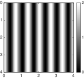
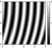
(B)
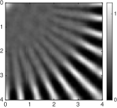
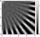
(C)
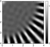
(D)

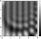
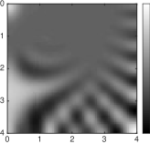
Figure 3: Harmonic patterns: [Row A] One illumination pattern ${\mathb{I}}_{m}$ drawn from the set of regular (left) and distorted (right) harmonic patterns. [Row B] Corresponding penalized joint Blind-SIM reconstructions. [Row C] (left) Decreasing the number of phase shifts from 6 to 3 brings some reconstruction artifacts, see (B-left) for comparison. (right) Increasing the modulation frequency $||{\boldsymbol{\nu}}||$ of the harmonic patterns above the OTF cutoff frequency prevents the super-resolution to occur. [Row D] Low-resolution image ${\mathb{y}}_{m}$ drawn from the dataset for a modulation frequency $||{\boldsymbol{\nu}}||$ lying inside (left) and outside (right) the OTF domain—see Sec. III-A for details.

III-A Regular and distorted harmonic patterns

We first consider unknown harmonic patterns defining a “standard” SIM experiment with $M=18$ patterns. More precisely, the illuminations are harmonic patterns of the form $I({\mathb{r}})=1+\cos(2\pi{\boldsymbol{\nu}}^{t}{\mathb{r}}+\phi)$ where $\phi$ is the phase shift, and with ${\mathb{r}}=(x,y)^{t}$ and ${\boldsymbol{\nu}}=(\nu_{x},\nu_{y})^{t}$ the spatial coordinates and the spatial frequencies of the harmonic function, respectively. Distorted versions of these patterns (deformed by optical aberrations such as astigmatism and coma) were also considered. Three distinct orientations $\theta:=\tan^{-1}(\nu_{y}/\nu_{x})\in\{0,2\pi/3,4\pi/3\}$, for each of which six phase shifts of one sixth of the period, were considered. The frequency of the harmonic patterns $||{\boldsymbol{\nu}}||:=(\nu_{x}^{2}+\nu_{y}^{2})^{1/2}$ is set to 80% of the OTF cutoff frequency, i.e., it lies inside the OTF support.

(A)
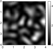
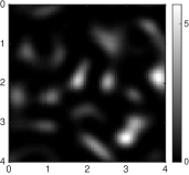
(B)

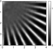
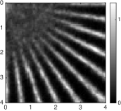
Figure 4: Speckle patterns: [Row A] One speckle illumination such that $\text{NA}_{\text{ill}}=\text{NA}$ (left) and its “squared” counterpart (right). [Row B] Corresponding penalized joint Blind-SIM reconstructions from $M=1000$ speckle (left) and “squared” speckle (right) patterns

One regular and one distorted pattern are depicted in Fig. 3(A) and the penalized joint Blind-SIM reconstructions are shown in Fig. 3(B). For both illumination sets, a clear SR effect occurs, which is similar to the one obtained with the original approach presented in [1]. As expected, however, the reconstruction quality achieved in this blind context is lower than what can be obtained with standard harmonic SIM —for the sake of comparison, see Fig. 1(B). In addition, we note that some artifacts may appear if the number of phase shifts for each orientation is decreased, see Fig. 3(C-left). If we keep in mind that the retrieved sample $\widehat{{\boldsymbol{\rho}}}$ in (4a) gains SR by the summation of (super-resolved) product images $\widehat{{\mathb{q}}}_{m}$, these artifacts are driven (at least partially) by the fact that fewer shifts result in illumination sets that, as a whole, misses to uniformly cancel the plane. In other words, the illumination patterns do cancel the object, but not “that frequently” to bring a uniform SR effect in the final reconstruction. Let us finally investigate how the modulation frequency ${\boldsymbol{\nu}}$ used for the generation of the patterns does impact the SR of the penalized joint Blind-SIM reconstruction. The first finding is that the SR is almost completely lost when $\left\|{\boldsymbol{\nu}}\right\|$ lies beyond the OTF cutoff frequency. As an illustration, the penalized joint Blind-SIM reconstruction shown in Fig. 3(C-right) is obtained with $||{\boldsymbol{\nu}}||$ set to 120% of the OTF cutoff frequency, see also Fig. 1(upper right) for a comparison with deconvolution of the wide-field image. In this case, each harmonic carrier ${\mathb{I}}_{m}$ is completely filtered out from the low-resolution image ${\mathb{y}}_{m}$, see Fig. 3(D). As a result, the SR effect driven by each pattern ${\mathb{I}}_{m}$ is lost since the sparse deconvolution of ${\mathb{y}}_{m}$ (8) does not provide any super-resolved localization of the zeros driven by the illumination patterns.

(A)
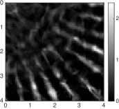
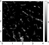
(B)
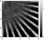
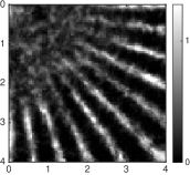
(C)

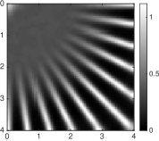
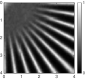
Figure 5: Speckle patterns (continued): Penalized joint Blind-SIM reconstructions from standard speckle (left) and “squared” speckle (right) patterns. The number of illumination patterns considered for reconstruction is $M=10$ (A), $M=200$ (B) and $M=10000$ (C).

III-B Speckle illumination patterns

We now consider second-order stationary speckle illuminations ${\mathb{I}}_{m}$ with known first order statistics $I_{0;n}=I_{0},\forall n$. Each one of these patterns is a fully-developed speckle drawn from the point-wise intensity of a correlated circular Gaussian random field. The correlation is adjusted so that the pattern ${\mathb{I}}_{m}$ exhibits a spatial correlation of the form (7) but with “numerical aperture” parameter NA${}_{\text{ill}}$ that sets the correlation length to $\frac{\lambda}{2\,\text{NA}_{\text{ill}}}$ within the random field. As an illustration, the speckle pattern shown in Fig. 4(A-left) was generated in the standard case $\text{NA}_{\text{ill}}=\text{NA}$. From this set of regular (fully-developed) speckle patterns, we also consider another set of random illumination patterns built by squaring each speckle pattern, see Fig. 4(A). These “squared” patterns are considered hereafter because they give a deeper insight about the SR mechanism at work in joint Blind-SIM. Moreover, we discuss later in this subsection that these patterns can be generated with other microscopy techniques, hence extending the concept of random illumination microscope to other optical configurations. From a statistical viewpoint, the probability distribution function (pdf) of “standard” and “squared” speckle patterns differ. For instance, the pdf of the squared speckle intensity is more concentrated around zero than the exponential pdf of the standard speckle intensity. In addition, the spatial correlation is also changed since the power spectral density of the “squared” random field spans twice the initial support of its speckle counterpart [23]. As a result, the “squared” speckle grains are sharper, and they enjoy larger spatial separation. According to previous SR theoretical results [12, p. 57] (see also the beginning of Sec. III), these features may bring more SR in joint Blind-SIM than standard speckle patterns. This assumption was indeed corroborated by our simulations. For instance, the reconstructions in Fig. 4(B) were obtained from a single set of $M=1000$ speckle patterns such that $\text{NA}_{\text{ill}}=\text{NA}$: in this case, the “squared” illuminations (obtained by squaring the speckle patterns) provide a higher level of SR than the standard speckle illuminations. Figure 5 shows how the reconstruction quality varies with the number of illumination patterns. With very few illuminations, the sample is retrieved in the few places that are activated by the “hot spots” of the speckle patterns. This actually illustrates that the joint Blind-SIM approach is also an “activation” strategy in the spirit of PALM [13] and STORM [14]. With our strategy, the activation process is nevertheless enforced by the structured illumination patterns and not by the fluorescent markers staining the sample. This effect is more visible with the squared illumination patterns and, with these somehow sparser illuminations, the number of patterns needs to be increased so that the fluctuations in $\sum_{m}{\mathb{I}}_{m}$ is moderate, hence making the equality (2b) a legitimate constraint. We also stress that these simulations corroborate the empirical statement that $M\approx 9$ harmonic illuminations and $M\approx 200$ speckle illuminations produce comparable super-resolved reconstructions, see Fig. 3(C-left) and Fig. 5(B-left). Obviously, imaging with random speckle patterns remains an attractive strategy since it is achieved with a very simple experimental setup, see [1] for details.

(A)
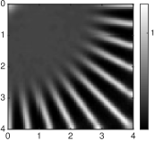
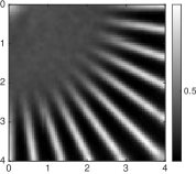
(B)
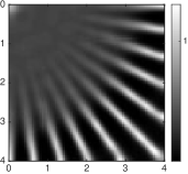
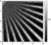
(C)

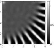
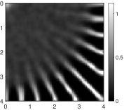
Figure 6: Speckle patterns (continued): The correlation length of speckle and “squared” speckle patterns drives the level of super-resolution in the penalized joint Blind-SIM reconstruction: [Rows A] reconstruction from $M=10000$ speckle patterns with $\text{NA}_{\text{ill}}=0.5\,\text{NA}$ (left) and from the corresponding “squared” random-patterns (right). [Rows B] idem with $\text{NA}_{\text{ill}}=2\,\text{NA}$. [Rows C] idem with uncorrelated patterns.

For both random patterns, we also note that increasing the correlation length above the Rayleigh distance $\frac{\lambda}{2\,\text{NA}}$ (i.e., setting $\text{NA}_{\text{ill}}<\text{NA}$) deteriorates the SR whereas, conversely, taking $\text{NA}_{\text{ill}}=2\text{NA}$ enhances it, see Fig. 6-(A,B). However, the resolving power of the joint Blind-SIM estimate deteriorates if the correlation length is further decreased; for instance, uncorrelated speckle patterns are finally found to hardly produce any SR, see Fig. 6-(C). Indeed, with arbitrary small correlation lengths, many “hot spots” tend to be generated within a single Rayleigh distance, leading to this loss in the resolving power. Obviously, the “squared” speckle patterns are less sensitive to this problem because they are inherently sparser.

Finally, the experimental relevance of the simulations involving “squared” speckle illuminations needs to be addressed. Since a two-photon (2P) fluorescence interaction is sensitive to the square of the intensity [24], most of these simulations can actually be considered as wide-field 2P structured illumination experiments. Unlike one-photon (i.e., fully-developed) speckle illuminations, though, a 2P interaction requires an excitation wavelength $\lambda_{\text{ill}}\sim 1000$ nm that is roughly twice the one of the collected fluorescence $\lambda_{\text{det}}\sim 500$ nm. The lateral 2P correlation length being $\frac{\lambda_{\text{ill}}}{4\text{NA}_{\text{ill}}}$, epi-illumination setups with one-photon (1P) and 2P illuminations provide similar lateral correlation lengths. This 2P instrumental configuration is simulated in Fig. 6(A-right), which does not show any significant SR improvement with respect to 1P epi-illumination interaction shown in Fig. 5(C-left). The increased SR effect driven by “squared” illumination patterns can nevertheless be obtained with 2P interactions if the excitation and the collection are performed with separate objectives. For instance, the behaviors shown in Fig. 5(C-right) and in Fig. 6(B-right) can be obtained if the excitation NA is, respectively, twice and four times the collection NA. With these configurations, the 2P excitation exhibits a correlation length which is significantly smaller than the one driven by the objective PSF, and a strong SR improvement is observed in simulation by joint Blind-SIM. The less spectacular simulation shown in Fig. 6(C-right) can also be considered as a 2P excitation, in the “limit” case of a very low collection NA. The 1P simulation shown in Fig. 6(C-left) rather mock a photo-acoustic imaging experiment[19], an imaging technique for which the illumination lateral correlation length is negligible with respect to the PSF width.

As a final remark, we stress that 2P interactions are not the only way to generate sparse illumination patterns for the joint Blind-SIM. In particular, super-Rayleigh speckle patterns [26] are promising candidates for that purpose.

(A)
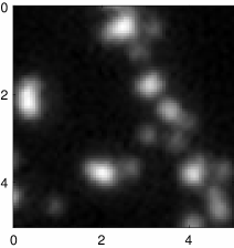
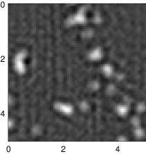
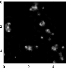
(B)

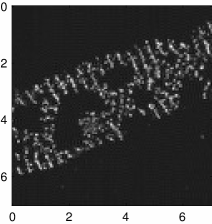
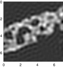
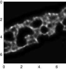
Figure 7: Processing of real and mock data: [Row A] Fluorescent beads with diameters of 100 nm are illuminated by 100 fully-developed (i.e., one-photon) speckle patterns through an illumination/collection objective ($\text{NA}=1.49$). The sum of the acquisitions of the fluorescent light (left) and its Wiener deconvolution (middle) provide diffraction limited images of the beads. The joint Blind-SIM reconstruction performed with the hyper-parameters set to $\beta=5\times 10^{-5}$ and $\alpha=0.4$ is significantly more resolved (right). The sampling rate used in these images is 32.5 nm, corresponding to an up-sampling factor of two with respect to the camera sampling. [Row B] STORM reconstruction of a marked rat neuron showing a lattice structure with a 190-nm periodicity (left). Deconvolution of the simulated wide-field image (middle). Joint Blind-SIM reconstruction of the sample obtained from 300 (one-photon) speckle patterns; the hyper-parameters are set to $\beta=2\times 10^{-5}$ and $\alpha=1.5$ (right). The sampling rate of the STORM ground-truth image is 11.4 nm. The sampling rate of the joint Blind-SIM reconstruction is 28.5 nm, corresponding to an up-sampling factor of four with respect to the camera sampling. The distance units along the horizontal and vertical axes are given in wavelength $\lambda_{\text{coll}}$, i.e., 520 nm in row A and 488 nm in row B.

III-C Some reconstructions from real and mock data

The star test-pattern used so far is a simple and legitimate mean to evaluate the resolving power of our strategy [27], but it hardly provides a convincing illustration of what can be expected with real data. Therefore, we now consider the processing of more realistic datasets with joint Blind-SIM. In this section, the microscope acquisitions are all designed so that the spatial sampling rate is equal or slightly above the Nyquist rate $\frac{\lambda}{4\text{NA}}$. As a consequence, a preliminary up-sampling step of the camera acquisitions is performed so that their sampling rate reaches that of the super-resolved reconstruction.

As a first illustration, we consider a real dataset resulting from a test sample composed of fluorescent beads with diameters of 100 nm. A set of $100$ one-photon speckle patterns is generated by a spatial light modulator and a laser source operating at $\lambda_{\text{ill}}=488$ nm. The fluorescent light at $\lambda_{\text{coll}}=520$ nm is collected through an objective with $\text{NA}=1.49$ and recorded by a camera. The excitation and the collection of the emitted light are performed through the same objective, i.e., the setup is in epi-illumination mode. The total number of photons per camera pixels is about $65\,000$. In the perspective of further processing, this set of camera acquisitions is first up-sampled with a factor of two. Figure 7(A-left) shows the sum of these (up-sampled) acquisitions, which is similar to a wide-field image. Wiener deconvolution of this image can be performed so that all spatial frequencies transmitted by the OTF are equivalently contributing in a diffraction-limited image of the beads, see Figure 7(A-middle). The processing of the dataset by the joint Blind-SIM strategy shown in Figure 7(A-right) reveals several beads that are otherwise unresolved on the diffraction-limited images, hence demonstrating a clear SR effect. In this case, the distance between the closest pair of resolved beads provides an upper bound for the final resolution, that is $\lambda_{\text{coll}}/5$.

The experimental demonstration above does not involve any biological sample, and we now consider a simulation designed to be close to a “real-world” biological experiment. More specifically, the STORM reconstruction of a marked neuron is used as a ground truth to simulate a series of microscope acquisitions generated from one-photon speckle illuminations. Our simulation considers 300 illuminations and acquisitions, both performed through the same objective, at $\lambda=488$ nm and with NA $=1$. Each low-resolution acquisition is finally plagued with Poisson noise, the total photon budget being equal to $50\,000$ so that it fits to the one of a standard fluorescence wide-field image. The sample (ground truth) shown in Figure 7(B-left) interestingly exhibits a lattice structure with a 190 nm periodicity (in average) that is not resolved by the diffracted-limited image shown in Figure 7(B-middle). The joint Blind-SIM reconstruction in Figure 7(A-right) shows a significant improvement of the resolution, which reveals some parts of the underlying structure.

III-D Tuning the regularization parameters

The tuning of parameters $\alpha$ and $\beta$ in (9) is a pivotal issue since inappropriate values result in deteriorated reconstructions. On the one hand, the quadratic penalty in (9) was mostly introduced to ensure that the minimizer defined by (8) is unique (via strict convexity of the criterion). However, because high-frequency components in $\widehat{{\mathb{q}}}_{m}$ are progressively damped as $\beta$ increases, the latter parameter can also be adjusted in order to prevent an over-amplification of the instrumental noise. A trade-off should nevertheless be sought since large values of $\beta$ prevent super-resolution to occur. For a given SNR, $\beta$ is then maintained to a fixed (usually small) value. For instance, we chose $\beta=10^{-6}$ for all the simulations involving the star pattern in this paper since they were performed with a rather favorable SNR. On the other hand, the quality of reconstruction crucially depends on parameter $\alpha$. More precisely, larger values of $\alpha$ will provide sparser solutions $\widehat{{\mathb{q}}}_{m}$, and thus a sparser reconstructed object $\widehat{{\boldsymbol{\rho}}}$. Fig. 8 shows an example of under-regularized and over-regularized solutions, respectively corresponding to a too small and a too large value of $\alpha$. The prediction of the appropriate level of sparsity to seek for each ${\mathb{q}}_{m}$, or equivalently the tuning of the regularization parameter $\alpha$, is not an easy task. Two main approaches can be considered. One relies on automatic tuning. For instance, a simple method called Morozov’s discrepancy principle considers that the least-squares terms $\left\|{\mathb{y}}_{m}-{\mathb{H}}\widehat{{\mathb{q}}}_{m}\right\|^{2}$ should be chosen in proportion with the variance of the additive noise, the latter being assumed known [29]. Other possibilities seek a trade-off between $\left\|{\mathb{y}}_{m}-{\mathb{H}}\widehat{{\mathb{q}}}_{m}\right\|^{2}$ and $\varphi(\widehat{{\mathb{q}}}_{m})$. This is the case with the L-curve [30], but also with the recent contribution [31], which deals with a situation comparable to ours. Another option relies on a Bayesian interpretation of $\widehat{{\mathb{q}}}_{m}$ as a maximum a posteriori solution, which opens the way to the estimation of $\alpha$ marginally of ${\mathb{q}}_{m}$. In this setting, Markov Chain Monte Carlo sampling [32] or variational Bayes methods [33] could be employed. An alternate approach to automatic tuning consists in relying on a calibration step. It amounts to consider that similar acquisition conditions, applied to a given type of biological samples, lead to similar ranges of admissible values for the tuning of $\alpha$. The validation of such a principle is however outside the scope of this article as it requires various experimental acquisitions from biological samples with known structures (or, at least, with some calibrated test patterns). Concerning the examples proposed in the present section, the much simpler strategy consisted in selecting the reconstruction which is visually the “best” among the reconstructed images with varying $\alpha$.

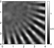
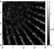
Figure 8: Penalized Blind-SIM reconstructions from the dataset used to generate the super-resolved reconstruction shown in Fig. 4(B-left). The hyper-parameter $\beta$ was set to $10^{-6}$ in any case, and $\alpha$ was set to $10^{-3}$ (left) and $0.9$ (right). For the sake of comparison, our tuning for the reconstruction shown in Fig. 4(B-left) is $\beta=10^{-6}$ and $\alpha=0.3$.

IV A new preconditioned proximal iteration

We now consider the algorithmic issues involved in the constrained optimization problem (8)-(9). For sake of simplicity, the subscript $m$ in ${\mathb{y}}_{m}$ and ${\mathb{q}}_{m}$ will be dropped. The reader should however keep in mind that the algorithms presented below only aim at solving one of the $M$ sub-problems involved in the final joint Blind-SIM reconstruction. Moreover, we stress that all simulations presented in this article are performed with a convolution matrix ${\mathb{H}}$ with a block-circulant with circulant-block (BCCB) structure. The more general case of block-Toeplitz with Toeplitz-block (BTTB) structure is shortly addressed at the end of Subsection IV-C.

At first, let us note that (8)-(9) is an instance of the more general problem

$$\min_{{\mathb{q}}\in{\mathbbm{R}}^{N}}\left[f({\mathb{q}}):=g({\mathb{q}})+h({\mathb{q}})\right]$$ (10)

where $g$ and $h$ are closed-convex functions that may not share the same regularity assumptions: $g$ is supposed to be a smooth function with a $L$-Lipschitz continuous gradient $\boldsymbol{\nabla}g$, but $h$ does not need to be smooth. Such a splitting aims at solving constrained non-smooth optimization problems by proximal (or forward-backward) iterations. The next subsection presents the basic proximal algorithm and the well-known FISTA that usually improves the convergence speed.

IV-A Basic proximal and FISTA iterations

We first present the resolution of (10) in a general setting, then the penalized joint Blind-SIM problem (8) is addressed as our particular case of interest.

IV-A1 General setting

Let ${\mathb{q}}^{(0)}$ be an arbitrary initial guess, the basic proximal update $k\rightarrow k+1$ for minimizing the convex criterion $f$ is [34, 35, 36]

$${\mathb{q}}^{(k+1)}~{}\longleftarrow~{}{\mathcal{P}}_{\gamma h}\left({\mathb{q}}^{(k)}-\gamma\boldsymbol{\nabla}g({\mathb{q}}^{(k)})\right)$$ (11)

where ${\mathcal{P}}_{\gamma h}$ is the proximity operator (or Moreau envelope) of the function $\gamma h$ [37, p.339]

$${\mathcal{P}}_{\gamma h}({\mathb{q}}):=\mathop{\mathrm{arg\,min}}_{{\mathb{x}}\in{\mathbbm{R}}^{N}}\left[h({\mathb{x}})+\frac{1}{2\gamma}||{\mathb{x}}-{\mathb{q}}||^{2}\right].$$ (12)

Although this operator defines the update implicitly, an explicit form is actually available for many of the functions met in signal and image processing applications, see for instance [36, Table 10.2]. The Lipschitz constant $L$ granted to $\boldsymbol{\nabla}g$ plays an important role in the convergence of iterations (11). In particular, global convergence toward a solution of (10) occurs as long as the step size $\gamma$ is chosen such that $0<\gamma<2/L$. However, the convergence speed is usually very low and the following accelerated version named FISTA [38] is usually preferred

$${\mathb{q}}^{(k+1)}~{}\longleftarrow~{}{\mathcal{P}}_{\gamma h}\left({\boldsymbol{\omega}}^{(k)}-\gamma\boldsymbol{\nabla}g({\boldsymbol{\omega}}^{(k)})\right)$$ (13a)

$${\boldsymbol{\omega}}^{(k+1)}~{}\longleftarrow~{}{\mathb{q}}^{(k+1)}+{\textstyle\frac{k-1}{k+2}}\big{(}{\mathb{q}}^{(k+1)}-{\mathb{q}}^{(k)}\big{)}.$$ (13b)

The convergence speed toward $\min_{\mathb{q}}f({\mathb{q}})$ achieved by (13) is $O(1/k^{2})$, which is often considered as a substantial gain compared to the $O(1/k)$ rate of the basic proximal iteration. It should be noted however that this “accelerated” form may not always provide a faster convergence speed with respect to its standard counterpart, see for instance [36, Fig. 10.2]. FISTA was nevertheless found to be faster for solving the constrained minimization problem involved in joint Blind-SIM, see Fig. 11. We finally stress that convergence of (13) is granted for $0<\gamma<1/L$ [38].

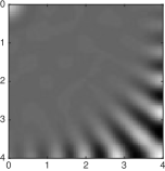
(a) FISTA 10 it.		(d) PPDS 10 it.
(b) FISTA 50 it.		(e) PPDS 50 it.
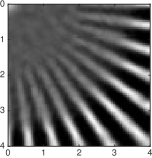
(c) FISTA 1000 it.		(f) PPDS 1000 it.

Figure 9: Harmonic joint Blind-SIM reconstruction of the fluorescence pattern achieved by the minimization of the criterion (8) with 10, 50 or 1000 FISTA (abc) or PPDS (def) iterations. For all these simulations, the initial-guess is ${\mathb{q}}^{(0)}=\textbf{0}$ and the regularization parameters is set to $(\alpha=0.3,\beta=10^{-6})$. The PPDS iteration implements the preconditioner given in (28) with ${\mathb{C}}={\mathb{H}}^{t}{\mathb{H}}$ and $a=1$, see Sec IV-C for details.

IV-A2 Solution of the $m$-th joint Blind-SIM sub-problem

For the penalized joint Blind-SIM problem considered in this paper, the minimization problem (8) [equipped with the penalty (9)] takes the form (10) with

$$g({\mathb{q}}) \,=\,||{\mathb{y}}-{\mathb{H}}{\mathb{q}}||^{2}+\beta||{\mathb{q}}||^{2}$$ (14a)

$$h({\mathb{q}}) \,=\,\alpha\sum_{n}\phi(q_{n})$$ (14b)

where $$\phi:{\mathbbm{R}}\rightarrow{\mathbbm{R}}\cup\{+\infty\}$$ is such that

$$\phi(u) :=\left\{\begin{tabular}[]{@{\kern 1pt}ll}.0pt\lx@intercol$u$&\quad if $u\geq 0$.\\[-1.99997pt] .0pt\lx@intercol$+\infty$&\quad otherwise.\end{tabular}\right.$$ (14e)

The gradient of the regular part in the splitting

$$\boldsymbol{\nabla}g({\mathb{q}})=2\left[{\mathb{H}}^{t}({\mathb{H}}{\mathb{q}}-{\mathb{y}})+\beta{\mathb{q}}\right]$$ (15)

is $L$-Lipschitz-continuous with $L=2\left(\lambda_{\text{max}}({\mathb{H}}^{t}{\mathb{H}})+\beta\right)$ where $\lambda_{\text{max}}({\mathb{A}})$ denotes the highest eigenvalue of the matrix ${\mathb{A}}$. Furthermore, the proximity operator (12) with $h$ defined by (14b) leads to the well-known soft-thresholding rule [39, 40]

$${\mathcal{P}}_{\gamma h}({\mathb{q}})=\textbf{vect}\left(\max\{q_{n}-\gamma\alpha,0\}\right).$$ (16)

From a practical perspective, both the basic iteration (11) and its accelerated counterpart (13) are easily implemented at a very low computational cost from equations (15) and (16). For our penalized joint Blind-SIM approach, however, we observed that both algorithms exhibit similar convergence behavior in terms of visual aspect of the current estimate. The convergence speed is also significantly slow: several hundreds of iterations are usually required for solving the $M=200$ sub-problems involved in the joint Blind-SIM reconstruction shown in Fig. 5(B). In addition, Fig. 9(a-c) shows the reconstruction built with ten, fifty and one thousand FISTA iterations. Clearly, we would like that this latter quality of reconstruction is reached in a reasonable amount of time. The next subsection introduces a preconditioned primal-dual splitting strategy that achieves a much higher convergence speed, as illustrated by Fig. 9(right).

IV-B Preconditioned primal-dual splitting

The preconditioning technique [42, p. 69] is formally equivalent to addressing the initial minimization problem (10) via a linear transformation ${\mathb{q}}:={\mathb{P}}{\mathb{v}}$, where ${\mathb{P}}\in{\mathbbm{R}}^{N\times N}$ is a symmetric positive-definite matrix. There is no formal difficulty in defining a preconditioned version of the proximal iteration (11). However, if one excepts the special case of diagonal matrices ${\mathb{P}}$ [43, 44, 45, 46], the proximity operator of ${\mathcal{H}}({\mathb{v}}):=h({\mathb{P}}{\mathb{v}})$ cannot be obtained explicitly and needs to be computed approximately. As a result, solving a nested optimization problem is required at each iteration, hence increasing the overall computational cost of the algorithm and raising a convergence issue since the sub-iterations must be truncated in practice [45, 47]. Despite this difficulty, the preconditioning is widely accepted as a very effective way for accelerating proximal iterations. In the sequel, the versatile primal-dual splitting technique introduced in [11, 48, 49] is used to propose a new preconditioned proximal iteration, without any nested optimization problem.

This new preconditioning technique is now presented for the generic problem (10). At first, we express the criterion $f$ with respect to the transformed variables

$$f({\mathb{P}}{\mathb{v}}) ={\mathcal{G}}({\mathb{v}})+h({\mathb{P}}{\mathb{v}})$$ (17)

with ${\mathcal{G}}({\mathb{v}}):=g({\mathb{P}}{\mathb{v}})$. Since the criterion above is a particular case of the form considered in [11, Eq. (45)], it can be optimized by a primal-dual iteration [11, Eq. (55)] that reads

$${\mathb{v}}^{(k+1)} \longleftarrow{\mathb{v}}^{(k)}-\theta\tau{\mathb{d}}^{(k)}$$ (18a)

$${\boldsymbol{\omega}}^{(k+1)} \longleftarrow{\boldsymbol{\omega}}^{(k)}+\theta{\boldsymbol{\Delta}}^{(k)}$$ (18b)

with

$${\mathb{d}}^{(k)} :=\boldsymbol{\nabla}{\mathcal{G}}({\mathb{v}}^{(k)})+{\mathb{P}}{\boldsymbol{\omega}}^{(k)}$$ (19a)

$${\boldsymbol{\Delta}}^{(k)} :={\mathcal{P}}_{\sigma h^{\star}}\big{(}{\boldsymbol{\omega}}^{(k)}+\sigma{\mathb{P}}({\mathb{v}}^{(k)}-2\tau{\mathb{d}}^{(k)})\big{)}-{\boldsymbol{\omega}}^{(k)}$$ (19b)

where the proximal mapping applied to $h^{\star}$, the Fenchel conjugate function for $h$, is easily obtained from

$${\mathcal{P}}_{\sigma h^{\star}}({\boldsymbol{\omega}})={\boldsymbol{\omega}}-\sigma{\mathcal{P}}_{h/\sigma}({\boldsymbol{\omega}}/\sigma).$$ (20)

The primal update (18a) can also be expressed with respect to the untransformed variables ${\mathb{q}}$:

$${\mathb{q}}^{(k+1)} \longleftarrow{\mathb{q}}^{(k)}-\theta\tau{\mathb{B}}{\boldsymbol{\zeta}}^{(k)}$$ (21)

with ${\boldsymbol{\zeta}}^{(k)}:=\boldsymbol{\nabla}g({\mathb{q}}^{(k)})+{\boldsymbol{\omega}}^{(k)}$ and ${\mathb{B}}:={\mathb{P}}{\mathb{P}}$. Since the update (21) is a preconditioned primal step, we expect that a clever choice of the preconditioning matrix ${\mathb{B}}$ will provide a significant acceleration of the primal-dual  procedure. In addition, we note that the quantity ${\mathb{a}}^{(k)}:={\boldsymbol{\omega}}^{(k)}+\sigma{\mathb{P}}({\mathb{v}}^{(k)}-2\tau{\mathb{d}}^{(k)})$ involved in the dual step via (19b) also reads

$${\mathb{a}}^{(k)} :={\boldsymbol{\omega}}^{(k)}+\sigma({\mathb{q}}^{(k)}-2\tau{\mathb{B}}{\boldsymbol{\zeta}}^{(k)}).$$ (22)

Hereafter, the primal-dual updating pair (18b) and (21) is called a preconditioned primal-dual splitting (PPDS) iteration. Following [11, Theorem 5.1], the convergence of these PPDS iterations is granted if the following conditions are met for the parameters $(\theta,\tau,\sigma)$:

$$\sigma>0,~{}\tau>0,~{}\theta >0$$ (23a)

$$\gamma_{\tau,\sigma} \in[1;2)$$ (23b)

$$\gamma_{\tau,\sigma} >\theta$$ (23c)

with $\gamma_{\tau,\sigma}:=2-\tau\left[1-\tau\sigma\lambda_{\text{max}}({\mathb{B}})\right]^{-1}{\mathcal{L}}/2$, where ${\mathcal{L}}$ is the Lipschitz-continuity constant of $\boldsymbol{\nabla}{\mathcal{G}}$, see Eq. (17). Within the convergence domain ensured by (23), the practical tuning of the parameter set $(\theta,\tau,\sigma)$ is tedious as it may impair the convergence speed. We propose the following tuning strategy, which appeared to be very efficient. At first, we note that the step length $\tau$ relates only to the primal update (18a) whereas $\sigma$ relates only to the dual update (18b) via ${\boldsymbol{\Delta}}^{(k)}$. In addition, the relaxation parameter $\theta$ scales both the primal and the dual steps (18). Considering only under-relaxation (i.e., $\theta<1$), (23c) is unnecessary and (23b) is equivalent to the following bound

$$\sigma\leq\overline{\sigma}\quad\text{with}\quad\overline{\sigma}:=\big{(}1/\tau-{\mathcal{L}}/2\big{)}\,\lambda^{-1}_{\text{max}}({\mathb{B}}).$$ (24)

This relation defines an admissible domain for $(\tau,\sigma)$ under the condition $\theta<1$, see Fig. 10.

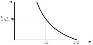
Figure 10: Admissible domain for $(\tau,\sigma)$ ensuring the global convergence of the PPDS iteration with $\theta\in(0;1)$, see Equation (24).

Our strategy defines $\tau$ as the single tuning parameter of our PPDS iteration, the parameter $\sigma$ being adjusted so that the dual step is maximized:

$$0<\tau<\overline{\tau},\quad\sigma=\overline{\sigma}\quad\text{and}\quad\theta=0.99,$$ (25)

with $\overline{\tau}:=2/{\mathcal{L}}$. We set $\theta$ arbitrary close to 1 since practical evidence indicates that under-relaxing $\theta$ slows down the convergence rate. The numerical evaluation of the bounds $\overline{\tau}$ and $\overline{\sigma}$ is application-dependent since they depend on ${\mathcal{L}}$ and $\lambda_{\text{max}}({\mathb{B}})$.

IV-C Resolution of the joint Blind-SIM sub-problem

For our specific problem, the implementation of the PPDS iteration requires first the conjugate function (20): with $h$ defined by (14b), the Fenchel conjugate is easily found and reads

$${\mathcal{P}}_{\sigma h^{\star}}({\boldsymbol{\omega}})=\textbf{vect}\left(\text{min}\left\{\omega_{n},\alpha\right\}\right).$$ (26)

The updating rule for the PPDS iteration then reads

$${\mathb{q}}^{(k+1)}\longleftarrow{\mathb{q}}^{(k)}-\theta\tau{\mathb{B}}{\boldsymbol{\zeta}}^{(k)}$$ (27a)

$${\boldsymbol{\omega}}^{(k+1)}\longleftarrow{\boldsymbol{\omega}}^{(k)}+\theta{\boldsymbol{\Delta}}^{(k)}$$ (27b)

with ${\boldsymbol{\Delta}}^{(k)}=\textbf{vect}\big{(}\text{min}\{a_{n}^{(k)},\alpha\}\big{)}-{\boldsymbol{\omega}}^{(k)}$ and $a_{n}^{(k)}$ the $n$th component of the vector ${\mathb{a}}^{(k)}$ defined in (22). We note that the positivity constraint is not enforced in the primal update (27a). Primal feasibility (i.e. positivity) therefore occurs only asymptotically thanks to the global convergence of the sequence (27) toward the minimizer of the functional (14). Compared to FISTA, this behavior may be considered as a drawback of the PPDS iteration. However, we do believe that the ability of the PPDS iteration to “transfer” the hard constraint from the primal to the dual step is precisely the cornerstone of the acceleration provided by preconditioning. Obviously, such an acceleration requires that the preconditioner ${\mathb{B}}$ is wisely chosen. For our joint Blind-SIM problem, the preconditioning matrix is derived from Geman and Yang semi-quadratic construction [50], [51, Eq. (6)]

$${\mathb{B}}=\frac{1}{2}\left({\mathb{C}}+\beta\,{\mathb{I}}_{d}/a\right)^{-1}$$ (28)

where ${\mathb{I}}_{d}$ is the identity matrix and $a>0$ is a free parameter of the preconditioner. We choose ${\mathb{C}}$ in the class of positive semi-definite matrix with a BCCB structure [41, Sec. 5.2.5]. This choice enforces that ${\mathb{B}}$ is also BCCB, which considerably helps in reducing the computational burden: ($i$) ${\mathb{B}}$ can be stored efficiently and ($ii$) the matrix-vector product ${\mathb{B}}{\boldsymbol{\zeta}}^{(k)}$ in (27a) can be computed with ${\mathcal{O}}(N\log N)$ complexity by the bidimensional fast Fourier transform (FFT) algorithm. Obviously, if the observation model ${\mathb{H}}$ is also a BCCB matrix built from the discretized OTF, the choice ${\mathb{C}}={\mathb{H}}^{t}{\mathb{H}}$ in (28) leads to ${\mathb{B}}=(\boldsymbol{\nabla}^{2}g)^{-1}$ for $a=1$. Such a preconditioner is expected to bring the fastest asymptotic convergence since it corrects the curvature anisotropies induced by the regular part $g$ in the criterion (10).

The PPDS pseudo-code for solving the joint Blind-SIM problem is given in Algorithm 1.

1   Given quantities:

2PSF ${\mathb{h}}$, Dataset $\{{\mathb{y}}_{m}\}_{m=1}^{M}$, Average intensity ${\mathb{I}}_{0}\in{\mathbbm{R}}^{N}_{+}$;

3 Regularization parameters: $\beta,\alpha\in{\mathbbm{R}}_{+}$;

4PPDS parameters: $a\in{\mathbbm{R}}_{+}$; $\theta\in(0,1)$; $\tau\in(0,2{\mathcal{L}})$; $k_{\text{max}}\in{\mathbbm{N}}$;

5 Initial guesses: $\{{\mathb{q}}_{m}^{(0)},{\boldsymbol{\omega}}_{m}^{(0)}\}_{m=1}^{M}$;

6[.5em]   $\widehat{{\boldsymbol{\rho}}}\longleftarrow\textbf{0}$; $\sigma\longleftarrow\overline{\sigma}$ [see (24)];

7 $\widetilde{{\mathb{h}}}\longleftarrow\text{FFT}({\mathb{h}})$; $\widetilde{{\boldsymbol{\gamma}}}\longleftarrow\widetilde{{\mathb{h}}}^{*}\odot\widetilde{{\mathb{h}}}$; $\widetilde{{\mathb{b}}}\longleftarrow(2\widetilde{{\boldsymbol{\gamma}}}+2\beta/a)$;

8 // The outer loop: processing each view ${\mathb{y}}_{m}$…

9for $m=1\cdots M$ do

10       $\widetilde{{\mathb{y}}}\longleftarrow\text{FFT}({\mathb{y}}_{m})$; $\widetilde{{\mathb{q}}}^{(0)}\longleftarrow\text{FFT}({\mathb{q}}_{m}^{(0)})$; $\widetilde{{\boldsymbol{\omega}}}^{(0)}\longleftarrow\text{FFT}({\boldsymbol{\omega}}_{m}^{(0)})$;

11       // The inner loop: PPDS minimization…

12       for $k=0\cdots k_{\text{max}}$  do

13            

14             // The primal step (Fourier domain)…

15             $\widetilde{{\mathb{d}}}^{(k)}\longleftarrow\left(\widetilde{{\boldsymbol{\omega}}}^{(k)}-2(\widetilde{{\mathb{h}}}\odot\widetilde{{\mathb{y}}}-(\widetilde{{\boldsymbol{\gamma}}}+\beta)\odot\widetilde{{\mathb{q}}}^{(k)})\right)\oslash\widetilde{{\mathb{b}}}$;

16             $\widetilde{{\mathb{q}}}^{(k+1)}\longleftarrow\widetilde{{\mathb{q}}}^{(k)}-\theta\tau\widetilde{{\mathb{d}}}^{(k)}$;

17             // The dual step (direct domain)…

18             ${\mathb{a}}^{(k)}\longleftarrow\text{FFT}^{-1}\left(\widetilde{{\boldsymbol{\omega}}}^{(k)}+\sigma(\widetilde{{\mathb{q}}}^{(k)}-2\tau\widetilde{{\mathb{d}}}^{(k)})\right)$;

19             ${\boldsymbol{\omega}}^{(k+1)}\longleftarrow(1-\theta)\,{\boldsymbol{\omega}}^{(k)}+\theta\,\textbf{vect}(\text{min}\{a_{n}^{(k)},\alpha\})$;

20             // Prepare next PPDS iteration…

21             $\widetilde{{\mathb{q}}}^{(k)}\longleftarrow\widetilde{{\mathb{q}}}^{(k+1)}$; $\widetilde{{\boldsymbol{\omega}}}^{(k)}\longleftarrow\text{FFT}({\boldsymbol{\omega}}^{(k+1)})$;

22            

23       end for

24       // Building-up the joint Blind-SIM estimate…

25      $\widehat{{\boldsymbol{\rho}}}\longleftarrow\widehat{{\boldsymbol{\rho}}}+\frac{1}{M}\text{FFT}^{-1}(\widetilde{{\mathb{q}}}^{(k)})\oslash{\mathb{I}}_{0}$;

26      

27 end for

28   Final result: The joint Blind-SIM estimate is stored in $\widehat{{\boldsymbol{\rho}}}$

[.5em]  

Algorithm 1 Pseudo-Code of the joint Blind-SIM PPDS algorithm, assuming that ${\mathb{H}}$ is a BCCB matrix and ${\mathb{C}}={\mathb{H}}^{t}{\mathb{H}}$. The symbols $\odot$ and $\oslash$ are the component-wise product and division, respectively. For the sake of simplicity, this pseudo-code implements a very simple stopping rule based on a maximum number of minimizing steps, see line 1. In practice, a more elaborated stopping rule could be used by monitoring the norm $||{\boldsymbol{\zeta}}^{(k)}||$ defined by (21) since it tends towards 0 as ${\mathb{q}}^{(k)}$ asymptotically reaches the constrained minimizer of the $m$-th nested problem.

This pseudo-code requires that ${\mathcal{L}}$ and $\lambda_{\text{max}}({\mathb{B}})$ are given for the tuning (25): we get

$$\lambda_{\text{max}}({\mathb{B}})\,=\,1/\lambda_{\text{min}}({\mathb{B}}^{-1})\,=\,a\,(2\beta)^{-1}$$ (29a)

since $${\mathb{H}} {\mathcal{L}}=\lambda_{\text{max}}({\mathb{B}}\,\boldsymbol{\nabla}^{2}g)$$ is rank deficient in our context, and the Lipschitz constant that reads can be further simplified as

$${\mathcal{L}}=\left\{\begin{array}[]{ll}a&\text{if $a\geq 1$}\\ {\displaystyle(\widetilde{\gamma}_{\text{max}}+\beta)(\widetilde{\gamma}_{\text{max}}+\beta/a)^{-1}}&\text{otherwise},\end{array}\right.$$ (29d)

with $\widetilde{\gamma}_{\text{max}}$ the maximum of the square magnitude of the OTF components. From the pseudo-code, we also note that the computation of the primal update (27a) remains in the Fourier domain during the PPDS iteration, see line 1. With this strategy (possible because $\boldsymbol{\nabla}g$ is a linear function), the computational burden per PPDS iteration is dominated by one single forward/inverse FFT pair, i.e., PPDS and FISTA have equivalent computational burden per iteration.

$f\left({\mathb{q}}^{(k)}\right)-f\left(\widehat{{\mathb{q}}}\right)$
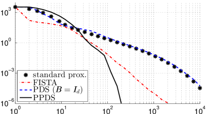
$||{\mathb{q}}^{(k)}-\widehat{{\mathb{q}}}||$

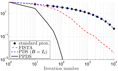
Figure 11: Criterion value (upper plots) and distance to the minimizer (lower plots) as a function of the PPDS iterations for the reconstruction problem considered in Fig. 9. The chosen initial-guess is ${\mathb{q}}^{(0)}=\textbf{0}$ for the primal variables and ${\boldsymbol{\omega}}^{(0)}=-\boldsymbol{\nabla}g({\mathb{q}}^{(0)})$ for the dual variables. The preconditioning parameter is set to $a=1$ and $(\theta,\tau,\sigma)$ were set according to the tuning rule (25). For the sake of completeness, the curve of the FISTA iterations and the PDS iterations (i.e., the PPDS equipped with the identity preconditioning matrix ${\mathb{B}}={\mathb{I}}_{d}$) are also reported.

We now illustrate the performance of the PPDS iterations for minimizing the penalized criterion involved in the joint Blind-SIM reconstruction problem shown in Fig. 9-(right). These simulations were performed with a standard MATLAB implementation of the pseudo-code shown in Algorithm 1. We set $a=1$ so that the preconditioner ${\mathb{B}}$ is the inverse of the Hessian of $g$ in (14). With this tuning, we expect that the PPDS iterations exhibit a very favorable convergence rate as long as the set of active constraints is correctly identified. Starting from initial guess ${\mathb{q}}^{(0)}=\textbf{0}$ (the dual variables being set accordingly to ${\boldsymbol{\omega}}^{(0)}=-\boldsymbol{\nabla}g({\mathb{q}}^{(0)})$, see for instance [42, Sec. 3.3]), the criterion value of the PPDS iteration depicted in Fig. 11 exhibits an asymptotic convergence rate that can be considered as super-linear. Other tunings for $a$ (not shown here) were tested and found to slow down the convergence speed. The pivotal role of the preconditioning in the convergence speed is also underlined since the PPDS algorithms becomes as slow as the standard proximal iteration when we set ${\mathb{B}}={\mathb{I}}_{d}$, see the “PDS” curve in Fig. 11. In addition, one can note from the reconstructions shown in Fig. 9 that the high-frequency components (i.e., the SR effect) are brought in the very early iterations. Actually, once PPDS is properly tuned, we always found that it offers a substantial acceleration with respect to the FISTA (or the standard proximal) iterates.

Finally, let us remind that the numerical simulations were performed with a BCCB convolution matrix ${\mathb{H}}$. In some cases, the implicit periodic boundary assumption enforced by such matrices is not appropriate and a convolution model with a zero boundary assumption is preferable, which results in a matrix ${\mathb{H}}$ with a BTTB structure. In such a case, the product of any vector by ${\mathb{H}}^{t}{\mathb{H}}$ can still be performed efficiently in $O(N\log N)$ via the FFT algorithm, see for instance [41, Sec. 5.2.3]. This applies to the computation of $\boldsymbol{\nabla}g({\mathb{q}}^{(k)})$ in the primal step (21), according to (15). In contrast, exact system solving as required by (21) cannot be implemented in $O(N\log N)$ anymore if matrix $\mathb{H}$ is only BTTB (and not BCCB). In such a situation, one can define ${\mathb{C}}$ as a BCCB approximation of ${\mathb{H}}^{t}{\mathb{H}}$, so that the preconditioning matrix ${\mathb{B}}=({\mathb{C}}+\beta{\mathb{I}}_{d})^{-1}$ remains BCCB, while ensuring that ${\mathb{B}}({\mathb{H}}^{t}{\mathb{H}}+\beta{\mathb{I}}_{d})$ has a clustered spectrum around 1 as the size $N$ increases [52, Th. 4.6].

Finally, another practical issue arises from the numerical evaluation of ${\mathcal{L}}$. No direct extension of (29d) is available when $\mathb{H}$ is BTTB but not BCCB. However, according to (25), global convergence of the PPDS iterations is still granted if $\tau<2/\widehat{{\mathcal{L}}}$ with ${\mathcal{L}}\leq\widehat{{\mathcal{L}}}$. For instance, $\widehat{{\mathcal{L}}}:=\lambda_{\text{max}}({\mathb{B}})\,(||{\mathb{H}}||_{\infty}||{\mathb{H}}||_{1}+\beta)$ is an easy-to-compute upper bound of $\mathcal{L}$.

V Conclusion

The speckle-based fluorescence microscope proposed in [1] holds the promise of a super-resolved optical imager that is cheap and easy to use. The SR mechanism behind this strategy, that was not explained, is now properly linked with the sparsity of the illumination patterns. This readily relates joint Blind-SIM to localization microscopy techniques such as PALM[13] where the image sparsity is indeed brought by the sample itself. This finding also suggests that “optimized” random patterns can be used to enhance SR, one example being the two-photon excitations proposed in this paper. Obviously, even with such excitations, the massively sparse activation process at work with PALM/STORM remains unparalleled and one may not expect a resolution with joint Blind-SIM greater than twice or three times the resolution of a wide-field microscope. We note, however, that this analysis of the SR mechanism is only valid when the sample and the illumination patterns are jointly retrieved. In other words, this article does not tell anything about the SR obtained from marginal estimation techniques that estimates the sample only, see for instance [17, 18, 19]. Indeed, the SR properties of such “marginal” techniques are rather distinct [53].

From a practical perspective, the joint Blind-SIM strategy should be tested shortly with experimental datasets. One expected difficulty arising in the processing of real data is the strong background level induced in the focal plane by the out-of-focus light. This phenomenon prevents the local extinction of the excitation intensity, hence destroying the expected SR in joint Blind-SIM. A natural approach would be to solve the reconstruction problem in its 3D structure, which is numerically challenging, but remains a mandatory step to achieve 3D speckle SIM reconstructions [10]. The modeling of the out-of-focus background with a very smooth function is possible [7] and will be considered for a fast 2D reconstruction of the sample in the focal plane.

Another important motivation of this work is the reduction of the computational time in joint Blind-SIM reconstructions. The reformulation of the original (large-scale) minimization problem is a first pivotal step as it leads to $M$ sub-problems, all sharing the same structure, see Sec. II-A. The new preconditioned proximal iteration proposed in Sec. IV-B is also decisive as it efficiently tackles each sub-problem. In our opinion, this “preconditioned primal-dual splitting” (PPDS) technique is of general interest as it yields preconditioned proximal iterations that are easy to implement and provably convergent. For our specific problem, the criterion values are found to converge much faster with the PPDS iteration than with the standard proximal iterations (e.g., FISTA). We do believe, however, that PPDS deserves further investigations, both from the theoretical and the experimental viewpoints. This minimization strategy should be tested with other observation models and prior models. For example, as a natural extension of this work, we will consider shortly the Poisson distribution in the case of image acquisitions with low photon counting rates. The global and local convergence properties of PPDS should be explored extensively, in particular when the preconditioning matrix varies over the iterations. This issue is of importance if one aims at defining quasi-Newton proximal iterations with PPDS in a general context.

References

- [1] E. Mudry, K. Belkebir, J. Savatier, E. Le Moal, C. Nicoletti, M. Allain, and A. Sentenac, “Structured illumination microscopy using unknown speckle patterns”, Nature Photonics, vol. 6, pp. 312–315, 2012.
- [2] M. Bertero and P. Boccacci, Introduction to inverse problems in imaging, Institute of Physics Publishing, 1998.
- [3] J. Goodman, Introduction to Fourier Optics, Roberts & Company Publishers, 2005.
- [4] R. Heintzmann and C. Cremer, “Laterally modulated excitation microscopy: improvement of resolution by using a diffraction grating”, in Proc. SPIE, Optical Biopsies and Microscopic Techniques III, 1999, pp. 185–196.
- [5] M. G. L. Gustafsson, “Surpassing the lateral resolution limit by a factor of two using structured illumination microscopy”, J. Microsc., 2000.
- [6] R. Ayuk, H. Giovannini, A. Jost, E. Mudry, J. Girard, T. Mangeat, N. Sandeau, R. Heintzmann, K. Wicker, K. Belkebir, and A. Sentenac, “Structured illumination fluorescence microscopy with distorted excitations using a filtered blind-SIM algorithm”, Optics Letters, vol. 38, no. 22, pp. 4723–4726, Nov 2013.
- [7] F. Orieux, E. Sepulveda, V. Loriette, B. Dubertret, and J.-C. Olivo-Marin, “Bayesian estimation for optimized structured illumination microscopy”, IEEE Trans. Im. Proc., vol. 21, no. 2, pp. 601–614, 2012.
- [8] K. Wicker, O. Mandula, G. Best, R. Fiolka, and R. Heintzmann, “Phase optimisation for structured illumination microscopy”, Opt. Express, vol. 21, no. 2, pp. 2032–2049, Jan 2013.
- [9] K. Wicker, “Non-iterative determination of pattern phase in structured illumination microscopy using auto-correlations in Fourier space”, Opt. Express, vol. 21, no. 21, pp. 24692–24701, Oct 2013.
- [10] A. Negash, S. Labouesse, N. Sandeau, M. Allain, H. Giovannini, J. Idier, R. Heintzmann, P. C. Chaumet, K. Belkebir, and A. Sentenac, “Improving the axial and lateral resolution of three-dimensional fluorescence microscopy using random speckle illuminations”, J. Opt. Soc. Am. A, vol. 33, no. 6, pp. 1089–1094, Jun 2016.
- [11] L. Condat, “A primal-dual splitting method for convex optimization involving Lipschitzian, proximable and linear composite terms”, J. Optim. Theory Appl., vol. 158, no. 2, pp. 460–479, Aug. 2013.
- [12] D. L. Donoho, A. M. Johnstone, J. C. Hoche, and A. S. Stern, “Maximum entropy and the nearly black object”, J. R. Stat. Soc., vol. 198, pp. 41–81, 1992.
- [13] E. Betzig, G. H. Patterson, R. Sougrat, O. W. Lindwasser, S. Olenych, J. S. Bonifacino, M. W. Davidson, J. Lippincott-Schwartz, and H. F. Hess, “Imaging intracellular fluorescent proteins at nanometer resolution”, Science, vol. 313, no. 5793, pp. 1642–1645, 2006.
- [14] M. J. Rust, M. Bates, and X. Zhuang, “Sub-diffraction-limit imaging by stochastic optical reconstruction microscopy (STORM)”, Nature methods, vol. 3, no. 10, pp. 793–796, 2006.
- [15] E. A. Mukamel, H. Babcock, and X. Zhuang, “Statistical deconvolution for superresolution fluorescence microscopy”, Biophys. J., vol. 102, no. 10, pp. 2391–2400, 2012.
- [16] J. Min, C. Vonesch, H. Kirshner, L. Carlini, N. Olivier, S. Holden, S. Manley, J. C. Ye, and M. Unser, “FALCON: fast and unbiased reconstruction of high-density super-resolution microscopy data”, Sci. Rep., vol. 4, no. 4577, 2014.
- [17] J. Min, J. Jang, D. Keum, S.-W. Ryu, C. Choi, K.-H. Jeong, and J. C. Ye, “Fluorescent microscopy beyond diffraction limits using speckle illumination and joint support recovery”, Scientific reports, vol. 3, 2013.
- [18] J.-E. Oh, Y.-W. Cho, G. Scarcelli, and Y.-H. Kim, “Sub-Rayleigh imaging via speckle illumination”, Opt. Lett., vol. 38, no. 5, pp. 682–684, Mar 2013.
- [19] T. Chaigne, J. Gateau, M. Allain, O. Katz, S. Gigan, A. Sentenac, and E. Bossy, “Super-resolution photoacoustic fluctuation imaging with multiple speckle illumination”, Optica, vol. 3, no. 1, pp. 54–57, 2016.
- [20] S. Labouesse, M. Allain, J. Idier, S. Bourguignon, A. Negash, P. Liu, and A. Sentenac, “Fluorescence blind structured illumination microscopy: a new reconstruction strategy”, in IEEE ICIP, Phoenix, United States, Sept. 2016.
- [21] A. Jost, E. Tolstik, P. Feldmann, K. Wicker, A. Sentenac, and R. Heintzmann, “Optical sectioning and high resolution in single-slice structured illumination microscopy by thick slice blind-SIM reconstruction”, PloS one, vol. 10, no. 7, pp. e0132174, 2015.
- [22] G. H. Golub and C. H. V. Loan, Matrix computation, The Johns Hopkins University Press, Baltimore, 3rd ed. edition, 1996.
- [23] W. Denk, J. H. Strickler, and W. W. Webb, “Two-photon laser scanning fluorescence microscopy”, Science, vol. 248, no. 4951, pp. 73–76, 1990.
- [24] M. Gu and C. J. R. Sheppard, “Comparison of three-dimensional imaging properties between two-photon and single-photon fluorescence microscopy”, J. Microsc., vol. 177, no. 2, pp. 128–137, 1995.
- [25] J. R. Lakowicz, Principles of Fluorescence Spectroscopy, Springer US, 3rd edition, 2006.
- [26] Y. Bromberg and H. Cao, “Generating non-Rayleigh speckles with tailored intensity statistics”, Phys. Rev. Lett., vol. 112, pp. 213904, May 2014.
- [27] R. Horstmeyer, R. Heintzmann, G. Popescu, L. Waller, and C. Yang, “Sub-diffraction-limit imaging by stochastic optical reconstruction microscopy (STORM)”, Nature Photonics, vol. 10, no. 2, pp. 68–71, 2016.
- [28] C. Leterrier, J. Potier, G. Caillol, C. Debarnot, F. Rueda Boroni, and B. Dargent, “Nanoscale architecture of the axon initial segment reveals an organized and robust scaffold”, Cell Reports, vol. 13, no. 12, 2015.
- [29] V. Morozov, Methods for Solving Incorrectly Posed Problems, Springer New York, 1984.
- [30] P. Hansen, “Analysis of discrete ill-posed problems by means of the L-curve”, SIAM Rev., vol. 34, pp. 561–580, 1992.
- [31] Y. Song, D. Brie, E. H. Djermoune, and S. Henrot, “Regularization parameter estimation for non-negative hyperspectral image deconvolution”, IEEE Trans. Im. Proc., vol. 25, no. 11, pp. 5316–5330, 2016.
- [32] F. Lucka, “Fast Markov chain Monte Carlo sampling for sparse Bayesian inference in high-dimensional inverse problems using L1-type priors”, Inverse Problems, vol. 28, no. 12, pp. 125012, 2012.
- [33] S. D. Babacan, R. Molina, and A. K. Katsaggelos, “Variational Bayesian blind deconvolution using a total variation prior”, IEEE Trans. Im. Proc., vol. 18, no. 1, pp. 12–26, 2009.
- [34] P. L. Combettes and V. R. Wajs, “Signal recovery by proximal forward-backward splitting”, Multiscale Model. Simul., vol. 4, no. 4, pp. 1168–1200, 2005.
- [35] A. Beck and M. Teboulle, “Gradient-based algorithms with applications to signal recovery problems”, in Convex Optimization in Signal Processing and Communications, Y. Eldar and D. Palomar, Eds., pp. 42–85. Cambridge university press, 2010.
- [36] P. L. Combettes and J.-C. Pesquet, “Proximal splitting methods in signal processing”, in Fixed-point algorithms for inverse problems in science and engineering, pp. 185–212. Springer New York, 2011.
- [37] R. T. Rockafellar, Convex analysis, Princeton university press, 1970.
- [38] A. Beck and M. Teboulle, “A fast iterative shrinkage-thresholding algorithm for linear inverse problems”, SIAM J. Imaging Sciences, vol. 2, no. 1, pp. 183–202, 2009.
- [39] P. Moulin and J. Liu, “Analysis of multiresolution image denoising schemes using generalized Gaussian and complexity priors”, IEEE Trans. Inf. Theor., vol. 45, no. 3, pp. 909–919, Sept. April 1999.
- [40] M. A. Figueiredo and R. D. Nowak, “An EM algorithm for wavelet-based image restoration”, IEEE Trans. Im. Proc., vol. 12, no. 8, pp. 906–916, 2003.
- [41] C. R. Vogel, Computational Methods for Inverse Problems, vol. 23 of Frontiers in Applied Mathematics, SIAM, 2002.
- [42] D. P. Bertsekas, Nonlinear programming, Athena Scientific, Belmont, USA, 2nd edition, 1999.
- [43] S. Bonettini, R. Zanella, and L. Zanni, “A scaled gradient projection method for constrained image deblurring”, Inverse Probl., vol. 25, no. 1, pp. 015002, 2009.
- [44] N. Pustelnik, J.-C. Pesquet, and C. Chaux, “Relaxing tight frame condition in parallel proximal methods for signal restoration”, IEEE Trans. Signal Process., vol. 60, no. 2, pp. 968–973, 2012.
- [45] S. Becker and J. Fadili, “A quasi-Newton proximal splitting method”, in Adv. Neural Inf. Process Syst., 2012, pp. 2618–2626.
- [46] H. Raguet and L. Landrieu, “Preconditioning of a generalized forward-backward splitting and application to optimization on graphs”, SIAM J. Imaging Sciences, vol. 8, no. 4, pp. 2706–2739, 2015.
- [47] E. Chouzenoux, J.-C. Pesquet, and A. Repetti, “Variable metric forward–backward algorithm for minimizing the sum of a differentiable function and a convex function”, J. Optim. Theory Appl., vol. 162, no. 1, pp. 107–132, 2013.
- [48] B. C. Vũ, “A splitting algorithm for dual monotone inclusions involving cocoercive operators”, Adv. Comput. Math., vol. 38, no. 3, pp. 667–681, Apr. 2013.
- [49] P. L. Combettes and J.-C. Pesquet, “Primal-dual splitting algorithm for solving inclusions with mixtures of composite, Lipschitzian, and parallel-sum type monotone operators”, Set-Valued Var. Anal., vol. 20, no. 2, pp. 307–330, 2012.
- [50] D. Geman and C. Yang, “Nonlinear image recovery with half-quadratic regularization”, IEEE Trans. Im. Proc., vol. 4, no. 7, pp. 932–946, July 1995.
- [51] M. Allain, J. Idier, and Y. Goussard, “On global and local convergence of half-quadratic algorithms”, IEEE Trans. Im. Proc., vol. 15, no. 5, pp. 1130–1142, May 2006.
- [52] R. H. Chan and M. K. Ng, “Conjugate gradient methods for Toeplitz systems”, SIAM Review, vol. 38, no. 3, pp. 427–482, 1996.
- [53] J. Idier, S. Labouesse, M. Allain, P. Liu, S. Bourguignon, and A. Sentenac, “A theoretical analysis of the super-resolution capacity of imagers using unknown speckle illuminations”, Research rep., IRCCyN/Institut Fresnel, 2015.