Does Eulerian percolation on percolate ?
Abstract.
Eulerian percolation on with parameter is the classical Bernoulli bond percolation with parameter conditioned on the fact that every site has an even degree. We first explain why Eulerian percolation with parameter coincides with the contours of the Ising model for a well-chosen parameter . Then we study the percolation properties of Eulerian percolation. Some key ingredients of the proofs are couplings between Eulerian percolation, the Ising model and FK-percolation.
Key words and phrases:
Eulerian percolation, Ising model, percolation with degree constraints.2000 Mathematics Subject Classification:
60K35, 82B43.1. Introduction
Eulerian percolation with parameter on the edges of a finite graph is the classical independent Bernoulli percolation with parameter on its edges, but conditioned to be even, i.e. conditioned to the fact that each vertex of the graph has an even number of open edges touching it. In this paper, we aim to study the percolation properties of the Eulerian (or even) percolation on the edges of . This paper has two parts.
1. On , the event by which we want to condition has probability . The first step is thus to define properly the Eulerian percolation measures on the edges of , by the mean of specifications in finite boxes and of Gibbs measures. Doing so, the Eulerian percolation measure with parameter is given by the contours of the Ising model on the sites of the dual for a well-chosen parameter :
Theorem 1.1.
For every , there exists a unique even percolation measure on the edges of with opening parameter , and we denote it by . It is the image by the contour application of any Gibbs measure for the Ising model on the dual graph of , with parameter
Moreover, is invariant and ergodic under the natural action of .
Note that Eulerian percolation with parameter , resp. , corresponds to the contours of the Ising model in the ferromagnetic range , resp. antiferromagnetic range . Theorem 1.1 is an extension of Theorem 5.2 of Grimmett and Janson [9], that studies random even subgraphs on finite planar graphs. In the same paper, they mention the existence of a thermodynamic limit, but the question of uniqueness is not asked.
2. We are interested in the probability, under the even percolation measure , of the percolation event
Our first result consists in proving the almost-sure uniqueness of the infinite cluster when it exists:
Theorem 1.2.
For every , there exists -almost surely exactly one infinite cluster or -almost surely no infinite cluster.
Note that the “even degree” condition induces correlations between states of edges, that break the classical finite energy property. However, we can adapt the classical proof by using the interpretation in terms of contours of the Ising model. To study the percolation itself, we have at our disposal the results proved for the Ising model on , especially in the ferromagnetic range. Remember that is the critical value of the Ising model in ; we introduce the corresponding percolation parameter
We prove the following:
Theorem 1.3.
In terms of even percolation with parameter ,
-
•
for every , ,
-
•
for every , .
In terms of the Ising model with parameter , these results correspond to:
-
•
for , for every Gibbs measure with parameter , contours a.s. do not percolate,
-
•
for such that , for every Gibbs measure with parameter , contours a.s. percolate.
These results are summarized in the following table:
We did not manage to settle the case (corresponding to for the Ising model). In independent Bernoulli bond percolation, is non-decreasing, and this follows from a natural coupling of percolation for all parameters . The same monotonicity occurs for FK percolation with parameter . This is strongly related to the fact that FK percolation satisfies the FKG inequality. Here, conditioning by the Eulerian condition breaks the association, even if the underlying graph is Eulerian. See Section 5 for an example of the strange things that may happen. We naturally conjecture that is indeed the unique percolation threshold for Eulerian percolation on :
Conjecture 1.4.
In terms of even percolation: .
In terms of the Ising model: for every Gibbs measure with parameter , contours a.s. percolate.
The percolation results for essentially follow from the results about percolation of colors in the Ising model in the ferromagnetic case . The Ising model in the antiferromagnetic case has been much less studied, so other kinds of arguments are needed for .
In order to settle the case , we introduce a coupling between and . This coupling has the property to increase the connectivity, so that percolation for implies also percolation for .
The case for follows from the link between the Ising model and FK percolation. A stochastic comparison between even percolation with a large parameter and independent percolation with a large parameter gives the result for , and we only sketch the extension of that proof to , using techniques from Beffara and Duminil-Copin [2].
2. Eulerian percolation probability measures
On , we consider the set of edges between vertices at distance for . An edge configuration is an element if , the edge is present (or open) in the configuration , and if , the edge is absent (or closed). For , we define the degree of in the configuration by setting
An Eulerian edge configuration is then an element of
If and , we denote by the concatenation of the configuration restricted to and of the configuration restricted to .
Gibbs measures for Eulerian percolation
For each finite subset of and each function on , we can define
| (1) |
Note that is Feller, in the following sense: is continuous (for the product topology) as soon as is continuous. A standard calculation gives
We denote by the probability measure on that is such that, for each bounded measurable function ,
A probability measure on is said to be a Gibbs measure for Eulerian percolation (or a Eulerian percolation probability measure) if one has
-
•
-
•
For each continuous fonction on , for each finite subset of ,
(2)
We denote by the set of Gibbs measures for Eulerian percolation with opening parameter .
Colorings with two colors and Eulerian percolation
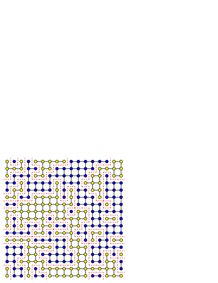
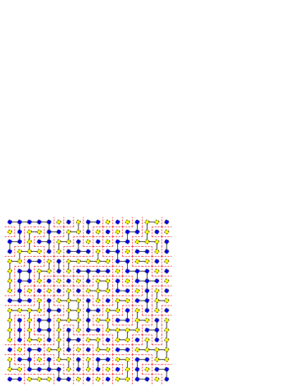
A natural way to obtain a Eulerian configuration of the edges of a planar graph is to take the contours of a coloring in two colours of the sites of its dual, and this is what we decribe now in the case.
Let be the dual graph of . The set of edges of is the image of by the translation with respect to the vector . If , we denote by its dual edge, i.e. the only edge in that intersects . We can map any coloring of the sites of with the two colors and to its contour in the following way:
Let us see that . Indeed, set , and fix . Let be the four corners of the square with length side in whose center is : then the four edges issued from are the dual edges of , , and . Thus
So .
Reciprocally, the dual of a planar Eulerian graph is bipartite (see for instance Wilson and Van Lint [16], Theorem (34.4)), and there are exactly two ways of coloring the sites of a connected bipartite graph with two colors in such a way that the extremities of every edge are in different colors. In our case, fix a Eulerian edge configuration . By setting , and for any , equals (-1) power the number of edges in crossed by any path (in the dual) between and , we properly define a coloring of , and Finally, the contour application is surjective and two-to-one.
As we will see now, the Gibbs measures for Eulerian percolation can be obtained as the images by the contour application of the Gibbs measures for the Ising model in .
Gibbs measures for the Ising model on
It is of course the same model as the Ising model on , but to avoid confusion between the initial graph and its dual in the sequel, we present it directly in the dual . Fix a parameter . For a finite subset of , the Hamiltonian on is defined by
Then, we can define, for each bounded measurable function ,
For each , we denote by the probability measure on which is associated to the map . When , colors of sites inside are i.i.d. and follow the uniform law in . When , neighbour sites prefer to be in the same color (ferromagnetic case), while when , neighbour sites prefer to be in different colors (anti-ferromagnetic case).
A Gibbs measure for the Ising model on with parameter is any probability measure on such that for each continuous function, for each finite subset of ,
We denote by the set of Gibbs measures for the Ising model with parameter . The Ising model presents a phase transition: set (see Onsager [14]), then
-
•
if , then there is a unique Gibbs measure;
- •
For , the Gibbs measures are obtained from by changing the colors on the subset of even sites. In other words, if
then belongs to if and only if . For the details, see Chapter 6 in Georgii [6].
 |
 |
Proof of Theorem 1.1, existence
We first prove the existence of Gibbs measure for Eulerian percolation. Let us define and denote by the set of edges such that has at least one end in . Since is a closed subset of the compact set , the sequence has a limit point with . Using Equation (1) and the fact that is Feller, it is easy to see that , which is therefore not empty.
This proof is not surprising for people who are familiar to the general theory of Gibbs measures, as described in Georgii [6]. Nevertheless, it must be noticed that is not defined on the whole set (it is not a specification in the realm of Georgii [6]), which leads us to mimic a standard proof.
To prove the uniqueness of the even percolation probability measure, we first need the following lemma:
Lemma 2.1.
Let and with . Suppose that is a simply connected subset of , and denote by the set of edges such that has at least one end in .
Fix and set . Then, the probability is the image of under the contour application .
Proof.
By construction, the image of under the map is concentrated on configurations that coincide with outside . Obviously it is the same for , so we must focus on the behaviour of the edges in .
Let be such that and coincide outside . There are exactly two colorings such that . If and are two neighbours in , then
so . Since is connected, it follows that one of the two colorings, say , coincides with on (and with ). Thus and , and:
Since we compare probability measures with the same support, . ∎
Proof of Theorem 1.1, uniqueness
Let us now see that all Gibbs measures for the Ising model with parameter have the same image by the application . Let : there exists such that . Remember that is the image of by the exchange of colors, that leaves the contours unchanged. So, if ,
Let and set as before . Let be a continuous function on , and let us prove that for each ,
With Equation (2), it will imply by dominated convergence that
and thus that is the image by the application of , or of any Gibbs measure for the Ising model with parameter .
Let be an Eulerian edge configuration, and let be such that . Let be a limiting value of . By extracting a subsequence if necessary, we can assume that converges to , which is then in , and that . By Lemma 2.1,
To conclude, note that is stationary and ergodic, and so does .
3. Unicity of the infinite cluster in Eulerian percolation
Proof of Theorem 1.2.
Since is ergodic and is a translation-invariant event, it is obvious that . To prove the unicity of the infinite cluster, we now follow the famous proof by Burton and Keane [3]. The main point here is that the Eulerian percolation measure does not satisfy the finite energy property: once a configuration is fixed outside a box, the even degree condition forbids some configurations inside the box. But the Ising model has the finite energy property, and we will thus use the representation of even percolation in terms of contours of the Ising model.
The number of infinite clusters is translation-invariant, so the ergodicity of implies that it is -almost surely constant: there exists such that . The first step consists in proving that . So assume for contradiction that is an integer larger than . Consider a finite box , large enough to ensure that with positive probability (under ), the box intersects at least two infinite clusters. Using Theorem 1.1, this implies that with positive probability (under for the parameter corresponding to ), the contours of the Ising model present two infinite connected components that intersect . But the Ising model has the finite energy property: by forcing the colors inside to be a chessboard, we keep an event with positive probability, and we decrease the number of infinite clusters in the contours by at least one. Coming back to Eulerian percolation, this gives , which is a contradiction. See [13, 12] for the first version of such an argument.
In the final step, we prove that is impossible. Assume by contradiction that . We work now with the colorings of the sites of , under .
By taking large enough, we can assume that the event “the box intersects at least infinite clusters” has positive probability. Let be a coloring of the sites in such that
Take in this event. Each infinite cluster intersecting crosses via an open edge, and this edge sits between a site and a site.
Thus the distinct infinite (edge) clusters intersecting imply the existence of at least clusters of vertices in . To avoid geometric intricate details, we do not want to consider -clusters in that are in the corners: we thus remove from our clusters at most clusters (the one containing the corner if it is a , and the nearest cluster on each side). We are now left with at least disjoint -clusters in , sitting near edges of distinct infinite clusters: they are far away enough so that we can draw, inside , paths of sites linking these three clusters to three of the four centers of the sides of , in such a way that two distinct paths are not -connected. See Figure 2.
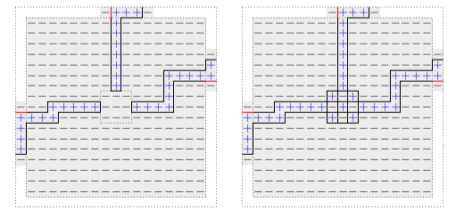
Consider now the following coloring of : all sites in the three paths are , all the other sites are . With this coloring, intersects exactly three infinite clusters of open edges. If we change the coloring of in a chessboard, intersects exactly one infinite cluster of open edges. In this case, we say that is a trifurcation. As has finite energy, we see that the probability that is a trifurcation has positive probability, and the end of the proof is as in Burton-Keane.
4. Percolation properties of Eulerian percolation
The proof of Theorem 1.3 is split into five steps: Lemmas 4.1, 4.2, 4.3, 4.5 and 4.7, that are respectively considering the ranges , , and .
4.1. The ferromagnetic zone of the Ising model: .
Lemma 4.1.
For , .
Proof.
Let be a spin configuration of , and let be the even subgraph of made of the contours of .
We need here the notion of -neighbours: two sites are -neighbours if and only if . A -chain is then a sequence of sites in such that two consecutive sites are -neighbours.
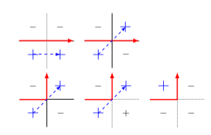
Let us assume that contains an infinite path . For each edge along , there is a spin in the configuration on one side of that edge, and a spin on the other side. The set of spins (resp. ) in along constitutes an infinite -chain of spins (resp. ), as illustrated in Figure 3, which shows the evolution of the -chain of spins for the different possible steps taken by . Set
Lemma 4.2.
At the critical point , we have: .
The proof of this lemma will follow from the stochastic comparison between even percolation and the random cluster model stated in Lemma 4.6, and can be found just after Lemma 4.7. The argument, extended to , also gives an alternative proof of Lemma 4.1.
Lemma 4.3.
For , .
Proof.
Let us set
Let , and let be an infinite -chain of spins in . For each spin along , let us consider the cluster of spins to which it belongs. Since , these clusters are finite. The union of the contours of these clusters is an infinite connected subgraph of . Indeed, let be the coordinates of two consecutive spins of the -chain . If and are not in the same cluster of spins , it means that the step from to in is diagonal (with spins in the opposite diagonal), and that the contours of the clusters of and meet at point . Thus, any two consecutive points of are such that the contours of their clusters are connected (or possibly the same). By induction, one can then prove that the union of the contours of all the clusters of spins of is a connected subgraph of .
4.2. The antiferromagnetic zone of the Ising model:
This is the most complex case, because the geometry of the antiferromagnetic Ising model is less well known.
4.2.1. Percolation for
We want here to build, for , a coupling between and that increases connectivity:
Lemma 4.4.
Let . The law of the field under is stochastically dominated by the law of the field under .
By Lemma 4.3, there is percolation under for , so we deduce:
Lemma 4.5.
For , .
Proof of Lemma 4.4.
For every site , we consider the set of its four surrounding edges, i.e. the four edges of the unit square with center . Define . Then is the disjoint union of the for .
We define . A point encodes two configurations of the four edges surrounding : and .
For let us set .
1. We first define a probability measure on , whose first marginal is , and whose second marginal is . This probability is defined by the table below, and has the property that -almost surely, either , or the configuration is the complement of , which can be interpreted as the flip of the spin at . This is possible since for any ,
In particular, is such that there are the following possibilities for :
-
•
with probability , we have ,
-
•
with probability , we have ,
-
•
with probability , we have .
| probability under | number of cases | |||
|
|
1 | |||
|
|
1 | |||
|
|
1 | |||
|
|
||||
|
|
||||
|
|
||||
|
|
Because and thus , the probability measure is well defined. One can easily check that has the following properties.
-
(P1)
The law of under is , and the law of under is .
-
(P2)
is more connected than : -almost surely, if two corners of the squares are connected in , then they are connected in .
-
(P3)
-almost surely, the parity of the degree of each corner of the square is the same in the two configuration and .
Note however that the coupling is not increasing: with probability , and are not comparable.
2. We now extend the previous coupling to finite boxes of . Define, for , and denote by the subset of edges such that has at least one end in . Then is the disjoint union of the for . Set .
Thus, is a probability measure on , where encodes two edges configurations on the whole plane: and . From Properties (P1), (P2) and (P3), one gets:
-
(P1’)
The law of under is , and the law of under is .
-
(P2’)
almost surely, if then .
-
(P3’)
almost surely, .
3. Now we want to condition by the event that both configurations and are even. By Property (P3’), we have
Remember the definition of . With Property (P1’), one gets
In the same manner, . And we obtain
-
(P1”)
The law of under is , and the law of under is .
-
(P2”)
almost surely, if then .
4. It remains to take limits when goes to . We can extract a subsequence such that converges to a probability measure when tends to infinity. Thus both marginals and also converge when tends to infinity to the marginals of . As in the proof of Theorem 1.1, their limits are Gibbs measures for even percolation, so by uniqueness, they respectively converge to and . Thus,
-
(P1”’)
The law of under is , and the law of under is .
-
(P2”’)
almost surely, if then .
So the law of the field under is stochastically dominated by the law of the field under . ∎
4.2.2. Percolation for
In the following, we give a full proof of the fact that percolation occurs for , and give some hints about the way to prove that there is percolation for .
The proof is based on a coupling between the Ising model and the random cluster (or FK-percolation) model. We just recall a few results on the random cluster model, and refer to Grimmett’s book [8] for a complete survey on this model.
The random cluster measure with parameters and on a finite graph is the probability measure on defined by:
where is the number of connected components in the subgraph of given by , and is a normalizing constant.
On , it is known that at least for , there exists a unique infinite volume random cluster measure, that we denote by (Theorem (6.17) in [8]). It is a probability measure on . In our study of even percolation, we use two properties of the random cluster model: its link with the Ising model, and its duality property. For , let us set
(Q1) From a spin configuration whose distribution is any Gibbs measure for the Ising model with parameter , one obtains a subgraph with distribution by keeping independently each edge between identical spins with probability , and erasing all the edges between different spins. For finite graphs, this can be found in Theorem (1.13) in [8]. For the case, Theorem (4.91) in [8] says that this erasing procedure allows to couple the wired boundary infinite volume random cluster measure and the Ising measure on .
For a subgraph , we denote by the complementary subgraph of , meaning that the open edges of are exactly the closed edges of . We denote by the dual graph of : in , the edge is open if and only if is closed. Let us point out that : we thus simply denote this graph by . We naturally extend these notations to measures.
(Q2) The random cluster model has the following duality property (Theorem (6.13) in [8]): if is distributed according to , then the distribution of is equal to , where:
Let us also recall that the measure on the edges of is obtained as the contours of any Ising measure with parameter on , and in particular as the contours of (Theorem 1.1). Using these facts, we will prove the following proposition.
Lemma 4.6.
For , we have the following stochastic ordering:
Proof.
For , starting from an Ising configuration of distribution , let us draw all the edges between identical spins. By Theorem 1.1, the configuration on the edges of that we obtain is distributed according to .
By property (Q1) above, this measure on the edges of stochastically dominates the distribution :
see Figure 4 for an illustration.
Ising model
| Random cluster | Even percolation |
Taking the dual of graphs, we obtain:
with, by property (Q2), with
Thus, . Taking the complementary of configurations, we obtain the second stochastic comparison. ∎
In particular, if for some parameter , there is percolation of closed edges in the random cluster model , then there is percolation of open edges for .
Let us set
The event is non-increasing, and is stochastically increasing (Theorem (3.21) in [8]), so the map is non-increasing: there exists a critical value such that for and for . In words, is the critical parameter for percolation of closed edges in the random cluster model. As a consequence of Lemma 4.6, we obtain the following result.
Lemma 4.7.
For , .
Proof.
By definition of and with Lemma 4.6, if , which is equivalent to . We conclude with the 0–1 law. ∎
As it was first derived by Onsager [14], the critical parameter for percolation of open edges in the random cluster model is equal to the self-dual point, i.e. the only fixed point of the map : thus
Proof of Lemma 4.2.
We now give a complete and easy proof of the fact that and a sketch of proof that the strategy used by Beffara and Duminil-Copin [2] to prove that the self-dual point of FK-percolation coincides with the critical point may be adopted here.
Lemma 4.8.
.
Proof.
The probability measure is dominated by a product of Bernoulli measures with parameter (Theorem (3.21) in [8]) and for , the event has a positive probability under the product of Bernoulli measures with parameter . As is a non-increasing event, the lemma follows. ∎
Lemma 4.9.
Sketch of proof.
The proof by Beffara and Duminil-Copin [2] is based of three kind of arguments:
-
•
The study of the variation of with respect to .
-
•
The self-duality property
-
•
The FK measures are strongly associated
It is obvious that the self-duality property works as well for closed bonds as for open bonds. Also, the strong association of the closed bonds of FK-percolation immediately follows from the strong association of the open bonds. The study of the variation of the probabilities with respect to uses the methods that are described in the monography by Grimmett [8]. It does not depend on the reference measure: they can be applied as well with (FK percolation) as with (percolation of the closed bonds of FK percolation). ∎
From Lemma 4.7, the inequality then implies that for , while implies that for .
5. Association and monotonicity under the Eulerian condition
The study of Bernoulli bond percolation on a graph intensively uses the following properties of the product measure :
-
•
monotonicity: for every increasing event , the map is non-decreasing.
-
•
association: for every pair of increasing event , ,
or, equivalently, for every pair of non-decreasing bounded functions , , we have .
It is natural to ask if these properties could be preserved for the measure
In the following, we investigate the case of the particular undirected finite Eulerian graph given by Figure 5: we show that the monotonicity property is preserved whereas the association property is lost. Note that every vertex in has even degree.
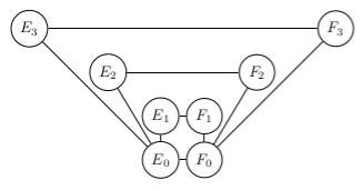
For simplicity, we denote the Eulerian percolation measure on with opening parameter .
For each , set and . It is not difficult to see that is entirely determined by
| (3) |
where and is the normalizing constant:
For , set . These events have the same probability
The events , , , coincide -almost-surely, so and are positively correlated. But
for , so and are negatively correlated for each .
However, the sequence is non-decreasing for the stochastic order:
Theorem 5.1.
Let be the graph illustrated by Figure 5. Let be an increasing event. Then, is non-decreasing. Equivalently, if is a monotonic boolean function on , is non-decreasing.
Proof.
Let be the state of the edge between vertices and . The structure of the graph implies that -almost surely,
So, if is a non-decreasing fonction on , we have a.s. :
By construction, is a non-decreasing function, so it is sufficient to prove that for any non-decreasing function :, the map is non-decreasing. The law of under is easy to express: for every
With (3), it is easy to see that can be expressed as a rational function of :
so if is sufficient to check that the polynomial has no positive root, which can be easily performed with a modern computer. In fact, it happens that for each monotonic boolean functions ,
In most cases, the coefficients of are non-negative; in any case, it is easy to prove that has no positive root.
We obtain the list of the 168 functions by a brute-force algorithm based on the following remark: if denotes the set of monotonic boolean functions on , there is a natural one-to-one correspondance between and : a function of variables is associated to the pair of functions . The number of monotonic boolean functions is known as the Dedekind number. The sequence increases very fast and is not easy to compute. In fact, the exact values are only known for (see Wiedemann [17]). ∎
We conjecture that this result should be more general:
Conjecture 5.2.
Let be a Eulerian graph. Then, the sequence of Eulerian percolation measures on is stochastically non-decreasing.
Note that Cammarota and Russo [4] proved related results supporting this conjecture.
Appendix: code of the Julia program
References
- [1] Michael Aizenman. Translation invariance and instability of phase coexistence in the two-dimensional Ising system. Comm. Math. Phys., 73(1):83–94, 1980.
- [2] Vincent Beffara and Hugo Duminil-Copin. The self-dual point of the two-dimensional random-cluster model is critical for . Probab. Theory Related Fields, 153(3-4):511–542, 2012.
- [3] R. M. Burton and M. Keane. Density and uniqueness in percolation. Comm. Math. Phys., 121(3):501–505, 1989.
- [4] Camillo Cammarota and Lucio Russo. Bernoulli and Gibbs probabilities of subgroups of . Forum Math., 3(4):401–414, 1991.
- [5] Antonio Coniglio, Chiara Rosanna Nappi, Fulvio Peruggi, and Lucio Russo. Percolation and phase transitions in the Ising model. Comm. Math. Phys., 51(3):315–323, 1976.
- [6] Hans-Otto Georgii. Gibbs measures and phase transitions, volume 9 of de Gruyter Studies in Mathematics. Walter de Gruyter & Co., Berlin, 1988.
- [7] Hans-Otto Georgii and Yasunari Higuchi. Percolation and number of phases in the two-dimensional Ising model. J. Math. Phys., 41(3):1153–1169, 2000. Probabilistic techniques in equilibrium and nonequilibrium statistical physics.
- [8] Geoffrey Grimmett. The random-cluster model, volume 333 of Grundlehren der Mathematischen Wissenschaften [Fundamental Principles of Mathematical Sciences]. Springer-Verlag, Berlin, 2006.
- [9] Geoffrey Grimmett and Svante Janson. Random even graphs. The Electronic Journal of Combinatorics [electronic only], 16(1):Research Paper R46, 19 p.–Research Paper R46, 19 p., 2009.
- [10] Y. Higuchi. On the absence of non-translation invariant Gibbs states for the two-dimensional Ising model. In Random fields, Vol. I, II (Esztergom, 1979), volume 27 of Colloq. Math. Soc. János Bolyai, pages 517–534. North-Holland, Amsterdam-New York, 1981.
- [11] Yasunari Higuchi. Coexistence of infinite -clusters. II. Ising percolation in two dimensions. Probab. Theory Related Fields, 97(1-2):1–33, 1993.
- [12] C. M. Newman and L. S. Schulman. Infinite clusters in percolation models. J. Statist. Phys., 26(3):613–628, 1981.
- [13] C. M. Newman and L. S. Schulman. Number and density of percolating clusters. J. Phys. A, 14(7):1735–1743, 1981.
- [14] Lars Onsager. Crystal statistics. I. A two-dimensional model with an order-disorder transition. Phys. Rev. (2), 65:117–149, 1944.
- [15] Lucio Russo. The infinite cluster method in the two-dimensional Ising model. Communications in Mathematical Physics, 67(3):251–266, 1979.
- [16] J. H. van Lint and R. M. Wilson. A course in combinatorics. Cambridge University Press, Cambridge, second edition, 2001.
- [17] Doug Wiedemann. A computation of the eighth Dedekind number. Order, 8(1):5–6, 1991.