Novel Performance Analysis of Network Coded Communications in Single-Relay Networks

Abstract

In this paper, we analyze the performance of a single-relay network in which the reliability is provided by means of Random Linear Network Coding (RLNC). We consider a scenario when both source and relay nodes can encode packets. Unlike the traditional approach to relay networks, we introduce a passive relay mode, in which the relay node simply retransmits collected packets in case it cannot decode them. In contrast with the previous studies, we derive a novel theoretical framework for the performance characterization of the considered relay network. We extend our analysis to a more general scenario, in which coding coefficients are generated from non-binary fields. The theoretical results are verified using simulation, for both binary and non-binary fields. It is also shown that the passive relay mode significantly improves the performance compared with the active-only case, offering an up to two-fold gain in terms of the decoding probability. The proposed framework can be used as a building block for the analysis of more complex network topologies.

I Introduction

Random Linear Network Coding (RLNC) has been originally proposed by R. Ahlswede et al. [1] as a way to improve the communication throughput over a wired multi-hop network. Nowadays, the RLNC principle is being applied in several application domains [2]. This paper focuses on the adoption of RLNC as a way to improve the reliability over a network [3, 4]. The principle underneath that RLNC application has been presented in [3] and can be summarized as follows. Instead of directly transmitting a set of source packets, the source node generates and transmits a stream of coded packets to one or more destination nodes. Each coded packet is obtained as a linear combination of the source packets. The destination nodes recover the set source packets as soon as they collect a number of linearly independent coded packets equal to the number of the source packets.

Generally, multi-hop relay networks interconnecting one or more source nodes to several destination nodes have been extensively investigated [5, 6, 7]. In particular, [5, 6] refer to system models where a source node transmits a packet stream to multiple destination nodes, via several intermediate relay nodes. In that tree-based topology, network flows are combined by the relay nodes to achieve the min-cut max-flow [2] between the source and each destination node. In fact, [5, 6] only refer to the classic binary RLNC principle as a way to efficiently combine network information flows. Unlike [5] and [6], [7] characterizes the performance of a multi-relay network where RLNC operations are performed over a generic Galois Field (GF) composed by an arbitrary number of elements. Also in that case, we observe that [7] refers to a tree-based network topology as in [5, 6]. Differently from [5, 6, 7], our system model adopts the RLNC principle as a way to improve communication reliability. Hence, both the source and relay nodes are supposed to transmit streams of coded packets towards the destination node.

The RLNC principle has also been adopted in more complex network topologies, which may not necessarily resemble a direct acyclic graph, such as a mobile ad-hoc network [8, 9]. In that case, intermediate nodes are supposed to combine multiple incoming network flows and typically relay one combined flow towards the next intermediate node or the destination node. Also in this application domain, the goal is that of achieving the min-cut max-flow and not that of improving the reliability of communications. Another key difference between the aforementioned papers and ours is that we assume that the source node can communicate with the destination node directly, not only via a relay node. In other words, we refer to a system model where the destination node can be both a one-hop and two-hop neighbour of the source node, which can be observed in some “casual” domestic network deployments [10].

Similar to our RLNC application over a relay network is what has been proposed in [11]. In that paper, the source node transmits streams of coded packets to both a relay node and destination nodes. However, the relay node transmits a newly generated stream of coded packets only if it can recover what has been previously transmitted by the source node. Unlike [11], if the relay node has not been able to recover the original source message, we assume that it simply relays the set of coded packets that it has been able to collect. In the reminder of the paper, we will show how that improves the overall communication reliability by up to two times. We also observe that [11] provides an approximated performance model. Even though we refer to a simpler system model, we derive a novel theoretical framework for a single-relay network, which is exact for any GF, and explicitly adopts the RLNC principle as a way to improve communication reliability. The result can be used as a building block for the analysis of more complex networks.

The paper is organized as follows. Section II presents the considered system model. Section III describes the proposed theoretical framework based on an exact performance characterization of RLNC over a broadcast network topology. Numerical results are presented in Section IV, while our conclusions are drawn in Section V.

II System Model and Background

Fig. 1: Block diagram of a single-user single-relay network with packet error probabilities $p_{SD}$, $p_{SR}$ and $p_{RD}$.

A single-user single-relay network is depicted in Fig. 1. The network consists of a source node $S$, relay $R$ and destination $D$, and the goal is to transmit a message comprising of $K$ equal-size packets from $S$ to $D$. To this end, the source node encodes the $K$ message packets by using RLNC, such that each coded packet is a linear combination of the original packets with the coefficients drawn uniformly at random over a $GF(q)$, where $q$ is the field size. In total, $S$ transmits $N_{S}\geq K$ coded packets. As proposed in [12], we assume that all receiving nodes have a knowledge of seeds used to generate the coded packets they receive, such that the coding vector of each packet can be re-generated.

Let $p_{SD}$, $p_{SR}$ and $p_{RD}$ denote the Packet Error Probabilities (PEPs) of the links connecting $S$ with $D$, $S$ with $R$, and $R$ with $D$, respectively. As is traditional in relay networks, the communication is performed in two stages. At the first stage, $S$ transmits coded packets to $R$ and $D$. Both $R$ and $D$ receive a number of packets, for which they can restore the corresponding coding vectors. The latter are stacked together horizontally to form an $M_{R}\times K$ coding matrix $\mathbf{C}_{R}$ at the relay node and an $M_{D}\times K$ coding matrix $\mathbf{C}_{D}$ at the destination node. Since $R$ and $D$ may receive the same packets from $S$, the matrices may have common rows. Let $M_{RD}$ denote the number of such common rows. At this point, the destination may have enough coding packets to make its coding matrix $\mathbf{C}_{D}$ full-rank, thus being able to decode the original message without any assistance from $R$.

At the second stage, it is checked if the relay coding matrix $\mathbf{C}_{R}$ is full rank. If so, $R$ decodes the original $K$ packets and re-encodes them using newly generated random coefficients from $GF(q)$ into $N_{R}$ packets and transmits them to $D$. In general, $N_{R}\neq N_{S}$. We call this case the active relay mode. If the relay node cannot decode the source packets, it simply re-transmits the $M_{R}$ packets to the destination node, which corresponds to the passive relay mode. In either mode, we denote $M_{D}^{\prime}$ as the number of coding vectors reached $D$ from $R$, and $\mathbf{C}_{D}^{\prime}$ as the updated $M_{D}+M_{D}^{\prime}\times K$ coding matrix at $D$.

The described relay network is different from the one proposed previously in [11], since in the latter the relay node transmits only if it can decode packets from the source node. Naturally, the passive relay mode should improve the decoding probability at $D$ in cases when $R$ fails to decode. In addition, the described system and its analysis can be straightforwardly extended to a network with multiple sources, in which each source has an independent communication channel. This again contrasts with [11], where the relay node uses packets from both sources at the encoding stage, thus introducing correlation between the sources.

II-A Theoretical Background

We now provide some background results on RLNC which we will use in our analysis.

The number of full-rank $m\times k$ matrices generated over $GF(2)$, with $m\geqslant k$, is given by [13]

$$F(m,k)=\prod_{i=0}^{k-1}(2^{m}-2^{i})=2^{mk}\prod_{i=0}^{k-1}(1-2^{i-m}).$$ (1)

Based on that, the number of matrices of the same size that have rank $r\leq k$ can be calculated as

$$G(m,k,r)=\frac{F(m,r)F(k,r)}{F(r,r)}.$$ (2)

The probability of a random $m\times k$ matrix having full rank can be obtained by dividing (1) by the number of all possible $m\times k$ matrices:

$$\mathbb{P}(m,k)\triangleq 2^{-mk}F(m,k).$$ (3)

Similarly, the probability of a random $m\times k$ matrix having rank $r\leq k$ is given by

$$\mathbb{P}_{r}(m,k)\triangleq 2^{-mk}G(m,k,r).$$ (4)

In a general case, when the elements are generated from $GF(q)$, $q\geq 2$, (3) can be rewritten by simply replacing $2$ with $q$ (see, for example, [4]):

$$\mathbb{P}(m,k)=\prod_{i=0}^{k-1}(1-q^{i-m}).$$ (5)

Furthermore, following the same train of thought used to obtain (2) in the binary case, the probability (4) can be generalized to the non-binary case as follows:

$$\mathbb{P}_{r}(m,k) = q^{-mk}G(m,k,r)$$

$$= \frac{1}{q^{(m-r)(k-r)}}\prod_{i=0}^{r-1}\frac{(1-q^{i-m})(1-q^{i-k})}{1-q^{i-r}}.$$

Consider now the application of RLNC to a point-to-point link, with a source node encoding $K$ source packets and transmitting $N$ coded packets to the destination. The probability of successful decoding for such link characterized by the PEP $p$ can be given by [11]

$$P_{ptp}(N,K,p)=\sum_{M=K}^{N}B(M,N,p)\mathbb{P}(M,K),$$ (7)

where $B(M,N,p)$ is the probability mass function (PMF) of the binomial distribution:

$$B(M,N,p)=\binom{N}{M}(1-p)^{M}p^{N-M}.$$ (8)

In addition to the binomial distribution, we will also need its generalized version - the multinomial distribution [14]. The PMF of such distribution describes the probability of a particular combination of numbers of occurrences of $k$ possible mutually exclusive outcomes out of $n$ independent trials and is given by

$$f(\mathbf{x};n,\mathbf{\theta})=\alpha(\mathbf{x})\theta_{1}^{x_{1}}\cdots\theta_{k}^{x_{k}},\quad\mathrm{for}\,\sum_{i=1}^{k}x_{i}=n,$$ (9)

where $\mathbf{x}=(x_{1},\ldots,x_{k})$ is a combination of numbers of occurrences, such that the sum of them equals $n$, ${\mathbf{\theta}=(\theta_{1},\ldots,\theta_{k})}$ are probabilities of each outcome and

$$\alpha(\mathbf{x}) = \frac{n!}{x_{1}!x_{2}!\ldots x_{k}!}$$ (10)

$$= \binom{n}{x_{1}}\binom{n-x_{1}}{x_{2}}\ldots\binom{n-\sum_{i=1}^{k-2}x_{i}}{x_{k-1}}$$

is the multinomial coefficient.

III Proposed Theoretical Framework

Our goal is to derive the probability of successful decoding for the single-relay network described in the previous section. In contrast with [11], we aim to derive the exact formulation, by taking into account the fact that the coding matrices of $R$ and $D$ are correlated due to the presence of common rows. But first, we establish some preliminary results.

III-A Preliminaries

Consider a block matrix $\mathbf{X}$ composed of two vertically concatenated random matrices $\mathbf{A}$ and $\mathbf{B}$ with dimensions $a\times k$ and $b\times k$ generated over $GF(q)$:

$$\mathbf{X}=\left(\begin{array}[]{c}\mathbf{A}\\ \mathbf{B}\end{array}\right).$$ (11)

Corollary 1.

The probability of matrix $\mathbf{X}$ being full-rank is given by

$$\Pr[\mathrm{rank}\,\mathbf{X}=k]=\sum_{i=\max(0,k-b)}^{\min(a,k)}\mathbb{P}_{i}(a,k)\mathbb{P}(b,k-i).$$ (12)

Proof:

This corollary is based on Theorem 2 in [13], where the authors proved the result for a more general case, when $\mathbf{X}$ is a block angular matrix. Here, we follow the same train of thought. Suppose that $\mathbf{A}$ has rank $i$ which is upper-bounded by its smallest dimension, and hence has $i$ linearly independent columns. $\mathbf{X}$ is then full-rank if $\mathbf{B}$ has $k-i$ linearly independent columns, with the rest of its columns selected in an arbitrary way. The number of ways $\mathbf{A}$ can be chosen to have rank $i$ is $G(a,k,i)$. The $k-i$ linearly independent columns of $\mathbf{B}$ can be selected in $F(b,k-i)$ ways, while the $i$ arbitrary columns of $\mathbf{B}$ can be selected in $q^{ib}$ ways. Finally, the total number of possible matrices $\mathbf{X}$ is $q^{(a+b)k}$. This yields the following:

$$\Pr[\mathrm{rank}\,\mathbf{X}=k] {}={} q^{-(a+b)k}\sum_{i}G(a,k,i)F(b,k-i)q^{ib}$$ (13)

$${}={} \sum_{i}q^{-ak}G(a,k,i)q^{-b(k-i)}F(b,k-i)$$

$${}={} \sum_{i}\mathbb{P}_{i}(a,k)\mathbb{P}(b,k-i).$$

The starting value of $i$ in the summation is based on the fact that the number of rows $b$ in matrix $\mathbf{B}$ should be larger than $k-i$ to provide non-zero $\mathbb{P}(b,k-i)$; if $b>k$, then $i$ should start with zero. ∎

The corollary will be utilized to derive a probability of two matrices with common rows being simultaneously full-rank. We introduce the following theorem:

Theorem 1.

The probability of two random matrices $\mathbf{X}_{1}$ and $\mathbf{X}_{2}$ generated over $GF(q)$ with dimensions $m_{1}\times k$ and $m_{2}\times k$, $m_{1},m_{2}\geq k$, and $m_{12}$ common rows being simultaneously full rank is given by

$$\mathbb{P}^{*}(\mathbf{m},k) {}={} \sum_{i}\mathbb{P}_{i}(m_{12},k)\mathbb{P}(m_{1}-m_{12},k-i)$$ (14)

$${}\cdot\mathbb{P}(m_{2}-m_{12},k-i),$$

where $\mathbf{m}=(m_{1},m_{2},m_{12})$ and the summation is performed over the values of $i$ from $\max(0,k-m_{1}+m_{12},k-m_{2}+m_{12})$ to $\min(m_{12},k)$.

Proof:

The proof follows directly from (12) by noting that $m_{1}-m_{12}$ rows of $\mathbf{X}_{1}$ are statistically independent from $m_{2}-m_{12}$ rows of $\mathbf{X}_{2}$. The starting value of $i$ is chosen to exclude unnecessary summation terms when one of the last two probabilities under the summation is zero. ∎

Let us now consider a three-node network in which one of the nodes multicasts $N$ randomly encoded packets derived from $K$ source packets to the other two nodes, with the PEPs $p_{1}$ and $p_{2}$ grouped into $\mathbf{p}=(p_{1},p_{2})$. Let $M_{1}$ and $M_{2}$ denote possible numbers of coding vectors received by the destinations, and $M_{12}$ denote a possible number of common coding vectors among them. To simplify the notation, we define $\mathbf{M}=(M_{1},M_{2},M_{12})$. We establish the following:

Theorem 2.

The probability of successful decoding for a two-destination multicast network defined by parameters $N,K$ and $\mathbf{p}$ is given by

$$P_{M}(N,K,\mathbf{p})=\sum_{\mathbf{M}}B^{*}(\mathbf{M},N,\mathbf{p})\mathbb{P}^{*}(\mathbf{M},K),$$ (15)

where

$$B^{*}(\mathbf{M},N,\mathbf{p}) = \binom{N}{M_{12}}\binom{N-M_{12}}{M_{1}-M_{12}}\binom{N-M_{1}}{M_{2}-M_{12}}$$ (16)

$$\cdot(1-p_{1})^{M_{1}}p_{1}^{N-M_{1}}$$

$$\cdot(1-p_{2})^{M_{2}}p_{2}^{N-M_{2}}$$

and the summation is performed over the following values:

$$\begin{cases}M_{1},M_{2}=K,\ldots,N;\\ M_{12}=\max(0,M_{1}+M_{2}-N),\ldots,\min(M_{1},M_{2}).\end{cases}$$ (17)

Proof:

Let the received coding vectors be arranged into matrices $\mathbf{C}_{1}$ and $\mathbf{C}_{2}$ with dimensions $M_{1}\times K$ and $M_{2}\times K$. Similarly to the point-to-point communication as in (7), the probability of successful decoding at both destinations can be marginalized over all possible values of $\mathbf{M}$ as follows:

$$P_{M}(N,K,\mathbf{p})=\sum_{\mathbf{M}}\Pr[\mathbf{M}]\Pr[\mathrm{rank}\,\mathbf{C}_{1},\mathbf{C}_{2}=K|\mathbf{M}].$$ (18)

It can be immediately observed that the second term under the summation in (18) can be expressed using (14) as $\mathbb{P}^{*}(\mathbf{M},K)$. To calculate the first term, we can model the transmission of $N$ packets over two lossy channels as $N$ independent trials each having one of the four mutually exclusive outcomes: the packet is received by both destinations, by one of them or by neither of them. The probability in question is that of a particular combination of numbers of occurrences of these events, which is described by the PMF of the multinomial distribution, as in (9), with $\mathbf{x}=(M_{12},M_{1}-M_{12},M_{2}-M_{12},N-M_{1}-M_{2}+M_{12})$ and probabilities $(1-p_{1})(1-p_{2})$, $(1-p_{1})p_{2}$, $p_{1}(1-p_{2})$ and $p_{1}p_{2}$, respectively. By substituting these into (9) and grouping, it can be shown that $\Pr[\mathbf{M}]=B^{*}(\mathbf{M},N,\mathbf{p})$.

As regards the values of $\mathbf{M}$ over which in the summation in (18) is performed, they should be selected such that both destinations receive at least $K$ coding vectors. The starting value of $M_{12}$ can be defined as follows:

$$M_{12}\geq\begin{cases}0,&N\geqslant M_{1}+M_{2}\\ M_{1}+M_{2}-N,&N<M_{1}+M_{2}\end{cases}.$$ (19)

At the same time, $M_{12}$ cannot exceed either $M_{1}$ or $M_{2}$. The limits (17) follow, which concludes the proof.∎

Remark 1.

One may observe the resemblance between the results for the point-to-point and multicast scenarios ((7) and (15), respectively), implying that the latter is a generalization of the former when the number of receivers is larger than one.

Remark 2.

It should also be noted that (15) can be approximated as a product of two point-to-point probabilities (7) by letting $M_{12}=0$:

$$P_{M}(N,K,\mathbf{p})\cong P_{ptp}(N,K,p_{1})P_{ptp}(N,K,p_{2}).$$ (20)

The higher a potential number of common rows, the more loose the approximation becomes. In the ultimate case, when one of the coding matrices consists of the common rows only, the decoding probability of the multicast network converges to that of the point-to-point link. Therefore, (20) can be used as a lower bound, which was employed in [11] to characterize the performance of a relay network. In contrast, we show in the next section how the proposed analysis of the multicast network can be used to derive the exact decoding probability of the relay network.

III-B Relay Network Modelling

We now turn our attention towards the single-relay network described in Section II. The successful decoding event at the destination can be decomposed into three independent sub-events depending on a type of communication between $S$ and $D$:

III-B1 Direct communication

In this mode, $D$ can decode the source packets after the first stage. The corresponding probability of successful decoding is that of a point-to-point link (7), with $N_{S}$ transmitted packets and PEP $p_{SD}$:

$$P_{R,1}=P_{ptp}(N_{S},K,p_{SD}).$$ (21)

III-B2 Relay-assisted communication, active relay

In this mode, $D$ cannot decode the message after the first stage, while $R$ can. During the second stage of transmission, the relay node re-encodes the source message and transmits $N_{R}$ coded packets to the destination node. Since these packets are generated at random, the number of common coding vectors $M_{RD}$ between $R$ and $D$ remains the same. Employing the same approach used to derive the decoding probability of the two-destination multicast network (15), the decoding probability for the relay network in the active relay mode can be written as

$$P_{R,2} = \sum_{\mathbf{M}}B^{*}(\mathbf{M},N_{S},\mathbf{p})$$

$$\cdot\Pr[\mathrm{rank}\,\mathbf{C}_{R},\mathbf{C}_{D}^{\prime}=K,\mathrm{rank}\,\mathbf{C}_{D}<K|\mathbf{M}],$$

where $\mathbf{M}=(M_{R},M_{D},M_{RD})$, $\mathbf{p}=(p_{SR},p_{SD})$. Using the results of Theorem 2 and noting that $D$ may not receive any packets from $S$ at all, the values over which the summation is performed can be summarized as follows:

$$\begin{cases}M_{R}=K,\ldots,N_{S};\,M_{D}=0,\ldots,N_{S};\\ M_{RD}=\max(0,M_{R}+M_{D}-N_{S}),\ldots,\min(M_{R},M_{D}).\end{cases}$$ (23)

The probability term under the summation in (III-B2) depends on the number of received packets from the relay node $M_{D}^{\prime}$. For a given $M_{D}^{\prime}$, this probability can be derived as follows:

$$\Pr[\mathrm{rank}\,\mathbf{C}_{R},\mathbf{C}_{D}^{\prime}=K,\mathrm{rank}\,\mathbf{C}_{D}<K|\mathbf{M},M_{D}^{\prime}]$$ (24)

$${}={} \Pr[\mathrm{rank}\,\mathbf{C}_{R},\mathbf{C}_{D}^{\prime}=K|\mathbf{M},M_{D}^{\prime}]$$

$${}-\Pr[\mathrm{rank}\,\mathbf{C}_{R},\mathbf{C}_{D}=K|\mathbf{M}]$$

$${}={} \mathbb{P}^{*}(\mathbf{M}^{\prime},K)-\mathbb{P}^{*}(\mathbf{M},K),$$

where $\mathbf{M}^{\prime}=(M_{R},M_{D}+M_{D}^{\prime},M_{RD})$ and $\mathbb{P}^{*}$ is the probability of two matrices with common rows being full-rank, as defined in (14). Marginalizing (24) over $M_{D}^{\prime}$ and substituting the result into (III-B2), the decoding probability in the active relay mode can be expressed as follows:

$$P_{R,2} = \sum_{\mathbf{M}}B^{*}(\mathbf{M},N_{S},\mathbf{p})\sum_{M_{D}^{\prime}=1}^{N_{R}}B(M_{D}^{\prime},N_{R},p_{RD})$$ (25)

$$\cdot\left[\mathbb{P}^{*}(\mathbf{M}^{\prime},K)-\mathbb{P}^{*}(\mathbf{M},K)\right].$$

III-B3 Relay-assisted communication, passive relay

In this mode, $R$ is not able to decode and just re-transmits the packets it collects from $S$ to $D$. By analogy to (III-B2), the decoding probability in the passive relay mode can be written as

$$P_{R,3} = \sum_{\mathbf{M}}B^{*}(\mathbf{M},N_{S},\mathbf{p})$$ (26)

$$\cdot\Pr[\mathrm{rank}\,\mathbf{C}_{D}^{\prime}=K,\mathrm{rank}\,\mathbf{C}_{R},\mathbf{C}_{D}<K|\mathbf{M}],$$

where, using the results of Theorem 2 and noting that $D$ may not receive any packets from $S$, while $R$ should receive at least one packet from $S$, the values over which the summation is performed are given by

$$\begin{cases}M_{R}=1,\ldots,N_{S};\,M_{D}=0,\ldots,N_{S};\\ M_{RD}=\max(0,M_{R}+M_{D}-N_{S}),\ldots,\min(M_{R},M_{D}).\end{cases}$$ (27)

Given the number of received packets from the relay node $M_{D}^{\prime}$, the probability term in (26) can be derived as follows:

$$\Pr[\mathrm{rank}\,\mathbf{C}_{D}^{\prime}=K,\mathrm{rank}\,\mathbf{C}_{R},\mathbf{C}_{D}<K|\mathbf{M},M_{D}^{\prime}]$$ (28)

$$= \Pr[\mathrm{rank}\,\mathbf{C}_{D}^{\prime}=K|\mathbf{M},M_{D}^{\prime}]-\Pr[\mathrm{rank}\,\mathbf{C}_{D}=K|\mathbf{M}]$$

$$-\Pr[\mathrm{rank}\,\mathbf{C}_{R},\mathbf{C}_{D}^{\prime}=K,\mathrm{rank}\,\mathbf{C}_{D}<K|\mathbf{M},M_{D}^{\prime}]$$

$$= \mathbb{P}(M_{D}+M_{D}^{\prime},K)-\mathbb{P}^{*}(\mathbf{M}^{\prime\prime},K)$$

$$+\mathbb{P}^{*}(\mathbf{M},K)-\mathbb{P}(M_{D},K),$$

where $\mathbf{M}^{\prime\prime}=(M_{R},M_{D}+M_{D}^{\prime},M_{RD}+M_{D}^{\prime})$. Out of $M_{R}$ packets received by $R$, only $M_{R}-M_{RD}$ ones unique to $R$ have value for $D$; the rest of them have already been received from $S$. By marginalizing over $M_{D}^{\prime}$ appropriately and denoting $M_{R}^{\prime}=M_{R}-M_{RD}$, the decoding probability for the passive relay mode can be calculated as follows:

$$P_{R,3} = \sum_{\mathbf{M}}B^{*}(\mathbf{M},N_{S},\mathbf{p})\sum_{M_{D}^{\prime}=1}^{M_{R}^{\prime}}B(M_{D}^{\prime},M_{R}^{\prime},p_{RD})$$ (29)

$$\cdot[\mathbb{P}(M_{D}+M_{D}^{\prime},K)-\mathbb{P}(M_{D},K)$$

$$-\mathbb{P}^{*}(\mathbf{M}^{\prime\prime},K)+\mathbb{P}^{*}(\mathbf{M},K)].$$

The overall decoding probability of the single-relay network can now be obtained:

$$P_{R}=P_{R,1}+P_{R,2}+P_{R,3}.$$ (30)

IV Numerical Results

In this section, we investigate the performance of the described relay network via simulation and compare the results with the theoretical prediction. Simulation results are obtained using the Monte Carlo method, with each point being the result of an average over $10^{5}$ iterations.

We start by illustrating the importance of the exact formulation for the decoding probability. To this end, we consider the performance of the two-destination multicast network described in Section III-A, the theoretical characterization of which, as was shown earlier, plays an important role in the analysis of the relay network. For simplicity, both links are assumed to have the same PEP $p$. We use the exact and approximated expressions for the decoding probability $P_{M}$ ((15) and (20), accordingly) and compare the resulting values with simulated ones. Fig. 2 shows the results as a function of the number of transmitted packets $N$, for different values of $p$ and a fixed $K=20$. While it can be observed that the system performance is described accurately by the exact formulation, the approximation has some inaccuracy, which increases as $p$ becomes lower. The reason is that the number of common packets received by both destination nodes grows when the links reliability improves. The approximation gap is especially profound for small values of $N$, which again can be explained by a higher probability of receiving common packets. Finally, it can be seen that the approximation is indeed a lower bound, as was predicted in Section III-A.

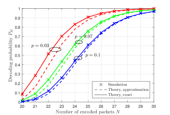
Fig. 2: Performance of the two-destination multicast network as a function $N$, for a fixed $K=20$ and different values of $p$.

We now consider the relay network described in Section III-B. For simplicity, hereafter we assume $N_{R}=N_{S}$. Fig. 3 demonstrates simulated and theoretical values of the decoding probability $P_{R}$ as a function of $N_{S}$, for various values of $K$. The PEP values were selected to describe a typical relay network as follows: $p_{SD}=0.3,p_{SR}=0.1,p_{RD}=0.2$. Fig. 3 also shows the simulated and theoretical performance for a scenario when the relay node is used in the active mode only, as in [11]. It can be seen that the theoretical framework perfectly matches the simulated results. At the same time, the proposed passive relay mode significantly improves the performance, increasing the decoding probability by up to $0.2$. The mode is especially beneficial for high values of $K$, which is explained by a lower influence of the first two terms in (30) when $K$ is increased.

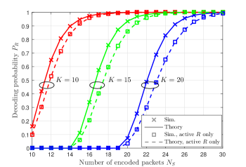
Fig. 3: Performance of the single-relay network as a function of $N_{S}$ for various values of $K$; $p_{SD}=0.3,p_{SR}=0.1$ and $p_{RD}=0.2$.

Fig. 4 illustrates the performance of the relay network as a function of $N_{S}$, but this time for different values of $p_{SD}$ and fixed $K=10$, $p_{SR}=0.1$ and $p_{SR}=0.2$. It is clear in this scenario too that the theoretical results match the simulated ones. At the same time, it can be observed that the effect of the passive relay mode diminishes as the link between the source and destination nodes becomes less reliable. Ultimately, when there is no direct connection between $S$ and $D$ ($p_{SD}=1$), the latter can decode only if $R$ can, hence the passive relay mode becomes redundant.

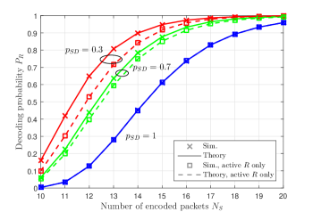
Fig. 4: Performance of the relay network as a function of $N_{S}$ for various values of $p_{SD}$ and fixed $K=10,$ $p_{SR}=0.1$ and $p_{RD}=0.2$.

Finally, the performance of the relay network is investigated for a non-binary code in Fig. 5. Here, we compare codes generated from GF of size $q=2$ and $2^{8}$, for the same value of $K=10$ and $p_{SD}=0.5$, $p_{SR}=0.3$, $p_{RD}=0.4$. It should be noted that such a set of PEP values may describe a random deployment scenario in which none of the links provides a satisfactory performance level. It can be seen that the theoretical framework is valid for the non-binary case as well. As expected, the non-binary code provides a superior performance, offering the same decoding probability as the binary code but requiring fewer encoded packets. The passive relay mode is clearly beneficial for the non-binary code too, improving the decoding probability by up to $0.2$.

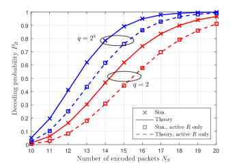
Fig. 5: Performance comparison between codes generated from binary ($q=2$) and non-binary ($q=2^{8}$) codes; $K=10,$ $p_{SD}=0.5$, $p_{SR}=0.3$ and $p_{RD}=0.4$.

V Conclusions

In this work, we investigated the performance of a single-user single-relay network in the context of RLNC, in a scenario where both source and relay nodes encode packets. In contrast with the previous studies related to relay networks, we derived the exact expression for the decoding probability. In the process, we established some fundamental results, such as the probability of two correlated matrices generated from $GF(q)$ being full-rank and the decoding probability of a two-destination multicast network. In addition, we proposed a passive relay mode, in which the relay node re-transmits collected packets if it is not able to decode them. Simulations showed that the established theoretical framework accurately describes the performance of the relay network not only for the binary, but for a non-binary code too. It was also demonstrated that the proposed passive relay mode offers an additional gain in the decoding probability of up to two times, compared with the active-only scenario considered in the previous study. Future work will deal with the generalization of the derived framework to a multiple-relay network.

VI Acknowledgments

This work was performed under the SPHERE IRC funded by the UK Engineering and Physical Sciences Research Council (EPSRC), Grant EP/K031910/1.

References

- [1] R. Ahlswede, N. Cai, S. Y. R. Li, and R. W. Yeung, “Network Information Flow,” IEEE Trans. Inf. Theory, vol. 46, pp. 1204–1216, July 2000.
- [2] M. Médard and A. Sprintson, Network Coding: Fundamentals and Applications. Academic Press, Elsevier, 2012.
- [3] M. Ghaderi, D. Towsley, and J. Kurose, “Reliability Gain of Network Coding in Lossy Wireless Networks,” in Proc. IEEE INFOCOM 2008, (Phoenix, Arizona, US-AZ), pp. 196–200, Apr. 2008.
- [4] A. Tassi, I. Chatzigeorgiou, and D. Vukobratović, “Resource-Allocation Frameworks for Network-Coded Layered Multimedia Multicast Services,” IEEE J. Sel. Areas Commun., vol. 33, pp. 141–155, Feb. 2015.
- [5] X. Li, T. Jiang, Q. Zhang, and L. Wang, “Binary Linear Multicast Network Coding on Acyclic Networks: Principles and Applications in Wireless Communication Networks,” IEEE J. Sel. Areas Commun., vol. 27, pp. 738–748, June 2009.
- [6] R. Gummadi and R. S. Sreenivas, “Relaying a Fountain Code Across Multiple Nodes,” in Proc. of IEEE ITW 2008, (Porto, Portugal, PT), pp. 149–153, May 2008.
- [7] C. F. Chiasserini, E. Viterbo, and C. Casetti, “Decoding Probability in Random Linear Network Coding with Packet Losses,” IEEE Commun. Lett., vol. 17, pp. 1–4, Nov. 2013.
- [8] S. Katti, H. Rahul, W. Hu, D. Katabi, M. Médard, and J. Crowcroft, “XORs in the Air: Practical Wireless Network Coding,” IEEE/ACM Trans. Netw., vol. 16, pp. 497–510, June 2008.
- [9] Y. Qin, F. Yang, X. Tian, X. Wang, H. Luo, H. Wang, and M. Guizani, “Optimal Configuration of Network Coding in Ad Hoc Networks,” IEEE Trans. Veh. Technol., vol. 64, pp. 2001–2014, May 2015.
- [10] X. Fafoutis, E. Tsimbalo, E. Mellios, G. Hilton, R. Piechocki, and I. Craddock, “A Residential Maintenance-Free Long-Term Activity Monitoring System for Healthcare Applications,” EURASIP Journal on Wireless Communications and Networking, vol. 2016, no. 1, pp. 1–20, 2016.
- [11] A. S. Khan and I. Chatzigeorgiou, “Performance Analysis of Random Linear Network Coding in Two-Source Single-Relay Networks,” in Proc. of IEEE ICC 2015, (London, United Kingdom, UK), pp. 991–996, June 2015.
- [12] A. Tassi, C. Khirallah, D. Vukobratović, F. Chiti, J. S. Thompson, and R. Fantacci, “Resource Allocation Strategies for Network-Coded Video Broadcasting Services Over LTE-Advanced,” IEEE Trans. Veh. Technol., vol. 64, pp. 2186–2192, May 2015.
- [13] P. J. S. G. Ferreira, B. Jesus, J. Vieira, and A. J. Pinho, “The Rank of Random Binary Matrices and Distributed Storage Applications,” IEEE Commun. Lett., vol. 17, no. 1, pp. 151–154, 2013.
- [14] A. Papoulis, Probability, Random Variables, and Stochastic Processes. New York: McGraw-Hill, 2nd ed., 1984.