Completeness of general pp-wave spacetimes and their impulsive limit

Abstract.

We investigate geodesic completeness in the full family of pp-wave or Brinkmann spacetimes in their extended as well as in their impulsive form. This class of geometries contains the recently studied gyratonic pp-waves, modelling the exterior field of a spinning beam of null particles, as well as NPWs, which generalise classical pp-waves by allowing for a general wave surface. The problem of geodesic completeness reduces to the question of completeness of trajectories on a Riemannian manifold under an external force field. Building upon respective recent results we derive completeness criteria in terms of the spatial asymptotics of the profile function in the extended case. In the impulsive case we use a fixed point argument to show that irrespective of the behaviour of the profile function all geometries in the class are complete.

PACS class 04.20.Jb, 04.30.-w, 04.30.Nk, 04.30.Db, 02.30.Hq

MSC class 83C15, 83C35, 83C10, 34A36

Keywords: pp-waves, gyratons, geodesic completeness, low regularity, impulsive limit

1. Introduction

Since the seminal work of Penrose [Pen65a] singularities in general relativity are usually understood as the presence of incomplete causal geodesics, i.e., geodesics which cannot be extended to all values of their parameter. In this work we study geodesic completeness for a large class of spacetimes admitting a covariantly constant null vector field, forming the well known pp-wave subclass of the Kundt family of non-twisting, shear-free and non-expanding geometries [Kun61, Kun62]. This subfamily includes, e.g. gyratonic pp-waves [FF05, FZ06], representing the exterior vacuum field of spinning particles moving with the speed of light, which may serve as an interesting toy model in high energy physics [YZF07], but also NP-waves, a generalisation of classical pp-waves allowing for an $n$-dimensional Riemannian manifold $N$ as the wave surface [CFS03]. Remarkably this family of exact spacetimes has already been described by the original Brinkmann form [Bri25] of the pp-wave metric, given in equation (1), below.

We will consider geodesic completeness both in the extended case, i.e., where the profile functions are smooth, as well as in the impulsive case, i.e., when the metric functions are strongly concentrated and of a distributional nature. The problem of completeness in this class of spacetimes can be reduced to a purely Riemannian problem, namely the question of completeness of the motion on a Riemannian manifold under the influence of a time and velocity dependent force. In the extended case we generalise recent results ([CRS12, CRS13]) to the case at hand to provide completeness statements subject to conditions on the spatial fall off of the profile function. We also consider the case of impulsive waves in our class, which are models of short but violent bursts of gravitational radiation emitted by a spinning (beam of) ultrarelativistic particle(s). These models are also interesting from a purely mathematical point of view, since they are examples of geometries of low regularity, which attracted some growing attention recently, see e.g. [CG12, Min15, Sbi15, KSSV15, Säm16]. Our main result here is that all impulsive geometries in the full class of pp-waves are geodesically complete irrespective of the spatial asymptotics of the profile function. This result confirms the effect (previously noted in similar situations, cf. e.g. [PV99, SS12]) that the influence the spatial characteristics of the profile function exert on the behaviour of the geodesics is wiped out in the impulsive limit. In this way we prove a large class of interesting non-smooth geometries to be non-singular in view of the Penrose definition.

This article is structured as follows. In section 2 we introduce the full pp-wave or Brinkmann metric and summarize its basic geometric properties and its algebraic structure. Then, in section 3 we deal with geodesic completeness in the extended case. We review previous works and apply recent results on the completeness of solutions to second order equations on Riemannian manifolds to the geodesic equations for the full Brinkmann metric. In particular, we establish completeness for a large class of physically reasonable (extended) gyratonic pp-waves. In section 4 we introduce impulsive geometries within our general class of pp-wave solutions, thereby leaving the realm of classical smooth Lorentzian geometry. In section 5 we consider the regularised version of these geometries and establish their completeness combining the results of section 3 with a fixed point argument. Finally, in section 6 we explicitly calculate the limits of the complete regularised geodesics given in section 5 and relate them to the geodesics of the background spacetime. Physically this amounts to calculating the geodesics in the distributional model of the impulsive wave.

2. The spacetime metric

In this section we introduce the full pp-wave or Brinkmann metric ([Bri25]) and review some of its basic geometric properties along with relevant subclasses and special cases which have been treated extensively in the literature.

To begin with let $(N,h)$ be a smooth connected $n$-dimensional Riemannian manifold. We consider the spacetime $(M=N\times{\mathbb{R}}^{2},g)$ where the line element is given by

(1) $$ds^{2}=h_{ij}dx^{i}dx^{j}-2dudr+{\mathcal{H}}(x,u)du^{2}+2{\mathcal{A}}_{i}(x,u)dudx^{i}\,.$$

Here ${x=x^{i}=(x^{1},\dots,x^{n})}$ are coordinates on $N$ and $u,r$ are global coordinates on ${\mathbb{R}}^{2}$. Moreover ${\mathcal{H}}:\ N\times{\mathbb{R}}\to{\mathbb{R}}$ and ${\mathcal{A}}_{i}:\ N\times{\mathbb{R}}\to{\mathbb{R}}$ are smooth functions. We fix a time orientation on $M$ by defining the null vector field $\partial_{r}$ to be future directed.

Some immediate geometric properties of the spacetime (1) are the following: $\partial_{r}$ is the generator of the null hypersurfaces of constant $u$, $P(u_{0}):=\{u=u_{0}\}\cong N\times{\mathbb{R}}$, i.e., $\partial_{r}=-\mathrm{grad}u=-\nabla u$ and it is covariantly constant. The latter property is the defining condition for pp-waves (plane fronted waves with parallel rays), and this is why we will refer to (1) as full pp-wave, cf. e.g. [GP09, p. 324 and Sec. 18.5].

The null geodesic generators of $P(u_{0})$ form a non-expanding, shear-free and twist-free congruence and the family of $n$-dimensional spacelike submanifolds $N\times\{u_{0}\}$ orthogonal to $\partial_{r}$ has the interpretation of wave surfaces. Consequently we will also refer to $N$ as the wave surface, and to $h$ and $x^{i}$ as the spatial metric and coordinates, respectively.

Using the coordinates ${(x^{i},u,r)}$ the inverse metric takes the form

(2) $$g^{\mu\nu}=\begin{pmatrix}h^{ij}&0&g^{ri}\\ 0&0&-1\\ g^{ri}&-1&g^{rr}\end{pmatrix}\,,$$

where $h^{ij}$ denotes the components of the inverse spatial metric $h^{-1}$ on $N$, and we have $g^{rr}=-{\mathcal{H}}+h^{ij}{\mathcal{A}}_{i}{\mathcal{A}}_{j}$ and $g^{ri}=h^{ij}{\mathcal{A}}_{j}$. The non-vanishing Christoffel symbols then are

$$\Gamma^{r}_{uu} =g^{ri}({\mathcal{A}}_{i,u}-\tfrac{1}{2}{\mathcal{H}}_{,i})-\tfrac{1}{2}{{\mathcal{H}}_{,u}}\,,$$

(3) $$\Gamma^{r}_{uj} =\tfrac{1}{2}g^{ri}({\mathcal{A}}_{i,j}-{\mathcal{A}}_{j,i})-\tfrac{1}{2}{\mathcal{H}}_{,j}\,,\quad\Gamma^{r}_{jk}=-{\mathcal{A}}_{(j||k)}\,,$$

$$\Gamma^{i}_{uu} =h^{ik}({\mathcal{A}}_{k,u}-\tfrac{1}{2}{\mathcal{H}}_{,k})\,,\quad\Gamma^{i}_{uj}=\tfrac{1}{2}h^{ik}({\mathcal{A}}_{k,j}-{\mathcal{A}}_{j,k})\,,\quad\Gamma^{i}_{jk}={\Gamma^{(N)}}^{i}_{jk}\,,$$

where $\Gamma^{(N)}$ denotes the Christoffel symbols of the Riemannian metric $h$ on $N$, $\,{}_{||}$ stands for the covariant derivative of $h$, and ${\,{}_{,i}}$ and $\,{}_{,u}$ denote derivatives with respect to the $i$-th spatial direction and with respect to $u$, respectively.

From the vanishing of all Christoffel symbols of the form $\Gamma^{u}_{\mu\nu}$ we immediately find that for any geodesic $\gamma(s)=(x^{i}(s),u(s),r(s))$ in (1) we have $\ddot{u}=0$. Hence there are geodesics with $u(s)=u_{0}$ that are entirely contained in the null hypersurface $P(u_{0})$ and thus are either spacelike or the null generators of $P(u_{0})$. Observe that in case ${\mathcal{A}}_{i}=0$, also the $r$-component of these geodesics becomes affine, $r(s)=r_{0}+\dot{r}_{0}s$. All other geodesics may be rescaled to take the form

(4) $$\gamma(s)=(x^{i}(s),s,r(s))\,.$$

The coordinate function $u$ is increasing along any future directed causal curve $c(t)=(x^{i}(t),u(t),r(t))$ since $(u\circ c)\dot{}=g(\nabla u,\dot{c})=\dot{u}\geq 0$ and it is even strictly increasing along any future directed timelike curve. Hence $(M,g)$ is chronological. Moreover $u$ is strictly increasing along all future directed causal geodesics of the form (4). So in case ${\mathcal{A}}_{i}=0$ there is no closed null geodesic segment and the spacetime is even causal.

The non-vanishing components of the Ricci tensor for (1) are

(5) $$R_{ij}=R_{ij}^{(N)}\,,\quad R_{ui}=h^{mn}{\mathcal{A}}_{[m,i]||n}\,,\quad R_{uu}=h^{mn}({\mathcal{A}}_{m,u||n}-\tfrac{1}{2}{\mathcal{H}}_{||mn})+h^{kl}h^{mn}{\mathcal{A}}_{[k,m]}{\mathcal{A}}_{[l,n]}\,,$$

where the square brackets, as usual, denote antisymmetrisation. The Ricci scalar of (1) corresponds to that of the transverse space, i.e., ${R=R^{(N)}}$. Also, the metric (1) belongs to the class of VSI (vanishing scalar invariant) spacetimes iff $N$ is flat.

Next we employ the algebraic Petrov classification ([OPP13, PŠ13]) to the pp-wave metric (1). We project the Weyl tensor onto the natural null frame

(6) $$\mbox{\boldmath$k$}=\mathbf{\partial}_{r}\,,\ \quad\mbox{\boldmath$l$}=\tfrac{1}{2}\,{\mathcal{H}}\,\mathbf{\partial}_{r}+\mathbf{\partial}_{u}\,,\ \quad\mbox{\boldmath$m$}_{(i)}=m_{(i)}^{i}\,({\mathcal{A}}_{i}\,{\partial}_{r}+\mathbf{\partial}_{i})\,,$$

where ${h_{ij}\,m_{(i)}^{i}m_{(j)}^{j}=\delta_{ij}}$ and find that the highest boost weight irreducible components ${\Psi_{0^{ij}}}$, ${\Psi_{1T^{i}}}$ and ${\tilde{\Psi}_{1^{ijk}}}$ vanish and the Brinkmann spacetimes are thus necessarily at least of algebraic type II with ${\mbox{\boldmath$k$}=\mathbf{\partial}_{r}}$ being a double degenerated null direction, in fact ${\Psi_{2^{ij}}=0}$ and (1) is of type II(d). More precisely, without employing any field equations the non-vanishing Weyl scalars are

(7) $$\Psi_{2S} =\tfrac{1}{n(n+1)}\,R^{(N)}\,,$$

(8) $$\tilde{\Psi}_{2T^{(ij)}} =\tfrac{1}{n}\,m_{(i)}^{i}m_{(j)}^{j}\,\big{(}R^{(N)}_{ij}-\tfrac{1}{n}\,h_{ij}\,R^{(N)}\big{)}\,,$$

(9) $$\tilde{\Psi}_{2^{ijkl}} =m_{(i)}^{i}m_{(j)}^{j}m_{(k)}^{k}m_{(l)}^{l}\,C^{(N)}_{ijkl}\,,$$

(10) $$\Psi_{3T^{i}} =\tfrac{1}{n}\,m_{(i)}^{i}\,h^{kl}{\mathcal{A}}_{[i,k]||l}\,,$$

(11) $$\tilde{\Psi}_{3^{ijk}} =m_{(i)}^{i}m_{(j)}^{j}m_{(k)}^{k}\,\Big{(}{\mathcal{A}}_{[k,j]||i}-\tfrac{1}{n-1}\,h^{mn}\,\big{(}h_{ij}{\mathcal{A}}_{[k,m]||n}-h_{ik}{\mathcal{A}}_{[j,m]||n}\big{)}\Big{)}\,,$$

$$\Psi_{4^{ij}} =m_{(i)}^{i}m_{(j)}^{j}\,\Big{(}-\tfrac{1}{2}{\mathcal{H}}_{||ij}+{\mathcal{A}}_{(i,u||j)}+h^{mn}{\mathcal{A}}_{[m,i]}{\mathcal{A}}_{[n,j]}$$

(12) $$\hskip 71.13188pt-\tfrac{1}{n}\,h_{ij}h^{kl}\big{(}-\tfrac{1}{2}{\mathcal{H}}_{||kl}+{\mathcal{A}}_{k,u||l}+h^{mn}{\mathcal{A}}_{[m,k]}{\mathcal{A}}_{[n,l]}\big{)}\Big{)}\,.$$

The boost weight zero components ${\Psi_{2S},\,\tilde{\Psi}_{2T^{(ij)}},\,\tilde{\Psi}_{2^{ijkl}}}$ are entirely governed by the properties of the transverse space $N$, the components of boost weight $-1$, ${\Psi_{3T^{i}}}$, and ${\tilde{\Psi}_{3^{ijk}}}$, are governed by the off-diagonal terms ${\mathcal{A}}_{i}$, while the boost weight $-2$ component ${\Psi_{4^{ij}}}$ depends on all the metric functions ${\mathcal{H}}$ and ${\mathcal{A}}_{i}$. The conditions under which the geometry (1) becomes algebraically more special are summarized in table 1.

Moreover, if the vacuum Einstein field equations (5) are employed some of the conditions are satisfied identically, see table 2.

(sub)type	condition
$\mathrm{II(a)}$	$\displaystyle{R^{(N)}=0}$
$\mathrm{II(b)}$	${R^{(N)}_{ij}=\tfrac{1}{n}\,h_{ij}\,R^{(N)}}$
$\mathrm{II(c)}$	${C^{(N)}_{ijkl}=0}$
$\mathrm{II(d)}$	always
$\mathrm{III}$	$\mathrm{II(abcd)}$
$\mathrm{III(a)}$	${h^{kl}{\mathcal{A}}_{[i,k]||l}=0}$
$\mathrm{III(b)}$	${{\mathcal{A}}_{[k,j]||i}=\tfrac{1}{n-1}\,h^{mn}\,\big{(}h_{ij}{\mathcal{A}}_{[k,m]||n}-h_{ik}{\mathcal{A}}_{[j,m]||n}\big{)}}$
$\mathrm{N}$	$\mathrm{III(ab)}$
$\mathrm{O}$	$-\tfrac{1}{2}{\mathcal{H}}_{||ij}+{\mathcal{A}}_{(i,u||j)}+h^{mn}{\mathcal{A}}_{[m,i]}{\mathcal{A}}_{[n,j]}$
	$=\tfrac{1}{n}\,h_{ij}h^{kl}\big{(}-\tfrac{1}{2}{\mathcal{H}}_{||kl}+{\mathcal{A}}_{k,u||l}+h^{mn}{\mathcal{A}}_{[m,k]}{\mathcal{A}}_{[n,l]}\big{)}$

Table 1. The conditions refining possible algebraic (sub)types of the Brinkmann geometry (1). No field equations are employed. The relations II(b), III(b) are identities for $n=2$ and II(c) for $n=2,3$, respectively. When II(abc) are satisfied simultaneously the transverse space has to be flat.

(sub)type	condition
$\mathrm{II(a)}$	always
$\mathrm{II(b)}$	always
$\mathrm{II(c)}$	${C^{(N)}_{ijkl}=0}$
$\mathrm{II(d)}$	always
$\mathrm{III}$	$\mathrm{II(abcd)}$
$\mathrm{III(a)}$	always
$\mathrm{III(b)}$	${{\mathcal{A}}_{[k,j]||i}=0}$
$\mathrm{N}$	$\mathrm{III(ab)}$
$\mathrm{O}$	$-\tfrac{1}{2}{\mathcal{H}}_{||ij}+{\mathcal{A}}_{(i,u||j)}+h^{mn}{\mathcal{A}}_{[m,i]}{\mathcal{A}}_{[n,j]}=0$

Table 2. The algebraic structure of the spacetimes (1) restricted by Einstein’s vacuum field equations. The algebraic type becomes in general II(abd). Moreover, the condition II(c) is identically satisfied in $n=2,3$ and III(b) in $n=2$, respectively. Condition II(c) necessarily leads to a flat transverse space.

The spacetimes (1) have been originally considered by Brinkmann in the context of conformal mappings of Einstein spaces. Over the decades, starting with Peres [Per59], several special cases of (1) have been used as exact models of spacetimes with gravitational waves.

The most prominent case arises when the wave surface $N$ is flat ${\mathbb{R}}^{2}$ and the off-diagonal terms ${\mathcal{A}}_{i}$ vanish. In fact, writing $x^{i}=(x,y)$ these ‘classical’ pp-waves,

(13) $$ds^{2}=dx^{2}+dy^{2}-2dudr+{\mathcal{H}}(x,y,u)du^{2}\,,$$

have become text book examples of exact gravitational wave spacetimes, see e.g. [GP09, Ch. 17]. The Petrov type is N (cf. table 1) without the application of the field equations hence in any theory of gravity. Moreover, the Ricci tensor simplifies to $R_{uu}=-(1/2)\delta^{ij}{\mathcal{H}}_{,ij}$ (cf. (5)) and its source can be interpreted as any type of null matter or radiation. The vacuum Einstein equations reduce to the $2$-dimensional (flat) Laplacian so that (13) with harmonic ${\mathcal{H}}$ represents pure gravitational waves. Such solutions are most conveniently written using the complex coordinate $\zeta=x+iy$ with ${\mathcal{H}}(\zeta,u)=F(\zeta,u)+F(\bar{\zeta},u)$ and $F$ a combination of terms of the form

(14) $$F(\zeta,u)=\sum_{m=1}^{\infty}\alpha_{m}(u)\,\zeta^{-m}-\mu(u)\log\zeta+\sum_{m=2}^{\infty}\beta_{m}(u)\,\zeta^{m}\,$$

with arbitrary ‘profile functions’ $\alpha_{m}$, $\beta_{m}$, $\mu$ of $u$. Here the inverse-power terms represent pp-waves generated by sources with multipole structure (see e.g. [PG98]) moving along the axis which is clearly singular. Hence it has to be removed from the spacetime which now has spatial part $N={\mathbb{R}}^{2}\setminus\{0\}$. The same is true for the extended Aichelburg–Sexl [AS71] solution represented by the logarithmic term. Finally, the polynomial terms are non-singular with $\beta_{2}$ representing plane waves, see below. The higher order terms ($m\geq 3$) lead to unbounded curvature at infinity and display chaotic behaviour of geodesics (e.g. [PV98]) hence seem to be physically less relevant.

In the special case of ${\mathcal{H}}$ being quadratic in $x,y$ one arrives at plane waves, i.e.,

(15) $$ds^{2}=dx^{2}+dy^{2}-2dudr+{\mathcal{H}}_{ij}(u)x^{i}x^{j}du^{2}\,,$$

where ${\mathcal{H}}_{ij}$ is a real symmetric $(2\times 2)$-matrix-valued function on ${\mathbb{R}}$. Here the curvature tensor components are constant along the wave surfaces and the spacetime is Ricci-flat provided the trace of the profile function vanishes, ${\mathcal{H}}^{i}_{i}=0$, in which case we speak of (purely) gravitational plane waves. While being complete by virtue of the linearity of the geodesic equations, plane waves ‘remarkably’ fail to be globally hyperbolic ([Pen65b]) due to a focussing effect of the null geodesics. This phenomenon has been investigated thoroughly for gravitational plane waves in a series of papers by Ehrlich and Emch ([EE92b, EE92a, EE93], see also [BEE96, Ch. 13]), who were able to determine their precise position on the causal ladder: They are causally continuous but not causally simple. In this analysis, however, the high degree of symmetries of the flat wave surface was extensively used and the ‘stability’ of the respective properties of plane waves within larger classes of solutions remained obscure.

Partly to clarify these matters Flores and Sánchez, in part together with Candela, in a series of papers ([CFS03, FS03, CFS04, FS06]) introduced more general models which they called (general) plane-fronted waves (PFW). Indeed they generalise pp-waves (13) by replacing the flat two-dimensional wave surface by an arbitrary $n$-dimensional Riemannian manifold $N$, i.e., they are defined as (1) with vanishing off-diagonal terms ${\mathcal{A}}_{i}$,

(16) $$ds^{2}=h_{ij}dx^{i}dx^{j}-2dudr+{\mathcal{H}}(x,u)du^{2}\,.$$

Motivated by the geometric interpretation given above and following [SS12] we call these models $N$-fronted waves with parallel rays (NPWs). The Petrov type of these geometries is now II(d) (cf. table 1) and the vacuum field equations become $\Delta_{h}{\mathcal{H}}=h^{ij}{\mathcal{H}}_{||ij}=0$, i.e., the Laplace equation for ${\mathcal{H}}$ on $(N,h)$, which in addition has to be Ricci-flat. Hence vacuum NPWs are necessarily of Petrov type II(abd) and are of type $N$ if and only if $(N,h)$ in addition is conformally flat, hence flat. It turns out that the behaviour of ${\mathcal{H}}$ at spatial infinity is decisive for many of the global properties of NPWs with quadratic behaviour marking the critical case: NPWs are causal but not necessarily distinguishing, they are strongly causal if $-{\mathcal{H}}$ behaves at most quadratically at spatial infinity and they are globally hyperbolic if $-{\mathcal{H}}$ is subquadratic and $N$ is complete. Similarly the global behaviour of geodesics in NPWs is governed by the behaviour of ${\mathcal{H}}$ at spatial infinity. The respective results will be discussed in the next section together with the stronger and newer results of [CRS12, CRS13].

A complementary generalisation of pp-waves (13) was considered by Bonnor ([Bon70]) and independently by Frolov and his collaborators in [FF05, FIZ05, FZ06, YZF07]. Here the $n$-dimensional transverse space $N$ is considered to remain flat but non-trivial off-diagonal terms ${\mathcal{A}}_{i}(x,u)$ are allowed to obtain gyratonic pp-waves

(17) $$ds^{2}=\delta_{ij}dx^{i}dx^{j}-2dudr+{\mathcal{H}}(x,u)du^{2}+2{\mathcal{A}}_{i}(x,u)dudx^{i}\,.$$

Physically this geometry represents a spinning null beam of pure radiation, first called gyraton in [FF05]. By flatness of the wave surface the Petrov type is at least III and in case of vacuum solutions at least III(a) and N if $n=2$ (cf. tables 1, 2). In [Bon70] the metric (17) was matched to an ‘interior’ non-vacuum region, where the spinning source of the gravitational waves was given phenomenologically by an energy momentum tensor of the form $T_{uu}=\rho$ and $T_{ui}=j_{i}$. In the surrounding vacuum region the metric functions ${\mathcal{H}}$ and ${\mathcal{A}}_{i}$ are restricted by the vacuum Einstein equations following from (5) for ${R_{ui}=0}$ and ${R_{uu}=0}$,

(18) $$\delta^{mn}{\mathcal{A}}_{[m,i],n}=0\,,\qquad-\tfrac{1}{2}\,\delta^{mn}{\mathcal{H}}_{,mn}+(\delta^{mn}{\mathcal{A}}_{m,n})_{,u}+\delta^{kl}\delta^{mn}{\mathcal{A}}_{[k,m]}{\mathcal{A}}_{[l,n]}=0\,,$$

where in addition the ‘Lorenz’ gauge ${\delta^{mn}{\mathcal{A}}_{m,n}=0}$ can be applied. In [FF05, FIZ05] explicit solutions have been calculated, all displaying a fall-off like inverse powers of $\|x\|$ if $n>2$ and a logarithmic behaviour if $n=2$. Moreover, the weak field approximation in the presence of a gyratonic source, reflected in the only non-trivial energy-momentum tensor components $T_{uu}$ and $T_{ui}$, gives physical meaning to the metric functions in the entire spacetime. In particular, ${\mathcal{H}}$ determines the mass-energy density and ${\mathcal{A}}_{i}$ correspond to the angular momentum density of the source.

In four dimensions (${n=2}$) the off-diagonal terms in (17) can be removed locally by a coordinate transformation which, however, obscures the global (topological) properties of the spacetime, cf. e.g. [FIZ05, PSŠ14]. In higher dimensions (${n>2}$), the off-diagonal terms in (17) can anyway not be removed even locally due to the lack of coordinate freedom.

The spinning character of four-dimensional gyratonic pp-wave (17) was emphasized in [FIZ05, PSŠ14] employing transverse polar coordinates ${x=\rho\cos\varphi}$, ${y=\rho\sin\varphi}$ with the identifications ${{\mathcal{A}}_{1}=-J\rho^{-1}\sin\varphi}$, ${{\mathcal{A}}_{2}=J\rho^{-1}\cos\varphi}$ which gives

(19) $$ds^{2}=d\rho^{2}+\rho^{2}d\varphi^{2}-2dudr+{\mathcal{H}}(\rho,\varphi,u)du^{2}+2J(\rho,\varphi,u)dud\varphi\,.$$

This can also be understood as the specific form of the full Brinkmann metric (1) with ${x^{1}=\rho}$, ${x^{2}=\varphi}$ and ${dh^{2}=d\rho^{2}+\rho^{2}d\varphi^{2}}$. An important explicit example is given by the axially symmetric gyraton accompanied by a pp-wave generated by a monopole, namely

(20) $$ds^{2}=d\rho^{2}+\rho^{2}d\varphi^{2}-2dudr-2\mu(u)\ln\rho du^{2}+\chi(u)dud\varphi\,,$$

where $\mu(u)$ determines the mass density in the Aichelburg-Sexl-like logarithmic term, and the angular momentum density is determined by $\chi(u)$.

3. Geodesic completeness

In this section we discuss geodesic completeness of the full pp-wave metric (1) and its various special cases in the extended, i.e., smooth case before turning to the impulsive limit in subsequent sections. We will see that all these questions can be reduced to a purely Riemannian question about the completeness of trajectories on $N$ under a specific force field.

The explicit form of the system of geodesic equations for a curve $\gamma(s)=(x^{i}(s),u(s),r(s))$ is, see (3),

(21) $$\ddot{x}^{i} =-{\Gamma^{(N)}}^{i}_{jk}\,\dot{x}^{j}\dot{x}^{k}-h^{ik}({\mathcal{A}}_{k,j}-{\mathcal{A}}_{j,k})\,\dot{x}^{j}\dot{u}-\tfrac{1}{2}h^{ik}(2{\mathcal{A}}_{k,u}-{\mathcal{H}}_{,k})\,\dot{u}^{2}\,,$$

(22) $$\ddot{u} =0\,,$$

(23) $$\ddot{r} ={\mathcal{A}}_{(i||j)}\,\dot{x}^{i}\dot{x}^{j}-\Big{(}g^{ri}({\mathcal{A}}_{i,j}-{\mathcal{A}}_{j,i})-{\mathcal{H}}_{,j}\Big{)}\,\dot{u}\dot{x}^{j}-\Big{(}g^{ri}({\mathcal{A}}_{i,u}-\tfrac{1}{2}{\mathcal{H}}_{,i})-\tfrac{1}{2}{\mathcal{H}}_{,u}\Big{)}\,\dot{u}^{2}\,.$$

We observe (again) that the equation for $u$ is trivial and that the equation for $r$ decouples from the rest of the system and can simply be integrated once the $x$-equations are solved. Finally the $x$-equations are the equations of motion on the Riemannian manifold $N$ under an external force term depending on time and velocity. Hence the basic result on the form of the geodesics of the Brinkmann metric (1) is the following (cf. [CFS03, Prop. 3.1]):

Proposition 3.1 (Form of the geodesics).

Let $\gamma=(x^{i},u,r):\,(-a,a)\to M$ be a curve on $M$ with constant ‘energy’ $E_{\gamma}=g(\dot{\gamma},\dot{\gamma})$ which assumes the data

(24) $$\gamma(0)=(x^{i}_{0},u_{0},r_{0})\,,\quad\dot{\gamma}(0)=(\dot{x}^{i}_{0},\dot{u}_{0},\dot{r}_{0})\,.$$

Then $\gamma$ is a geodesic iff the following conditions hold true

1. $u$ is affine, i.e., $u(s)=u_{0}+s\dot{u}_{0}$ for all $s\in(-a,a)$,

2. $x^{i}$ solves

   (25) $$D_{\dot{x}}\dot{x}^{i}=-h^{ik}({\mathcal{A}}_{k,j}-{\mathcal{A}}_{j,k})\,\dot{x}^{j}\dot{u}_{0}-\tfrac{1}{2}h^{ik}(2{\mathcal{A}}_{k,u}-{\mathcal{H}}_{,k})\dot{u}_{0}^{2}\,,$$

   where $D$ denotes the covariant derivative of $(N,h)$,

3. $r$ is given by

   $$r(s)= \,r_{0}$$

   (26) $$-\frac{1}{2\dot{u}_{0}}\int\limits_{0}^{s}\left(E_{\gamma}-h(\dot{x}(\sigma),\dot{x}(\sigma))-\dot{u}_{0}^{2}H(x(\sigma),u(\sigma))-2\dot{u}_{0}{\mathcal{A}}_{i}(x(\sigma),u(\sigma))\dot{x}^{i}(\sigma)\right){\rm d}\sigma\,.$$

Here we have used the explicit form of $E_{\gamma}$ in the last condition. The key fact is now that completeness essentially depends on completeness of the solutions to (25). Note that in most cases we will use a rescaling to achieve the form (4) of the geodesics, which amounts to setting $u_{0}=0$ and $\dot{u}_{0}=1$ in equations (25) and ((c)).

Corollary 3.2 (Basic condition for completeness).

The spacetime (1) is complete iff all inextendible solutions of (25) are complete.

Although there are some results also in case of an incomplete spatial manifold, see the discussion after Corollary 3.4 below, we assume for the moment $(N,h)$ to be complete. The question of completeness of solutions of equations as (25) has, if only in special cases, been addressed in the ‘classical’ literature. To begin with, we observe that in the special case of NPWs (16) the equation of motion (25) reduces to

(27) $$D_{\dot{x}}\dot{x}=\frac{1}{2}\nabla_{x}{\mathcal{H}}(x,s)\,$$

($\nabla_{x}$ denoting the gradient on $(N,h)$), i.e., to the equation of motion on $N$ under the influence of a time dependent potential. First results on the completeness of NPWs, mainly restricted to the case of autonomous ${\mathcal{H}}$, i.e., ${\mathcal{H}}={\mathcal{H}}(x)$ independent of $u$ were derived in [CFS03, Sec. 3]. In fact, it follows from e.g. [AM78, Thm. 3.7.15] that a NPW (16) is complete if ${\mathcal{H}}$ is autonomous and controlled by a positively complete function at infinity, i.e., if there exists some arbitrarily fixed $\bar{x}\in N$ and some positive constant $\mathfrak{R}$ such that

(28) $${\mathcal{H}}={\mathcal{H}}(x)\leq-V(d(x,\bar{x}))\quad\text{for all $x\in N$ with $d(x,\bar{x})\geq\mathfrak{R}$}\,,$$

where $d$ denotes the Riemannian distance function on $(N,h)$ and $V:\,[0,\infty)\to{\mathbb{R}}$ is $C^{2}$ with $\int_{0}^{\infty}dx/\sqrt{e-V(x)}=+\infty$ for one (hence any) $e>V(x)$ and all $x$. Consequently autonomous NPW are complete if ${\mathcal{H}}$ grows at most quadratically at spatial infinity, i.e, if $\exists\ \bar{x}\in N,\ \mathfrak{R}>0$ such that

(29) $${\mathcal{H}}={\mathcal{H}}(x)\leq C\,d^{2}(x,\bar{x})\quad\text{for all $x$ with $d(x,\bar{x})\geq\mathfrak{R}$}\,,$$

for some constant $C>0$. Of course this result extends immediately to sandwich NPWs, which grow at most quadratically at spatial infinity. Also the case of plane NPWs is easily settled, that is (16) with $(N,h)$ flat and quadratic non-autonomous ${\mathcal{H}}$, i.e.,

(30) $${\mathcal{H}}(x,u)=h(A(u)x,x)\,,$$

where $A$ is (at least) a continuous map from ${\mathbb{R}}$ into the space of real symmetric $(n\times n)$-matrices. Here completeness follows from global existence of solutions to linear ODEs generalising the case of plane waves (15).

More substantial results on non-autonomous NPWs have been given in [CRS12] based on recent results on the completeness of trajectories of equations like (25) and (27) in [CRS13]. (For more general and somewhat sharper results see [Min15].) Since we will use these statements also in our discussion of the general case (1) we recall in the following the key notions and theorems. We say that a (time dependent) tensor field $X$ on the projection $\pi:N\times{\mathbb{R}}\to N$ grows at most linearly in $N$ along finite times if for all $T>0$ there exists $\bar{x}\in N$ and constants $A_{T},C_{T}>0$ such that

(31) $$|X|_{(x,s)}\leq A_{T}\,d(x,\bar{x})+C_{T}\quad\forall(x,s)\in N\times[-T,T]$$

with $|\ |$ and $d$ the norm and the distance function of $h$, respectively. Analogously we define the notions of at most quadratic growth along finite times and boundedness along finite times, where in the special case of functions we use the estimate (31) without norm. Now given a smooth $(1,1)$-tensor field $F$ and a smooth vector field $X$ on $\pi$ we consider the second order ODE

(32) $$D_{\dot{\gamma}}\dot{\gamma}(s) =F_{(\gamma(s),s)}\dot{\gamma}(s)+X_{(\gamma(s),s)}\,$$

and the special case when $X$ is derived from a potential, i.e.,

(33) $$D_{\dot{\gamma}}\dot{\gamma}(s) =F_{(\gamma(s),s)}\dot{\gamma}(s)-\nabla_{x}V{(\gamma(s),s)}\,$$

with $V$ a smooth function on $N\times{\mathbb{R}}$. Then we have

Theorem 3.3 (Theorems 1,2 in [CRS13]).

Let $(N,h)$ be a connected, complete Riemannian manifold. If the self adjoint part $S$ of $F$ is bounded in $N$ along finite times then

1. all inextendible solutions of (32) are complete provided $X$ grows at most linearly in $N$ along finite times, and

2. all inextendible solutions of (33) are complete provided that $-V$ and $|\frac{\partial V}{\partial s}|$ grow at most quadratically in $N$ along finite times.

Observe that one may also apply Theorem 3.3(1) to equation (33) in which case one has to assume that $\nabla_{x}V$ grows at most linearly along finite times. Provided that we are in the non-autonomous case this condition is logically independent of the condition of Theorem 3.3(2).

Hence in the case of NPWs, which amounts to setting $F=0$ and $X=-\nabla_{x}V=\nabla_{x}{\mathcal{H}}$, one obtains different types of results based on either of these conditions, see [CRS12, CRS13]. Explicitly we have

Corollary 3.4 (Completeness of NPWs and classical pp-waves).

NPW spacetimes (16) and, in particular, classical pp-wave spacetimes (13) with complete wave surface $N$ are complete provided that either

1. $\nabla_{x}{\mathcal{H}}$ grows at most linearly along finite times, or

2. ${\mathcal{H}}$ and $\left|\frac{\partial{\mathcal{H}}}{\partial s}\right|$ grow at most quadratically along finite times, or

3. ${\mathcal{H}}(x,u)\leq\beta_{0}(u)$ and $\left|\frac{\partial{\mathcal{H}}}{\partial u}(x,u)\right|\leq\alpha_{0}(u)\big{(}\beta_{0}(u)-{\mathcal{H}}(x,u)\big{)}$ for some continuous real functions $\alpha_{0}$, $\beta_{0}$ and all $(x,u)\in N\times{\mathbb{R}}$.

Condition (3) is, however, not derived from Theorem 3.3 but due to [CRS12, Cor. 3.3] and again logically independent of the other conditions. A physically interesting consequence of condition (2), which actually generalises the above results on autonomous and sandwich NPWs of quadratic growth, is that it provides stability of completeness of plane waves within the class of NPWs with quadratic behaviour of ${\mathcal{H}}$, cf. [CRS12, Rem. 3.5].

Observe that physically reasonable models of classical gravitational pp-waves, as discussed below equation (14), possess a non-complete wave surface and hence Corollary 3.4 does not apply in this case. However, the geodesics will still be ‘complete at infinity’ since the asymptotic conditions of Corollary 3.4 hold true for the multipole as well as for the logarithmic terms in (14). However, the geodesics could leave the exterior region ‘at the inside’ proceeding to the matter region. This behaviour clearly has to be considered as physically reasonable. Also mathematically completeness of trajectories of (32), (33) on incomplete Riemannian manifolds is subject to very strong conditions, see e.g. [Gor70]: A sufficient condition, e.g. is that ${\mathcal{H}}$ is proper and bounded from below, which certainly does not hold in our case. Note that this applies to wave surfaces of the form $N={\mathbb{R}}^{n}\setminus\{0\}$ as well as to those of the form ${\mathbb{R}}^{n}$ with a (closed) ball removed. In the latter case one would of course match the solution to some non-vacuum interior region inside the ball. The situation is of course completely analogous in case of NPWs.

Turning now to the general case, i.e., to the quest for completeness of the full pp-wave geometry (1) we more extensively make use of the power of Theorem 3.3. Indeed $F^{i}_{j}=-h^{ik}({\mathcal{A}}_{k,j}-{\mathcal{A}}_{j,k})$ is no longer vanishing but still its selfadjoint part satisfies $S=0$ so that Theorem 3.3 puts no restriction on ${\mathcal{A}}_{k,j}$. On the other hand, $X=-\frac{1}{2}h^{ik}(2{\mathcal{A}}_{k,u}-{\mathcal{H}}_{,k})$ and we can no longer write $X$ as the gradient of a potential. So we cannot use condition (2) and have to exclusively resort to Theorem 3.3(1). In this way we obtain

Corollary 3.5 (Completeness of the Brinkmann metric).

The full pp-wave spacetime (1) is complete if $N$ is complete and $\nabla_{x}{\mathcal{H}}$ and $h^{ik}{\mathcal{A}}_{k,u}$ grow at most linearly along finite times.

Finally, we come to discuss completeness of gyratonic pp-waves (17). In this case the wave surface is flat and so we only have to deal with the asymptotics of the metric functions.

Corollary 3.6 (Completeness of gyratons).

Any gyratonic pp-wave (17) with $N={\mathbb{R}}^{n}$ and ${\mathcal{H}}_{,x}$ as well as ${\mathcal{A}}_{k,u}$ growing at most linearly along finite times is complete.

Now the asymptotics of the explicit gyratonic pp-waves of [FF05, FIZ05], see section 2, p. 18 imply that ${\mathcal{H}}_{,k}$ and ${\mathcal{A}}_{k,u}$ even decay or only grow logarithmically for large $x$. However, again physically reasonable models are singular on the axis (cf. e.g. (20)) or should be matched to some interior matter region so that the wave surface is ${\mathbb{R}}^{n}$ without a point or ${\mathbb{R}}^{n}$ with a ball removed and hence incomplete. So again we obtain for such ‘gravitational’ gyratons only ’completeness at infinity’ but the geodesics could leave the exterior region ‘at the inside’ proceeding into the matter region. This behaviour again is to be considered as physically perfectly reasonable.

4. Impulsive limit

In this section we turn our focus to impulsive versions of the Brinkmann metric (1). Generally, impulsive gravitational waves model short but violent pulses of gravitational or other radiation. In particular, in his seminal work [Pen72], R. Penrose has considered impulsive pp-waves, that is spacetimes of the form (13) with

(34) $${\mathcal{H}}(x,u)=H(x)\delta(u)\,,$$

where $\delta$ denotes the Dirac function and $H$ is a function of the spatial variables only. Since then various methods of constructing impulsive gravitational waves with or without cosmological constant have been introduced, for an overview see e.g. [GP09, Ch. 20]. In particular, impulsive gravitational waves have been found to arise as ultrarelativistic limits of Kerr-Newman and other static spacetimes which make them interesting models for quantum scattering in general relativistic spacetimes.

More generally, impulsive NPWs (iNPWs), i.e., (16) with (34) have been considered in [SS12, SS15]. In all these models, which are impulsive versions of special cases of (1) with the off-diagonal terms ${\mathcal{A}}_{i}$ vanishing, the field equations put no restriction on the $u$-behaviour of the profile function ${\mathcal{H}}$, see Section 2. Hence the most straightforward approach to impulsive waves in this class of solutions indeed is to view them as impulsive limits of sandwich waves with ever shorter but stronger profile function which precisely leads to (34).

Here we are, however, mainly interested in impulsive versions of the full pp-wave spacetimes (1), which in particular includes impulsive versions of gyratonic pp-waves (17). Here the situation is more subtle as detailed in [FF05, FIZ05], where such geometries have been considered along with their extended versions. A more detailed discussion of four-dimensional geometries with a flat transverse space in the form (19) was given recently in [PSŠ14, Sec. 7]. Since this discussion also applies to the general case and leads to our model of the impulsive full pp-wave metric we briefly recall it here. To begin with we introduce the convenient quantity

(35) $$\omega(\rho,\varphi,u)\equiv\frac{J_{,\rho}(\rho,\varphi,u)}{2\rho}\,,$$

such that the vacuum field equations take the form (with $\triangle$ denoting the flat Laplacian)

(36) $$\omega_{,\varphi}=0\,,\qquad\omega_{,\rho}=0\,,\qquad\triangle\,{\mathcal{H}}=4\,\omega^{2}+\frac{2}{\rho^{2}}\,J_{,u\varphi}\,,$$

implying ${\omega=\omega(u)}$ which corresponds to a rigid rotation. Relation (35) immediately gives

(37) $$J=\omega(u)\,\rho^{2}+\chi(u,\varphi)\,,$$

where ${\chi(u,\varphi)}$ is an arbitrary $2\pi$-periodic function in $\varphi$. Taking (37) and a suitable ansatz for ${\mathcal{H}}$,

(38) $${\mathcal{H}}=\omega^{2}(u)\,\rho^{2}+2\,\omega(u)\,\chi(u,\varphi)+{\mathcal{H}}_{0}(u,\rho,\varphi)\,,$$

the remaining field equation in (36) becomes

(39) $$\triangle\,{\mathcal{H}}_{0}=\rho^{-2}\,\Sigma\,,\qquad\hbox{with}\qquad\Sigma(u,\varphi)\equiv 2(\chi_{,u\varphi}-\omega\,\chi_{,\varphi\varphi})\,.$$

Removing the rigid rotation by the the natural global gauge ${\omega=0}$, and using the splitting

(40) $${\mathcal{H}}_{0}(u,\rho,\varphi)=\tilde{\mathcal{H}}_{0}(\rho,\varphi)\,\chi_{H}(u)\,,\qquad\chi(u,\varphi)=\tilde{\chi}(\varphi)\,\chi_{J}(u)+\Phi(\varphi)\,,$$

we obtain ${\Sigma(u,\varphi)=2\tilde{\chi}_{,\varphi}(\varphi)\,{\chi_{J}}_{,u}(u)}$ and equation (39) takes the form

(41) $$\triangle\tilde{\mathcal{H}}_{0}(\rho,\varphi)\,\chi_{H}(u)=\frac{2}{\rho^{2}}\ \tilde{\chi}_{,\varphi}(\varphi)\,{\chi_{J}}_{,u}(u)\,.$$

If ${\Sigma=0}$, i.e., ${\tilde{\chi}(\varphi)=const.}$, equation (41) reduces to ${\triangle\,{\mathcal{H}}_{0}=0}$ and there is no restriction on the $u$-dependence of ${\mathcal{H}}_{0}$ and $J$. In particular, the energy profile $\chi_{H}(u)$ and the angular momentum density profile $\chi_{J}(u)$ can be taken independently of each other. In [PSŠ14] it was demonstrated that the curvature is proportional to $\chi_{H}$ and ${\chi_{J}}_{,u}$ which leads to impulsive waves by setting $\chi_{H}(u)$ to be proportional to the Dirac $\delta$ but using a box-like profile for $\chi_{J}(u)$.

However, in the case when $\Sigma\not=0$ there occurs a coupling of the profile functions. Indeed the supports of $\chi_{H}(u)$ and ${\chi_{J}}_{,u}(u)$ have to coincide since otherwise both sides of (41) have to vanish individually, leading to the vanishing of $\tilde{\chi}_{,\varphi}(\varphi)$ and hence $\Sigma$. In particular, the box profile in the angular momentum density $\chi_{J}(u)$ leads to two Dirac deltas in the energy density.

Moreover, we can of course combine such a coupled solution with specific homogeneous solutions. Hence it is most natural and physically relevant to prescribe a general box-like profile for the angular momentum density and a delta-like profile for the energy density of the form

(42) $${\mathcal{H}}(x,u)=H(x)\delta_{\alpha,\beta}(u)\,,\quad{\mathcal{A}}_{i}(x,u)=a_{i}(x)\vartheta_{L}(u)\,,$$

where we define (see Figure 1, below)

(43) $$\delta_{\alpha,\beta}(u)=\alpha\delta(u)+\beta\delta(u-L),\quad\text{and}\quad\vartheta_{L}(u)=\frac{1}{L}\big{(}\Theta(u)-\Theta(u-L)\big{)}\,.$$

Here $\alpha$, $\beta$, and $L>0$ are some constants, $\delta$ denotes the Dirac measure and $\Theta$ is the Heaviside function. This ansatz covers the coupled case ($\alpha=1/L,\beta=-1/L$) as well as all the models studied in [YZF07] ($p$-gyraton: $\alpha=0=\beta$, AS-gyraton: $a_{i}=0=\beta$, $a$-gyraton: $\alpha>0$, $\beta=0$, $b$-gyraton: $\alpha=0$, $\beta>0$), which all arise from specific combinations of homogeneous solutions.

So the impulsive full pp-wave metric we will consider in the rest of our work is explicitly given by

(44) $$ds^{2}=h_{ij}dx^{i}dx^{j}-2dudr+H(x)\delta_{\alpha,\beta}(u)du^{2}+2a_{i}(x)\vartheta_{L}(u)dudx^{i}\,.$$

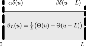
Figure 1. Illustration of the box-like profile with accompanying delta-spikes.

Of course, off the wave zone (given by $u\in[0,L]$) the spacetime is just the product of the Riemannian wave surface $(N,h)$ with flat ${\mathbb{R}}^{2}$. From now on we will assume $(N,h)$ to be complete and call $M_{0}=N\times{\mathbb{R}}^{2}$ the background of the impulsive wave (44), which is then complete as well. From (7)–(12) we immediately observe that the components of boost weight ${-1}$ and of ${-2}$, namely,

(45) $$\Psi_{3T^{i}} =\tfrac{1}{n}\,m_{(i)}^{i}\,h^{kl}a_{[i,k]||l}\,\vartheta_{L}\,,$$

(46) $$\tilde{\Psi}_{3^{ijk}} =m_{(i)}^{i}m_{(j)}^{j}m_{(k)}^{k}\,\Big{(}a_{[k,j]||i}-\tfrac{1}{n-1}\,h^{mn}\,\big{(}h_{ij}a_{[k,m]||n}-h_{ik}a_{[j,m]||n}\big{)}\Big{)}\,\vartheta_{L}\,,$$

$$\Psi_{4^{ij}} =m_{(i)}^{i}m_{(j)}^{j}\,\Big{(}-\tfrac{1}{2}H_{||ij}\,\delta_{\alpha,\beta}+a_{(i||j)}\,\delta_{L^{-1},-L^{-1}}+h^{mn}a_{[m,i]}a_{[n,j]}\,{\vartheta_{L}}^{2}$$

(47) $$\hskip 71.13188pt-\tfrac{1}{n}\,h_{ij}h^{kl}\big{(}-\tfrac{1}{2}H_{||kl}\,\delta_{\alpha,\beta}+a_{k||l}\,\delta_{L^{-1},-L^{-1}}+h^{mn}a_{[m,k]}a_{[n,l]}\,{\vartheta_{L}}^{2}\big{)}\Big{)}\,,$$

are only non-trivial in the wave zone while, in general, the rest of the spacetime corresponds to the type D background.

5. Completeness of the impulsive limit

We first review previous results on the completeness of impulsive gravitational waves. In the simplest case of classical impulsive pp-waves, i.e., (13) with (34), the spacetime is flat Minkowski space off the single wave surface $\{u=0\}$ where the curvature is concentrated. Consequently, the geodesics for impulsive pp-waves have been derived in the physics literature (see e.g. [FPV88]) by matching the geodesics of the background on either side of the wave in a heuristic manner—the geodesic equation contains nonlinear terms, ill-defined in distribution theory. This approach, in particular, leaves it open whether the geodesics cross the wave surface at all.

In [KS99a, KS99b] this question has been answered in the affirmative using a regularisation approach within the theory of nonlinear distributional geometry ([GKOS01, Ch. 4]) based on algebras of generalized functions ([Col85]). In this way a completeness result for all impulsive pp-waves, i.e., for all smooth profile functions $H$, was achieved although this aspect was not emphasised in the original works. Observe that this contrasts the completeness results in the extended case (Corollary 3.4) where the spatial asymptotics of ${\mathcal{H}}$ enters decisively. Moreover this approach in a limiting process establishes that the geodesics in the entire spacetime are indeed the straight line geodesics of the background which are refracted by the impulse to become broken and possibly discontinuous.

More generally in [SS12, SS15] geodesics in iNPWs, i.e., (16) with (34), were investigated. Again using a regularisation approach it was proven that if the wave surface $N$ is complete, then the iNPW is geodesically complete irrespective of the behaviour of the profile function $H$. Again this is in contrast to the extended case where the completeness depends crucially on the spatial asymptotic behaviour of the profile function ${\mathcal{H}}$, see Section  3. Moreover, the geodesics in the limit again are geodesics of the background, which are refracted by the impulse, see also [FIZ05] for a heuristic argument. More precisely, using a fixed point argument it was shown in [SS12] that in the regularised iNPW

(48) $$ds_{\varepsilon}^{2}=h_{ij}dx^{i}dx^{j}-2dudr+\delta_{\varepsilon}(u)H(x)du^{2}\,,$$

with $\delta_{\varepsilon}$ a standard mollifier, geodesics are complete in the following sense: For each point $p\in M$ ‘in front’ of the impulsive wave, i.e., $u<0$ and each tangent direction $v\in T_{p}M$ we consider the geodesic $\gamma_{\varepsilon}$ of (48) starting in $p$ into direction $v$. If $\gamma_{\varepsilon}$ reaches the regularised wave zone given by $\{|u|\leq\varepsilon\}$ then there is an $\epsilon_{0}>0$ such that for all $0<\epsilon\leq\epsilon_{0}$ the geodesic $\gamma_{\varepsilon}$ passes through the regularised wave zone and continues as (complete) geodesic of the background ‘behind’ the impulsive wave. This result has been rephrased in the language of nonlinear distributional geometry in [SS15], which allows to omit the reference to the initial data in the final completeness statement.

As is well known, classical impulsive pp-waves and more generally non-expanding as well as expanding impulsive gravitational waves propagating in constant curvature backgrounds have also been described by a continuous form of the metric, see e.g. [GP09, Ch. 20]. Actually these metrics are locally Lipschitz continuous and hence the geodesics equations possess locally bounded but possibly discontinuous right hand sides. Employing the solution concepts of Carathéodory and Filippov ([Fil88]), respectively, these systems of ODEs have been recently investigated leading to the following results: The geodesics are complete and of $C^{1}$-regularity in classical pp-waves ([LSŠ14]), non-expanding ([PSSŠ15]) and expanding ([PSSŠ16]) impulsive waves propagating on Minkowski, de Sitter, and anti-de Sitter backgrounds. However, so far no continuous form of the impulsive full pp-wave metric or merely of the gyratonic pp-wave metric has been found.

Geodesic completeness for non-expanding impulsive gravitational waves in (anti-)de Sitter space has also been proven in the distributional picture in [SSLP16] using a regularisation approach and a fixed point argument in a spirit similar to the present article. Finally a proof of geodesic completeness of impulsive gyratonic pp-waves has been sketched in [PSŠ14, Section VIII].

In the following we provide our main result which establishes completeness of the impulsive full pp-wave metric (44) using a regularisation approach.

To begin with we consider the regularised metric

(49) $$ds^{2}_{\varepsilon}=h_{ij}dx^{i}dx^{j}-2dudr+H(x)\delta^{\varepsilon}_{\alpha,\beta}(u)du^{2}+2a_{i}(x)\vartheta^{\varepsilon}_{L}(u)dudx^{i}\,,$$

where we have regularised the profile functions replacing $\delta$ by a standard mollifier

(50) $$\delta_{\varepsilon}(x)=\frac{1}{\varepsilon}\,\phi\left(\frac{x}{\varepsilon}\right)$$

with $\phi$ a smooth function supported in $[-1,1]$ with unit integral. Moreover we have regularised the Heaviside function by the primitive of $\delta_{\varepsilon}$, i.e., replacing $\Theta$ by

(51) $$\Theta_{\epsilon}(x)\equiv\int_{-1}^{x}\delta_{\epsilon}(t)\,{\rm d}t.$$

More explicitly we set

(52) $$\delta^{\varepsilon}_{\alpha,\beta}(u)=\alpha\delta_{\varepsilon}(u)+\beta\delta_{\varepsilon}(u-L)\,,\quad\text{and}\quad\vartheta^{\varepsilon}_{L}(u)=\frac{1}{L}\big{(}\Theta_{\varepsilon}(u)-\Theta_{\varepsilon}(u-L)\big{)}\,.$$

In the following we will prove that any geodesic in the regularised impulsive full pp-wave metric (49) that reaches the wave zone given by ${\{u\in[-\varepsilon,L+\varepsilon]\}}$ will pass through it, provided that $\varepsilon$ is small enough. This will lead to our main result on the completeness of the impulsive full pp-wave metric (44) which we state at the end of this section. In the final section 6 we will relate these complete geodesics to the geodesics of the background.

To begin with we give the explicit form of the geodesic equations for the metric (49). Observe that also in the present case the $u$-equation is trivial and hence we may use a rescaling as in (4) to write any geodesic not parallel to, or contained in the impulsive wave surface $\{u=0\}$ as

(53) $$\gamma_{\varepsilon}(s)=(x^{i}_{\varepsilon}(s),s,r_{\varepsilon}(s)).$$

Now we obtain, cf. (21)

$$\ddot{r}_{\varepsilon} =\vartheta^{\varepsilon}_{L}\,a_{(i||j)}\,\dot{x}^{i}_{\varepsilon}\dot{x}^{j}_{\varepsilon}-\Big{(}g_{\varepsilon}^{ri}\vartheta^{\varepsilon}_{L}\,\big{(}a_{i,j}-a_{j,i}\big{)}-H_{,j}\,\delta^{\varepsilon}_{\alpha,\beta}\Big{)}\,\dot{x}^{j}_{\varepsilon}$$

(54) $$\qquad\quad-\Big{(}g_{\varepsilon}^{ri}\big{(}a_{i}\,\delta^{\varepsilon}_{L^{-1},-L^{-1}}-\tfrac{1}{2}H_{,i}\,\delta^{\varepsilon}_{\alpha,\beta}\big{)}-\tfrac{1}{2}H\,(\delta^{\varepsilon}_{\alpha,\beta})_{,u}\Big{)}\,,$$

(55) $$\ddot{x}_{\varepsilon}^{i} =-{\Gamma^{(N)}}^{i}_{jk}\,\dot{x}_{\varepsilon}^{j}\dot{x}_{\varepsilon}^{k}-\vartheta^{\varepsilon}_{L}\,h^{ik}\big{(}a_{k,j}-a_{j,k}\big{)}\,\dot{x}^{j}-\tfrac{1}{2}h^{ik}\big{(}2a_{k}\,\delta^{\varepsilon}_{L^{-1},-L^{-1}}-H_{,k}\,\delta^{\varepsilon}_{\alpha,\beta}\big{)}\,,$$

where $g_{\varepsilon}^{ri}=h^{ik}a_{k}\,\vartheta_{L}^{\varepsilon}$.

As in the extended case the $r$-equation can simply be integrated once the $x$-equations are solved and completeness of the geodesics is determined by completeness of the solutions to the spatial equations, cf. Proposition 3.1. The latter again take the form of the equations of motion on the Riemannian manifold $(N,h)$, now with an external force term depending on time, velocity and the regularisation parameter $\varepsilon$. More explicitly we may rewrite equation (55) in the form, cf. (32)

(56) $$D_{\dot{x}_{\varepsilon}}\dot{x}_{\varepsilon}(s)=F^{\varepsilon}_{(x_{\varepsilon}(s),s)}\dot{x}_{\varepsilon}(s)+X^{\varepsilon}_{(x_{\varepsilon}(s),s)}\ ,$$

where $D$ denotes the connection on $(N,h)$ and we have set $F^{i\,\varepsilon}_{j}=-\vartheta^{\varepsilon}_{L}\,h^{ik}(a_{k,j}-a_{j,k})$ and $X^{i\,\varepsilon}=-\tfrac{1}{2}h^{ik}\big{(}2a_{k}\,\delta^{\varepsilon}_{L^{-1},-L^{-1}}-H_{,k}\,\delta^{\varepsilon}_{\alpha,\beta}\big{)}$.

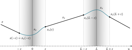
Figure 2. An illustration of the construction leading to Theorem 5.3. The $x$-component of the seed geodesic $\gamma$ is drawn in bold black and the regularised geodesic given by Proposition 5.1 are drawn dotted in blue. The seed geodesic provides the initial data for the geodesic $x_{\varepsilon}$ at $-\varepsilon$ which on $[-\varepsilon,\varepsilon]$ solves (55) and continues as a solution of (71) until $L-\varepsilon$, where it provides new initial data for a solution $x_{\varepsilon}$ of (55) until $L+\varepsilon$ and then continues as a solution of the background geodesic equation (66) with data (75).

Now for fixed $\varepsilon$ the solutions will be complete by Corollary 3.5 provided $H$ and $a_{i}$ show a suitable asymptotic behaviour. But here we aim at a result for general $H$ and $a_{i}$ and so we have to take a different approach. Indeed, for fixed $\varepsilon$ by ODE-theory we have a local solution $x_{\varepsilon}$ for any initial condition taken at the say ‘left’ boundary of the wave zone $u=-\varepsilon$, see Figure 2. However, the time of existence of such a solution will in general depend upon the regularisation parameter $\varepsilon$ and could shrink to zero if $\varepsilon\to 0$. We will prove that this is not the case. More precisely, applying a fixed point argument we will show that such solutions $x_{\varepsilon}$ have a uniform (in $\varepsilon$) lower bound $\eta$ on their time of existence, which will at least for small $\varepsilon$ allow them to cross the regularisation region of the first $\delta$-spike, i.e., $|u|\leq\varepsilon$. Once they reach $u=\varepsilon$ they are subject to equations (55) with only the $\vartheta^{\varepsilon}$-terms being non-trivial. In other words we have to deal with (56) with $X^{\varepsilon}$ vanishing. In this situation we may now apply the completeness results established in Section 3. More precisely, we appeal to Theorem 3.3(1) whose assumptions hold anyway in our case and we obtain that the solution $x_{\varepsilon}$ will continue at least until it reaches the regularisation region of the second $\delta$-spike at $u=L-\varepsilon$. There we can, however, reapply our fixed point argument to secure that $x_{\varepsilon}$ reaches $u=L+\varepsilon$ and hence leaves the entire wave zone to enter the background region ‘behind’ the wave.

We will now state and prove the fixed point argument. To simplify notations we will, instead of dealing with equation (55) directly, consider the following model initial value problem

(57) $$\ddot{x}_{\varepsilon} =F_{1}(x_{\varepsilon},\dot{x}_{\varepsilon})+F_{2}(x_{\varepsilon})\delta_{\varepsilon}+F_{3}(x_{\varepsilon},\dot{x}_{\varepsilon})\frac{1}{L}\Theta_{\varepsilon}\,,$$

(58) $$x_{\varepsilon}(-\varepsilon) =x_{0}^{\varepsilon},\quad\dot{x}_{\varepsilon}(-\varepsilon)=\dot{x}_{0}^{\varepsilon}\,.$$

Also we will write $(x_{\varepsilon})_{\varepsilon\in(0,1]}$ or briefly $(x_{\varepsilon})_{\varepsilon}$ to denote nets (sequences). Now we have

Proposition 5.1.

Let $F_{1},F_{3}\in C^{\infty}({\mathbb{R}}^{2n},{\mathbb{R}}^{n})$, $F_{2}\in C^{\infty}({\mathbb{R}}^{n},{\mathbb{R}}^{n})$, let $x_{0},\dot{x}_{0}\in{\mathbb{R}}^{n}$, let $(x_{0}^{\varepsilon})_{\varepsilon}$, $(\dot{x}_{0}^{\varepsilon})_{\varepsilon}$ in ${\mathbb{R}}^{n}$ such that $x_{0}^{\varepsilon}\to x_{0}$ and $\dot{x}_{0}^{\varepsilon}\to\dot{x}_{0}$ for $\varepsilon\searrow 0$ and let $b,c>0$. Define $I_{1}=\{x\in{\mathbb{R}}^{n}:|x-x_{0}|\leq b\}$, $I_{2}=\{x\in{\mathbb{R}}^{n}:|\dot{x}-\dot{x}_{0}|\leq c+K\|F_{2}\|_{\infty,I_{1}}\}$ and $I_{3}=I_{1}\times I_{2}$, where $K$ is a bound on the $L^{1}$-norm of $(\delta_{\varepsilon})_{\varepsilon}$. Furthermore set

(59) $$\eta=\min\left(1,\frac{b}{C_{1}},\frac{c}{C_{2}},\frac{L}{2}\right),$$

where $C_{1}=2+|\dot{x}_{0}|+\|F_{1}\|_{\infty,I_{3}}+K\|F_{2}\|_{\infty,I_{1}}+\frac{K}{L}\|F_{3}\|_{\infty,I_{3}}$ and $C_{2}=1+\|F_{1}\|_{\infty,I_{3}}+\frac{K}{L}\|F_{3}\|_{\infty,I_{3}}$. Finally, let $\varepsilon_{0}^{\prime}$ be such that $|x_{0}^{\varepsilon}-x_{0}|\leq\eta$ and $|\dot{x}_{0}^{\varepsilon}-\dot{x}_{0}|\leq\eta$ for all $0<\varepsilon\leq\varepsilon_{0}^{\prime}$. Then the initial value problem (57), (58) has a unique solution $x_{\varepsilon}$ on $I_{\varepsilon}=[-\varepsilon,\eta-\varepsilon]$ with $(x_{\varepsilon}(I_{\varepsilon}),\dot{x}_{\varepsilon}(I_{\varepsilon}))\subseteq I_{3}$.

Proof.

We aim at applying Weissinger’s fixed point theorem ([Wei52]) to the solution operator

$$A_{\varepsilon}(x)(t):=x_{0}^{\varepsilon} +\dot{x}_{0}^{\varepsilon}(t+\varepsilon)$$

(60) $$+\int_{-\varepsilon}^{t}\int_{-\varepsilon}^{s}\left(F_{1}(x(\sigma),\dot{x}(\sigma))+F_{2}(x(\sigma))\delta_{\varepsilon}(\sigma)+F_{3}(x(\sigma),\dot{x}(\sigma))\Theta_{\varepsilon}(\sigma)\right){\rm d}\sigma\,{\rm d}s$$

on the complete metric space

(61) $$X_{\varepsilon}:=\{x\in C^{1}([-\varepsilon,\eta-\varepsilon]):\ (x,\dot{x})([-\varepsilon,\eta-\varepsilon])\subseteq I_{3}\}\,,$$

where we use the norm $\|x\|_{C^{1}}=|x|+|\dot{x}|$.

To begin with we show that $A_{\varepsilon}$ maps $X_{\varepsilon}$ to itself. Indeed we have for $x\in X_{\varepsilon}$

$$|A_{\varepsilon}(x)(t)-x_{0}| \leq|x_{0}^{\varepsilon}-x_{0}|+\eta(|\dot{x}_{0}^{\varepsilon}-\dot{x}_{0}|+|\dot{x}_{0}|)+\eta^{2}\|F_{1}\|_{\infty,I_{3}}$$

(62) $$\quad+\eta\|F_{2}\|_{\infty,I_{1}}\|\delta_{\varepsilon}\|_{L^{1}}+\eta^{2}\frac{1}{L}\|F_{3}\|_{\infty,I_{3}}\|\Theta_{\varepsilon}\|_{\infty}$$

$$\leq\eta C_{1}\ \leq b\,,\ \text{and}$$

$$|\frac{d}{dt}A_{\varepsilon}(x)(t)-\dot{x}_{0}| \leq|\dot{x}_{0}^{\varepsilon}-\dot{x}_{0}|+\eta(\|F_{1}\|_{\infty,I_{3}}+\frac{K}{L}\|F_{3}\|_{\infty,I_{3}})+K\|F_{2}\|_{\infty,I_{1}}$$

(63) $$\leq\ c+K\|F_{2}\|_{\infty,I_{1}}\,.$$

Moreover we have for $x,y\in X_{\varepsilon}$

$$|A^{n}_{\varepsilon}(x)(t)-A^{n}_{\varepsilon}(y)(t)|\leq \mathop{Lip}(F_{1},I_{3})\|x-y\|_{C^{1}}\frac{\eta^{2n}}{(2n)!}+\mathop{Lip}(F_{2},I_{1})K|x-y|\frac{\eta^{2n-1}}{(2n-1)!}$$

$$+\mathop{Lip}(F_{3},I_{3})\frac{K}{L}\|x-y\|_{C^{1}}\frac{\eta^{2n}}{(2n)!}$$

$$|\frac{d}{dt}A^{n}_{\varepsilon}(x)(t)-\frac{d}{dt}A^{n}_{\varepsilon}(y)(t)|\leq \mathop{Lip}(F_{1},I_{3})\|x-y\|_{C^{1}}\frac{\eta^{2n-1}}{(2n-1)!}+\mathop{Lip}(F_{2},I_{1})K|x-y|\frac{\eta^{2n-2}}{(2n-2)!}$$

(64) $$+\mathop{Lip}(F_{3},I_{3})\frac{K}{L}\|x-y\|_{C^{1}}\frac{\eta^{2n-1}}{(2n-1)!}\,,$$

where $\mathop{Lip}(F_{i},I_{j})$ denotes a Lipschitz constant for $F_{i}$ on $I_{j}$. So we have

(65) $$\|A^{n}_{\varepsilon}(x)-A^{n}_{\varepsilon}(y)\|_{C^{1}}\leq C\frac{\eta^{2n}}{(2n)!}\|x-y\|_{C^{1}}$$

and since $\sum\frac{\eta^{2n}}{(2n)!}$ converges, we obtain a unique fixed point of $A_{\varepsilon}$ on $X_{\varepsilon}$ hence a net of unique solutions $x_{\varepsilon}$ of (57), (58) defined on $[-\varepsilon,\eta-\varepsilon]$ which together with its derivatives is uniformly bounded in $\varepsilon$. ∎

We will now detail the procedure envisaged prior to Proposition 5.1 to obtain our main result. Fix a point

$$p=(x_{p},u_{p},r_{p})\quad\text{in $M$}$$

lying say ‘before’ the wave zone, i.e., $u_{p}<0$, and a vector $v$ in $T_{p}M$. In the following we will most of the time simplify notations by omitting the index from the $x$-component as we have done in the model initial value problem (57), (58) and write e.g. $x_{p}$ instead of $x^{i}_{p}$. Now, without loss of generality we may assume $\varepsilon$ to be so small that $p$ also lies ‘before’ the regularised wave zone, i.e., in $\{u<-\varepsilon\}$ and hence in a the region of $(M,g_{\varepsilon})$ which coincides with the background spacetime $M_{0}=N\times{\mathbb{R}}^{2}$ ‘before’ the impulse. Now we consider the geodesic $\gamma(s)=(x(s),u(s),r(s))$ starting at $p$ in direction $v$ in the background spacetime $M_{0}$ which we will from now on call our ‘seed geodesic’. By virtue of the geodesic equations in the background $M_{0}$

(66) $$D_{\dot{x}}\dot{x}=0,\quad\ddot{u}=0,\quad\ddot{r}=0,$$

we see again that $u(s)$ is affine and hence it suffices to consider the case of strictly increasing $u(s)$. Indeed otherwise the ‘seed geodesic’ will never reach the (regularised) wave zone being either confined to the null surface $P(u_{p})$ (cf. Section 2), or even moving away from the wave zone and hence in any case be (forward) complete. So we may without loss of generality write the seed geodesic in the form (4), i.e., $\gamma(s)=(x(s),s,r(s))$ or briefly as $\gamma(s)=(x(s),r(s))$.

Now $\gamma$ will reach the wave zone of the impulsive wave, i.e., $s=0$ in finite time and it is convenient to introduce the data of $\gamma$ at this instance as

(67) $$\gamma(0)=(x_{0},0,r_{0}),\ \dot{\gamma}(0)=(\dot{x}_{0},1,\dot{r}_{0})\,.$$

Now we start to think of the ‘seed geodesic’ $\gamma$ also of being a geodesic in the regularised space time (49). In fact it will reach the regularised wave zone at $u=-\varepsilon$ with data

(68) $$\gamma(-\varepsilon)=(x^{\varepsilon}_{0},\varepsilon,r^{\varepsilon}_{0}),\ \dot{\gamma}(\varepsilon)=(\dot{x}^{\varepsilon}_{0},1,\dot{r}^{\varepsilon}_{0})\,.$$

Using this data we solve the initial value problem for the geodesics in the regularised spacetime (49), that is we consider the system (5), (55) with data (68). Now by smoothness of the ‘seed geodesic’ $\gamma$ the data (68) converges to the data (67), in particular,

(69) $$x^{\varepsilon}_{0}\to x_{0}\quad\text{and}\quad\dot{x}_{0}^{\varepsilon}\to\dot{x}_{0}\,,$$

and we may apply Proposition 5.1 to obtain a solution $x_{\varepsilon}$ of (55), (68) on $(-\infty,\varepsilon)$, provided $\varepsilon\leq\eta/2$. Hence we obtain also a solution $r_{\varepsilon}$ of (5) with data (68) hence a geodesic $\gamma_{\varepsilon}$ which coincides with the ‘seed geodesic’ $\gamma$ up to $s=-\varepsilon$ and exists until it leaves the regularised first $\delta$-spike at $s=\varepsilon$ and we denote the corresponding data by

(70) $$\gamma_{\varepsilon}(\varepsilon)=(x_{1}^{\varepsilon},\varepsilon,r_{1}^{\varepsilon}),\ \dot{\gamma}_{\varepsilon}(\varepsilon)=(\dot{x}_{1}^{\varepsilon},1,\dot{r}_{1}^{\varepsilon})\,.$$

As discussed earlier on $[\varepsilon,L-\varepsilon]$ the geodesic equation (55) reduces to

(71) $$\ddot{x}_{\varepsilon}^{i}=-{\Gamma^{(N)}}^{i}_{jk}\dot{x}_{\varepsilon}^{j}\dot{x}_{\varepsilon}^{k}-\frac{1}{L}h^{ik}\big{(}a_{k,j}-a_{j,k}\big{)}\,\dot{x}_{\varepsilon}^{j}\,,$$

whose right hand side is actually independent of $\varepsilon$. However, we have to solve (71) with the $\varepsilon$-dependent data (70). Anyway by Theorem 3.3(1) we obtain a solution $x_{\varepsilon}$ which extends our prior solution from $s=\varepsilon$ up to $s=L-\varepsilon$ and since by Proposition 5.1 the data $x^{\varepsilon}_{1}$ and $\dot{x}^{\varepsilon}_{1}$ are uniformly bounded (in $\varepsilon$) the solutions will be uniformly bounded as well, in particular this applies to the data at $s=L-\varepsilon$,

(72) $$x^{\varepsilon}(L-\varepsilon)=x_{2}^{\varepsilon},\ \dot{x}^{\varepsilon}(L-\varepsilon)=\dot{x}_{2}^{\varepsilon}\,.$$

We now wish to reapply Proposition 5.1 on the interval $[L-\varepsilon,L-\varepsilon+\eta]$ and so we need the data (72) to even converge. This however, follows from continuous dependence of solutions to ODEs once we have established that the data (70) converges which we do next.

Lemma 5.2.

Let $(x_{\varepsilon})_{\varepsilon}$ given by Proposition 5.1. Then

1. $\displaystyle\sup_{t\in[-\varepsilon,\varepsilon]}|x_{\varepsilon}(t)-x_{0}|=O(\varepsilon)$,

2. $\displaystyle\dot{x}_{\varepsilon}(\varepsilon)\to\dot{x}_{0}-F_{2}(x_{0})$ as $\varepsilon\to 0$.

Proof.

(i) On $[-\varepsilon,\varepsilon]$ the solution $x_{\varepsilon}$ is given by Proposition 5.1 and can be expressed by

$$x_{\varepsilon}(t) =x^{\varepsilon}_{0}+\dot{x}^{\varepsilon}_{0}(t+\varepsilon)$$

(73) $$+\int_{-\varepsilon}^{t}\int_{-\varepsilon}^{s}F_{1}(x_{\varepsilon}(\sigma),\dot{x}_{\varepsilon}(\sigma))+F_{2}(x_{\varepsilon}(\sigma))\delta_{\varepsilon}(\sigma)+F_{3}(x_{\varepsilon}(\sigma),\dot{x}_{\varepsilon}(\sigma))\theta_{\varepsilon}(\sigma){\rm d}\sigma{\rm d}s\,.$$

Consequently,

$$|x_{\varepsilon}(t)-x_{0}|\leq |x^{\varepsilon}_{0}-x_{0}|+2\varepsilon(|\dot{x}^{\varepsilon}_{0}-\dot{x}_{0}|+|\dot{x}_{0}|)$$

(74) $$+4\varepsilon^{2}\|F_{1}\|_{\infty,I_{3}}+2\varepsilon\|F_{2}\|_{\infty,I_{1}}K+4\varepsilon^{2}K\|F_{3}\|_{\infty,I_{3}}\,,$$

where we used the uniform boundedness of $(x_{\varepsilon})_{\varepsilon}$ and $(\dot{x}_{\varepsilon})_{\varepsilon}$ established in Proposition 5.1.

To obtain (ii) we differentiate (73), insert $t=\varepsilon$, and then we estimate

$$|\dot{x}_{\varepsilon}(\varepsilon)-\dot{x}_{0}-F_{2}(x_{0})| \leq|\dot{x}^{\varepsilon}_{0}-\dot{x}_{0}|+2\varepsilon\|F_{1}\|_{\infty,I_{3}}$$

$$\quad+|\int_{-\varepsilon}^{\varepsilon}(F_{2}(x_{\varepsilon}(s))-F_{2}(x_{0}))\delta_{\varepsilon}(s){\rm d}s|+2K\varepsilon\|F_{3}\|_{\infty,I_{3}}$$

$$\leq|\dot{x}^{\varepsilon}_{0}-\dot{x}_{0}|+2\varepsilon\|F_{1}\|_{\infty,I_{3}}$$

$$\quad+K\sup_{s\in[-\varepsilon,\varepsilon]}|F_{2}(x_{\varepsilon}(s))-F_{2}(x_{0})|+2K\varepsilon\|F_{3}\|_{\infty,I_{3}}\,,$$

where we have used that $\int_{-\varepsilon}^{\varepsilon}\delta_{\varepsilon}(s){\rm d}s=1$ in the first inequality and (i) to see that the first term in the final line converges to zero as $\varepsilon\searrow 0$. ∎

We will explicitly give the limit in (ii) for our case in Section 6, below. For the time being we are in the position to reapply Proposition 5.1 to obtain a solution $\gamma_{\varepsilon}=(x_{\varepsilon},r_{\varepsilon})$ to (55), (5) with data (72) on the domain $[L-\varepsilon,L+\varepsilon]$, again provided that $\varepsilon\leq\eta/2$. Moreover $x_{\varepsilon}$ is uniformly bounded in $\varepsilon$ together with its derivative, which, in particular, applies to the data at $s=L+\varepsilon$,

(75) $$x_{\varepsilon}(L+\varepsilon)=x_{3}^{\varepsilon},\ \dot{x}_{\varepsilon}(L+\varepsilon)=\dot{x}_{3}^{\varepsilon}\,.$$

But now we have reached the background spacetime ‘behind’ the regularised wave zone and the solutions just obtained can be continued as solutions $x_{\varepsilon}$ of the background geodesic equations (66) with data (75). By completeness of the background $M_{0}$ these solutions extend to all positive values of their parameter. Now inserting this solution into the geodesic equation’s $r$-component (5) we obtain also a forward complete solution $r_{\varepsilon}$. Hence together we have obtained a complete smooth geodesic $\gamma_{\varepsilon}$, which coincides with the ‘seed geodesic’ $\gamma$ on $(-\infty,-\varepsilon)$ and with a background geodesic for $u\geq L+\varepsilon$. Note however, that in the background ‘behind’ the regularised wave zone, $\gamma_{\varepsilon}$ does not coincide with a single geodesic of the background since the data (75), which we feed into the background geodesic equation (66) at $s=L+\varepsilon$ depends on $\varepsilon$. Therefore the global geodesic $\gamma_{\varepsilon}$ for $s\geq L+\varepsilon$ coincides with a background geodesic starting at $L+\varepsilon$ with data $x^{\varepsilon}_{3}$, $\dot{x}^{\varepsilon}_{3}$, and $r_{\varepsilon}(L+\varepsilon)=r^{\varepsilon}_{3}$, $\dot{r}_{\varepsilon}(L+\varepsilon)=\dot{r}_{3}^{\varepsilon}$.

Finally, it remains to deal with the geodesics which start at points $p$ with $u_{p}\in[0,L]$. To begin with, if $u_{p}=0$ we start within the first impulsive surface in some specified direction $v\in T_{p}M$. If $v$ is tangential to the null hypersurface $P(0)$ then the corresponding geodesic will be either null or spacelike but in any case stay entirely within $P(0)$ and thus have a trivial $u$-component, cf. Section 2. But then an inspection of the geodesic equation (21) reveals that the $x$-equation coincides with the geodesic equation on the complete Riemannian manifold $(N,h)$ and hence its solution is complete. Feeding this solution into the $r$-equation (which again simplifies drastically) we obtain completeness. In case $v$ is transversal to $P(0)$ there is a ‘seed geodesic’ with data (67) coinciding with $p$ and $v$ and we have already covered this case. Precisely the same argument applies in the ’time reflected’ case to all points $p$ with $u_{p}=L$, i.e., which lie on the impulsive surface of the second spike.

Finally for all points $p$ with $u_{p}\in(0,L)$ we may assume that $\varepsilon$ is so small that $u_{p}\in(\varepsilon,L-\varepsilon)$ hence that $p$ lies in the ‘intermediate’ region where the geodesic equations (71) are independent of $\varepsilon$. In case $v\in T_{p}M$ is tangential to $P(u_{p})$ the geodesic again stays entirely in the hypersurface $P(u_{p})$ and is complete by Theorem 3.3(1). In case $v$ is transversal to $P(u_{p})$ again by ‘time symmetry’ we have to only discuss the case of an increasing $u$-component. So once more by Theorem 3.3(1) the geodesic will reach $s=L-\varepsilon$ and we may apply Proposition 5.1 since the data at this instant will converge to the data of the corresponding solution of (71) at $s=L$.

Summing up we have proved our main result.

Theorem 5.3.

Given a point $p$ in the regularised impulsive full pp-wave spacetime (49) and $v\in T_{p}M$. Then there exists $\varepsilon_{0}$ such that the maximal unique geodesic $\gamma_{\varepsilon}$ starting in $p$ in direction $v$ is complete, provided $\varepsilon\leq\varepsilon_{0}$.

We now briefly discuss the case of profile functions $H$ and $a_{i}$ in the metric (49) possessing poles, making it necessary to remove them from the spacetime or likewise the case that the exterior solution (49) is matched to some interior non-vacuum solution for small $x$ and at least some $u$ interval. Recall from Section 2 that such situations occur in physically interesting models and that this leads to an incomplete wave surface $N$. In such a case our method still applies but with some restrictions. Indeed, if a ‘seed geodesic’ $\gamma$ hits the wave zone at ${u=0}$ sufficiently far away from the poles or the matching surface to an interior solution we may first apply Proposition 5.1 with the constants $b$ and $c$ chosen so small that the problematic region is omitted. Then in the ‘intermediate region’ $u\in[\varepsilon,L-\varepsilon]$ we can estimate the solution $x_{\varepsilon}$ in terms of the data of the ‘seed geodesic’ and the right hand side of (71) hence independently of $\varepsilon$, which again makes it possible to avoid the problematic region. This finally applies as well to the second application of Proposition 5.1 in the interval $[L-\varepsilon,L+\varepsilon]$. On the other hand, for ‘seed geodesics’ aiming too closely at poles or the matching boundary to an interior solution completeness cannot be guaranteed, which, however, is in complete agreement with physical expectations.

Finally, to end this section we prove an additional boundedness result for the global geodesics $\gamma_{\varepsilon}$ of Theorem 5.3. Indeed local uniform boundedness of the $x$-component $x_{\varepsilon}$ (and of its derivative) follows directly from Proposition 5.1 and the fact that in the ‘intermediate region’ $u\in[\varepsilon,L-\varepsilon]$ the geodesic equation is actually $\varepsilon$-independent. However, we also obtain local uniform boundedness of the $r$-component and hence of $\gamma_{\varepsilon}$ itself, as follows from the next statement.

Lemma 5.4 (Uniform boundedness of $r_{\varepsilon}$).

The $r$-component $r_{\varepsilon}$ of any complete geodesic $\gamma_{\varepsilon}$ of Theorem 5.3 is locally uniformly bounded in $\varepsilon$.

Proof.

We first consider the first spike and hence let $s\in[-\varepsilon,\varepsilon]$. Then

(76) $$|r_{\varepsilon}(s)|\leq|r^{\varepsilon}_{0}-r_{0}|+|r_{0}|+\eta(|\dot{r}_{0}^{\varepsilon}-\dot{r}_{0}|+|\dot{r}_{0}|)+\int_{-\varepsilon}^{\varepsilon}\int_{-\varepsilon}^{\varepsilon}|\ddot{r}_{\varepsilon}(\sigma)|\,{\rm d}\sigma\,{\rm d}s\,,$$

where for the last term we use equation (5) and estimate

$$\int_{-\varepsilon}^{\varepsilon}\int_{-\varepsilon}^{\varepsilon}|\ddot{r}_{\varepsilon}(\sigma)|\,{\rm d}\sigma\,{\rm d}s\leq \frac{K}{L}\|Da\|4\varepsilon^{2}(C^{\prime})^{2}+\|h^{-1}\|\|a\|\frac{K^{2}}{L^{2}}\|Da\|4\varepsilon C^{\prime}+\|DH\|(\alpha+\beta)K2\varepsilon C^{\prime}$$

$$+\|h^{-1}\|\|a\|^{2}\frac{K^{2}}{L^{2}}4\varepsilon+\|DH\|(\alpha+\beta)K\varepsilon+2\|DH\|(\alpha+\beta)\|\rho^{\prime}\|\,,$$

where $C^{\prime}:=|\dot{x}_{0}|+c+K\|F_{2}\|_{\infty}$. Since $\varepsilon\leq 1$ this is bounded independently of $\varepsilon$. Here the norms are $L^{\infty}$-norms over the compact set $I_{1}\subseteq{\mathbb{R}}^{n}$ given by Proposition 5.1.

In the interval $[L-\varepsilon,L+\varepsilon]$ we may argue precisely in the same way. Finally for the intervals $(-\infty,-\varepsilon]$, $[\varepsilon,L-\varepsilon]$ and $[L+\varepsilon,\infty)$ one uses continuous dependence of solutions to ODEs on the initial conditions and the convergence of the data of the ‘seed geodesics’ $r(-\varepsilon)$ of (67) to $r(0)=r_{0}$. ∎

6. Limits

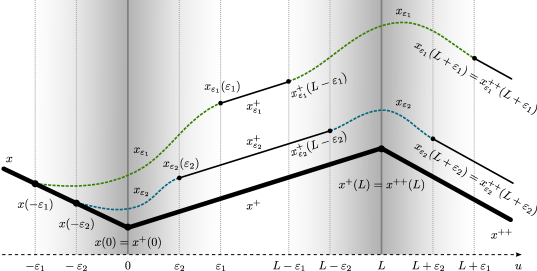
Figure 3. The limiting behaviour of the complete geodesics $\gamma_{\varepsilon}$ with two values of the regularisation parameter $0<\varepsilon_{2}<\varepsilon_{1}$ exemplified. The $x$-components of the seed and limiting geodesics are drawn in bold black, the regularised geodesics given by Proposition 5.1 are drawn dotted in green ($x_{\varepsilon_{1}}$) and blue ($x_{\varepsilon_{2}}$), respectively. Note that $x_{\varepsilon}(\varepsilon)$ converges to $x(0)$ for $\varepsilon\searrow 0$ and similarly, ${x}_{\varepsilon}(L+\varepsilon)\to x^{+}(L)$.

In this final section we investigate the limiting behaviour of the complete regularised geodesics $\gamma_{\varepsilon}$ provided by Theorem 5.3 as the regularisation parameter $\varepsilon$ goes to zero. Physically this amounts to calculating the geodesics of the impulsive full pp-wave metric (44). In fact this is only interesting if the geodesics are not parallel to or contained in the wave zone $u\in[0,L]$. So let again $\gamma=(x(s),s,r(s))$ be a ‘seed geodesic’ starting ‘in front’ of the wave zone with increasing $s$. To simplify notations we will also briefly write $\gamma=(x,r)$ and denote the data at the first impulsive surface by $\gamma(0)=(x_{0},r_{0})$ and $\dot{\gamma}(0)=(\dot{x}_{0},\dot{r}_{0})$, respectively. Clearly motivated by the procedure which leads to the completeness result in Section 5 we define the limiting geodesic $\tilde{\gamma}$ by (see also Figure 3, below)

(77) $$\tilde{\gamma}(s):=\begin{cases}\gamma(s)\qquad&(s<0)\,,\\ \gamma^{+}(s)\qquad&(0\leq s<L)\,,\\ \gamma^{++}(s)\qquad&(s\geq L)\,,\end{cases}$$

where $\gamma^{+}=(x^{+},r^{+})$ is a geodesic between the spikes, i.e., a solution of

(78) $$D_{\dot{x}}\dot{x}^{i}=-\frac{1}{L}h^{ik}(a_{k,j}-a_{j,k})\dot{x}^{j}\,,\quad\ddot{r} =\frac{1}{L}a_{(i||j)}\dot{x}^{i}\dot{x}^{j}-(h^{ik}\frac{1}{L}a_{k}(a_{i,j}-a_{j,i}))\dot{x}^{j}\,,$$

with initial data (cf. (70))

(79) $$\gamma^{+}(0) =(x_{0}^{+},r_{0}^{+}):=\lim_{\varepsilon\to 0}\gamma_{\varepsilon}(\varepsilon)=\lim_{\varepsilon\to 0}(x_{1}^{\varepsilon},r_{1}^{\varepsilon})\,,$$

(80) $$\dot{\gamma}^{+}(0) =(\dot{x}_{0}^{+},\dot{r}_{0}^{+}):=\lim_{\varepsilon\to 0}\dot{\gamma}_{\varepsilon}(\varepsilon)=\lim_{\varepsilon\to 0}(\dot{x}_{1}^{\varepsilon},\dot{r}_{1}^{\varepsilon})\,,$$

where of course $\gamma_{\varepsilon}$ is the global geodesic of Theorem 5.3 associated with the ‘seed’ $\gamma$. Furthermore, $\gamma^{++}=(x^{++},r^{++})$ is a background geodesic ‘behind’ the wave zone, i.e., $\gamma^{++}$ solves (66) with initial data (cf. (75))

(81) $$\gamma^{++}(L) =(x_{0}^{++},r_{0}^{++}):=\lim_{\varepsilon\to 0}{\gamma}(L+\varepsilon)=\lim_{\varepsilon\to 0}(x^{\varepsilon}_{3},r^{\varepsilon}_{3})\,,$$

(82) $$\dot{\gamma}^{++}(L) =(\dot{x}_{0}^{++},\dot{r}_{0}^{++}):=\lim_{\varepsilon\to 0}\dot{\gamma}(L+\varepsilon)=\lim_{\varepsilon\to 0}(\dot{x}^{\varepsilon}_{3},\dot{r}^{\varepsilon}_{3})\,.$$

Now we turn to the explicit calculation of the limits of the data (79) (80), i.e., the behaviour of the limiting geodesic at the first spike.

Proposition 6.1.

Let $\gamma_{\varepsilon}=(x_{\varepsilon},r_{\varepsilon})$ given by Theorem 5.3 with ‘seed’ $\gamma$ as above. Then

(83) $$x_{0}^{+} =x_{0}\,,\qquad\big{(}\dot{x}_{0}^{+}\big{)}^{i}=\big{(}\dot{x}_{0}\big{)}^{i}-\frac{1}{2}h^{ik}(x_{0})\big{(}\frac{2a_{k}(x_{0})}{L}-\alpha H_{,k}(x_{0})\big{)}\,,$$

(84) $$r_{0}^{+} =r_{0}+\frac{\alpha}{2}H(x_{0})\,,$$

$$\dot{r}_{0}^{+} =\dot{r}_{0}+\alpha H_{,j}(x_{0})\Big{(}\frac{\dot{x}^{j}_{0}}{2}-\frac{1}{8}h^{jk}(x_{0})\big{(}\frac{2a_{k}(x_{0})}{L}-\alpha H_{,k}(x_{0})\big{)}+h^{jk}(x_{0})a_{k}(x_{0})\Big{)}$$

(85) $$\quad+\frac{1}{2L^{2}}h^{jk}(x_{0})a_{k}(x_{0})a_{j}(x_{0})\,.$$

Proof.

We only sketch these overly technical calculations. First, $x_{0}^{+}=x_{0}$ is a direct consequence of Lemma 5.2(i). To obtain $\dot{x}_{0}^{+}$ by Lemma 5.2(ii) we only have to read off $F_{2}(x_{0})$ from (55).

For $r_{0}^{+}$ and $\dot{r}_{0}^{+}$ we use the integral equation for $r_{\varepsilon}$ with the the integral equation for $\dot{x}_{\varepsilon}$ inserted, together with the identity $\int_{-\varepsilon}^{\varepsilon}\delta_{\varepsilon}(s)\int_{-\varepsilon}^{s}\delta_{\varepsilon}(\sigma){\rm d}\sigma{\rm d}s=\frac{1}{2}$ and Lemma 5.2. We only detail this in case of $r_{0}$:

$$r_{\varepsilon}(\varepsilon)= r^{\varepsilon}_{0}+2\varepsilon\dot{r}^{\varepsilon}_{0}+\underbrace{\frac{1}{L}\int_{-\varepsilon}^{\varepsilon}\int_{-\varepsilon}^{s}\theta_{\varepsilon}Da\dot{x}_{\varepsilon}\dot{x}_{\varepsilon}{\rm d}\sigma{\rm d}s}_{\text{\sf I}}-\underbrace{\frac{1}{L^{2}}\int_{-\varepsilon}^{\varepsilon}\int_{-\varepsilon}^{s}ha\theta_{\varepsilon}^{2}Da\dot{x}_{\varepsilon}{\rm d}\sigma{\rm d}s}_{\text{\sf II}}$$

$$+\underbrace{\int_{-\varepsilon}^{\varepsilon}\int_{-\varepsilon}^{s}DH\delta^{\varepsilon}_{\alpha,\beta}\dot{x}_{\varepsilon}{\rm d}\sigma{\rm d}s}_{\text{\sf III}}-\underbrace{\frac{1}{L}\int_{-\varepsilon}^{\varepsilon}\int_{-\varepsilon}^{s}ha^{2}\theta_{\varepsilon}\delta^{\varepsilon}_{L^{-1},L^{-1}}{\rm d}\sigma{\rm d}s}_{\text{\sf IV}}$$

$$+\underbrace{\frac{1}{2L}\int_{-\varepsilon}^{\varepsilon}\int_{-\varepsilon}^{s}ha\theta_{\varepsilon}DH\delta^{\varepsilon}_{\alpha,\beta}{\rm d}\sigma{\rm d}s}_{\text{\sf V}}+\underbrace{\frac{1}{2}\int_{-\varepsilon}^{\varepsilon}\int_{-\varepsilon}^{s}H(\delta^{\varepsilon}_{\alpha,\beta})_{,u}{\rm d}\sigma{\rm d}s}_{\text{\sf VI}}\,,$$

where clearly I - V are $O(\varepsilon)$. For example $|\text{\sf III}|\leq 2\varepsilon\|DH\||\alpha|K(|\dot{x}_{0}|+c+K\|F_{2}\|_{\infty,I_{1}})$. Finally, we estimate VI:

$$|\text{\sf VI}-\frac{\alpha}{2}H(x_{0})| \leq\frac{1}{2}\int_{-\varepsilon}^{\varepsilon}\int_{-\varepsilon}^{s}|H(x_{\varepsilon}(\sigma))-H(x_{0})||(\delta^{\varepsilon}_{\alpha,\beta}(\sigma))_{,u}|{\rm d}\sigma{\rm d}s$$

$$\leq\frac{1}{2}\sup_{\sigma\in[-\varepsilon,\varepsilon]}|H(x_{\varepsilon}(\sigma))-H(x_{0})||\alpha|4\|\rho^{\prime}\|\,,$$

where we used that $\int_{-\varepsilon}^{\varepsilon}\int_{-\varepsilon}^{s}\delta_{\varepsilon}^{\prime}(\sigma){\rm d}\sigma{\rm d}s=1$ and $\sup_{\sigma\in[-\varepsilon,\varepsilon]}|H(x_{\varepsilon}(\sigma))-H(x_{0})|$ converges to zero by Lemma 5.2.

The most difficult case is $\dot{r}_{0}^{+}$, since $(\dot{r}_{\varepsilon})_{\varepsilon}$ is not uniformly bounded in $\varepsilon$. However, $(\dot{r}_{\varepsilon}(\varepsilon))_{\varepsilon}$ converges, as can seen as follows: As above write $\dot{r}_{\varepsilon}(\varepsilon)=\dot{r}^{\varepsilon}_{0}+\text{\sf I'}+\text{\sf II'}+\text{\sf III'}+\text{\sf IV'}+\text{\sf V'}+\text{\sf VI'}$. Then $\text{\sf I'}+\text{\sf II'}=O(\varepsilon)$ and in III’ one inserts the integral equation for $\dot{x}_{\varepsilon}$ and uses that $\int_{-\varepsilon}^{\varepsilon}\delta_{\varepsilon}(s)\int_{-\varepsilon}^{s}\delta_{\varepsilon}(\sigma){\rm d}\sigma{\rm d}s=\frac{1}{2}$. Finally, IV’ and V’ can be handled similarly and for VI’ one uses integration by parts to obtain $\frac{\alpha}{2}\int_{-\varepsilon}^{\varepsilon}\delta_{\varepsilon}^{\prime}H{\rm d}s=-\frac{\alpha}{2}\int_{-\varepsilon}^{\varepsilon}\delta DH\dot{x}_{\varepsilon}{\rm d}s$, which can be handled as III’. ∎

We see from the explicit expressions given in Proposition 6.1 that the limiting geodesic $\tilde{\gamma}$ displays the following behaviour at the first spike: The $x$-component is continuous with a finite jump in its velocity, since $\dot{x}_{0}^{+}\not=\dot{x}_{0}$ (in general). On the other hand, the $r$-component itself is discontinuous suffering a finite jump and the same is also true for its derivative. This behaviour is correlated with the fact that while $\dot{r}_{\varepsilon}$ is not uniformly bounded on $[-\varepsilon,\varepsilon]$ its value when leaving the regularisation strip $\dot{r}_{\varepsilon}(\varepsilon)$ is nevertheless uniformly bounded in $\varepsilon$.

Now we may analogously calculate the limits at the second spike to obtain

Proposition 6.2.

Let $\gamma_{\varepsilon}=(x_{\varepsilon},r_{\varepsilon})$ given by Theorem 5.3 with ‘seed’ $\gamma$ as above. Then

(86) $$x_{0}^{++} =x^{+}(L)\,,$$

(87) $$(\dot{x}_{0}^{++})^{i} =(\dot{x}^{+}(L))^{i}-\frac{1}{2}h^{ik}(x^{+}(L))\big{(}\frac{2a_{k}(x^{+}(L))}{L}-\beta H_{,k}(x^{+}(L))\big{)}\,,$$

(88) $$r_{0}^{++} =r^{+}(L)+\frac{\beta}{2}H(x^{+}(L))\,,$$

$$\dot{r}_{0}^{++} =\dot{r}^{+}(L)$$

(89) $$\quad+\beta H_{,j}(x^{+}(L))\Big{(}\frac{(\dot{x}^{+}(L))^{j}}{2}-\frac{1}{8}h^{jk}(x^{+}(L))\big{(}\frac{2a_{k}(x^{+}(L))}{L}-\beta H_{,k}(x^{+}(L))\big{)}$$

$$\qquad\qquad\qquad\quad+h^{jk}(x^{+}(L))a_{k}(x^{+}(L))\Big{)}$$

$$\quad+\frac{1}{2L^{2}}h^{jk}(x^{+}(L))a_{k}(x^{+}(L))a_{j}(x^{+}(L))\,.$$

Finally we may prove the actual convergence result, saying that the regularised complete geodesics $\gamma_{\varepsilon}$ of Theorem 5.3 converge to the limiting geodesics $\gamma$ of (77) consisting of appropriately matched geodesics of the complete background and the ‘intermediate’ region.

Theorem 6.3.

Let $\gamma_{\varepsilon}=(x_{\varepsilon},r_{\varepsilon})$ be the complete geodesic of Theorem 5.3 with ‘seed’ $\gamma$ as above. Then $\gamma_{\varepsilon}$ converges to the limiting geodesic $\tilde{\gamma}=(\tilde{x},\tilde{r})$ of (77) in the following sense:

1. $x_{\varepsilon}\to\tilde{x}$ locally uniformly,
   $\dot{x}_{\varepsilon}\to\dot{\tilde{x}}$ as distribution and
   uniformly on compact intervals not containing $t=0$ or $t=L$.

2. $r_{\varepsilon}\to\tilde{r}$ as distribution and
   in $\mathcal{C}^{1}$ on compact intervals not containing $t=0$ or $t=L$.

Observe that the notions of convergence in the theorem are optimal given the regularity of the limits: $\dot{\tilde{x}}$ is discontinuous at $s=0$ and $s=L$ and so uniform convergence can only hold on bounded intervals not containing these two points. The same reasoning applies to $\dot{\tilde{r}}$ and its derivative.

Proof.

Let $T>0$ then on $[-T,-\varepsilon]$ the regularised geodesic $\gamma_{\varepsilon}$ is equal to the ‘seed geodesic’ $\gamma$ since both solve the same initial value problem.

Now on $[\varepsilon,T]$ with $T\leq L-\varepsilon$ (the first spike), $\gamma_{\varepsilon}$ and $\gamma^{+}$ solve the same ODE, i.e., (78) but with different initial conditions. By continuous dependence of the solutions of ODEs on initial data we have for $t\in[\varepsilon,T]$

(90) $$\max(|\gamma_{\varepsilon}(t)-\gamma^{+}(t)|,|\dot{\gamma}_{\varepsilon}(t)-\dot{\gamma}^{+}(t)|)\leq\max(|\gamma_{\varepsilon}(\varepsilon)-\gamma^{+}(\varepsilon)|,|\dot{\gamma}_{\varepsilon}(\varepsilon)-\dot{\gamma}^{+}(\varepsilon)|)e^{LT}\,,$$

where $L$ is a Lipschitz constant for the ($\varepsilon$-independent) right-hand-side of (78) (on some suitable bounded set). Now we can insert $\gamma^{+}(0)$ to obtain

(91) $$|\gamma_{\varepsilon}(\varepsilon)-\gamma^{+}(\varepsilon)|\leq|\gamma_{\varepsilon}(\varepsilon)-\gamma^{+}(0)|+|\gamma^{+}(0)-\gamma^{+}(\varepsilon)|\to 0\,,$$

since $\gamma^{+}(0)=\lim_{\varepsilon\searrow 0}\gamma_{\varepsilon}(\varepsilon)$ and $\gamma^{+}$ is continuous. Analogously, we insert $\dot{\gamma}^{+}(0)$ to obtain

(92) $$|\dot{\gamma}_{\varepsilon}(\varepsilon)-\dot{\gamma}^{+}(\varepsilon)|\leq|\dot{\gamma}_{\varepsilon}(\varepsilon)-\dot{\gamma}^{+}(0)|+|\dot{\gamma}^{+}(0)-\dot{\gamma}^{+}(\varepsilon)|\to 0\,,$$

since $\dot{\gamma}^{+}(0)=\lim_{\varepsilon\searrow 0}\dot{\gamma}_{\varepsilon}(\varepsilon)$ and by the continuity of $\dot{\gamma}^{+}$. This gives uniform convergence of $(\gamma_{\varepsilon})_{\varepsilon}$ on any compact interval not containing $t=0$ (in its interior).

On $[-\varepsilon,\varepsilon]$ Lemma 5.2 yields the convergence of $(x_{\varepsilon})_{\varepsilon}$ to $x_{0}$ and to establish the global distributional convergence of $(r_{\varepsilon})_{\varepsilon}$ it remains only to consider $(r_{\varepsilon})_{\varepsilon}$ on $[-\varepsilon,\varepsilon]$. So let $\phi\in{\mathcal{D}}({\mathbb{R}})$ and by Lemma 5.4 there is a $C>0$ such that $|r_{\varepsilon}(t)|\leq C$ and thus

(93) $$|\int_{-\varepsilon}^{\varepsilon}(r_{\varepsilon}(s)-\tilde{r}(s))\phi(s){\rm d}s|\leq 2\varepsilon C\|\phi\|_{\infty}\to 0\,.$$

Finally, the second spike, i.e., $[L-\varepsilon,L+\varepsilon]$, and behind the wave zone, i.e., $(L+\varepsilon,\infty)$, can be handled analogously. ∎

7. Conclusion

In this contribution we have provided completeness results both for the extended as well as for the impulsive case of full pp-waves. This class of geometries allows for an arbitrary $n$-dimensional Riemannian manifold $N$ as a wave surface and for non-trivial off-diagonal terms in the metric (encoding the internal spin of the source), hence includes as special cases classical pp-waves, N-fronted waves with parallel rays, and gyratons alike. In the extended case we have generalised the results on NPWs by providing a sufficient criterion for completeness in terms of the spatial asymptotics of the metric functions with a certain (local) uniformity with respect to proper time. In the impulsive case we have employed a regularisation approach to prove that all these geometries are complete (provided the spatial profile functions are smooth). This confirms earlier results saying that the effect of the spatial asymptotics of the metric functions on completeness is wiped out in the impulsive limit. Finally we have explicitly derived the geodesics in the impulsive case in terms of a matching of corresponding background geodesics. This result, in particular, allows to derive the particle motion in the field of specific ultrarelativistic particles possessing an internal spin opening the road to applications in quantum scattering and high energy physics.

References

- [AM78] R. Abraham and J. E. Marsden. Foundations of mechanics. Benjamin/Cummings Publishing Co., Inc., Advanced Book Program, Reading, Mass., 1978. Second edition, revised and enlarged, With the assistance of Tudor Raţiu and Richard Cushman.
- [AS71] P. C. Aichelburg and R. U. Sexl. On the gravitational field of a massless particle. J. Gen. Rel. Grav., 2:303–312, 1971.
- [BEE96] J. K. Beem, P. E. Ehrlich, and K. L. Easley. Global Lorentzian geometry, volume 202 of Monographs and Textbooks in Pure and Applied Mathematics. Marcel Dekker, Inc., New York, second edition, 1996.
- [Bon70] W. B. Bonnor. Spinning null fluid in general relativity. Int. J. Theor. Phys., 3:257–266, 1970.
- [Bri25] H. W. Brinkmann. Einstein spaces which are mapped conformally on each other. Mathematische Annalen, 94(1):119–145, 1925.
- [CFS03] A. M. Candela, J. L. Flores, and M. Sánchez. On general plane fronted waves. Geodesics. Gen. Relativity Gravitation, 35(4):631–649, 2003.
- [CFS04] A. M. Candela, J. L. Flores, and M. Sánchez. Geodesic connectedness in plane wave type spacetimes. A variational approach. In Dynamic systems and applications. Vol. 4, pages 458–464. Dynamic, Atlanta, GA, 2004.
- [CG12] P. T. Chruściel and J. D. E. Grant. On Lorentzian causality with continuous metrics. Classical Quantum Gravity, 29(14):145001, 32, 2012.
- [Col85] J.-F. Colombeau. Elementary introduction to new generalized functions, volume 113 of North-Holland Mathematics Studies. North-Holland Publishing Co., Amsterdam, 1985. Notes on Pure Mathematics, 103.
- [CRS12] A. M. Candela, A. Romero, and M. Sánchez. Remarks on the completeness of trajectories of accelerated particles in riemannian manifolds and plane waves. In Proc. Int. Meeting on Differential Geometry” (Córdoba, November 15-17, 2010), pages 27–38. Univ. of Córdoba, Spain, 2012.
- [CRS13] A. M. Candela, A. Romero, and M. Sánchez. Completeness of the trajectories of particles coupled to a general force field. Arch. Ration. Mech. Anal., 208(1):255–274, 2013.
- [EE92a] P. E. Ehrlich and G. G. Emch. The conjugacy index and simple astigmatic focusing. In Geometry and nonlinear partial differential equations (Fayetteville, AR, 1990), volume 127 of Contemp. Math., pages 27–39. Amer. Math. Soc., Providence, RI, 1992.
- [EE92b] P. E. Ehrlich and G. G. Emch. Gravitational waves and causality. Rev. Math. Phys., 4(2):163–221, 1992.
- [EE93] P. E. Ehrlich and G. G. Emch. Geodesic and causal behavior of gravitational plane waves: astigmatic conjugacy. In Differential geometry: geometry in mathematical physics and related topics (Los Angeles, CA, 1990), volume 54 of Proc. Sympos. Pure Math., pages 203–209. Amer. Math. Soc., Providence, RI, 1993.
- [FF05] V. P. Frolov and D. V. Fursaev. Gravitational field of a spinning radiation beam pulse in higher dimensions. Phys. Rev. D, 71:104034, 2005.
- [Fil88] A. F. Filippov. Differential equations with discontinuous righthand sides, volume 18 of Mathematics and its Applications (Soviet Series). Kluwer Academic Publishers Group, Dordrecht, 1988. Translated from the Russian.
- [FIZ05] V. P. Frolov, W. Israel, and A. Zelnikov. Gravitational field of relativistic gyratons. Phys. Rev. D (3), 72(8):084031, 11, 2005.
- [FPV88] V. Ferrari, P. Pendenza, and G. Veneziano. Beam-like gravitational waves and their geodesics. Gen. Relativity Gravitation, 20(11):1185–1191, 1988.
- [FS03] J. L. Flores and M. Sánchez. Causality and conjugate points in general plane waves. Classical Quantum Gravity, 20(11):2275–2291, 2003.
- [FS06] J. L. Flores and M. Sánchez. On the geometry of pp-wave type spacetimes. In Analytical and numerical approaches to mathematical relativity, volume 692 of Lecture Notes in Phys., pages 79–98. Springer, Berlin, 2006.
- [FZ06] V. P. Frolov and A. Zelnikov. Gravitational field of charged gyratons. Classical Quantum Gravity, 23(6):2119–2128, 2006.
- [GKOS01] M. Grosser, M. Kunzinger, M. Oberguggenberger, and R. Steinbauer. Geometric theory of generalized functions with applications to general relativity, volume 537 of Mathematics and its Applications. Kluwer Academic Publishers, Dordrecht, 2001.
- [Gor70] W. B. Gordon. On the completeness of Hamiltonian vector fields. Proc. Amer. Math. Soc., 26:329–331, 1970.
- [GP09] J. B. Griffiths and J. Podolský. Exact space-times in Einstein’s general relativity. Cambridge Monographs on Mathematical Physics. Cambridge University Press, Cambridge, 2009.
- [KS99a] M. Kunzinger and R. Steinbauer. A note on the Penrose junction conditions. Classical Quantum Gravity, 16(4):1255–1264, 1999.
- [KS99b] M. Kunzinger and R. Steinbauer. A rigorous solution concept for geodesic and geodesic deviation equations in impulsive gravitational waves. J. Math. Phys., 40(3):1479–1489, 1999.
- [KSSV15] M. Kunzinger, R. Steinbauer, M. Stojković, and J. A. Vickers. Hawking’s singularity theorem for -metrics. Classical Quantum Gravity, 32(7):075012, 19, 2015.
- [Kun61] W. Kundt. The plane-fronted gravitational waves. Z. Physik, 163:77–86, 1961.
- [Kun62] W. Kundt. Exact solutions of the fields equations: twist-free pure radiation fields. Proc. Roy. Soc. Ser. A, 270:328–334, 1962.
- [LSŠ14] A. Lecke, R. Steinbauer, and R. Švarc. The regularity of geodesics in impulsive -waves. Gen. Relativity Gravitation, 46(1):Art. 1648, 8, 2014.
- [Min15] E. Minguzzi. Completeness of first and second order ODE flows and of Euler-Lagrange equations. J. Geom. Phys., 97:156–165, 2015.
- [OPP13] M. Ortaggio, V. Pravda, and A. Pravdová. Algebraic classification of higher dimensional spacetimes based on null alignment. Classical and Quantum Gravity, 30(1):013001, 2013.
- [Pen65a] R. Penrose. Gravitational collapse and space-time singularities. Phys. Rev. Lett., 14:57–59, 1965.
- [Pen65b] R. Penrose. A remarkable property of plane waves in general relativity. Rev. Modern Phys., 37:215–220, 1965.
- [Pen72] R. Penrose. The geometry of impulsive gravitational waves. In General relativity (papers in honour of J. L. Synge), pages 101–115. Clarendon Press, Oxford, 1972.
- [Per59] A. Peres. Some gravitational waves. Phys. Rev. Lett., 3:571–572, Dec 1959.
- [PG98] J. Podolský and J. B. Griffiths. Boosted static multipole particles as sources of impulsive gravitational waves. Phys. Rev. D (3), 58(12):124024, 5, 1998.
- [PŠ13] J. Podolský and R. Švarc. Explicit algebraic classification of Kundt geometries in any dimension. Classical and Quantum Gravity, 30(12):125007, 2013.
- [PSŠ14] J. Podolský, R. Steinbauer, and R. Švarc. Gyratonic waves and their impulsive limit. Phys. Rev. D, 90:044050, 2014.
- [PSSŠ15] J. Podolský, C. Sämann, R. Steinbauer, and R. Švarc. The global existence, uniqueness and -regularity of geodesics in nonexpanding impulsive gravitational waves. Classical Quantum Gravity, 32(2):025003, 23, 2015.
- [PSSŠ16] J. Podolský, C. Sämann, R. Steinbauer, and R. Švarc. The global uniqueness and -regularity of geodesics in expanding impulsive gravitational waves. Classical Quantum Gravity, 33(21):215006, 2016.
- [PV98] J. Podolský and K. Veselý. Chaos in -wave spacetimes. Phys. Rev. D (3), 58(8):081501, 4, 1998.
- [PV99] J. Podolský and K. Veselý. Smearing of chaos in sandwich pp-waves. Classical Quantum Gravity, 16(11):3599–3618, 1999.
- [Säm16] C. Sämann. Global hyperbolicity for spacetimes with continuous metrics. Annales Henri Poincaré, 17(6):1429–1455, 2016.
- [Sbi15] J. Sbierski. The -inextendibility of the Schwarzschild spacetime and the spacelike diameter in Lorentzian Geometry. 2015. to appear in Journal of Differential Geometry arXiv:1507.00601 [gr-qc].
- [SS12] C. Sämann and R. Steinbauer. On the completeness of impulsive gravitational wave spacetimes. Classical Quantum Gravity, 29(24):245011, 11, 2012.
- [SS15] C. Sämann and R. Steinbauer. Geodesic completeness of generalized space-times. In Pseudo-differential operators and generalized functions, volume 245 of Oper. Theory Adv. Appl., pages 243–253. Birkhäuser/Springer, Cham, 2015.
- [SSLP16] C. Sämann, R. Steinbauer, A. Lecke, and J. Podolský. Geodesics in nonexpanding impulsive gravitational waves with , Part I. Classical and Quantum Gravity, 33(11):115002, 2016.
- [Wei52] J. Weissinger. Zur Theorie und Anwendung des Iterationsverfahrens. Mathematische Nachrichten, 8(1):193–212, 1952.
- [YZF07] H. Yoshino, A. Zelnikov, and V. P. Frolov. Apparent horizon formation in the head-on collision of gyratons. Phys. Rev. D, 75(12):124005, 21, 2007.