Template matching method for the analysis of interstellar cloud structure

Abstract

Context. The structure of interstellar medium can be characterised at large scales in terms of its global statistics (e.g. power spectra) and at small scales by the properties of individual cores. Interest has been increasing in structures at intermediate scales, resulting in a number of methods being developed for the analysis of filamentary structures.

Aims. We describe the application of the generic template-matching (TM) method to the analysis of maps. Our aim is to show that it provides a fast and still relatively robust way to identify elongated structures or other image features.

Methods. We present the implementation of a TM algorithm for map analysis. The results are compared against rolling Hough transform (RHT), one of the methods previously used to identify filamentary structures. We illustrate the method by applying it to $Herschel$ surface brightness data.

Results. The performance of the TM method is found to be comparable to that of RHT but TM appears to be more robust regarding the input parameters, for example, those related to the selected spatial scales. Small modifications of TM enable one to target structures at different size and intensity levels. In addition to elongated features, we demonstrate the possibility of using TM to also identify other types of structures.

Conclusions. The TM method is a viable tool for data quality control, exploratory data analysis, and even quantitative analysis of structures in image data.

1 Introduction

The characterisation of the structure of interstellar medium (ISM) is difficult because of its complexity. The structures do not generally follow any simple patterns that could be easily parameterised. The overall properties of interstellar medium can be examined using general statistics such as the distribution of column density values ($P(D)$ analysis) (e.g. Kainulainen et al. 2009; Schneider et al. 2015), power spectra and structure functions (e.g. Armstrong et al. 1981; Green 1993; Gautier et al. 1992; Padoan et al. 2002, 2003), or fractal analysis (e.g. Scalo 1990; Elmegreen 1997). These methods do not directly provide information on the shapes of individual objects, only on the global statistics of a field.

Regarding individual structures, the analysis has concentrated on the smallest scales, on individual clumps and pre-stellar and protostellar cores (e.g. Andre et al. 1996; Motte et al. 1998; Ward-Thompson et al. 1999; Schneider et al. 2002; Könyves et al. 2010). Because of the approximate balance of gravity and supporting forces, the shapes at the smallest scales may be approximated with one-dimensional density profiles or simple 2D shapes such as 2D Gaussians (e.g. Stutzki & Guesten 1990; Lada et al. 1991; Myers et al. 1991), although the apparent simplicity is sometimes related to the finite resolution of observations.

Recently the interest in the intermediate, better resolved scales has increased. The interstellar cloud filaments imaged by the Herschel Space Observatory (Pilbratt et al. 2010) are one example of this. In the nearby star-forming regions even the internal structure of filaments can be resolved (Arzoumanian et al. 2011; Juvela et al. 2012a) and detection of filamentary structures is possible up to kiloparsec distances. In the context of interstellar clouds, the importance of filaments is partly connected to the role they play in star formation (André et al. 2014). However, filamentary structures can be detected in almost any kind of astronomical sources, from the Sun to the distant universe, in both continuum and line data.

Several methods have been used to identify and to characterise elongated structures from 3D data (usually simulations), line observations (position-position-velocity data), and two-dimensional images. An incomplete list of methods includes DisPerSe (Sousbie 2011; Arzoumanian et al. 2011) and getfilaments (Men’shchikov 2013; Rivera-Ingraham et al. 2016) routines, derivative-based (Hessian) methods (Molinari et al. 2011; Schisano et al. 2014; Salji et al. 2015), curvelets and ridgelets (e.g. Starck et al. 2003), and the inertia matrix method (Hennebelle 2013). The tools vary regarding their complexity, computational cost, and the nature and detail of the information they return on the identified structures.

In this paper, we examine the performance of a simple template matching (TM) technique in the structural analysis, for detecting for example the presence of elongated (filamentary) features, in two-dimensional image data. We compare the method to rolling Hough transform (RHT), which has been used in many image analysis applications (Illingworth & Kittler 1988) and has been applied to the filament detection from HI observations (Clark et al. 2014) and from $Herschel$ continuum data (Malinen et al. 2016). RHT was selected because its basic principles are very similar to the proposed TM implementation. Both methods are used to enhance certain structural features of the input images and thus to help characterise the structures, for example, regarding the degree of angular anisotropy. Neither method is geared towards the extraction of individual sources.

Our aim is to show that TM provides a fast and yet relatively robust way to identify local anisotropy and that, with minor changes, can also be used to highlight other types of structures. The content of this paper is as follows. Section 2 gives an overview of the TM and RHT methods. Further details on our TM implementation are given in Appendices A and B. In Sect. 3 we present a series of tests where the results of RHT and our TM implementation are compared for synthetic images. We discuss the results and possible applications of the TM method in Sect. 4 before summarising our conclusions in Sect. 5.

2 Methods

2.1 Template matching

Our aim is to highlight features that are similar to a given generic pattern in the input images. Pattern matching (or pattern recognition) is a broad category of methods to identify regular features of input data (see, e.g. Manfaat et al. 1996). In particular, we follow the template matching (TM) approach (Brunelli 2009) where data are compared to only a single pattern that is also kept fixed (apart from rotation). Such templates are limited to primitive forms (e.g. gradients or elongated shapes) contrary to many computer vision applications (see, for examples, the algorithms in the OpenCV package). The data are not expected to contain exact copies of the template. Thus, each match is associated with a significance number and the process can also be seen as a form of regression (Bishop 2006).

First, we look for a way to emphasise elongated structures of a given size scale in images. We start by creating two images that are obtained by convolving the input image with Gaussian beams with full width at half maximum (FWHM) values of one and (by default) two times a given size parameter $F_{1}$. The lower resolution image is then subtracted from the higher resolution one. In the second stage, we seek structures in this difference image, that contain a limited range of spatial scales. We compare at each pixel position the data with a pre-defined template. A simple template applicable to the detection of elongated structures of excess signal (and the one that gives zero output for a flat input image) is

$$\pmatrix{-}1/3&2/3-1/3\\ -1/32/3-1/3\\ -1/32/3-1/3\\$$ (1)

The template or stencil is placed on the map and the data values for the corresponding nine positions are read from the difference image. The step size between the stencil elements is taken to be equal to the value of the $F_{1}$ parameter. Thus, $F_{1}$ determines the angular scales for which the method is most sensitive. The data values are multiplied by the corresponding template elements and the sum is interpreted as the significance $S$ of the match between the template and the data.

The template is rotated over a range of possible orientations. If the template is not symmetric, the orientation can cover 360$\degr$ and for symmetric templates, as in Eq. (1), the angle is between $-90\degr$ and $+90\degr$. For the above template, zero position angle would correspond to a vertically elongated structure (we measure position angles counter-clockwise from north). In the tests, we sample angles with a step of 3$\degr$ or less, which corresponds to a finer sampling than that suggested by Eq. (2) in Clark et al. (2014).

The procedure is repeated for each pixel position. Although the significance $S$ could be saved as a function of the position angle or calculated as a weighted average over different angles (in a way similar to RHT, see below), we simply compress the result of the analysis into two maps, one for the position angle $\theta$ of the best match (highest $S$ value) and one for the corresponding significance $S$. In our calculations, the resulting maps have the same dimensions as the input maps although the pixel size could be larger, in proportion to the $F_{1}$ value.

Direct multiplication of an input map with the template gives larger weight for pixels with larger absolute values. Thus, the $S$ values depend on the average signal level and can be sensitive to outliers. We can alternatively normalise the data under the current template by dividing these by the standard deviation of this sample of nine data points (for the current position and orientation of the template). In the normalised version (TMN) the $S$ values depend mainly on the shapes of the template and input data, less on their absolute values.

As in the case of RHT (see Sect. 2.2), the main result is the combination of the significance and position angle maps. The significance values can be used in two ways. First, one can select for plotting a certain percentage of pixels with the highest $S$ values. It is necessary to mask most noisy pixels so that the image can be inspected visually for the presence of regions with high $S$ values and coherent position angles. This is sufficient for general data exploration and works best when, as in the case of Eq. (1), the matched structure can be long compared to the size of the individual template, thus creating large continuous regions of high significance. Second, one can make quantitative estimates of the statistical significance of a given $S$ value by using the expected distribution of $S$ values. If the data only contain white noise and background fluctuations with a standard deviation of $\sigma_{0}$ at the scale $F_{1}$, the template of Eq. (1) will result in a distribution $N(0,\sqrt{2}\sigma_{0})$ of $S$ for a random position angle. Here $N(0,\sqrt{2}\sigma_{0})$ refers to a normal distribution with a mean of zero and a standard deviation of $\sqrt{2}\sigma_{0}$, which results from the sum over the nine template elements in Eq. (1). For TMN the corresponding distribution is $N(0,\sqrt{2})$ (except that the normalisation is carried out using $\sigma_{0}$ estimated from only nine data points).

The actual relationship between $S$ and statistical significance is modified by two additional factors. First, the template is matched to filtered images, that decreases the $S$ values (for $F_{1}$ larger than one pixel). Second, at each location TM selects the position angle that gives the largest $S$ value. This makes the expectation value of $S$ positive and skews the probability distribution. Thus, the real significance depends in a non-trivial way on the spectrum of background fluctuations (as a function of spatial frequency), the symmetry properties of the template, and the number of tested position angles. The mapping between $S$ and probability can be determined with a Monte Carlo simulation. For example, for pure white noise with $\sigma_{\rm pix}=1$ per pixel and with parameters $F_{1}=2$ and $F_{2}=4$ pixels, $S$ values of 1.11, 1.54, and 2.03 correspond, respectively, to 1$\sigma$, 2$\sigma$, and 3$\sigma$ detections (confidence limits of 84%, 97.7%, and 99.87%). A given percentile of $S$ values from the analysed image corresponds to a confidence limit that is equal or higher, because the presence of real structures adds a tail of high values to the $S$ distribution.

The combined significance of a continuous region with coherent position angles is higher. The probabilities associated to $S$ values can be combined in the usual manner, taking into account that estimates are independent only at distances larger than the template size. The significance is further increased by the evidence of the similarity of position angles. A random input should result in a uniform distribution of $\theta$ values, except for potential pixel discretisation effects when $F_{1}$ approaches the pixel size. The selection of the tested region itself can also bias the estimates of the combined significance. We return to the question of combined probabilities briefly in Sect. 3.2.

As a next step of the analysis, one can trace the skeletons of filamentary structures using the $S$ and $\theta$ data. This applies only to the particular template of Eq. (1) and and we do not consider this to be a part of the TM method itself. In this paper we use skeletons only for illustration purposes and to assist in testing of the method (see Sect. 3.2). Our skeleton tracing algorithm has three parameters, $S_{\rm H}$, $S_{\rm L}$, and $\Delta\theta_{\rm max}$. The pixels associated with a skeleton must all have $S>S_{\rm L}$ and there must be at least one pixel with $S>S_{\rm H}$. Furthermore, $\Delta\theta_{\rm max}$ specifies the maximum allowed change of the position angle between consecutive skeleton positions. The ridge tracing proceeds in steps of $F_{1}$, always finding the maximum $S$ value within the allowed $\Delta\theta_{\rm max}$ sector around the local estimate of the position angle.

Figure 1 uses skeletons to illustrate the qualitative effect of the selected scale and normalisation. The data are the $Herschel$ 250 $\mu$m surface brightness observations of the field G300.86-9.00 in Musca. The map is the one used in papers Juvela et al. (2015b, a). At large scales (and high column densities) the field shows a single filament. On the other hand, at small scales and lower column densities, one can also recognise faint striations that have a clearly different distribution of position angles. In the case of TMN, one must be careful that the results for faint structures are not affected by artefacts like striping. In Fig. 1, only few skeletons are aligned with the scan directions. The skeletons are drawn using $S_{\rm H}$ and $S_{\rm L}$ values that correspond to the 96% and 80% percentiles of the $S$ distribution, requiring a minimum length of $3\times F_{1}$. With these settings, even the faintest extracted structures seem to correspond to real features in the data (Fig. 1$b$).

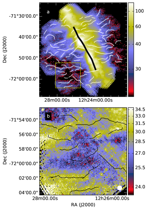
Figure 1: Filament skeletons based on TM results. The skeletons correspond to a scale of $F_{1}=0.6\arcmin$ and the TMN method except for the thick black line that shows the only skeleton found at the scale of $F_{1}=5.0\arcmin$ and without data normalisation. The background is the $Herschel$ $250\mu$m surface brightness image in units of MJy sr^-1. The lower frame shows details of a smaller region (marked with a box in the upper frame) where the $F_{1}=0.6\arcmin$ skeletons are drawn in black for better contrast.

2.2 Rolling Hough transform

We compare our TM results to the results of the RHT analysis. The RHT method is described in detail in Clark et al. (2014) so we include here only a brief overview.

The RHT procedure uses the difference of the original map and a lower resolution map that is obtained by convolving the data with a top-hat kernel with diameter $D_{\rm K}$. One examines a circular region with a diameter $D_{\rm W}$ that is centred on position $(x,y)$. One counts the number of positive pixels, $R(\theta,x,y)$, that fall under a straight line that crosses the centre point of the region and has a position angle $\theta$. Using a pre-defined parameter $Z$, the directions with the number of positive pixels below $Z\times D_{\rm W}$ are ignored. The significance of the detection of an elongated structure is described by an integral of $R(\theta,x,y)$ over 360$\degr$ and the mean position angle is obtained as

$$<\theta>=\frac{1}{2}\arctan\left(\frac{\int\sin(2\theta)R(\theta)d\theta}{\int\cos(2\theta)R(\theta)d\theta}\right).$$ (2)

This calculation of the mean position angle can be done at each pixel position or as an average over a large region. For further details, see Clark et al. (2014).

3 Results

3.1 Comparison to RHT

In this section, we apply our TM method to simulated images. The results are compared with the results of the RHT method. The images are 360$\times$360 pixels in size and the methods are set to identify elongated structures that are at least ten pixels long. Thus, in the TM method the length of the template ($2\times F$) is 10 pixels and in RHT the parameter $D_{\rm W}$ is similarly 10 pixels.

3.1.1 Elongated clumps with white noise

In the first test, we simulate a series of elongated clumps on a flat background and with white noise with standard deviation equal to 5% of the peak intensity of the structures. The intensity distribution of each clump follows a two-dimensional Plummer type profile with an additional exponential cut-off that results in a more square profile along the clump main axis. The intensities are calculated from the formula

$$I(x,y)=\left[1+(x/R_{1})^{2}+(y/R_{2})^{2}\right]^{-p}\exp(-0.05(x-R_{1})^{2}).$$ (3)

The parameters $R_{1}$ and $R_{2}$ determine the length and the width of a clump, the coordinates ($x$,$y$) having their origin at the centre of the clump.

The first frame in Fig. 2 shows the input map that contains a grid of 81 clumps of different sizes and position angles. All clumps have the same peak intensity and the value of $p=2$ but the parameters $R_{1}$ and $R_{2}$ are varied. The maximum length of the structures is about 30 pixels and the full width (measured as signal above the noise level) is at most approximately ten pixels, equal to the size of the regions analysed by both RHT and TM.

The second and the third columns of Fig. 2 show the significance (scaled between zero and one) and position angle maps. All quantities are calculated pixel by pixel, without any spatial averaging. Exact position angles are usually recovered only close to the clump centre line. For RHT, the angles tend to zero whenever the signal is low, in weak clumps and in the outer parts of all clumps. For TM, the angle changes by 90$\degr$ at the outer clump borders. The difference between the methods is caused by the fact that we adopt for TM the single position angle that resulted in the largest $S$ value. As shown in Fig. 2, the histograms of position angle errors are very similar between the two methods and, in particular, there is about the same number of pixels for which the correct position (within $\sim$2$\degr$) was recovered.

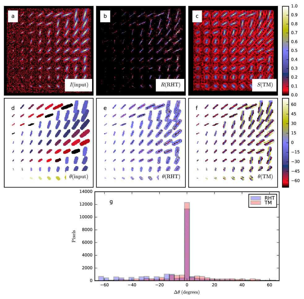
Figure 2: Comparison of RHT and TM in case of short elongated structures. Frame $a$ shows the input image and frame $d$ the position angles (in degrees) of the clump main axes. The width parameter $R_{2}$ increases from one to five across the columns of clumps. The ratio of $R_{1}/R_{2}$ (elongation) is varied between the values of two and five, the uppermost row of clumps having the largest elongation. The second and third column correspond to RHT and TM results, respectively. The RHT map of $R$ is shown in frame $b$ and the TM map of $S$ in frame $c$. The recovered position angles are shown in frames $e$ and $f$, for RHT and TM, respectively. In the second row maps pixels with the signal below the 1-$\sigma$ noise level have been masked. The frame $c$ shows histograms of position angle errors, in correspondence to the data in frames $e$ and $f$.

3.1.2 Elongated clumps on fluctuating background

In the second test we add not only white noise (again with rms noise equal to 5% of the peak intensity of the clumps) but also background fluctuations that follow a power law $k^{-2}$ as a function of the spatial frequency $k$ (spatial scales from one to 180 pixels). The results are shown in Fig. 3. We keep the parameter values of both methods the same as in the previous test of Fig. 2. For TM the values are $F_{1}$=5 pixels and $F_{2}/F_{1}=2$ and the parameters of RHT are $D_{\rm K}$=10 pixels, $D_{\rm W}$=5 pixels, and $Z$=0.6. We also checked that a change of any single RHT parameter did not lead to any significant improvement of the result.

Compared to the RHT $R$ quantity, the TM map of $S$ (Fig. 2c) shows more clearly the locations of the smallest clumps. This is partly because the input data are not thresholded, the actual values of individual pixels contribute to the $S$ values, and the signal-to-noise ratio is still relatively high. In TM the detection was done on the difference of two maps whose spatial resolutions differing only by a factor of two. Without the high pass filtering the large-scale gradients increase the dispersion of the $S$ estimates. However, in practice the effect is negligible for pixels with 10% of the highest $S$ values. TM is able to determine correct position angles within 2$\degr$ for more pixels than RHT does. There are also more pixels, for which the angles are within $\pm$20%. Even these estimates are still useful because the error is well below the standard deviation of $52\degr$, which applies to completely random angles that are limited to within 90$\degr$ of a given direction.

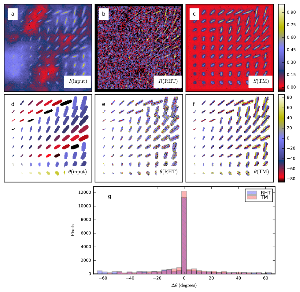
Figure 3: Comparison of RHT and TM results in the case of a fluctuating background. For the description of individual frames see Fig. 2.

3.1.3 Filaments on fluctuating background

In the final test with synthetic maps, we use simulations of long nonlinear filaments. Filaments are in this context useful as visual entities, but for both methods the calculation is carried out independently at every pixel position. The cross-filament profiles are generated using a Plummer function with exponent $p=2$, similar to Eq. (3) but as function of $y$ only. The width parameters $R_{2}$ are generated as random numbers $3\times(U(0,1)+0.5)$ (in pixel units), where $U(0,1)$ refers to uniform random numbers between zero and one. This gives a vector of $R_{2}$ parameter values that correspond to equidistant locations along the filament. The values are smoothed (as a function of the filament length) using a 1D Gaussian filter with FWHM equal to three pixels. The ridge values of the filaments are generated in a similar fashion, using random numbers $N(0,1)^{2}$ (squared simply to obtain a non-negative number) to which we apply 1D Gaussian convolution (as a function of the position along the filament) with FWHM equal to 3 pixels. $N(0,1)$ are normal distributed random numbers with a mean of zero and a standard deviation of one. The filament orientation is generated as a random process that allows rapid changes of direction. The initial position of the filament is taken from a uniform 2D distribution of positions over the map area and the initial direction of the filament is selected as a random number of $2\pi U(0,1)$ radians. We generate a vector of 240 random numbers $\theta=0.2\times N(0,1)$ and carry out 1D Gaussian convolution of this vector using a filter with a standard deviation $\sigma=$4. The elements of the $\theta$ vector are then interpreted as directions of 240 consecutive steps along the filament, each with a length of 0.5 pixels. Finally, each filament is shifted so that it is contained within the map area.

Figure 4 shows one simulation. The noise level is higher than in the previous examples and its standard deviation is equal to 16% of the expectation value of the mean intensity along the filament ridges. Therefore, the significance maps are less reliable and not all pixels above even a high percentile point necessarily belong to a real filament. The histograms in Fig. 4g are plotted for the intersection of two sets of pixels, those that are above the 95% percentile of significance (given by the $R$ and $S$ values) and those that coincide with a real filament (see Fig. 4d). The RHT parameters are this time optimised manually, only keeping $D_{\rm W}$=10 fixed. This leads to values $D_{\rm K}$=5 and $Z$=0.65. By visual inspection of the results, TM is slightly more successful in highlighting the location of filaments (Fig. 4c) and estimating their position angles (Fig. 4g).

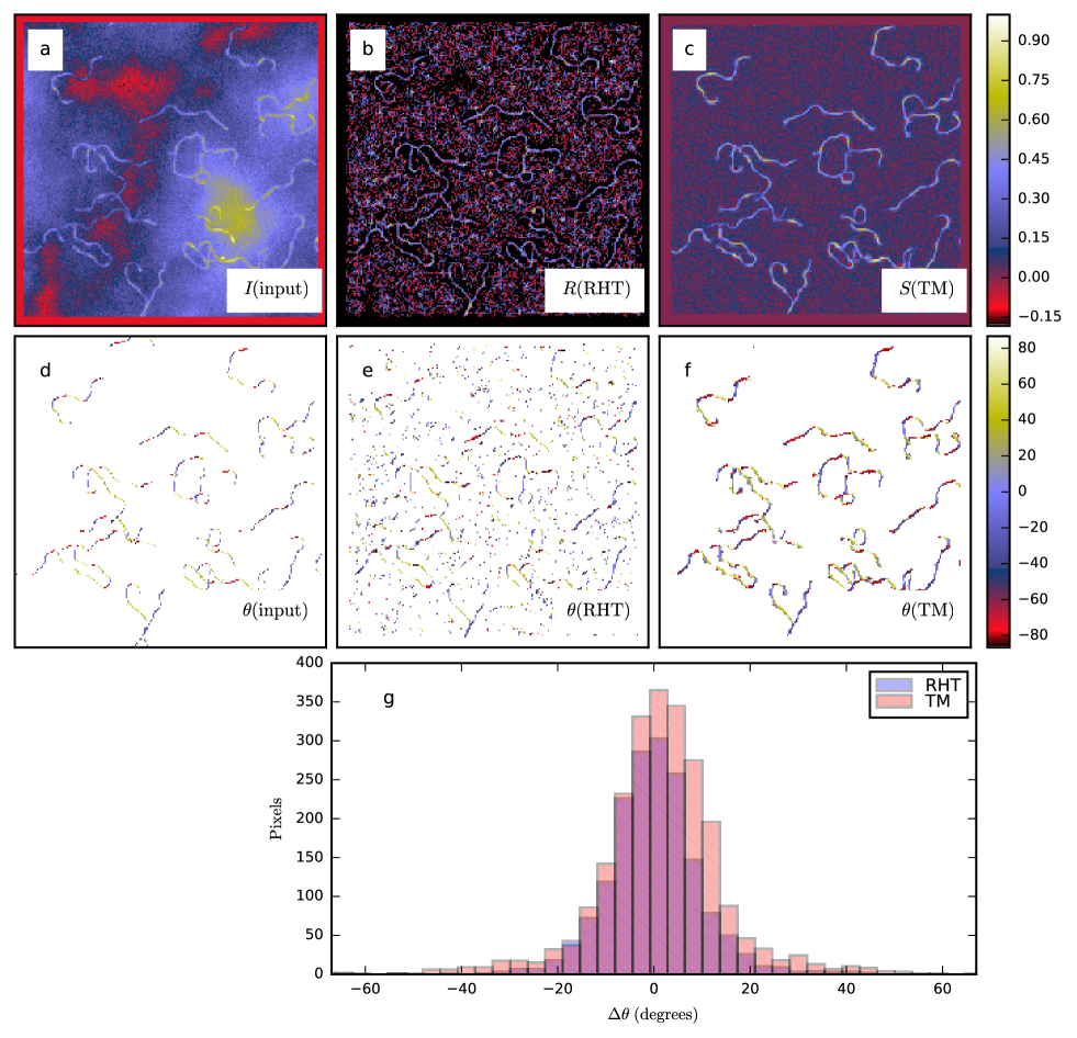
Figure 4: Comparison of RHT and TM results in the case of nonlinear filamentary structures on a fluctuating background. For the description of individual frames see Fig. 2.

Figure 5 shows how the results change as a function of the parameter values. For TM, the values of $F_{1}$ and $F_{2}/F_{1}$ are varied in 30% steps. For RHT, the parameter $Z$ is kept at a value of 0.65, which was found to give the best results in Fig. 4, but $D_{\rm W}$ and $D_{\rm K}$ are also change in 30% steps around the best parameter combination. The results of TM are less sensitive to these changes in the input parameters.

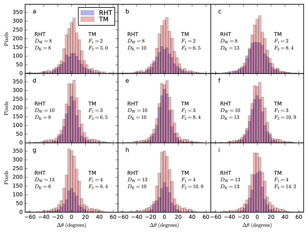
Figure 5: Change in RHT and TM results as a function of the method parameters. RHT parameters $D_{\rm W}$ and $D_{\rm K}$ are varied and parameter $Z$ is kept at a value of 0.65.

3.2 Reliability and completeness

We address questions of TM reliability estimation in the case of the simulation shown in Fig. 4. $F_{1}$ equals 2.8 pixels and any two estimates that are separated by approximately five pixels can be considered independent. We first analyse maps similar to those in Fig. 4 but without filaments and with different realisations of noise and of large-scale fluctuations. According to this Monte Carlo exercise, 84%, 97.7%, and 99.9% confidence limits correspond to $S$ values of 0.0457, 0.0638, and 0.0850, respectively. This can be compared to the $S$ values of the same percentiles that are obtained directly from the input map of Fig. 4. Those values are 0.057, 0.23, and 0.43 and they would thus result in lower estimates of the statistical significance of a given $S$ value. For example, $S=0.057$, the apparent value corresponding to the 84% confidence limit, is in reality closer to the 97.7% confidence limit. The $S$ values are higher because of the presence of real elongated structures. The more real structures the map has, the more conservative are the $S$ limits derived from the statistics of the image itself.

For a 360$\times$360 pixel image, one would expect 2981 spurious pixels above the given threshold of $S_{0}=0.0638$. We count as spurious all pixel whose distance to real filaments exceeds three pixels. The number of such pixels is 3174, by 6.5% higher than expected. However, there are still some pixels with $S>S_{0}$ that are associated to filaments but are at distances exceeding three pixels. This suggests that the $S_{0}$ threshold obtained from the Monte Carlo simulations gives a rather accurate estimate of the reliability. For the 97.7% confidence limit, we expect the map to contain 68 instances where two spurious detections are at a distance of $F_{1}$ of each other. Additionally, their position angles would also be expected to match, for example, by $2\degr$ only once per map. Thus, even the 97.7% confidence limit should in practice lead to a high probability for any structure that extends over several template lengths.

The second point we examine is the completeness of detections along the filament ridges and the rms error of the corresponding position angle estimates. For this purpose, we use filament skeletons extracted using parameters $S_{\rm H}=0.0850$ and $S_{\rm L}=0.0638$, and $\Delta\theta_{\rm max}=45\degr$. The completeness, defined as the fraction of the length of true filaments matched by a recovered skeleton within $\pm$3 pixel distance, is 95.2%. We do not show a figure of the skeletons, which closely match the filaments that are seen in the input map in Fig. 4. The rms error of the position angle estimates along the recovered skeleton is 17.5$\degr$. The number includes the larger errors from the locations of filament crossings. It could also be affected by imperfections in the filament tracking but the rms error is not lower if calculated for pixels along the true filament ridge. It is possible to reduce the position angle errors further by using the information that is contained in the $S$ map and that is also carried on to the skeletons. However, in our case we trace the skeleton only at steps of $F_{1}$ and at an accuracy of one pixel. This is not sufficient for accurate estimates of the local tangential direction, especially in the present case where the filaments exhibit rapid changes of direction.

4 Discussion

The template matching (TM) approach was found to provide a simple way to locate and to highlight pre-defined features in image data. A comparison with RHT demonstrated that the TM method is efficient in identifying elongated structures and in estimating their orientation. This is at least partly a result of the decision not to threshold the data that are used to calculate the significance values. The tested maps (both simulated and real observations) had a relatively high signal-to-noise ratio and data quantisation (via thresholding, as in the case of RHT) would result in loss of information.

We carried out tests with and without normalisation of data with its standard deviation. Without normalisation, the results are closer to RHT and the extraction concentrates on the highest intensity structures. In $Herschel$ maps, a surprising amount of detail is revealed even in diffuse regions when data normalisation is used. This is the case for example in Fig. 8 that corresponds to the lowest column densities $N({\rm H}_{2})$ of only a few times 10²⁰ cm^-2. The coherence of the position angles, which usually extends over a distance of several times the size of the template, strongly suggests that a large fraction of all plotted image pixels belong to real structures. Thus, TM can be used not only to highlight individual structures but also to demonstrate general anisotropy of the surface brightness or column density distribution.

We concentrated on the TM results computed for each pixel position separately. The visual inspection of the results was based on $S$ and $\theta$ maps thresholded at a given $S$ level. A low $S$ limit means that images also contain spurious individual pixels (pixels that are above the threshold but are not related to any significant structure). However, the human eye is good in recognising coherence, that is, separating potentially significant features from the noise. Images may also show general anisotropy that is visible in the presence of numerous faint features, none of which are significant individually. This can be sufficient for a qualitative characterisation of images when TM is applied simply as a pre-filter. However, as discussed in Sect. 2.1, it is also possible to derive quantitative estimates of the statistical significance of individual $S$ values.

In the case of the filament template, the skeletons of the filaments can be traced based on the information contained in the $S$ and $\theta$ maps (e.g, in Fig. 1) but this involves additional choices (for example, minimum $S$ values accepted in a filament or maximum allowed changes of $\theta$) beyond the pure TM method. The results of TM already point to the presence of overlapping filaments (see, for example, Fig.8) that should be common for any long line of sight through the interstellar medium. Ideally, filament tracing would be able to handle also the case of crossing filaments, retaining their identity as separate objects (see Breuer & Nikoloski 2016). In practice, the distinction between a sharp turn of a filament and the crossing of two filaments is not easy to make. Once a structure (e.g. a skeleton) has been extracted, its reliability as a separate object can be evaluated based on the $S$ values of the individual pixels and (depending on the template) the continuity of the position angle estimates (see Sect. 3.2).

We have presented results for selected scales that in the case of $Herschel$ maps ranged from 18$\arcsec$ to 5$\arcmin$. However, TM could be run routinely for the full range of scales from data resolution to the scale of the entire image. At each resolution, one could also make use of all available data that may exist for different frequency bands. The $S$ and $\theta$ maps of individual images could be combined, for example, by calculating averaged $\theta$ values weighted by $S$ and by calculating a combined $S$ in a way similar to the way RHT combines $R$ values of different $\theta$. If all maps are assumed to contain evidence of similar structures, the analysis could of course be carried out simply for a weighted average of the input maps. In case of $Herschel$, at scales above $40\arcsec$, one possibility is to use column density maps that are already a combination of data at several wavelengths. This would be a natural option, if the analysis targets the cloud mass distribution.

We used simulated and $Herschel$ surface brightness maps with map sizes up to about $900\times 900$ pixels. The run times of a single analysis were of the order of one second, even when the match was (somewhat excessively) repeated in an oversampled manner at each pixel position. The computational efficiency makes TM suitable for exploratory data analysis, as the first step that can then potentially point out the need for further analysis with other methods. Via position angle histograms, it is also a viable tool for the general characterisation of the anisotropy of the structures within an image. Other applications could be found in semi-automatic quality control of images where templates could be constructed to specifically detect certain kinds of artefacts. The row/column artefacts of CCD images could be one example, where a match would also need to be tested only for two position angles.

TM is a generic framework and an analysis could involve not only different scales but also combinations of the results with different templates. With minor modifications, the basic algorithm is applicable also in other dimensions, in particular for 1D and 3D data. In a future paper, we will use the TM method to characterise the general structural anisotropy of the $Herschel$ images observed in the Galactic Cold Cores project.

5 Conclusions

We have studied the use of a simple template matching (TM) algorithm to highlight structural elements in two-dimensional images. We examined the sensitivity of the method to detect elongated structures, for example, in $Herschel$ surface brightness data. In case of synthetic maps, the results were compared to those obtained with RHT. The study leads to the following conclusions:

• Template matching techniques provide a simple and yet an efficient method of image analysis in terms of both computational cost and the quality of results.

• In detection of elongated structures, TM provides results comparable to those of RHT. However, TM was found to perform better when maps contain significant noise and background fluctuations.

• Small changes of the basic algorithm (e.g. regarding data normalisation and spatial filtering) can be used to emphasise the brightest structures or to highlight structures at very faint levels.

• In the case of $Herschel$, its data quality allows the identification of filamentary structures at very low surface brightness levels, down to column densities $N({\rm H}_{2})\sim 10^{20}$ cm^-2.

Appendix A Implementation of the TM routines

As for RHT, TM is based on a simple set of operations that are repeated identically a number of times, possibly at every pixel position of the analysed image. Therefore, the method is well suited for parallel processing and for GPU computations. We have implemented the programme using the Python language. With the help of the pyOpenCL library, the main computations are carried out by separate OpenCL kernels. The kernels are compiled pieces of code that are run on a ‘device’, which can be for example a central processing unit (CPU) or a graphics processing unit (GPU) device. The code available at www.interstellarmedium.org/PatternMatching can be used for 2D FITS images. The web page includes a basic example of the use of the software.

It is possible to apply TM to maps of different pixelisation and even for all-sky maps. This could be useful both for scientific analysis and for data quality control. The method only requires that one is able to read data values at spatial offsets that are determined by the shape, scale, and orientation of the template. As an example of the feasibility of analysis of large data sets, we have run TM algorithm on the all-sky $Planck$ 857 GHz data. For 50 million pixel position the convolutions (with $F_{1}$ equal to 2$\degr$) and the template matching took a total of about 20 seconds.

Appendix B Alternative templates

Examples in Sect. 3.1 showed that TM can be used to recognise elongated structures. However, TM is a framework that enables the detection of different structural features according to the adopted template. The same basic algorithm can also be used for data with other dimensionality and thus, for example, also for 1D and 3D applications. As long as the size of the template (in terms of the number of points) is small, the method remains fast and is thus suitable for mass processing of data and for exploratory data analysis. We take as examples four 2D templates that we name filament, valley, gradient, and wedge (see Fig. 6), the first one being the one already used in this paper. These are applied to the 250 $\mu$m surface brightness data of LDN 1642 (field G210.90-36.55, see Juvela et al. 2012b; Montillaud et al. 2015) that are shown in Fig. 7.

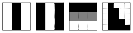
Figure 6: Examples of simple templates. From left to right: filament, valley, gradient, and wedge. The colours from white to black correspond to values 0, 0.5, and 1. In our implementation, the final pattern includes an offset that makes the sum of pattern elements zero.

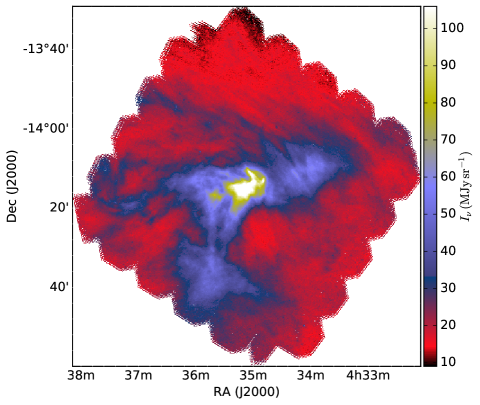
Figure 7: The 250 $\mu$m surface brightness map of the cloud L1642.

Figure 8 shows the results at scales of $F_{1}=1\arcmin$ and $F_{1}=2\arcmin$. We use data normalisation (method TMN) which, together with the spatial filtering, makes the analysis almost equally sensitive to structures at low and high surface brightness levels. We plot all pixels above the 80% percentile value of $S$. The fit is done independently at each pixel position. If the pixels form structures that are long compared to the size of the template, and especially if the estimated position angles are uniform, the combined detection can be considered reliable. Especially at the higher $1\arcmin$ resolution, the method with the filament template is able to highlight many elongated structures that are recognisable in the input data only by a very careful inspection. One can also recognise coherent patterns of elongated structures that individually are only barely visible above the noise. Figure 8 can thus be seen as an aid of exploratory data analysis although a more quantitative estimation of the reliability of individual structures is also possible (see Sect. 3.2). The map size is about $90\arcmin\times 90\arcmin$ and the images thus contain a large number of subregions that are independent at the scale of the templates.

The valley extraction is mainly complementary to the filament and sensitive not only to real elongated depressions of surface brightness but also to the edges of filaments. The gradient template is potentially more useful. Without normalisation it would identify the regions with the largest gradients, providing the absolute values and the directions of the gradients. Because in Fig. 8 we are using the method TMN, the significance $S$ now measures the linearity of the gradients rather than their magnitude.

With the last wedge template, we aim to recognise elongated structures whose width decreases at the scale of the template. It is a more specialised case (and not generic regarding the opening angle) but might be useful to highlight (for suitable input data) outflow structures or short striations extruding from a main structure. The result of wedge template is indeed found to be clearly different from, for example, the filament template and it does point out some wedge-like structures, especially when applied with $F_{1}=2\arcmin$.

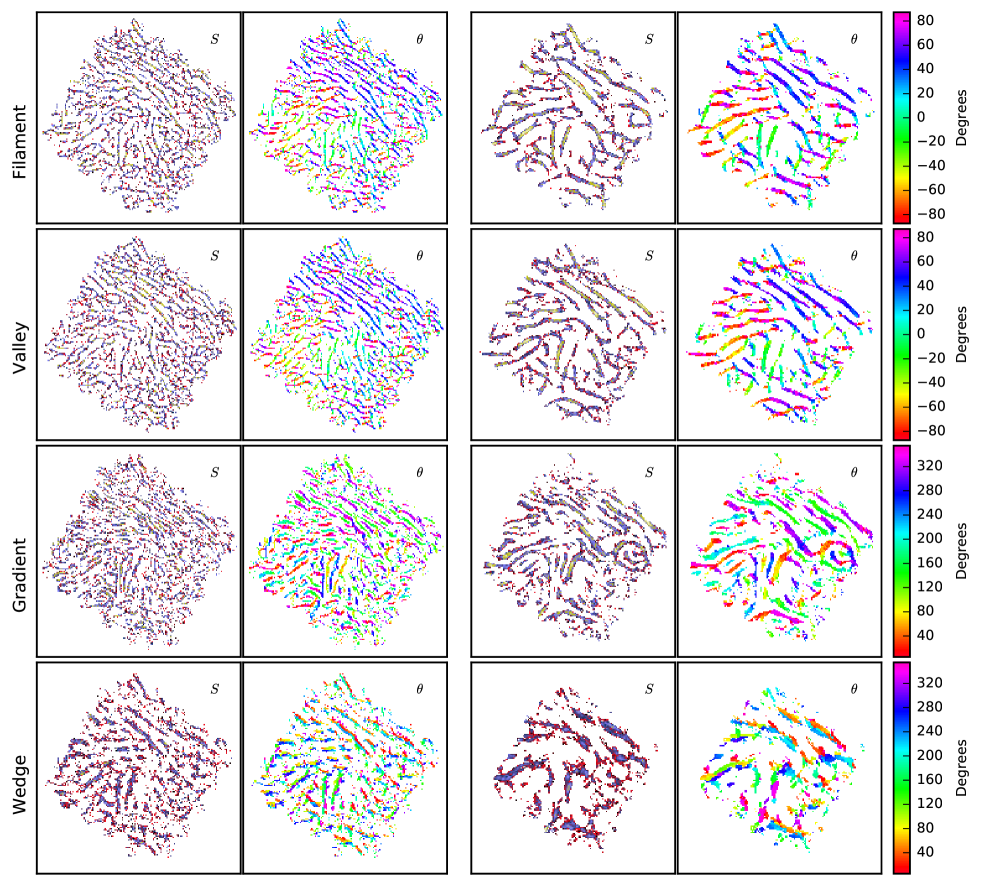
Figure 8: Results of TM using four different templates. The analysed data are the 250 $\mu$m surface brightness map of LDN 1642 in Fig. 7. The four templates (named on the left side of the figure) are depicted in Fig. 6. Each pair of frames shows the $S$ and $\theta$ maps of one extraction. On each row, the first two frames correspond to $F_{1}=1\arcmin$ and the last two frames to $F_{1}=2\arcmin$. The colour scale of $S$ maps is the same as for the position angles, with a different but a fixed numerical scale. Pixels with $S$ below the 80% percentile value have been masked.

Figure 9 shows the same results as Fig. 8 but without data normalisation. In this case, the method highlights only structures at only high intensity levels.

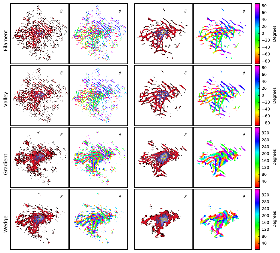
Figure 9: As Fig. 8 but without data normalisation.

References

- André et al. (2014) André, P., Di Francesco, J., Ward-Thompson, D., et al. 2014, Protostars and Planets VI, 27
- Andre et al. (1996) Andre, P., Ward-Thompson, D., & Motte, F. 1996, A&A, 314, 625
- Armstrong et al. (1981) Armstrong, J. W., Cordes, J. M., & Rickett, B. J. 1981, Nature, 291, 561
- Arzoumanian et al. (2011) Arzoumanian, D., André, P., Didelon, P., et al. 2011, A&A, 529, L6+
- Bishop (2006) Bishop, C. 2006, Pattern Recognition and Machine Learning. (Springer)
- Breuer & Nikoloski (2016) Breuer, D. & Nikoloski, Z. 2016, ArXiv e-prints [1601.00847]
- Brunelli (2009) Brunelli, R. 2009, Template matching techniques in computer vision theory and practice (Chichester, U.K: Wiley)
- Clark et al. (2014) Clark, S. E., Peek, J. E. G., & Putman, M. E. 2014, ApJ, 789, 82
- Elmegreen (1997) Elmegreen, B. G. 1997, ApJ, 486, 944
- Gautier et al. (1992) Gautier, III, T. N., Boulanger, F., Perault, M., & Puget, J. L. 1992, AJ, 103, 1313
- Green (1993) Green, D. A. 1993, MNRAS, 262, 327
- Hennebelle (2013) Hennebelle, P. 2013, A&A, 556, A153
- Illingworth & Kittler (1988) Illingworth, J. & Kittler, J. 1988, Computer vision, graphics, and image processing, 44, 87
- Juvela et al. (2015a) Juvela, M., Demyk, K., Doi, Y., et al. 2015a, A&A, 584, A94
- Juvela et al. (2012a) Juvela, M., Malinen, J., & Lunttila, T. 2012a, A&A, 544, A141
- Juvela et al. (2015b) Juvela, M., Ristorcelli, I., Marshall, D. J., et al. 2015b, A&A, 584, A93
- Juvela et al. (2012b) Juvela, M., Ristorcelli, I., Pagani, L., et al. 2012b, A&A, 541, A12
- Kainulainen et al. (2009) Kainulainen, J., Beuther, H., Henning, T., & Plume, R. 2009, A&A, 508, L35
- Könyves et al. (2010) Könyves, V., André, P., Men’shchikov, A., et al. 2010, A&A, 518, L106
- Lada et al. (1991) Lada, E. A., Bally, J., & Stark, A. A. 1991, ApJ, 368, 432
- Malinen et al. (2016) Malinen, J., Montier, L., Montillaud, J., et al. 2016, MNRAS, 460, 1934
- Manfaat et al. (1996) Manfaat, D., Duffy, A., & Lee, B. 1996, The Knowledge Engineering Review, 11, 161
- Men’shchikov (2013) Men’shchikov, A. 2013, A&A, 560, A63
- Molinari et al. (2011) Molinari, S., Schisano, E., Faustini, F., et al. 2011, A&A, 530, A133
- Montillaud et al. (2015) Montillaud, J., Juvela, M., Rivera-Ingraham, A., et al. 2015, A&A, 584, A92
- Motte et al. (1998) Motte, F., Andre, P., & Neri, R. 1998, A&A, 336, 150
- Myers et al. (1991) Myers, P. C., Fuller, G. A., Goodman, A. A., & Benson, P. J. 1991, ApJ, 376, 561
- Padoan et al. (2003) Padoan, P., Boldyrev, S., Langer, W., & Nordlund, Å. 2003, ApJ, 583, 308
- Padoan et al. (2002) Padoan, P., Cambrésy, L., & Langer, W. 2002, ApJ, 580, L57
- Pilbratt et al. (2010) Pilbratt, G. L., Riedinger, J. R., Passvogel, T., et al. 2010, A&A, 518, L1
- Rivera-Ingraham et al. (2016) Rivera-Ingraham, A., Ristorcelli, I., Juvela, M., et al. 2016, ArXiv e-prints [1603.09177]
- Salji et al. (2015) Salji, C. J., Richer, J. S., Buckle, J. V., et al. 2015, MNRAS, 449, 1782
- Scalo (1990) Scalo, J. 1990, in Astrophysics and Space Science Library, Vol. 162, Physical Processes in Fragmentation and Star Formation, ed. R. Capuzzo-Dolcetta, C. Chiosi, & A. di Fazio, 151–176
- Schisano et al. (2014) Schisano, E., Rygl, K. L. J., Molinari, S., et al. 2014, ApJ, 791, 27
- Schneider et al. (2015) Schneider, N., Bontemps, S., Girichidis, P., et al. 2015, MNRAS, 453, 41
- Schneider et al. (2002) Schneider, N., Simon, R., Kramer, C., Stutzki, J., & Bontemps, S. 2002, A&A, 384, 225
- Sousbie (2011) Sousbie, T. 2011, MNRAS, 414, 350
- Starck et al. (2003) Starck, J. L., Donoho, D. L., & Candés, E. J. 2003, A&A, 398, 785
- Stutzki & Guesten (1990) Stutzki, J. & Guesten, R. 1990, ApJ, 356, 513
- Ward-Thompson et al. (1999) Ward-Thompson, D., Motte, F., & Andre, P. 1999, MNRAS, 305, 143