Metastability of Non-reversible, Mean-field Potts Model with Three Spins

Abstract.

We examine a non-reversible, mean-field Potts model with three spins on a set with $N\uparrow\infty$ points. Without an external field, there are three critical temperatures and five different metastable regimes. The analysis can be extended by a perturbative argument to the case of small external fields. We illustrate the case of large external fields with some phenomena which are not present in the absence of external field.

1. Introduction

Some recent progress has been achieved in the potential theory of non-reversible Markov chains. Gaudillière and Landim [10] obtained a variational formula for the capacity between two disjoint sets, expressed as a double infima over flows satisfying certain boundary conditions, and Slowik [18] showed that the capacity can also be represented as a double suprema over flows satisfying a different set of boundary conditions.

These advancements permitted to describe the metastable behavior of some non-reversible dynamics. The evolution of the condensate in a totally asymmetric zero range process on a finite torus has been examined in [11], and the behavior of the ABC model among the segregated configurations in the zero temperature limit has been derived by Misturini in [15], applying the martingale method introduced in [1, 2].

In a previous paper [14], inspired by the mean-field Potts model presented in this article and based on the variational formulae alluded to above, we characterized the metastable behavior of non-reversible, continuous-time random walks in a potential field, extending to the irreversible setting results obtained by Bovier, Eckhoff, Gayrard, Klein for reversible diffusions [6, 7] and by Landim, Misturini, Tsunoda for reversible random walks in a potential field [13]. Among other results, we proved the Eyring-Kramers formula [4] for the transition rate between a metastable set and a stable set, predicted by Bouchet, Reygner [5] in the context of irreversible diffusion processes.

We examine in this article a non-reversible, mean-field Potts model [17, 19] with three spins. In the same way as the mean-field Ising model is mapped to a nearest-neighbor, one-dimensional random walk on a potentiel field [9], the dynamics of the mean-field Potts model can be mapped to a non-reversible random walk on a two-dimensional simplex.

If there is no external magnetic field, three critical temperatures and five different metastable regimes are observed. We refer to Figure 4 for an illustration of the potential in each regime. There exists a temperature $0<T_{3}<\infty$ above which no metastable behavior is observed because in this regime the entropy prevails over the energy. If the temperature $T$ is greater than or equal to $T_{3}$, in a typical configuration, one third of the spins takes one of the possible values of the spin, and starting from any configuration the system is driven progressively to this state.

There is a second critical temperature, denoted by $T_{2}$, at which four metastable sets coexist. The first one corresponds to the configurations in which one third of the spins takes one of the possible values of the spin, while the other three correspond to the configurations in which a large majority of the spins takes one of the spins value. We call the first metastable set the entropic one, and the last three metastable sets the energetic ones. The dynamics among the metastable sets can be described by a $4$-state Markov chain whose graph has a star shape. In this reduced model, jumps from a point which represents an energetic metastable set to a similar point are not allowed. Hence, to go from an energetic point to another, the reduced chain must visit the entropic point.

In the temperature range $(T_{2},T_{3})$, there are three metastable sets which correspond, in the terminology introduced in the previous paragraph, to the energetic sets, and one stable set, the entropic set. In this regime, in an appropriate time scale, starting from an energetic set, after an exponential time, the process jumps to the stable set and their remains for ever. Therefore, this evolution can be represented by a $4$-state Markov chain whose graph has a star shape and whose center is an absorbing point.

There is a third critical temperature, denoted by $T_{1}$. At this temperature there are three metastable sets, the so-called energetic ones. These three metastable sets are separated by a unique critical point, but the Hessian of the potential at this critical point is the zero matrix. In particular, this point is not a saddle point and the approach developed in [14] is not useful to prove the metastable behavior of this dynamics. Hence, even if we believe that a metastable behavior occurs among the three energetic sets, the existing techniques do not cover this situation.

In the temperature range $(T_{1},T_{2})$, there are four metastable sets and two time scales. The entropic set is shallower than the energetic ones and in a certain time scale, starting from the entropic set, after an exponential time the process jumps with equal probability to one of the energetic sets and there remains for ever. In a longer time scale, the metastable behavior of this dynamics can be described by a $3$-state Markov chain whose graph is the complete graph.

Actually, in this range of temperatures a remarkable phenomenon occurs. Starting from one of the energetic sets, after an exponential time the chain jumps to the entropic set. Once at the entropic set, the chain immediately jumps to one of the energetic sets with equal probability, and repeat from there the evolution just described. Hence, to move from one energetic set to another, the dynamics first dismantles the spin alignment present in the energetic set, staying during a negligible amount of time in the entropic set, and then, almost instantaneously, rebuild a new alignment which can coincide with the one existing before the visit to the entropic set.

Finally, in the temperature range $(0,T_{1})$, the entropic set disappears and only the three energetic sets remain. As in the temperature range $(T_{1},T_{2})$, the evolution among these sets can be described by a $3$-state Markov chain whose graph is the complete graph. The difference with the previous case is that the three saddle points of the potential separate here the energetic sets, while in the previous case these saddle points separate the energetic sets from the entropic set.

A perturbative argument permits to extend the previous analysis to the case in which the external field is small. In this case, of course, the external field breaks the symmetry among the energetic sets, and one or two of them may be favored. Besides this fact, the qualitative behavior of the dynamics is similar to the one without external field.

The analysis of the metastable behavior of a random walk in a potential field proposed in [6, 7, 13, 14] relies on the identification of the critical points of the potential and on the characterization of the eigenvalues of the Hessian of the potential at the critical points. It is not possible, in general, to obtain explicit expressions for the critical points of the potential induced by the non-reversible, mean-field Potts model. For this reason a global rigorous investigation of the metastable behavior with non small external magnetic field is not possible. However, in the case where the direction of the magnetic field points in the direction or opposite direction of one of the three possible values of the spins, a complete description of the metastable behavior of the Potts model is possible. This is presented in the last section of the article, as well as some phenomenon not observed at zero external field which are supported by numerical computations.

2. Model and Results

2.1. Mean-field Potts Model

Let ${\mathcal{S}}=\{{\boldsymbol{v}}_{0},\,{\boldsymbol{v}}_{1},\,{\boldsymbol{v}}_{2}\}$ be the set of spins, where ${\boldsymbol{v}}_{k}=\left(\cos(2\pi k/3),\,\sin(2\pi k/3)\right)$, $0\leq k\leq 2$, and let $T_{N}=\{1,\,2,\,\dots,\,N\}$, $N\in\mathbb{N}$ be the set of sites. The configuration space, represented by $\Omega_{N}$, is the set ${\mathcal{S}}^{T_{N}}$. Denote by $\sigma=(\sigma_{1},\sigma_{2},\dots,\sigma_{N})$ the configurations of $\Omega_{N}$, where $\sigma_{i}\in{\mathcal{S}}$, $i\in T_{N}$, is the spin at the $i$-th site of $\sigma$. The Hamiltonian $\mathbb{H}_{N}:\Omega_{N}\rightarrow\mathbb{R}$ is defined by

$$\mathbb{H}_{N}(\sigma)\;=\;-\,\frac{1}{2N}\sum_{1\leq i,j\leq N}\sigma_{i}\cdot\sigma_{j}\;-\;\sum_{i=1}^{N}{\boldsymbol{h}}_{\text{e}}\cdot\sigma_{i}\;=\;-\frac{N}{2}\,\Big{|}\frac{1}{N}\sum_{i=1}^{N}\sigma_{i}\Big{|}^{2}\;-\;{\boldsymbol{h}}_{\text{e}}\cdot\sum_{i=1}^{N}\sigma_{i}\;,$$ (2.1)

where ${\boldsymbol{h}}_{\text{e}}=(r_{\text{e}}\cos\theta_{\text{e}},\,r_{\text{e}}\sin\theta_{\text{e}})$ stands for an external magnetic field, and ${\boldsymbol{x}}\cdot{\boldsymbol{y}}$ for the scalar product between ${\boldsymbol{x}}$ and ${\boldsymbol{y}}\in{\mathbb{R}}^{2}$. Here, $r_{\text{e}}\geq 0$ and $0\leq\theta_{\text{e}}<2\pi$ represent the magnitude and the angle of the external field, respectively. The model associated to this mean-field type Hamiltonian is known as the mean-field Potts Model [17]. We refer to the review paper [19] for an introduction on Potts model.

Fix $\beta>0$ and denote by $\mu_{\beta}^{N}$ the Gibbs measure associated to the Hamiltonian $\mathbb{H}_{N}$ at the inverse temperature $\beta$:

$$\mu_{\beta}^{N}(\sigma)\;=\;\frac{3^{-N}}{Z_{N}(\beta)}e^{-\beta\mathbb{H}_{N}(\sigma)}\;\;;\;\sigma\in\Omega_{N}\;,$$ (2.2)

where $Z_{N}(\beta)$ is the partition function defined by

$$Z_{N}(\beta)\;=\;3^{-N}\sum_{\sigma\in\Omega_{N}}e^{-\beta\mathbb{H}_{N}(\sigma)}$$

so that $\mu_{\beta}^{N}$ is a probability measure on $\Omega_{N}$.

2.2. Spin Dynamics

A natural dynamics for the Potts model introduced in the previous section is the one in which spins are allowed to jump only in one direction, say the counter-clockwise one: ${\boldsymbol{v}}_{k}\rightarrow{\boldsymbol{v}}_{k+1}$, $0\leq k\leq 2$, where summation in the subscript is performed modulo $3$. Denote by $\mathscr{R}:{\mathcal{S}}\rightarrow{\mathcal{S}}$ the counter-clockwise rotation on ${\mathcal{S}}$, i.e., $\mathscr{R}({\boldsymbol{v}}_{k})={\boldsymbol{v}}_{k+1}$ for $0\leq k\leq 2$, and denote by $\tau_{i}\,\sigma$, $i\in T_{N}$, the configuration obtained from $\sigma$ by rotating counter-clockwise the $i$-th spin by an angle of $(2\pi/3)$, namely,

$$(\tau_{i}\,\sigma)_{j}\;=\;\mathscr{R}(\sigma_{j})\,\mathbf{1}\{j=i\}+\sigma_{j}\,\mathbf{1}\{j\neq i\}\;.$$

Denote by ${\mathscr{L}}_{N}$ the generator which acts on functions $f:\Omega_{N}\rightarrow\mathbb{R}$ as

$$(\mathcal{L}_{N}f)(\sigma)\;=\;\frac{1}{N}\sum_{i=1}^{N}c_{i}(\sigma)\,\{f(\tau_{i}\sigma)-f(\sigma)\}\;,$$ (2.3)

where $c_{i}(\sigma)$, $i\in T_{N}$, is the jump rate given by

$$c_{i}(\sigma)\;=\;\exp\Big{\{}-\frac{\beta}{3}\sum_{k=0}^{2}\left[\mathbb{H}_{N}(\tau_{i}^{(k)}\sigma)-\mathbb{H}_{N}(\sigma)\right]\Big{\}}\;,$$ (2.4)

and where $\tau_{i}^{(k)}$, $k\geq 0$, stands for the $k$-th iterated of the operator $\tau_{i}$. These jump rates were chosen for $\mu_{\beta}^{N}$ to be the stationary state.

Denote by $\sigma(t)=(\sigma_{1}(t),\cdots,\sigma_{N}(t))$, $t\geq 0$, the continuous-time Markov chain on $\Omega_{N}$ generated by $\mathscr{L}_{N}$. Note that $\sigma(t)$ is non-reversible with respect to $\mu_{N}^{\beta}$ because of the cyclic nature of the dynamics.

2.3. Metastability

Denote by ${\mathfrak{m}}_{N}(\sigma)$ the magnetization of the configuration $\sigma\in\Omega_{N}$:

$${\mathfrak{m}}_{N}(\sigma)\;=\;\frac{1}{N}\sum_{i=1}^{N}\sigma_{i}\;.$$

In this article, we investigate the metastable behavior of the the magnetization ${\mathfrak{m}}_{N}(t):={\mathfrak{m}}_{N}(\sigma(t))$ under the dynamics defined by (2.3).

Note that the Hamiltonian (2.1) can be represented in terms of the magnetization:

$$\mathbb{H}_{N}(\sigma)\;=\;\,N\Big{[}-\frac{1}{2}\left|{\mathfrak{m}}_{N}(\sigma)\right|^{2}\;-\;{\boldsymbol{h}}_{\text{e}}\cdot{\mathfrak{m}}_{N}(\sigma)\Big{]}\;,$$ (2.5)

and that the rotation rate $c_{i}(\sigma)$ is represented only in terms of the Hamiltonian. Thereby, the process ${\mathfrak{m}}_{N}(t)$ is itself a continuous-time Markov chain on $\mathbb{R}^{2}$ and inherits the non-reversibility from the underlying spin dynamics.

It has been observed in [9, 7] that the magnetization of the mean-field, Curie-Weiss model exhibits a metastable behavior at low temperatures due to the competition between entropy and energy. The mean-field, Potts model considered in this article can be regarded as a generalization of the Curie-Weiss model, and exhibits an analogous metastable behavior at low temperatures.

A complete analysis of the metastable behavior in the case where there is no external field is presented in Section 4. As mentioned in the introduction, there exist in this case three critical inverse temperatures $\beta_{1}>\beta_{2}>\beta_{3}$, where $\beta_{i}$ stands for the inverse of the temperature $T_{i}$ referred to in Section 1. While $\beta_{1}=2$, numerical computations give that $\beta_{2}\thickapprox 1.8484$ and $\beta_{3}\thickapprox 1.8304$. At each of these critical temperatures a qualitative modification of the metastable behavior is observed.

The article is organized as follows. In Section 3, we show that the evolution of the magnetization is described by a random walk evolving in a potential field defined in a two-dimensional simplex. In Section 4, we describe all different metastable regimes in the case of zero-external field, following the martingale approach of [1, 2, 3] and based on the recent work [14]. In Section 5, by a perturbative argument, we extend these results to the case of a small external field, and we present new phenomena which occur when there is a large external field.

3. Reduction to a Cyclic Random Walk in a Potential Field

We examine in this section the dynamics of the magnetization ${\mathfrak{m}}_{N}(t)$. We show that it evolves according to a non-reversible random walk in a potential field.

Denote by $r_{N}^{k}(\sigma)$, $0\leq k\leq 2$, the ratio of sites of $\sigma\in\Omega_{N}$ whose spin is equal to ${\boldsymbol{v}}_{k}$:

$$r_{N}^{k}(\sigma)\;=\;\frac{1}{N}\sum_{i=1}^{N}\mathbf{1}\{\sigma_{i}={\boldsymbol{v}}_{k}\}\;.$$

Clearly, for all configurations $\sigma$, $\sum_{0\leq k\leq 2}r_{N}^{k}(\sigma)=1$. For this reason, denote by $\Xi$ the two-dimensional simplex given by

$$\Xi\;=\;\{{\boldsymbol{x}}=(x_{1},x_{2}):x_{1},\,x_{2}\geq 0,\,x_{1}+x_{2}\leq 1\}\subset\mathbb{R}^{2}\;,$$

and let $\Xi_{N}$ be the discretization of $\Xi$: $\Xi_{N}=\Xi\cap(\mathbb{Z}/N)^{2}$. A point $(x_{1},x_{2})$ in $\Xi$ or $\Xi_{N}$ is represented as ${\boldsymbol{x}}=(x_{1},x_{2})$, and for a point $(x_{1},x_{2})$, $x_{0}$ stands for $1-x_{1}-x_{2}$.

Let ${\boldsymbol{r}}_{N}(\sigma)=(r_{N}^{1}(\sigma),\,r_{N}^{2}(\sigma))\in\Xi_{N}$. An elementary computation shows that the magnetization can be expressed in terms of ${\boldsymbol{r}}_{N}(\sigma)$ as

$${\mathfrak{m}}_{N}(\sigma)\;=\;\psi({\boldsymbol{r}}_{N}(\sigma))\;,$$ (3.1)

where $\psi:\Xi\rightarrow\mathbb{R}^{2}$ is defined by

$$\psi({\boldsymbol{x}})\;=\;(2x_{1}+x_{2}-1){\boldsymbol{v}}_{1}+(x_{1}+2x_{2}-1){\boldsymbol{v}}_{2}\;,$$ (3.2)

which is a bijection between $\Xi_{N}$ and $\psi(\Xi_{N})$. Figure 1 illustrates this bijective relation.

Figure 1. The bijective relation between $\Xi_{N}$ and $\psi(\Xi_{N})$. The set $\psi(\Xi_{N})$ consists of the triangular lattice points of the equilateral triangle determined by the three vertices ${\boldsymbol{v}}_{0}$, ${\boldsymbol{v}}_{1}$ and ${\boldsymbol{v}}_{2}$.

Since $\psi$ is a bijection, to investigate the metastable behavior of the magnetization ${\mathfrak{m}}_{N}(t)$, it suffices to examine the evolution of ${\boldsymbol{r}}_{N}(t):={\boldsymbol{r}}_{N}(\sigma(t))$.

The dynamics of ${\boldsymbol{r}}_{N}(t)$. As $\psi$ is a bijection, ${\boldsymbol{r}}_{N}(t)$ inherits the Markov property from ${\mathfrak{m}}_{N}(t)$. We first consider the stationary state of the dynamics.

By (2.5) and (3.1), the Hamiltonian ${\mathbb{H}}_{N}(\sigma)$ can be written as

$$\mathbb{H}_{N}(\sigma)\;=\;NH({\boldsymbol{r}}_{N}(\sigma))\;,\;\;\;H({\boldsymbol{x}})\;=\;-\frac{1}{2}\left|\psi({\boldsymbol{x}})\right|^{2}-{\boldsymbol{h}}_{\text{e}}\cdot\psi({\boldsymbol{x}})\;.$$ (3.3)

Hence, the invariant measure of the chain ${\boldsymbol{r}}_{N}(t)$, denoted by $\nu_{\beta}^{N}$, can be derived from (2.2) and (3.3). More precisely, for ${\boldsymbol{x}}\in\Xi_{N}$,

$$\nu_{\beta}^{N}({\boldsymbol{x}})\;=\;\sum_{\sigma:{\boldsymbol{r}}_{N}(\sigma)={\boldsymbol{x}}}\frac{3^{-N}}{Z_{N}(\beta)}\,\exp\{-\beta\mathbb{H}_{N}(\sigma)\}\;.$$ (3.4)

Therefore, by straightforward computations and Stirling’s formula,

$$\nu_{\beta}^{N}({\boldsymbol{x}})\;=\;\frac{1}{\widehat{Z}_{N}(\beta)}\,\exp\{-\beta NF_{\beta,N}({\boldsymbol{x}})\}\;,$$ (3.5)

where $\widehat{Z}_{N}(\beta)=2\pi NZ_{N}(\beta)$ is the partition function, and where the potential $F_{\beta,N}(\cdot)$ is given by

$$F_{\beta,N}({\boldsymbol{x}})\;=\;F_{\beta}({\boldsymbol{x}})\;+\;\frac{1}{N}\,G_{\beta,N}({\boldsymbol{x}})\;.$$ (3.6)

In this equation,

$$F_{\beta}({\boldsymbol{x}})\;=\;H({\boldsymbol{x}})\;+\;\frac{1}{\beta}S({\boldsymbol{x}})\;,\quad G_{\beta,N}({\boldsymbol{x}})\;=\;\frac{\log(x_{0}x_{1}x_{2})}{2\beta}\;+\;O(N^{-1})\;,$$ (3.7)

and $S$ is the entropy function defined by

$$S({\boldsymbol{x}})\;=\;\sum_{i=0}^{2}x_{i}\thinspace\log(3x_{i})\;.$$ (3.8)

In these equations we used the convention that $\log 0=-\infty$ and that $e^{-\infty}=0$. Moreover, $G_{\beta,N}\rightarrow G_{\beta}$ uniformly on every compact subsets of $\mbox{int}(\Xi)$, where $G_{\beta}({\boldsymbol{x}})=\log(x_{0}x_{1}x_{2})/(2\beta)$.

To examine the dynamics of the chain ${\boldsymbol{r}}_{N}(t)$, denote by ${\boldsymbol{e}}_{1}=(1,0)$, ${\boldsymbol{e}_{2}}=(0,1)$ the canonical basis of $\mathbb{R}^{2}$, set ${\boldsymbol{e}}_{0}=(0,0)$, and let ${\boldsymbol{e}}_{k}^{N}=N^{-1}{\boldsymbol{e}}_{k}$, $0\leq k\leq 2$. Recall that we denote by ${\boldsymbol{v}}_{0}$, ${\boldsymbol{v}}_{1}$, ${\boldsymbol{v}}_{2}$ the three values a spin may assume and that the dynamics allows only jumps from ${\boldsymbol{v}}_{k}$ to ${\boldsymbol{v}}_{k+1}$, $0\leq k\leq 2$. A jump of spin from ${\boldsymbol{v}}_{0}$ to ${\boldsymbol{v}}_{1}$ corresponds to that of the chain ${\boldsymbol{r}}_{N}(t)$ from ${\boldsymbol{x}}$ to ${\boldsymbol{x}}+{\boldsymbol{e}}_{1}^{N}$. Since there are $Nx_{0}$ sites whose spin is ${\boldsymbol{v}}_{0}$, in view of (2.4) and (3.3), the rate at which the chain ${\boldsymbol{r}}_{N}(t)$ jumps from ${\boldsymbol{x}}$ to ${\boldsymbol{x}}+{\boldsymbol{e}}_{1}^{N}$, denoted by $R_{N}({\boldsymbol{x}},{\boldsymbol{x}}+{\boldsymbol{e}}_{1}^{N})$, is given by

$$R_{N}({\boldsymbol{x}},{\boldsymbol{x}}+{\boldsymbol{e}}_{1}^{N})\;=\;x_{0}\exp\left\{-N\beta(\overline{H}({\boldsymbol{x}})-H({\boldsymbol{x}}))\right\}\;,$$

where

$$\overline{H}({\boldsymbol{x}})\;=\;\frac{1}{3}\big{\{}H({\boldsymbol{x}})+H({\boldsymbol{x}}+{\boldsymbol{e}}_{1}^{N})+H({\boldsymbol{x}}+{\boldsymbol{e}}_{2}^{N})\big{\}}\;.$$

Similarly, a jump from ${\boldsymbol{v}}_{1}$ to ${\boldsymbol{v}}_{2}$ corresponds to a jump of the chain ${\boldsymbol{r}}_{N}$ from ${\boldsymbol{x}}$ to ${\boldsymbol{x}}-{\boldsymbol{e}}_{1}^{N}+{\boldsymbol{e}}_{2}^{N}$, while a jump from ${\boldsymbol{v}}_{2}$ to ${\boldsymbol{v}}_{0}$ corresponds to a jump from ${\boldsymbol{x}}$ to ${\boldsymbol{x}}-{\boldsymbol{e}}_{2}^{N}$. The rates can be computed easily and are given by

$$R_{N}({\boldsymbol{x}},{\boldsymbol{x}}-{\boldsymbol{e}}_{1}^{N}+{\boldsymbol{e}}_{2}^{N})\;=\;(x_{1}+N^{-1})\,\exp\left\{-N\beta(\overline{H}({\boldsymbol{x}}-{\boldsymbol{e}}_{1}^{N})-H({\boldsymbol{x}}))\right\}\;,$$

$$\quad R_{N}({\boldsymbol{x}},{\boldsymbol{x}}-{\boldsymbol{e}}_{2}^{N})\;=\;(x_{2}+N^{-1})\,\exp\left\{-N\beta(\overline{H}({\boldsymbol{x}}-{\boldsymbol{e}}_{2}^{N})-H({\boldsymbol{x}}))\right\}\;.$$

Hence, the generator ${\mathcal{L}}_{N}$ of the Markov chain ${\boldsymbol{r}}_{N}(t)$ is given by

$$({\mathcal{L}}_{N}f)({\boldsymbol{x}}) =\;R_{N}({\boldsymbol{x}},{\boldsymbol{x}}+{\boldsymbol{e}}_{1}^{N})\left[f({\boldsymbol{x}}+{\boldsymbol{e}}_{1}^{N})-f({\boldsymbol{x}})\right]$$ (3.9)

$$+\;R_{N}({\boldsymbol{x}},{\boldsymbol{x}}-{\boldsymbol{e}}_{1}^{N}+{\boldsymbol{e}}_{2}^{N})\left[f({\boldsymbol{x}}-{\boldsymbol{e}}_{1}^{N}+{\boldsymbol{e}}_{2}^{N})-f({\boldsymbol{x}})\right]$$

$$+\;R_{N}({\boldsymbol{x}},{\boldsymbol{x}}-{\boldsymbol{e}}_{2}^{N})\left[f({\boldsymbol{x}}-{\boldsymbol{e}}_{2}^{N})-f({\boldsymbol{x}})\right]\;.$$

Denote by $\mathbb{P}_{{\boldsymbol{x}}}^{N}$ the law of the Markov chain ${\boldsymbol{r}}_{N}(t)$ starting from ${\boldsymbol{x}}\in\Xi_{N}$ and by $\mathbb{E}_{{\boldsymbol{x}}}^{N}$ the associated expectation.

Cyclic random walks in a potential field. Let $\gamma^{N}$ be the cycle $({\boldsymbol{e}}_{0}^{N},{\boldsymbol{e}}_{1}^{N},{\boldsymbol{e}}_{2}^{N},{\boldsymbol{e}}_{0}^{N})$ on $(\mathbb{Z}/N)^{2}$, and denote by $\gamma_{{\boldsymbol{x}}}^{N}$ the cycle $\gamma^{N}$ translated by ${\boldsymbol{x}}\in(\mathbb{Z}/N)^{2}$, i.e., $\gamma_{{\boldsymbol{x}}}^{N}={\boldsymbol{x}}+\gamma^{N}$. Let $\widehat{\Xi}_{N}$ be the set defined by

$$\widehat{\Xi}_{N}\;=\;\{{\boldsymbol{x}}\in\Xi_{N}:\gamma_{{\boldsymbol{x}}}^{N}\subset\Xi_{N}\}\;=\;\{{\boldsymbol{x}}\in\Xi_{N}:x_{1}+x_{2}\leq 1-N^{-1}\}\;.$$

Denote by ${\mathcal{L}}_{N,{\boldsymbol{x}}}$, ${\boldsymbol{x}}\in\widehat{\Xi}_{N}$, the cycle generator on $\gamma_{{\boldsymbol{x}}}^{N}$ given by

$$({\mathcal{L}}_{N,{\boldsymbol{x}}}f)({\boldsymbol{x}}+{\boldsymbol{e}}_{i}^{N})\;=\;\widetilde{R}_{N}({\boldsymbol{x}}+{\boldsymbol{e}}_{i}^{N},{\boldsymbol{x}}+{\boldsymbol{e}}_{i+1}^{N})\left[f({\boldsymbol{x}}+{\boldsymbol{e}}_{i+1}^{N})-f({\boldsymbol{x}}+{\boldsymbol{e}}_{i}^{N})\right]\;,$$

for $0\leq i\leq 2$, where the jump rate $\widetilde{R}_{N}$ is given by

$$\widetilde{R}_{N}({\boldsymbol{x}}+{\boldsymbol{e}}_{i}^{N},{\boldsymbol{x}}+{\boldsymbol{e}}_{i+1}^{N})\;=\;\exp\{-\beta N[\,\overline{F}_{\beta,N}({\boldsymbol{x}})-F_{\beta,N}({\boldsymbol{x}}+{\boldsymbol{e}}_{i}^{N})]\}\;,$$ (3.10)

and

$$\overline{F}_{\beta,N}({\boldsymbol{x}})\;=\;\frac{1}{3}\big{\{}F_{\beta,N}({\boldsymbol{x}}+{\boldsymbol{e}}_{0}^{N})+F_{\beta,N}({\boldsymbol{x}}+{\boldsymbol{e}}_{1}^{N})+F_{\beta,N}({\boldsymbol{x}}+{\boldsymbol{e}}_{2}^{N})\big{\}}\;.$$

An elementary computation shows that for ${\boldsymbol{x}}\in\widehat{\Xi}_{N}$, $0\leq i\leq 2$,

$$R_{N}({\boldsymbol{x}}+{\boldsymbol{e}}_{i}^{N},{\boldsymbol{x}}+{\boldsymbol{e}}_{i+1}^{N})\;=\;w_{N}({\boldsymbol{x}})\,\widetilde{R}_{N}({\boldsymbol{x}}+{\boldsymbol{e}}_{i}^{N},{\boldsymbol{x}}+{\boldsymbol{e}}_{i+1}^{N})\;,$$ (3.11)

where the weights $w_{N}({\boldsymbol{x}})$, ${\boldsymbol{x}}\in\widehat{\Xi}_{N}$, are given by

$$w_{N}({\boldsymbol{x}})\;=\;\left[x_{0}\left(x_{1}+\frac{1}{N}\right)\left(x_{2}+\frac{1}{N}\right)\right]^{\frac{1}{3}}\;.$$ (3.12)

Hence, the generator ${\mathcal{L}}_{N}$ defined in (3.9) can be represented in terms of the cycle generators ${\mathcal{L}}_{N,{\boldsymbol{x}}}$, ${\boldsymbol{x}}\in\widehat{\Xi}_{N}$, as

$${\mathcal{L}}_{N}\;=\;\sum_{{\boldsymbol{x}}\in\widehat{\Xi}_{N}}w_{N}({\boldsymbol{x}})\,{\mathcal{L}}_{N,{\boldsymbol{x}}}\;.$$ (3.13)

Note that the weight function $w_{N}({\boldsymbol{x}})$ converges to $w({\boldsymbol{x}})=(x_{0}x_{1}x_{2})^{1/3}$ uniformly on every compact subsets of $\mbox{int}(\Xi)$. Thereby, the Markov chain ${\boldsymbol{r}}_{N}(t)$ is a special case of the model considered in Remark 2.9 of [14].

The potential $F_{\beta}$. The global structure of the inter-valley dynamics is essentially related to the potential $F_{\beta}$ defined in (3.7).

Denote by $\partial_{x_{i}}F_{\beta}$, $i=1,\,2$, the partial derivative of $F_{\beta}$ with respect to $x_{i}$. We have that

$$(\partial_{x_{1}}F_{\beta})({\boldsymbol{x}})\;=\;-\,\frac{3}{2}(x_{1}-x_{0})\;+\;\frac{1}{\beta}\log\frac{x_{1}}{x_{0}}\;-\;r_{\text{e}}\left[\cos\left(\theta_{\text{e}}-\frac{2\pi}{3}\right)-\cos\theta_{\text{e}}\right]\;,$$ (3.14)

$$(\partial_{x_{2}}F_{\beta})({\boldsymbol{x}})\;=\;-\,\frac{3}{2}(x_{2}-x_{0})\;+\;\frac{1}{\beta}\log\frac{x_{2}}{x_{0}}\;-\;r_{\text{e}}\left[\cos\left(\theta_{\text{e}}-\frac{4\pi}{3}\right)-\cos\theta_{\text{e}}\right]\;.$$

Therefore, a point ${\boldsymbol{x}}\in\Xi$ is a critical point of $F_{\beta}$ if and only if

$$\frac{1}{\beta}\log x_{k}\;-\;\frac{3}{2}x_{k}\;-\;r_{\text{e}}\,\cos\left(\theta_{\text{e}}-\frac{2k\pi}{3}\right)$$ (3.15)

are equal for $k=0$, $1$, $2$.

The Hessian of $F_{\beta}$, denoted by $\nabla^{2}F_{\beta}$, is given by

$$(\nabla^{2}F_{\beta})({\boldsymbol{x}})\;=\;\begin{pmatrix}\frac{1}{\beta x_{0}}+\frac{1}{\beta x_{1}}-3&\frac{1}{\beta x_{0}}-\frac{3}{2}\\ \frac{1}{\beta x_{0}}-\frac{3}{2}&\frac{1}{\beta x_{0}}+\frac{1}{\beta x_{2}}-3\end{pmatrix}\;.$$ (3.16)

4. Zero External Magnetic Field

We examine in this section the metastable behavior of the Potts model under the assumption that the magnetic field vanishes: ${\boldsymbol{h}}_{\text{e}}={\boldsymbol{0}}$.

4.1. Structure of Valleys

To describe the valleys of the potential $F_{\beta}$, we first identify in Proposition 4.2 below all critical points of $F_{\beta}$.

For a point ${\boldsymbol{x}}$ at the boundary of $\Xi$, let ${\boldsymbol{n}}({\boldsymbol{x}})$ be the exterior normal vector at ${\boldsymbol{x}}$ with respect to the domain $\Xi$. By (3.14),

$$\nabla F_{\beta}({\boldsymbol{x}})\cdot{\boldsymbol{n}}({\boldsymbol{x}})\;=\;\infty\;,$$ (4.1)

with the convention that $\log 0=-\infty$. In particular, $F_{\beta}$ does not have minima at the boundary and the global minimum is attained in the interior of $\Xi$, at some local minima.

According to the condition (3.15), a point ${\boldsymbol{x}}$ is a critical point of $F_{\beta}$ if and only if

$$\frac{1}{\beta}\log x_{0}-\frac{3}{2}x_{0}\;=\;\frac{1}{\beta}\log x_{1}-\frac{3}{2}x_{1}\;=\;\frac{1}{\beta}\log x_{2}-\frac{3}{2}x_{2}\;.$$ (4.2)

In particular, ${\boldsymbol{p}}=(1/3,\,1/3)$ is a critical point, which corresponds to the configuration in which one third of the sites takes the value ${\boldsymbol{v}}_{k}$ for $k=0$, $1$, $2$. This point is stable only at high temperature, when the entropy plays an important role. This is the content of the next lemma.

Lemma 4.1.

The point ${\boldsymbol{p}}$ is a local minima of $F_{\beta}$ for $\beta<\beta_{1}:=2$, and a local maxima of $F$ for $\beta>\beta_{1}$.

Proof.

We have already seen that ${\boldsymbol{p}}$ is a critical point of $F_{\beta}$ regardless of $\beta$. By (3.16) the Hessian of $F$ at ${\boldsymbol{p}}$ is given by

$$(\nabla^{2}F_{\beta})({\boldsymbol{p}})\;=\;\frac{3(2-\beta)}{2\beta}\,\begin{pmatrix}2&1\\ 1&2\end{pmatrix}\;.$$ (4.3)

The statement of the lemma follows from this expression. ∎

Clearly, for each fixed $\beta>0$, $k>0$, the equation $\frac{1}{\beta}\log x-\frac{3}{2}x=k$ has at most two positive real solutions. Therefore, any point ${\boldsymbol{x}}=(x_{0},x_{1},x_{2})$ which satisfies (4.2) must have two equal coordinates. Let $t$ be the common value of two coordinates. Since the total sum is $1$, $t<1/2$ and the third value is $1-2t$. By (4.2), $t$ satisfies the equation

$$\frac{1}{\beta}\log t-\frac{3}{2}t\;=\;\frac{1}{\beta}\log(1-2t)-\frac{3}{2}(1-2t)\;.$$

This equation can be rewritten as $f_{0}(t)=\beta$, where the function $f_{0}:(0,1/2)\rightarrow\mathbb{R}$ is defined by

$$f_{0}(t)\;=\;\begin{cases}\frac{2}{3(1-3t)}\log\frac{1-2t}{t}&\mbox{if $t\neq 1/3$}\\ 2&\mbox{if }t=1/3\;.\end{cases}$$

The graph of $f_{0}$ is presented in Figure 2. Denote by $m_{0}$ the point at which $f_{0}$ achieves its minimum, and let $\beta_{3}=f_{0}(m_{0})$. The respective numerical values of $m_{0}$ and $\beta_{3}$ are approximately $0.2076$ and $1.8304$.

Figure 2. The graph of $f_{0}(t)=\frac{2}{3(1-3t)}\log\frac{1-2t}{t}$ and the critical temperature $\beta_{3}=f(m_{0})$. The equation $f_{0}(t)=\beta$ has two solutions $p_{\beta},\,q_{\beta}$ provided that $\beta>\beta_{3}$, where $p_{\beta}<m_{0}<q_{\beta}$.

By definition of $\beta_{3}$, for $\beta<\beta_{3}$, the equation $f_{0}(t)=\beta$ has no solutions. On the other hand, for $\beta>\beta_{3}$, this equation has two solutions, denoted by $p_{\beta}<m_{0}<q_{\beta}$. For $\beta=\beta_{3}$, define $p_{\beta}=q_{\beta}=m_{0}$. In consequence, the triples $(1-2p_{\beta},p_{\beta},p_{\beta})$, $(1-2q_{\beta},q_{\beta},q_{\beta})$, and all triples obtained from these two by permuting the coordinates, solve the equation (4.2).

These points correspond to critical points of $F_{\beta}$. For $\beta>\beta_{3}$, let

$${\boldsymbol{m}}_{0}^{\beta}\;=\;(p_{\beta},p_{\beta})\;,\quad{\boldsymbol{m}}_{1}^{\beta}\;=\;(1-2p_{\beta},p_{\beta})\;,\quad{\boldsymbol{m}}_{2}^{\beta}\;=\;(p_{\beta},1-2p_{\beta})\;,$$ (4.4)

$$\quad{\boldsymbol{\sigma}}_{0}^{\beta}\;=\;(q_{\beta},q_{\beta})\;,\quad{\boldsymbol{\sigma}}_{1}^{\beta}\;=\;(1-2q_{\beta},q_{\beta})\;,\quad{\boldsymbol{\sigma}}_{2}^{\beta}\;=\;(q_{\beta},1-2q_{\beta})\;.$$

For $\beta=\beta_{3}$, ${\boldsymbol{m}}_{i}^{\beta}={\boldsymbol{\sigma}}_{i}^{\beta}$ for $0\leq i\leq 2$, and for $\beta=\beta_{1}$, where $\beta_{1}=2$ has been introduced in Lemma 4.1, $q_{\beta}=1/3$ so that ${\boldsymbol{\sigma}}_{i}^{\beta}={\boldsymbol{p}}$ for $0\leq i\leq 2$. Up to this point, we figured out all the possible critical points of $F_{\beta}$ for all $\beta>0$.

Let ${\boldsymbol{l}}_{i}(t)$, $0\leq t\leq 1/2$, $0\leq i\leq 2$, be the line given by

$${\boldsymbol{l}}_{0}(t)=(t,t)\;,\quad{\boldsymbol{l}}_{1}(t)=(1-2t,t)\;,\quad{\boldsymbol{l}}_{2}(t)=(t,1-2t)\;.$$ (4.5)

These lines correspond to the sets $\{{\boldsymbol{x}}\in\Xi:x_{1}=x_{2}\}$, $\{{\boldsymbol{x}}\in\Xi:x_{2}=x_{0}\}$ and $\{{\boldsymbol{x}}\in\Xi:x_{0}=x_{1}\}$, respectively. An elementary computation shows that

$$\frac{\textup{d}}{\textup{d}t}F_{\beta}({\boldsymbol{l}}_{i}(t))\;=\;\frac{3}{\beta}\,(3t-1)\,(f_{0}(t)-\beta)$$ (4.6)

for $0\leq i\leq 2$ and $0\leq t\leq 1/2$.

A critical point of the potential $F_{\beta}$ is said to degenerate if the determinant of the Hessian of $F_{\beta}$ at that critical point vanishes. Next result characterizes all critical points of $F_{\beta}$.

Proposition 4.2.

The critical points of $F_{\beta}$ are given by

1. For $\beta\in(0,\beta_{3})$, ${\boldsymbol{p}}$ is the unique critical point, and ${\boldsymbol{p}}$ is the global minima.

2. For $\beta=\beta_{3}$, ${\boldsymbol{m}}_{0}^{\beta}$, ${\boldsymbol{m}}_{1}^{\beta}$, ${\boldsymbol{m}}_{2}^{\beta}$ and ${\boldsymbol{p}}$ are the unique critical points. The first three points are degenerate critical points which are not local minima, while ${\boldsymbol{p}}$ is the the global minimum.

3. For $\beta\in(\beta_{3},\beta_{1})$, the unique critical points are the four local minima ${\boldsymbol{m}}_{0}^{\beta}$, ${\boldsymbol{m}}_{1}^{\beta}$, ${\boldsymbol{m}}_{2}^{\beta}$, ${\boldsymbol{p}}$ and the three saddle points ${\boldsymbol{\sigma}}_{0}^{\beta},\,{\boldsymbol{\sigma}}_{1}^{\beta},\,{\boldsymbol{\sigma}}_{2}^{\beta}$.

4. For $\beta=\beta_{1}$, ${\boldsymbol{m}}_{0}^{\beta}$, ${\boldsymbol{m}}_{1}^{\beta}$, ${\boldsymbol{m}}_{2}^{\beta}$ and ${\boldsymbol{p}}$ are the unique critical points. The first three points are local minima, and ${\boldsymbol{p}}$ is a degenerate critical point which is not a local minima.

5. For $\beta\in(\beta_{1},\infty)$, the unique critical points are the three global minima ${\boldsymbol{m}}_{0}^{\beta}$, ${\boldsymbol{m}}_{1}^{\beta}$, ${\boldsymbol{m}}_{2}^{\beta}$, the three saddle points ${\boldsymbol{\sigma}}_{0}^{\beta}$, ${\boldsymbol{\sigma}}_{1}^{\beta}$, ${\boldsymbol{\sigma}}_{2}^{\beta}$, and the local maximum ${\boldsymbol{p}}$.

Proof.

Since there is no solution of $f_{0}(t)=\beta$ for $\beta\in(0,\beta_{3})$, in this temperature range the unique critical point of $F_{\beta}$ is ${\boldsymbol{p}}$, which is the global minimum of $F_{\beta}$, as claimed in (1).

Assume that $\beta=\beta_{3}$. By Lemma 4.1, ${\boldsymbol{p}}$ is a local minima, and, by the observation next to (4.4), ${\boldsymbol{m}}_{i}^{\beta}={\boldsymbol{\sigma}}_{i}^{\beta}$ for $0\leq i\leq 2$. It remains, therefore, to check that the critical points ${\boldsymbol{m}}_{i}^{\beta}$, $0\leq i\leq 2$, are degenerate and are not local minima.

By (3.16), the determinant of the Hessian of $F_{\beta}$ at these points can be represented as a function of $m_{0}$, and the degeneracy is easily shown by using the fact that $m_{0}$ solves the equation $f_{0}^{\prime}(m_{0})=0$.

We now prove that the points ${\boldsymbol{m}}_{i}^{\beta}$, $0\leq i\leq 2$, are not local minima. Consider the value of $F_{\beta}$ restricted to the line ${\boldsymbol{l}}_{i}(t)$ introduced in (4.5). By (4.6), since $m_{0}<1/3$, $(d/dt)F_{\beta}({\boldsymbol{l}}_{i}(t))<0$ for $t$ in a neighborhood of $m_{0}$, $t\not=m_{0}$. In particular, $m_{0}$ is not a local minimum of $F_{\beta}({\boldsymbol{l}}_{i}(t))$, which proves that ${\boldsymbol{m}}_{i}^{\beta}={\boldsymbol{l}}_{i}(m_{0})$ is not a local minima of $F_{\beta}$.

Assume that $\beta>\beta_{3}$, $\beta\not=\beta_{1}$. In view of Lemma 4.1, to prove claims (3) and (5), it is enough to show that the points ${\boldsymbol{m}}_{i}^{\beta}$, $0\leq i\leq 2$, are local minima, and that the points ${\boldsymbol{\sigma}}_{i}^{\beta}$, $0\leq i\leq 2$, are saddle points.

Fix ${\boldsymbol{m}}_{i}^{\beta}$, $0\leq i\leq 2$. We claim that

$$\frac{1}{\beta p_{\beta}}\;>\;\frac{3}{2}\;\;\mbox{\;and}\;\;\;\frac{1}{\beta p_{\beta}}+\frac{2}{\beta(1-2p_{\beta})}\;>\;\frac{9}{2}\;\cdot$$ (4.7)

Replacing $\beta$ by $f_{0}(p_{\beta})$ in the first inequality, it becomes

$$\log\frac{1-2p_{\beta}}{p_{\beta}}\;<\;\frac{1-3p_{\beta}}{p_{\beta}}\;,$$

which follows from the elementary inequality $\log x<x-1$ for $x\neq 1$. For the second inequality of (4.7), replace $\beta$ by $f_{0}(p_{\beta})$ to rewrite the inequality as $g_{0}(p_{\beta})>0$, where

$$g_{0}(t)\;=\;\left(\log t+\frac{1}{3t}\right)\;-\;\left(\log(1-2t)+\frac{1}{3(1-2t)}\right)\;.$$ (4.8)

The function $g_{0}$ is decreasing in the interval $(0,\,1/4)$ since

$$g_{0}^{\prime}(t)\;=\;-\,\frac{(3t-1)(4t-1)}{3t^{2}(1-2t)^{2}}$$ (4.9)

is negative in this interval. Recall that $m_{0}$ is the point at which $f_{0}$ achieves its minimum. Since $p_{\beta}<m_{0}$, we have that $g(p_{\beta})>g(m_{0})$. From the condition $f_{0}^{\prime}(m_{0})=0$, it is easy to check that $g_{0}(m_{0})=0$ and this proves (4.7).

We turn to the Hessian at ${\boldsymbol{m}}_{i}^{\beta}$, $0\leq i\leq 2$. The determinant of $(\nabla^{2}F_{\beta})({\boldsymbol{m}}_{i}^{\beta})$ can be written as

$$\left(\frac{1}{\beta p_{\beta}}-\frac{3}{2}\right)\left(\frac{1}{\beta p_{\beta}}+\frac{2}{\beta(1-2p_{\beta})}-\frac{9}{2}\right)\;,$$

which is positive by (4.7). By similar reasons the trace of $(\nabla^{2}F_{\beta})({\boldsymbol{m}}_{i}^{\beta})$ is positive. In particular, the points ${\boldsymbol{m}}_{0}^{\beta}$, ${\boldsymbol{m}}_{1}^{\beta}$, and ${\boldsymbol{m}}_{2}^{\beta}$ are local minima.

Consider a critical point ${\boldsymbol{\sigma}}_{i}^{\beta}$, $0\leq i\leq 2$. We claim that

$$\frac{1}{\beta q_{\beta}}\;<\;\frac{3}{2}\;\;\mbox{\;and}\;\;\;\frac{1}{\beta q_{\beta}}+\frac{2}{\beta(1-2q_{\beta})}\;>\;\frac{9}{2}\mbox{\;\;\;for\;}\,\beta>\beta_{1}\;,$$ (4.10)

$$\quad\frac{1}{\beta q_{\beta}}\;>\;\frac{3}{2}\;\;\;\mbox{and}\;\;\;\frac{1}{\beta q_{\beta}}+\frac{2}{\beta(1-2q_{\beta})}\;<\;\frac{9}{2}\;\;\;\mbox{for\;}\,\beta<\beta_{1}\;.$$ (4.11)

The first inequality in (4.10) follows from the fact that $\beta>2$ and $q_{\beta}>1/3$ (cf. Figure 2). For the second inequality, replace $\beta$ by $f_{0}(q_{\beta})$ as before. Since $q_{\beta}>1/3$, we can rewrite the inequality as $g_{0}(q_{\beta})<0$, where $g_{0}$ is defined in (4.8). By (4.9), $g_{0}(t)$ is decreasing for $t>1/3$ so that $g(q_{\beta})<g(1/3)=0$. The proof for (4.11) is analogous.

By (4.10) and (4.11), the determinant of $(\nabla^{2}F_{\beta})({\boldsymbol{\sigma}}_{i}^{\beta})$, $0\leq i\leq 2$, which is equal to

$$\left(\frac{1}{\beta q_{\beta}}-\frac{3}{2}\right)\,\left(\frac{1}{\beta q_{\beta}}+\frac{2}{\beta(1-2q_{\beta})}-\frac{9}{2}\right)\;,$$

is negative. This completes the proof.

Finally, assume that $\beta=\beta_{1}$. The proof presented to show that the points ${\boldsymbol{m}}_{i}^{\beta}$, $0\leq i\leq 2$, are local minima of $F_{\beta}$ in the case $\beta>\beta_{3}$ is in force for $\beta=\beta_{1}$. On the other hand, we can show that ${\boldsymbol{p}}$ is a degenerate critical point which is not a local minimum as we proved that points ${\boldsymbol{m}}_{i}^{\beta}$ have these properties in the case $\beta=\beta_{3}$. ∎

It follows from the definition of $f_{0}$ that $\lim_{\beta\to\infty}p_{\beta}=0$ (cf. Figure 2). Hence, the local minima ${\boldsymbol{m}}_{i}^{\beta}$ corresponds to the configurations in which most of the spins are aligned with ${\boldsymbol{v}}_{i}$.

According to Proposition 4.2, the point ${\boldsymbol{p}}$ is a global attractor if $\beta<\beta_{3}$, and the critical points ${\boldsymbol{m}}_{i}^{\beta}$, $0\leq i\leq 2$, are the unique stable equilibria if $\beta>\beta_{1}$. In the range $(\beta_{3},\beta_{1})$ these $4$ local minima coexist. We examine more closely this case.

Since $F_{\beta}$ is symmetric with respect to $x_{0}$, $x_{1}$, $x_{2}$, the quantities $H_{\beta}$ and $h_{\beta}$ introduced below are well defined:

$$H_{\beta}\;=\;F_{\beta}({\boldsymbol{\sigma}}_{0}^{\beta})\;=\;F_{\beta}({\boldsymbol{\sigma}}_{1}^{\beta})\;=\;F_{\beta}({\boldsymbol{\sigma}}_{2}^{\beta})\;,$$

$$\quad h_{\beta}\;=\;F_{\beta}({\boldsymbol{m}}_{0}^{\beta})\;=\;F_{\beta}({\boldsymbol{m}}_{1}^{\beta})\;=\;F_{\beta}({\boldsymbol{m}}_{2}^{\beta})\;.$$

Recall that $F_{\beta}({\boldsymbol{p}})=0$ for all $\beta>0$.

Lemma 4.3.

There exists $\beta_{2}\in(\beta_{3},\beta_{1})$ such that $h_{\beta}>0$ for $\beta\in(\beta_{3},\beta_{2})$, $h_{\beta_{2}}=0$, and $h_{\beta}<0$ for $\beta\in(\beta_{2},\beta_{1})$.

Proof.

By (3.7), we can write $h_{\beta}=F_{\beta}({\boldsymbol{m}}_{i}^{\beta})$ as

$$h_{\beta}\;=\;-\frac{1}{2}(1-3p_{\beta})^{2}+\frac{1}{\beta}\Big{\{}2p_{\beta}\,\log(3p_{\beta})\,+\,(1-2p_{\beta})\,\log\big{[}3(1-2p_{\beta})\big{]}\Big{\}}\;.$$

Replacing $\beta$ by $f_{0}(p_{\beta})$, the previous identity becomes

$$h_{\beta}\;=\;\frac{1-3p_{\beta}}{2\log[(1-2p_{\beta})/p_{\beta}]}\,\Big{\{}(2-3p_{\beta})\log\big{[}3(1-2p_{\beta})\big{]}\,+\,(3p_{\beta}+1)\log(3p_{\beta})\Big{\}}\;.$$

Since $p_{\beta}<\frac{1}{4}$, $h_{\beta}$ has the same sign as $k_{0}(p_{\beta})$, where

$$k_{0}(t)\;=\;(2-3t)\log(1-2t)+(3t+1)\log t\;.$$

A straightforward computation gives that $k_{0}^{\prime}(t)=3g_{0}(t)$, where $g_{0}$ has been introduced in (4.8). In the proof of Proposition 4.2, we proved that $g_{0}(t)>0$ for $t<m_{0}$, In particular, $k_{0}(t)$ is increasing for for $t<m_{0}$. To complete the proof it remains to observe that $k_{0}(p_{\beta_{3}})>0>k_{0}(p_{\beta_{1}})$, that $p_{\beta}$ is a continuous decreasing function of $\beta$ on $(\beta_{3},\beta_{1})$, and to recall the intermediate value theorem. ∎

The approximate numerical value of $\beta_{2}$ is $1.8484$. By the previous lemma, the global minima of $F_{\beta}$ is ${\boldsymbol{p}}$ for $\beta<\beta_{2}$ and ${\boldsymbol{m}}_{0}^{\beta}$, ${\boldsymbol{m}}_{1}^{\beta}$, ${\boldsymbol{m}}_{2}^{\beta}$ for $\beta>\beta_{2}$. For $\beta=\beta_{2}$, these four points are global minima. This completes the description of the metastable and the stable point of the potential $F_{\beta}$ in the temperature regimes determined by the critical temperatures $\beta_{3}<\beta_{2}<\beta_{1}$. We refer to Figure 3 for the illustration of the characterization of three critical temperatures.

Figure 3. The graph of $H_{\beta}$ and $h_{\beta}$ as functions of $\beta$, and the critical temperatures $\beta_{1}=2$, $\beta_{2}\thickapprox 1.8484$ and $\beta_{3}\thickapprox 1.8304$. For $\beta>\beta_{3}$, $\theta_{\beta}=H_{\beta}-h_{\beta}$ is the depth of the valleys $W_{\beta}(i),0\leq i\leq 2$, and for $\beta\in(\beta_{3},\beta_{1})$, $H_{\beta}$ is the depth of the valley $W_{\beta}(3)$.

4.2. Stable and Metastable Sets

We introduce in this subsection some valleys around the local minima, and we investigate the relationship between these sets and the saddle points. Since it has been observed in the previous subsection that there is no metastability behavior in the high temperature regime $\beta\leq\beta_{3}$, we assume that $\beta>\beta_{3}$.

Figure 4. The graphs of $F_{\beta}({\boldsymbol{x}})$ for various temperature conditions. We used $\beta=1.6,\,1.843,\,1.86$ and $2.4$ for (1), (2), (4) and (6), respectively.

Let $W_{\beta}=\{{\boldsymbol{x}}\in\Xi:F_{\beta}({\boldsymbol{x}})<H_{\beta}\}$ and denote by $W_{\beta}(i)$, $0\leq i\leq 2$, the connected component of $W_{\beta}$ containing ${\boldsymbol{m}}_{i}^{\beta}$. In addition, for $\beta<\beta_{1}$, denote by $W_{\beta}(3)$ the connected component of $W_{\beta}$ containing ${\boldsymbol{p}}$ (cf. Figure 5). In the next proposition we prove that in each temperature range the structure of the valleys $W_{\beta}$ resembles the ones illustrated in Figure 5.

Figure 5. Examples of valleys $W_{\beta}(0),\,W_{\beta}(1),\,W_{\beta}(2)$ and $W_{\beta}(3)$ at different temperatures. The blue contour denotes the level set $F_{\beta}^{-1}(H_{\beta})$.

For $i\neq j$, let ${\mathfrak{S}}_{i,j}=\overline{W_{\beta}(i)}\cap\overline{W_{\beta}(j)}$, where $\overline{F}$ stands for the closure of set $F\subset\mathbb{R}^{2}$.

Proposition 4.4.

We have that

1. For $\beta\geq\beta_{1}$, the sets $W_{\beta}(i)$, $0\leq i\leq 2$, are different.

2. For $\beta>\beta_{1}$, ${\mathfrak{S}}_{i,j}=\{{\boldsymbol{\sigma}}_{k}^{\beta}\}$, where $\{i,j,k\}=\{0,1,2\}$.

3. For $\beta=\beta_{1}$ and $0\leq i\neq j\leq 2$, ${\mathfrak{S}}_{i,j}=\{{\boldsymbol{p}}\}$.

4. For $\beta_{3}<\beta<\beta_{1}$, the sets $W_{\beta}(i)$, $0\leq i\leq 3$, are different.

5. For $\beta_{3}<\beta<\beta_{1}$, ${\mathfrak{S}}_{i,j}$ is empty for $0\leq i\neq j\leq 2$, and ${\mathfrak{S}}_{i,3}=\{{\boldsymbol{\sigma}}_{i}^{\beta}\}$ for $0\leq i\leq 2$.

Proof.

Fix $\beta\geq\beta_{1}$. To prove that the sets $W_{\beta}(i)$, $0\leq i\leq 2$, are different, recall from (4.5) the definitions of the lines ${\boldsymbol{l}}_{i}(t)$, and set ${\boldsymbol{q}}_{i}={\boldsymbol{l}}_{i}(1/2)$. Each segment $\overline{{\boldsymbol{p}}{\boldsymbol{q}}_{i}}$, $0\leq i\leq 2$, can be represented as

$$\overline{{\boldsymbol{p}}{\boldsymbol{q}}_{i}}\;=\;\big{\{}{\boldsymbol{l}}_{i}(t):1/3\leq t\leq 1/2\big{\}}\;.$$

The segments $\overline{{\boldsymbol{p}}{\boldsymbol{q}}_{i}}$, $0\leq i\leq 2$, divide the set $\Xi$ into three pieces, denoted by $\Xi^{(i)}$, $0\leq i\leq 2$, such that ${\boldsymbol{m}}_{i}^{\beta}\in\Xi^{(i)}$ (cf. Figure 6). By (4.6), the potential $F_{\beta}$ restricted to each of these segments attains its minimum at ${\boldsymbol{\sigma}}_{i}^{\beta}$, and hence $F_{\beta}({\boldsymbol{x}})\geq H_{\beta}$ for all ${\boldsymbol{x}}\in\overline{{\boldsymbol{p}}{\boldsymbol{q}}_{i}}$, $0\leq i\leq 2$. This proves that $W_{\beta}(i)\subset\Xi^{(i)}$ for $0\leq i\leq 2$. In particular, the valleys $W_{\beta}(i)$ are all different, as asserted in (1)

Assume that $\beta>\beta_{1}$. Since ${\boldsymbol{\sigma}}_{i}^{\beta}$ is a saddle point, there is an eigenvector, represented by ${\boldsymbol{w}}_{i}$, corresponding to the negative eigenvalue of the Hessian of $F_{\beta}$ at ${\boldsymbol{\sigma}}_{i}^{\beta}$. Hence, the function $t\mapsto F_{\beta}({\boldsymbol{\sigma}}_{i}^{\beta}+t{\boldsymbol{w}}_{i})$ achieves a local maximum at $t=0$. Let $\epsilon>0$ be a small number such that $F_{\beta}({\boldsymbol{\sigma}}_{0}^{\beta}+t{\boldsymbol{w}}_{0})<H_{\beta}$ for all $0<|t|<\epsilon$. Assume, without loss of generality, that ${\boldsymbol{\sigma}}_{0}^{\beta}+\epsilon{\boldsymbol{w}}_{0}\in W_{\beta}(1)$ and that ${\boldsymbol{\sigma}}_{0}^{\beta}-\epsilon{\boldsymbol{w}}_{0}\in W_{\beta}(2)$. Consider the path $\{{\boldsymbol{y}}(t):t\geq 0\}$ described by the ordinary differential equation

$$\dot{{\boldsymbol{y}}}(t)\;=\;-\nabla F_{\beta}\big{(}{\boldsymbol{y}}(t)\big{)}\;,\quad{\boldsymbol{y}}(0)\;=\;{\boldsymbol{\sigma}}_{0}^{\beta}+\epsilon{\boldsymbol{w}}_{0}\;.$$

It is well known that $F_{\beta}({\boldsymbol{y}}(t))$ is a decreasing function of $t$ and that ${\boldsymbol{y}}(t)$ converges to a local minimum of $F_{\beta}$ as $t\uparrow\infty$. Since $F_{\beta}({\boldsymbol{y}}(0))<H_{\beta}$, this path cannot cross the segments $\overline{{\boldsymbol{p}}{\boldsymbol{q}}_{i}}$, $0\leq i\leq 2$, and, by (4.1), it can not hit the boundary of $\Xi$. It stays, therefore, in the interior of $\Xi^{(1)}$ for all $t\geq 0$. Since ${\boldsymbol{m}}_{1}^{\beta}$ is the unique critical point of $F_{\beta}$ in the interior of $\Xi^{(1)}$, ${\boldsymbol{y}}(t)$ must converge to ${\boldsymbol{m}}_{1}^{\beta}$ as $t\uparrow\infty$. This proves that ${\boldsymbol{\sigma}}_{0}^{\beta}$ and ${\boldsymbol{m}}_{1}^{\beta}$ are connected by a continuous path, along which $F_{\beta}$ is less than $H_{\beta}$, except at ${\boldsymbol{\sigma}}_{0}^{\beta}$. In particular, ${\boldsymbol{\sigma}}_{0}^{\beta}$ belongs to $\overline{W_{\beta}(1)}$. Similarly, ${\boldsymbol{\sigma}}_{0}^{\beta}\in\overline{W_{\beta}(2)}$, so that $\{{\boldsymbol{\sigma}}_{0}^{\beta}\}\subset\mathfrak{S}_{1,2}$.

To prove the inverse relation, note that by the first assertion of the proposition and by the definition of the segment $\overline{{\boldsymbol{p}}{\boldsymbol{q}}_{0}}$, $\mathfrak{S}_{1,2}=\overline{W_{\beta}(1)}\cap\overline{W_{\beta}(2)}\subset\Xi^{(1)}\cap\Xi^{(2)}=\overline{{\boldsymbol{p}}{\boldsymbol{q}}_{0}}$. Since ${\boldsymbol{\sigma}}_{0}^{\beta}$ is the only point ${\boldsymbol{x}}$ in the segment $\overline{{\boldsymbol{p}}{\boldsymbol{q}}_{0}}$ such that $F_{\beta}({\boldsymbol{x}})=H_{\beta}$, $\mathfrak{S}_{1,2}\subset\{{\boldsymbol{\sigma}}_{0}^{\beta}\}$, so that $\mathfrak{S}_{1,2}=\{{\boldsymbol{\sigma}}_{0}^{\beta}\}$

The same argument shows that $\mathfrak{S}_{i,j}=\{{\boldsymbol{\sigma}}_{k}^{\beta}\}$ for all $\{i,\,j,\,k\}=\{0,\,1,\,2\}$. This completes the proof of (2).

Assume that $\beta=\beta_{1}$. By (4.6), $F_{\beta}({\boldsymbol{l}}_{i}(t))<H_{\beta}=0$ for all $t\in[p_{\beta},1/3)$, and $F_{\beta}({\boldsymbol{l}}_{i}(1/3))=F_{\beta}({\boldsymbol{p}})=0$. At this point we may repeat the arguments presented in the case $\beta>\beta_{1}$ to conclude that ${\mathfrak{S}}_{i,j}=\{{\boldsymbol{p}}\}$, as asserted in (3).

Assume that $\beta_{3}<\beta<\beta_{1}$. Let ${\boldsymbol{k}}_{i}(t)$, $t\in[-q_{\beta},q_{\beta}]$, $0\leq i\leq 2$, be the lines given by

$${\boldsymbol{k}}_{0}(t)\;=\;(q_{\beta}-t,q_{\beta}+t)\;,\;\;{\boldsymbol{k}}_{1}(t)\;=\;(1-2q_{\beta},q_{\beta}+t)\;,\;\;{\boldsymbol{k}}_{2}(t)\;=\;(q_{\beta}-t,1-2q_{\beta})\;.$$

The line ${\boldsymbol{k}}_{i}$ represents the set $\{{\boldsymbol{x}}:x_{i}=1-2q_{\beta}\}$ and ${\boldsymbol{k}}_{i}(0)={\boldsymbol{\sigma}}_{i}^{\beta}$. These three lines divide $\Xi$ into four pieces if $q_{\beta}\geq 1/4$ and seven pieces if $q_{\beta}<1/4$. For both of these cases, four of them contain exactly one of the points ${\boldsymbol{m}}_{0}^{\beta}$, ${\boldsymbol{m}}_{1}^{\beta}$, ${\boldsymbol{m}}_{2}^{\beta}$, ${\boldsymbol{p}}$ (cf. Figure 6). The function $F_{\beta}({\boldsymbol{k}}_{i}(t))$ is minimized at $t=0$, so that $F_{\beta}({\boldsymbol{k}}_{i}(t))\geq F_{\beta}({\boldsymbol{\sigma}}_{i})=H_{\beta}$ for all $t\in[-q_{\beta},q_{\beta}]$. This proves that $W_{\beta}(i)$, $0\leq i\leq 3$, are different sets, as stated in (4).

The arguments presented in the proof of assertion (2) permit to show that ${\mathfrak{S}}_{i,3}=\{{\boldsymbol{\sigma}}_{i}^{\beta}\}$ for $0\leq i\leq 2$. On the other hand, denote by $\Xi^{(j)}$, $0\leq j\leq 2$, the set which contains the point ${\boldsymbol{m}}^{\beta}_{j}$ in the decomposition of $\Xi$ in seven sets through the lines ${\boldsymbol{k}}_{n}(t)$ (cf. Figure 6). The intersection of $\Xi^{(i)}$ with $\Xi^{(j)}$, $i\not=j$, is a singleton, and the value of the potential $F_{\beta}$ at this point is larger than $H_{\beta}$, which proves that ${\mathfrak{S}}_{i,j}=\varnothing$ for $0\leq i,j\leq 2$, $i\not=j$. ∎

Figure 6. Visualizations of the proof of Proposition 4.4 for $\beta\in(\beta_{1},\infty)$ (left) and $\beta\in(\beta_{3},\beta_{1})$ (right).

4.3. Metastability result

In this subsection, we present the metastable behavior of the chain ${\boldsymbol{r}}_{N}(t)$ based on the results of [14]. We assume throughout this section that $\beta>\beta_{3}$,

Denote, from now on, ${\boldsymbol{p}}$ by ${\boldsymbol{m}}_{3}^{\beta}$, and define the index set ${\mathfrak{I}}_{\beta}$ by

$${\mathfrak{I}}_{\beta}\;=\;\{0,1,2\}\;\;\mbox{for }\beta>\beta_{1}\quad\mbox{and}\quad{\mathfrak{I}}_{\beta}\;=\;\{0,1,2,3\}\;\;\mbox{for }\beta<\beta_{1}\;.$$ (4.12)

Denote by $\theta_{\beta}(i)$, $i\in{\mathfrak{I}}_{\beta}$, the depth of the valley $W_{\beta}(i)$, namely,

$$\theta_{\beta}(i)\;=\;\beta(H_{\beta}-h_{\beta})\;\;\text{for $i=0$, $1$, $2$ and $\beta>\beta_{3}$}\;,$$ (4.13)

$$\qquad\theta_{\beta}(3)\;=\;\beta H_{\beta}\text{ for }\beta_{3}<\beta<\beta_{1}\;.$$

Let $\theta_{\beta}=\theta_{\beta}(0)=\theta_{\beta}(1)=\theta_{\beta}(2)$, let $\epsilon$ be a small number satisfying $0<\epsilon<\min_{i\in{\mathfrak{I}}_{\beta}}\theta_{\beta}(i)$, and let $W_{\beta}^{\epsilon}(i)\subset W_{\beta}(i)$, $i\in{\mathfrak{I}}_{\beta}$, be the connected component of $\{{\boldsymbol{x}}\in\Xi:F_{\beta}({\boldsymbol{x}})<H_{\beta}-\epsilon\}$. The metastable set ${\mathcal{E}}_{\beta}^{N}(i)$, $i\in{\mathfrak{I}}_{\beta}$, is defined as the discretization of $W_{\beta}^{\epsilon}(i)$: ${\mathcal{E}}_{\beta}^{N}(i)=\Xi_{N}\cap W_{\beta}^{\epsilon}(i)$.

Let $\mathbb{A}$ (cf. [14, display (2.7)]) be the matrix given by

$$\mathbb{A}\;=\;\sum_{i=0}^{2}({\boldsymbol{e}}_{i}-{\boldsymbol{e}}_{i+1})\,{\boldsymbol{e}}_{i}^{\dagger}\;=\;\begin{pmatrix}1&0\\ -1&1\end{pmatrix}\;,$$ (4.14)

where ${\boldsymbol{u}}^{\dagger}$ represents the transposition of the vector ${\boldsymbol{u}}$. This matrix plays a significant role in the metastable behavior of ${\boldsymbol{r}}_{N}(t)$, as observed in [14].

Lemma 4.5.

The determinant of $(\nabla^{2}F_{\beta})({\boldsymbol{x}})$ and the characteristic polynomial of $\mathbb{A}\cdot(\nabla^{2}F_{\beta})({\boldsymbol{x}})$ are symmetric with respect to $x_{0},\,x_{1}$ and $x_{2}$.

Proof.

Since

$$\det\left[(\nabla^{2}F_{\beta})({\boldsymbol{x}})\right]\;=\;\frac{1}{\beta^{2}}\sum_{0\leq i<j\leq 2}\frac{1}{x_{i}x_{j}}\;-\;\frac{3}{\beta}\sum_{i=0}^{2}\frac{1}{x_{i}}\;+\;\frac{27}{4}\;,$$ (4.15)

the first assertion is in force. For the second one, since

$$\det\left[\mathbb{A}\cdot(\nabla^{2}F_{\beta})({\boldsymbol{x}})\right]\;=\;\det\mathbb{A}\cdot\det(\nabla^{2}F_{\beta})({\boldsymbol{x}})\;=\;\det(\nabla^{2}F_{\beta})({\boldsymbol{x}})$$

is symmetric, it suffices to check the trace of $\mathbb{A}\cdot(\nabla^{2}F_{\beta})({\boldsymbol{x}})$ is symmetric. This is obvious since

$$\mbox{Tr}\left[\mathbb{A}\cdot(\nabla^{2}F_{\beta})({\boldsymbol{x}})\right]\;=\;\frac{1}{\beta}\sum_{i=0}^{2}\frac{1}{x_{i}}\;-\;\frac{9}{2}\;\cdot$$

∎

Denote by $\nu({\boldsymbol{m}}_{i}^{\beta})$, $i\in{\mathfrak{I}}_{\beta}$, the normalized asymptotic mass of the metastable set ${\mathcal{E}}_{\beta}^{N}(i)$ (cf. [14, display (2.9)]):

$$\nu({\boldsymbol{m}}_{i}^{\beta})\;=\;\lim_{N\rightarrow\infty}\frac{\widehat{Z}_{N}(\beta)}{2\pi N}\,\exp\big{\{}N\beta F_{\beta,N}({\boldsymbol{m}}_{i}^{\beta})\big{\}}\,\nu_{\beta}^{N}({\mathcal{E}}_{\beta}^{N}(i))\;.$$ (4.16)

It is shown in Section 6 of [13] that

$$\nu({\boldsymbol{m}}_{i}^{\beta})\;=\;\frac{e^{-\beta G_{\beta}({\boldsymbol{m}}_{i}^{\beta})}}{\sqrt{\beta^{2}\det\big{[}(\nabla^{2}F_{\beta})({\boldsymbol{m}}_{i}^{\beta})\big{]}}}\;\cdot$$ (4.17)

Since, by Lemma 4.5, $\nu({\boldsymbol{m}}_{0}^{\beta})=\nu({\boldsymbol{m}}_{1}^{\beta})=\nu({\boldsymbol{m}}_{2}^{\beta})$, denote this value by $\nu_{\beta}$, and let $\nu_{\beta}(3):=\nu({\boldsymbol{m}}_{3}^{\beta})$.

Denote by $-\mu_{\beta}$ the negative eigenvalue of $\mathbb{A}\cdot(\nabla^{2}F_{\beta})({\boldsymbol{\sigma}}_{\beta}^{i})$, $0\leq i\leq 2$. By Lemma 4.5, this eigenvalue does not depend on $i$. Denote by $\omega_{{\boldsymbol{\sigma}}}$ the Eyring-Kramers constant of the saddle point ${\boldsymbol{\sigma}}$ (cf. [14, display (2.10) and Remark 2.9]):

$$\omega({\boldsymbol{\sigma}}_{i}^{\beta})\;=\;e^{-\beta G_{\beta}({\boldsymbol{\sigma}}_{i}^{\beta})}\,w({\boldsymbol{\sigma}}_{i}^{\beta})\,\frac{\mu_{\beta}}{\sqrt{-\det\big{[}(\nabla^{2}F_{\beta})({\boldsymbol{\sigma}}_{\beta}^{i})\big{]}}}\;.$$ (4.18)

By Lemma 4.5, this quantity is independent of $i$. Hence, let $\omega_{\beta}=\omega({\boldsymbol{\sigma}}_{0}^{\beta})=\omega({\boldsymbol{\sigma}}_{1}^{\beta})=\omega({\boldsymbol{\sigma}}_{2}^{\beta})$.

Regime I: $\beta\in(\beta_{1},\infty)$. In this range of temperatures, there are three valleys, ${\mathcal{E}}_{\beta}^{N}(0)$, ${\mathcal{E}}_{\beta}^{N}(1)$ and ${\mathcal{E}}_{\beta}^{N}(2)$, with same depth, and the process ${\boldsymbol{r}}_{N}(t)$ exhibits a tunneling behavior between these three valleys. The rigorous description can be stated as follows, in the spirit of [1, 2, 3].

Define the projection map $\Psi_{N}:\Xi_{N}\rightarrow\{0,\,1,\,2\}\cup\{N\}$ by

$$\Psi_{N}({\boldsymbol{x}})\;=\;\sum_{i=0}^{2}i\,\mathbf{1}\{{\boldsymbol{x}}\in{\mathcal{E}}_{\beta}^{N}(i)\}\;+\;N\,\mathbf{1}\left\{{\boldsymbol{x}}\in\Delta_{N}\right\}\;,$$

where $\Delta_{N}=\Xi_{N}\setminus\cup_{0\leq i\leq 2}\,{\mathcal{E}}_{\beta}^{N}(i)$. Let $\mathbb{X}_{N}(t)$ be the hidden Markov chain defined by $\mathbb{X}_{N}(t)=\Psi_{N}({\boldsymbol{r}}_{N}(t))$, and denote by $\mathbf{P}_{\beta,k}^{(1)}$, $0\leq k\leq 2$, the law of a $\{0,1,2\}$-valued Markov chain which starts from $k$ and which jumps from $i$ to $j$ at rate $r(i,j)=\omega_{\beta}/\nu_{\beta}$. Next theorem follows from [14, Theorem 2.1] and from assertions (1) and (2) of Proposition 4.4.

Theorem 4.6.

Fix $\beta\in(\beta_{1},\infty)$, $0\leq i\leq 2$, and a sequence $\{{\boldsymbol{x}}_{N}:N\geq 1\}$ such that ${\boldsymbol{x}}_{N}\in{\mathcal{E}}_{\beta}^{N}(i)$ for all $N$. Then, under $\mathbb{P}_{{\boldsymbol{x}}_{N}}^{N}$, the law of the rescaled hidden Markov chain $\mathbb{X}_{N}(2\pi Ne^{\theta_{\beta}N}t)$ converges to $\mathbf{P}_{\beta,i}^{(1)}$ in the soft topology [12].

It is notable that the limiting Markov chain is reversible, while the underlying dynamic is non-reversible.

We may interpret Theorem 4.6 in a more intuitive form. Consider the process ${\boldsymbol{r}}_{N}(t)$ starting from a point ${\boldsymbol{x}}_{N}$ in the valley ${\mathcal{E}}_{\beta}^{N}(i)$, and denote by $H_{{\mathcal{E}}_{\beta}^{N}\setminus{\mathcal{E}}_{\beta}^{N}(i)}$ the hitting time of one of the other valleys. Theorem 4.6 asserts that

$$\mathbb{E}^{N}_{{\boldsymbol{x}}_{N}}\big{[}H_{{\mathcal{E}}_{\beta}^{N}\setminus{\mathcal{E}}_{\beta}^{N}(i)}\big{]}\;=\;\left[1+o_{N}(1)\right]\,\frac{1}{2}\,\frac{\nu_{\beta}}{\omega_{\beta}}\,2\pi Ne^{\theta_{\beta}N}\;=\;\left[1+o_{N}(1)\right]\,\frac{\nu_{\beta}}{\omega_{\beta}}\pi Ne^{\theta_{\beta}N}\;,$$

that under ${\mathbb{P}}^{N}_{{\boldsymbol{x}}_{N}}$

$$\frac{\omega_{\beta}}{\nu_{\beta}}\,\frac{1}{\pi Ne^{\theta_{\beta}N}}\,H_{{\mathcal{E}}_{\beta}^{N}\setminus{\mathcal{E}}_{\beta}^{N}(i)}\;\text{ converges to a mean-one exponential random variable}\;,$$

and that ${\boldsymbol{r}}_{N}(t)$ jumps to one of the other two valleys with asymptotically equal probability.

Regime II: $\beta\in(\beta_{2},\beta_{1})$. In this range of temperatures, there are four metastable sets and two time-scales. In the time scale $2\pi N\exp\{\theta_{\beta}(3)N\}$, starting from a point in the valley ${\mathcal{E}}_{\beta}^{N}(3)$, after an exponential time the process jumps to one of the other three valleys ${\mathcal{E}}_{\beta}^{N}(i)$, $0\leq i\leq 2$, and remains there for ever (in this time scale). In the longer time scale $2\pi N\exp\{\theta_{\beta}N\}$ the process exhibits a tunneling behavior between the metastable sets ${\mathcal{E}}_{\beta}^{N}(i)$, $0\leq i\leq 2$.

A rigorous statement requires some notations. Define the projection map

$$\widehat{\Psi}_{N}({\boldsymbol{x}})\;=\;\sum_{i=0}^{3}i\,\mathbf{1}\{{\boldsymbol{x}}\in{\mathcal{E}}_{\beta}^{N}(i)\}\;+\;N\,\mathbf{1}\big{\{}{\boldsymbol{x}}\in\widehat{\Delta}_{N}\big{\}}\;,$$

where $\widehat{\Delta}_{N}=\Xi_{N}\setminus\cup_{0\leq i\leq 3}\,{\mathcal{E}}_{\beta}^{N}(i)$. Let $\widehat{\mathbb{X}}_{N}(t)=\widehat{\Psi}_{N}({\boldsymbol{r}}_{N}(t))$, and recall that we represent by $\mathbb{X}_{N}(t)$ the process $\Psi_{N}({\boldsymbol{r}}_{N}(t))$. Denote by $\mathbf{P}_{\beta,k}^{(2)}$ the law of the $\{0,1,2\}$-valued Markov chain which starts from $k$ and whose jump rates are given by $r(i,j)=\omega_{\beta}/(3\nu_{\beta})$, $0\leq i\neq j\leq 2$. Similarly, denote by $\mathbf{Q}_{\beta,k}^{(2)}$ the law of the $\{0,1,2,3\}$-valued Markov chain which starts from $k$ and whose jump rates are given by

$$r(i,j)\;=\;\mathbf{1}\{i=3\}\,\frac{\omega_{\beta}}{\nu_{\beta}(3)}\;,\quad 0\leq i\neq j\leq 3\;.$$

Note that the points $0$, $1$, $2$ are absorbing for the chain $\mathbf{Q}_{\beta,k}^{(2)}$.

Next theorem follows from [14, Theorem 2.1], from [14, displays (2.12), (2.13)], and from assertions (4) and (5) of Proposition 4.4.

Theorem 4.7.

Fix $\beta\in(\beta_{2},\beta_{1})$, $0\leq i\leq 3$, $0\leq j\leq 2$ and sequences $\{{\boldsymbol{x}}_{N}:N\geq 1\}$, $\{{\boldsymbol{y}}_{N}:N\geq 1\}$ such that ${\boldsymbol{x}}_{N}\in{\mathcal{E}}_{\beta}^{N}(i)$, ${\boldsymbol{y}}_{N}\in{\mathcal{E}}_{\beta}^{N}(j)$ for all $N$. Then, the law of rescaled process $\mathbb{\widehat{X}}_{N}(2\pi Ne^{\theta_{\beta}(3)N}t)$ under $\mathbb{P}_{{\boldsymbol{x}}_{N}}^{N}$ converges to $\mathbf{Q}_{\beta,i}^{(2)}$ in the soft topology, and the law of rescaled process $\mathbb{X}_{N}(2\pi Ne^{\theta_{\beta}N}t)$ under $\mathbb{P}_{{\boldsymbol{y}}_{N}}^{N}$ converges to $\mathbf{P}_{\beta,j}^{(2)}$ in the soft topology.

Therefore, in the time scale $2\pi N\exp\{\theta_{\beta}(3)N\}$, starting from a point in ${\mathcal{E}}_{\beta}^{N}(3)$, after a mean $\nu_{\beta}(3)/3\omega_{\beta}$ exponential time, the chain jumps to one of the deeper valleys ${\mathcal{E}}_{\beta}^{N}(i)$, $0\leq i\leq 2$, with equal probability. After this jump, in the time scale $2\pi N\exp\{\theta_{\beta}(3)N\}$, the chain is trapped in the deeper valley reached.

In the time scale $2\pi N\exp\{\theta_{\beta}N\}$, the process exhibits a tunneling behavior, similar to the one observed in regime I, with the notable difference that the jump rate is dropped by a factor $3$.

The discontinuity of the jump rate is due to the change of the inter-valley structure. While in regime I, the valleys ${\mathcal{E}}_{\beta}^{N}(0)$ and ${\mathcal{E}}_{\beta}^{N}(1)$ are connected directly by the saddle point ${\boldsymbol{\sigma}}_{\beta}^{2}$, in regime II these two valleys are indirectly connected via the shallower valley ${\mathcal{E}}_{\beta}^{N}(3)$, the process has to overcome the two saddle points ${\boldsymbol{\sigma}}_{\beta}^{0}$ and ${\boldsymbol{\sigma}}_{\beta}^{1}$ in order to make transition from ${\mathcal{E}}_{\beta}^{N}(0)$ to ${\mathcal{E}}_{\beta}^{N}(1)$. After reaching the well ${\mathcal{E}}_{\beta}^{N}(3)$, the chain may return to ${\mathcal{E}}_{\beta}^{N}(0)$ before reaching ${\mathcal{E}}_{\beta}^{N}(1)$, slowing down the transition rate between the valleys.

Regime III: $\beta\in(\beta_{3},\beta_{2})$. In this regime, there are three metastable sets and one stable set. In the time scale $2\pi N\exp\{\theta_{\beta}N\}$, starting from a point in one of the valleys ${\mathcal{E}}_{\beta}^{N}(i)$, $0\leq i\leq 2$, after an exponential time the process jumps to the well ${\mathcal{E}}_{\beta}^{N}(3)$ and stays there for ever.

To describe this metastable behavior more precisely, denote by $\mathbf{Q}_{\beta,k}^{(3)}$ the $\{0,1,2,$ $3\}$-valued Markov chain starting from $k$ whose jump rates are given by

$$r(i,j)\;=\;\mathbf{1}\{j=3\}\,\frac{\omega_{\beta}}{\nu_{\beta}}\;,\quad 0\leq i\neq j\leq 3\;.$$

Note that the point $3$ is an absorbing state for this chain.

Recall the definition of the process $\mathbb{\widehat{X}}_{N}(t)$ introduced in the previous regime.

Theorem 4.8.

Fix $\beta\in(\beta_{3},\beta_{2})$, $0\leq i\leq 3$, and a sequence $\{{\boldsymbol{x}}_{N}:N\geq 1\}$ such that ${\boldsymbol{x}}_{N}\in{\mathcal{E}}_{\beta}^{N}(i)$ for all $N$. Then, under $\mathbb{P}_{{\boldsymbol{x}}_{N}}^{N}$, the law of rescaled process $\mathbb{\widehat{X}}_{N}(2\pi Ne^{\theta_{\beta}N}t)$ converges to $\mathbf{Q}_{\beta,i}^{(3)}$ in the soft topology.

Dynamics at the critical temperatures. For $\beta=\beta_{3}$, the point ${\boldsymbol{p}}$ is the unique minima, which is the global minima, and thus no metastability or tunneling phenomenon occurs.

For $\beta=\beta_{2}$, the four metastable sets ${\mathcal{E}}_{N}(i)$, $0\leq i\leq 3$, have the same depth, i.e., $\theta_{\beta}=\theta_{\beta}(3)$, and the process exhibits the tunneling behavior among them.

Denote by $\mathbf{P}_{\beta,k}^{(4)}$ the $\{0,\,1,\,2,\,3\}$-valued Markov chain starting from $k$ whose jump rates are given by

$$r(i,j)\;=\;\mathbf{1}\{j=3\}\,\frac{\omega_{\beta}}{\nu_{\beta}}\;+\;\mathbf{1}\{i=3\}\,\frac{\omega_{\beta}}{\nu_{\beta}(3)}\;,\quad 0\leq i\neq j\leq 3\;,$$

and recall the definition of the process $\mathbb{\widehat{X}}_{N}(t)$.

Theorem 4.9.

Fix $\beta=\beta_{2}$, $0\leq i\leq 3$, and a sequence $\{{\boldsymbol{x}}_{N}:N\geq 1\}$ such that ${\boldsymbol{x}}_{N}\in{\mathcal{E}}_{\beta}^{N}(i)$ for all $N$. Then, under $\mathbb{P}_{{\boldsymbol{x}}_{N}}^{N}$, the law of rescaled process $\mathbb{\widehat{X}}_{N}(2\pi Ne^{\theta_{\beta}N}t)$ converges to $\mathbf{P}_{\beta,i}^{(4)}$ in the soft topology.

For $\beta=\beta_{1}$, the metastable behavior cannot be obtained by the approach presented in [14]. We can expect that the process exhibits a tunneling behavior among the three metastable valleys ${\mathcal{E}}_{\beta}^{N}(i)$, $0\leq i\leq 2$. In view of assertion (3) of Proposition 4.4, the transitions may occur by crossing the point ${\boldsymbol{p}}$. But, ${\boldsymbol{p}}$ is not a saddle point. Instead, the Hessian at ${\boldsymbol{p}}$ is the zero matrix, and therefore the potential is flat around ${\boldsymbol{p}}$. In consequence, we expect that the process behaves like a diffusion around ${\boldsymbol{p}}$. However, the precise jump rates cannot be computed by the method of [14], and the derivation of the metastable behavior of this chain for $\beta=\beta_{1}$ requires new ideas.

5. Non-zero External Magnetic Field

We examine in this section the metastable behavior of the mean-field Potts model with an external field.

In Subsection 5.1, with perturbative arguments, we extend the results of the previous section to the case in which the external field is small. Even though the assertions are not stated as theorems, all results presented in this subsection are rigorous and can be formulated as the ones in the previous section.

In Subsections 5.2 and 5.3, we present the metastable behavior of the Potts model in the cases where $\beta>2$, $\theta_{\text{e}}=(2k+1)\pi/3$ and $\theta_{\text{e}}=2k\pi/3$, respectively. For large enough $r$, as the external field tilts the potential significantly, it is not difficult to guess the metastable behavior of the system. The interesting question is the existence of intermediate regimes between small and large external fields. In the case $\theta_{\text{e}}=(2k+1)\pi/3$, $k\in\mathbb{Z}$, there are indeed two critical strengths of the external field, $0<r^{\beta}_{1}<r^{\beta}_{2}<\infty$, and a new regime appears for $r\in(r_{1}^{\beta},\,r_{2}^{\beta})$. In contrast, for $\theta_{\text{e}}=2k\pi/3$, $k\in\mathbb{Z}$, there is only one critical strength of the external field and we do not observe intermediate regimes.

In the case $\theta_{\text{e}}\neq k\pi/3$, $k\in\mathbb{Z}$, although we can derive the metastable behavior of the system by numerical computations, it seems impossible to obtain rigorous results in a concrete form. The reason for the lack of rigorous results in the general case is that the method to derive the metastable behavior requires the identification of the critical points of the potential, and the computation of the eigenvalues of the Hessian of the potential at the critical points. The equations for the critical points, which in the case of zero external field corresponds to the identities (4.2), can not be solved explicitly in the case of a positive external field, at least in general. This case is thus left to the realm of numerical computations.

5.1. Small external fields

The case of a small external field can be examined by perturbative arguments. The external field may break the spin symmetry by favoring one or two values. There are many different possible regimes depending on the orientation of the external magnetic field and on the value of the temperature. We examine in this subsection three cases at low temperature to eliminate the entropic set. A similar analysis can be carried out for temperatures lying in the intervals $(\beta_{2},\beta_{1})$ and $(\beta_{3},\beta_{2})$.

Assume that $\beta>\beta_{1}$. By symmetry, there are three cases to be considered: the case in which the external field is aligned with one spin, creating one stable set and two symmetric metastable sets, the case in which the external field takes the mean value between two spins, and the case in which it takes any other value.

The structure of the potential $F_{\beta}$, presented in Proposition 4.2, is not perturbed significantly if the external field is small. Fix an angle $\theta_{\text{e}}$ and regard the potential $F_{\beta}$ as a function of ${\boldsymbol{x}}=(x_{1},\,x_{2})$ and $r=r_{\text{e}}$:

$$F_{\beta}({\boldsymbol{x}},r)\;=\;F_{\beta}({\boldsymbol{x}})\;-\;r\sum_{i=0}^{2}x_{i}\,\cos\left(\theta_{\text{e }}-\frac{2\pi i}{3}\right)\;,$$ (5.1)

where $F_{\beta}$ is the potential introduced in (3.7). Let $K_{\beta}:\Xi\times[0,\infty)\rightarrow\mathbb{R}^{2}$ be given by

$$K_{\beta}({\boldsymbol{x}},r)\;=\;\big{(}\partial_{x_{1}}F_{\beta}({\boldsymbol{x}},r),\,\partial_{x_{2}}F_{\beta}({\boldsymbol{x}},r)\big{)}\;,$$

where $\partial_{x_{i}}F_{\beta}$ represents the partial derivative of $F_{\beta}$ with respect to $x_{i}$.

Recall the definition of the point ${\boldsymbol{m}}_{0}^{\beta}$ introduced in (4.4). By Proposition 4.2 and by its proof, $K({\boldsymbol{m}}_{0}^{\beta},0)=0$ and the Jacobian of $K_{\beta}(\cdot,0)$ at ${\boldsymbol{m}}_{0}^{\beta}$, which is the Hessian of $F_{\beta}(\cdot,0)$ at ${\boldsymbol{m}}_{0}^{\beta}$, is non-degenerate. Hence, by the implicit function theorem, there exist $\epsilon=\epsilon(\beta)>0$ and a smooth function ${\boldsymbol{m}}_{0}^{\beta}(\cdot):[0,\epsilon)\rightarrow\mathbb{R}^{2}$ such that

$${\boldsymbol{m}}_{0}^{\beta}(0)={\boldsymbol{m}}_{0}^{\beta}\;\;\;\mbox{and}\;\;\;K_{\beta}\big{(}{\boldsymbol{m}}_{0}^{\beta}(r),r\big{)}\;=\;0\;,\;\;\forall\,r\in[0,\epsilon)\;.$$

In other words, ${\boldsymbol{m}}_{0}^{\beta}(r)$ is a critical point of $F_{\beta}(\cdot,r)$. The same argument can be applied to the other critical points ${\boldsymbol{p}}$, ${\boldsymbol{m}}_{i}^{\beta}$, ${\boldsymbol{\sigma}}_{i}^{\beta}$, $0\leq i\leq 2$. Moreover, no new critical points appear for small enough $r_{\text{e}}$.

Let $\phi_{i}^{\beta}(r)=F_{\beta}({\boldsymbol{m}}_{i}^{\beta}(r),r)$ and $\psi_{i}^{\beta}(r)=F_{\beta}({\boldsymbol{\sigma}}_{i}^{\beta}(r),r)$, and recall the definition of the points $p_{\beta}$, $q_{\beta}$ introduced just above (4.4).

Lemma 5.1.

For $0\leq i\leq 2$,

$$\frac{\textup{d}\phi_{i}^{\beta}}{\textup{d}r}(0)\;=\;(3p_{\beta}-1)\cos\Big{(}\theta_{\textup{e}}-\frac{2\pi i}{3}\Big{)}\;,\quad\frac{\textup{d}\psi_{i}^{\beta}}{\textup{d}r}(0)\;=\;(3q_{\beta}-1)\cos\Big{(}\theta_{\textup{e}}-\frac{2\pi i}{3}\Big{)}\;,$$

Proof.

We present the computations for $i=0$, the other ones being analogous. By the definition of ${\boldsymbol{m}}_{0}^{\beta}$, by (5.1), and by the chain rule,

$$\frac{\textup{d}\phi_{0}^{\beta}}{\textup{d}r}(0)\; =\;(\nabla_{r}{\boldsymbol{m}}_{0}^{\beta})(0)\cdot K_{\beta}\big{(}{\boldsymbol{m}}_{0}^{\beta}(0),0\big{)}\;-\;(1-2p_{\beta})\,\cos\theta_{\text{e }}$$

$$-\;p_{\beta}\,\cos\Big{(}\theta_{\text{e }}-\frac{2\pi}{3}\Big{)}\;-\;p_{\beta}\cos\Big{(}\theta_{\text{e }}-\frac{4\pi}{3}\Big{)}\;.$$

By definition of ${\boldsymbol{m}}_{0}^{\beta}(0)$, the first term vanishes. The other terms can be computed to provide the first identity of the lemma. The calculations for the second identity are similar. ∎

We are now in a position to present the metastable behavior of the magnetization under a small external magnetic field. Recall from the previous section that for $\beta>\beta_{1}$ and $r_{\text{e}}=0$, $(1/3,1/3)$ is a local maximum, the points ${\boldsymbol{m}}_{i}^{\beta}$ are local minima, and the points ${\boldsymbol{\sigma}}_{i}^{\beta}$ are saddle points. All local minima are at the same height, as well as all saddle points.

Case I: $\theta_{\text{e}}=2k\pi/3$, $k=0,\,1,\,2$. To fix ideas, suppose that $k=0$. By Lemma 5.1, and since $F_{\beta}({\boldsymbol{m}}_{0}^{\beta})=F_{\beta}({\boldsymbol{m}}_{k}^{\beta})$, $F_{\beta}({\boldsymbol{\sigma}}_{0}^{\beta})=F_{\beta}({\boldsymbol{\sigma}}_{k}^{\beta})$, $k=1$, $2$, and $p_{\beta}<1/3<q_{\beta}$, there exists $\epsilon(\beta)>0$ such that for all $r_{\text{e}}<\epsilon(\beta)$,

$$F_{\beta}({\boldsymbol{m}}_{0}^{\beta}(r_{\text{e}}),r_{\text{e}})\;<\;F_{\beta}({\boldsymbol{m}}_{1}^{\beta}(r_{\text{e}}),r_{\text{e}})\;=\;F_{\beta}({\boldsymbol{m}}_{2}^{\beta}(r_{\text{e}}),r_{\text{e}})\;,$$ (5.2)

$$\quad F_{\beta}({\boldsymbol{\sigma}}_{0}^{\beta}(r_{\text{e}}),r_{\text{e}})\;>\;F_{\beta}({\boldsymbol{\sigma}}_{1}^{\beta}(r_{\text{e}}),r_{\text{e}})\;=\;F_{\beta}({\boldsymbol{\sigma}}_{2}^{\beta}(r_{\text{e}}),r_{\text{e}})\;.$$

By (5.2), for $0<r_{\text{e}}<\epsilon(\beta)$, ${\boldsymbol{m}}_{1}^{\beta}(r_{\text{e}})$ and ${\boldsymbol{m}}_{2}^{\beta}(r_{\text{e}})$ are the bottom points of metastable sets with the same height, and ${\boldsymbol{m}}_{0}^{\beta}(r_{\text{e}})$, being the global minima, is the bottom point of a stable set. By (5.2), in an appropriate time scale, starting in a neighborhood of ${\boldsymbol{m}}_{1}^{\beta}(r_{\text{e}})$, after an exponential time, the chain ${\boldsymbol{r}}_{N}(t)$ jumps to ${\boldsymbol{m}}_{0}^{\beta}(r_{\text{e}})$ by crossing the saddle point ${\boldsymbol{\sigma}}_{2}^{\beta}(r_{\text{e}})$. The expectation of the transition time is given by

$$\left[1+o_{N}(1)\right]\,2\pi N\,\frac{\nu({\boldsymbol{m}}_{1}^{\beta}(r_{\text{e}}))}{\omega({\boldsymbol{\sigma}}_{2}^{\beta}(r_{\text{e}}))}\,\exp\left\{N[F_{\beta}({\boldsymbol{\sigma}}_{2}^{\beta}(r_{\text{e}}),r_{\text{e}})-F_{\beta}({\boldsymbol{m}}_{1}^{\beta}(r_{\text{e}}),r_{\text{e}})]\right\}\;,$$ (5.3)

where $\nu({\boldsymbol{m}}_{1}^{\beta}(r_{\text{e}}))$ and $\omega({\boldsymbol{\sigma}}_{2}^{\beta}(r_{\text{e}}))$ are defined as in (4.17) and (4.18), respectively.

The metastable behavior of this model is thus described by a $3$-state Markov chain with one absorbing point and two other points which may jump only to the absorbing point.

Case II: $\theta_{\text{e}}=(2k+1)\pi/3$, $k=0,\,1,\,2$. Suppose, without loss of generality, that $k=0$. Then, by the same argument as Case I, we have that

$$F_{\beta}({\boldsymbol{m}}_{0}^{\beta}(r_{\text{e}}),r_{\text{e}})\;=\;F_{\beta}({\boldsymbol{m}}_{1}^{\beta}(r_{\text{e}}),r_{\text{e}})\;<\;F_{\beta}({\boldsymbol{m}}_{2}^{\beta}(r_{\text{e}}),r_{\text{e}})\;,$$

$$F_{\beta}({\boldsymbol{\sigma}}_{0}^{\beta}(r_{\text{e}}),r_{\text{e}})\;=\;F_{\beta}({\boldsymbol{\sigma}}_{1}^{\beta}(r_{\text{e}}),r_{\text{e}})\;>\;F_{\beta}({\boldsymbol{\sigma}}_{2}^{\beta}(r_{\text{e}}),r_{\text{e}})\;,$$

for sufficiently small $r$. Hence, there are two different metastable behaviors associated to two different heights: $h^{\beta}_{01}=F_{\beta}({\boldsymbol{\sigma}}_{0}^{\beta}(r_{\text{e}}),r_{\text{e}})$ and $h^{\beta}_{2}=F_{\beta}({\boldsymbol{\sigma}}_{2}^{\beta}(r_{\text{e}}),r_{\text{e}})$, with $h^{\beta}_{2}<h^{\beta}_{01}$.

The height $h^{\beta}_{01}$ defines two valleys. More precisely the set $\{{\boldsymbol{x}}\in\Xi:F_{\beta}({\boldsymbol{x}},r_{\text{e}})\leq h^{\beta}_{01}\}$ can be written as $\overline{V_{2}}\cup\overline{V_{01}}$, where the open set $V_{2}$ contains the point ${\boldsymbol{m}}_{2}^{\beta}(r_{\text{e}})$, the open set $V_{01}$ contains the points ${\boldsymbol{m}}_{0}^{\beta}(r_{\text{e}})$, ${\boldsymbol{m}}_{1}^{\beta}(r_{\text{e}})$, and $\overline{V_{2}}\cap\overline{V_{01}}=\{{\boldsymbol{\sigma}}_{0}^{\beta}(r_{\text{e}}),{\boldsymbol{\sigma}}_{1}^{\beta}(r_{\text{e}})\}$.

In a certain time scale, related to the difference $F_{\beta}({\boldsymbol{\sigma}}_{0}^{\beta}(r_{\text{e}}),r_{\text{e}})-F_{\beta}({\boldsymbol{m}}_{2}^{\beta}(r_{\text{e}}),r_{\text{e}})$, starting from a neighborhood of ${\boldsymbol{m}}_{2}^{\beta}(r_{\text{e}})$, after an exponential time, the process jumps to one of the two stable sets. The expectation of the transition time can be computed as in Case I.

The height $h^{\beta}_{2}$ defines also two valleys: the set $\{{\boldsymbol{x}}\in\Xi:F_{\beta}({\boldsymbol{x}},r_{\text{e}})\leq h^{\beta}_{2}\}$ can be written as $\overline{W_{0}}\cup\overline{W_{1}}$, where the open set $W_{0}$ contains the point ${\boldsymbol{m}}_{0}^{\beta}(r_{\text{e}})$, the open set $W_{1}$ contains the point ${\boldsymbol{m}}_{1}^{\beta}(r_{\text{e}})$, and $\overline{W_{0}}\cap\overline{W_{1}}=\{{\boldsymbol{\sigma}}_{2}^{\beta}(r_{\text{e}})\}.$

In a time scale related to the difference $F_{\beta}({\boldsymbol{\sigma}}_{2}^{\beta}(r_{\text{e}}),r_{\text{e}})-F_{\beta}({\boldsymbol{m}}_{0}^{\beta}(r_{\text{e}}),r_{\text{e}})$, the process jumps at exponential times from a neighborhood of ${\boldsymbol{m}}_{0}^{\beta}(r_{\text{e}})$ to a neighborhood of ${\boldsymbol{m}}_{1}^{\beta}(r_{\text{e}})$, and reciprocally. Here also the expectation of the transition time can be computed.

Case III: $\theta_{\text{e}}\neq k\pi/3$ for all $k\in\mathbb{Z}$. To fix ideas, suppose without loss of generality that $0<\theta_{\text{e}}<\frac{\pi}{3}$. By Lemma 5.1,

$$F_{\beta}({\boldsymbol{m}}_{0}^{\beta}(r_{\text{e}}),r_{\text{e}})\;<\;F_{\beta}({\boldsymbol{m}}_{1}^{\beta}(r_{\text{e}}),r_{\text{e}})\;<\;F_{\beta}({\boldsymbol{m}}_{2}^{\beta}(r_{\text{e}}),r_{\text{e}})\;,$$

$$F_{\beta}({\boldsymbol{\sigma}}_{0}^{\beta}(r_{\text{e}}),r_{\text{e}})\;>\;F_{\beta}({\boldsymbol{\sigma}}_{1}^{\beta}(r_{\text{e}}),r_{\text{e}})\;>\;F_{\beta}({\boldsymbol{\sigma}}_{2}^{\beta}(r_{\text{e}}),r_{\text{e}})\;.$$

As in Case II, there are two time scales, which might be of the same order or even equal. In a time scale associated to the difference $F_{\beta}({\boldsymbol{\sigma}}_{1}^{\beta}(r_{\text{e}}),r_{\text{e}})-F_{\beta}({\boldsymbol{m}}_{2}^{\beta}(r_{\text{e}}),r_{\text{e}})$, starting from a neighborhood of ${\boldsymbol{m}}_{2}^{\beta}(r_{\text{e}})$, after an exponential time, the process jumps to a neighborhood of ${\boldsymbol{m}}_{0}^{\beta}(r_{\text{e}})$ and there remains for ever.

Similarly, in a time scale associated to the difference $F_{\beta}({\boldsymbol{\sigma}}_{2}^{\beta}(r_{\text{e}}),r_{\text{e}})-F_{\beta}({\boldsymbol{m}}_{1}^{\beta}(r_{\text{e}}),r_{\text{e}})$, starting from a neighborhood of ${\boldsymbol{m}}_{1}^{\beta}(r_{\text{e}})$, after an exponential time, the process jumps to a neighborhood of ${\boldsymbol{m}}_{0}^{\beta}(r_{\text{e}})$ and there remains for ever, the neighborhood of ${\boldsymbol{m}}_{0}^{\beta}(r_{\text{e}})$ being a stable set.

Figure 7. The graphs of $F_{\beta}({\boldsymbol{x}},\,r_{\text{e}})$ for $(\beta,\,r_{\text{e}},\,\theta_{\text{e}})=(2.4,0.8,0)$ (left) and $(\beta,r_{\text{e}},\,\theta_{\text{e}})=(2.4,0.8,\pi/3)$ (right).

5.2. General external field with $\theta_{\text{e}}=(2k+1)\pi/3$

We examine in this section the metastable behavior of the Potts model with inverse temperature $\beta>2$ and external field equal to $\theta_{\text{e}}=(2k+1)\pi/3$ for some $k=0,\,1,\,2$. We prove that there are three different metastable regimes depending on the magnitude of the external field $r_{\text{e}}$.

More precisely, fix $\beta>2$, and assume without loss of generality that $\theta_{\text{e}}=\pi$, i.e., $k=1$. We prove below that there are two critical values $0<r_{1}^{\beta}<r_{2}^{\beta}<1$, such that:

1. For $r\in(0,\,r_{1}^{\beta})$, we observe the phenomenon already described in Section 5.1, and derived from a perturbative method. There are three local minima $\boldsymbol{m}_{i}^{\beta}(r)$, $0\leq i\leq 2$, where $\boldsymbol{m}_{1}^{\beta}(r)$, $\boldsymbol{m}_{2}^{\beta}(r)$ are global minima, and there are three saddle points $\boldsymbol{\sigma}_{i}^{\beta}(r)$, $0\leq i\leq 2$. The critical point $\boldsymbol{\sigma}_{i}^{\beta}(r)$, $i=1,\,2$, connects the metastable valley which contains $\boldsymbol{m}_{0}^{\beta}(r)$ to the valley which contains both of $\boldsymbol{m}_{1}^{\beta}(r)$ and $\boldsymbol{m}_{2}^{\beta}(r)$. The saddle point $\boldsymbol{\sigma}_{0}^{\beta}(r)$ connects the stable sets associated $\boldsymbol{m}_{1}^{\beta}(r)$ and $\boldsymbol{m}_{2}^{\beta}(r)$. In addition there are one additional local maxima $\boldsymbol{p}^{\beta}(r)$.

2. For $r\in(r_{1}^{\beta},\,r_{2}^{\beta})$, we still have three local minima $\boldsymbol{m}_{i}^{\beta}(r)$, $0\leq i\leq 2$, but there are only two saddle points $\boldsymbol{\sigma}_{0}^{\beta}(r)$ and $\boldsymbol{p}^{\beta}(r)$ such that $F_{\beta}(\boldsymbol{\sigma}_{0}^{\beta}(r),r)<F_{\beta}(\boldsymbol{p}^{\beta}(r),r)$. The set $\big{\{}\boldsymbol{x}:F_{\beta}(\boldsymbol{x},r)<F_{\beta}(\boldsymbol{p}^{\beta}(r),r)\big{\}}$ has two connected components, one of which contains the metastable local minima $\boldsymbol{m}_{0}^{\beta}(r)$, while the other one contains the two global minima $\boldsymbol{m}_{1}^{\beta}(r)$, $\boldsymbol{m}_{2}^{\beta}(r)$. The set $\big{\{}\boldsymbol{x}:F_{\beta}(\boldsymbol{x},r)<F_{\beta}(\boldsymbol{\sigma}_{0}^{\beta}(r),r)\big{\}}$ consists of two connected components, each one containing one of the points $\boldsymbol{m}_{1}^{\beta}(r)$, $\boldsymbol{m}_{2}^{\beta}(r)$. This regime is illustrated by Figure 8.

   

   Figure 8. The graph of $F_{\beta}({\boldsymbol{x}},r_{\text{e}})$ for $(\beta,\,r_{\text{e}},\,\theta_{\text{e}})=(2.4,0.2,\pi/3)$.

3. For $r\in(r_{2}^{\beta},\,\infty)$, there are three critical points, $\boldsymbol{m}_{1}^{\beta}(r)$, $\boldsymbol{m}_{2}^{\beta}(r)$ and $\boldsymbol{\sigma}_{0}^{\beta}(r)$. The points $\boldsymbol{m}_{1}^{\beta}(r)$ and $\boldsymbol{m}_{2}^{\beta}(r)$ are global minima and the stable sets around them are connected via the saddle point $\boldsymbol{\sigma}_{0}^{\beta}(r)$. This is the usual tunneling situation. This regime is illustrated by the right picture in Figure 7.

Remark 5.2.

At $r=r_{1}^{\beta}$, the structure is essentially similar to case (II), but the critical point $\boldsymbol{p}^{\beta}(r)$ is degenerate, and the approach does not apply. On the other hand, at $r=r_{2}^{\beta}$, the situation and the result are analogous the the ones of case (III).

Figure 9. $(\beta,r)$-phase diagram at $\theta=\pi$. The regimes (I), (II) and (III) are indicated in the diagram.

The critical values $r_{1}^{\beta}$ and $r_{2}^{\beta}$ have closed-form expressions given by (5.7) and (5.6), respectively.

We first characterize the critical points of $F_{\beta}(\cdot,r)$ for all $r>0$. By (3.15), the critical point $(x_{1},x_{2})$ must satisfy

$$\frac{1}{\beta}\log x_{0}-\frac{3}{2}x_{0}+r\;=\;\frac{1}{\beta}\log x_{1}-\frac{3}{2}x_{1}-\frac{1}{2}r\;=\;\frac{1}{\beta}\log x_{2}-\frac{3}{2}x_{2}-\frac{1}{2}r\;.$$ (5.4)

A. Critical points on $\{{\boldsymbol{x}}:x_{1}=x_{2}\}$. Inspired by the second equality of (5.4), we first consider critical points on the line $\left\{\boldsymbol{x}:x_{1}=x_{2}\right\}$. Denote points on this line by $(t,t)$, $0<t<1/2$, so that $x_{0}=1-2t$. The point $(t,t)$ satisfies (5.4) if and only if

$$\frac{1}{\beta}\log(1-2t)\;-\;\frac{3}{2}(1-2t)\;+\;r\;=\;\frac{1}{\beta}\log t\;-\;\frac{3}{2}t\;-\;\frac{1}{2}r\;,$$

or equivalently $f_{r}(t)=\beta$ where

$$f_{r}(t)\;=\;\frac{2}{3(1-r-3t)}\log\frac{1-2t}{t}\;.$$

For $r=0$, the function $f_{0}(t)$, examined in Section 4, does not have a singularity at $t=1/3$. In contrast, the function $f_{r}(t)$, $0<r<1$, has a singularity at $t=(1-r)/3$. Let $k_{r}=(1-r)/3$ and regard $f_{r}$ as a function on $(0,\,k_{r})\cup(k_{r},\,1/2)$. Next lemma presents the elementary properties of the function $f_{r}$, whose graph is illustrated in Figure 10.

Lemma 5.3.

Consider the function $h:(0,\,1/2)\to{\mathbb{R}}$ defined by

$$h(t)\;=\;-3t(1-2t)\log\frac{1-2t}{t}-3t+1\;.$$

Then,

1. For $0<r<1$ and $t\in(0,\,k_{r})\cup(k_{r},\,1/2)$, $f_{r}^{\prime}(t)$ and $r-h(t)$ have the same sign. In particular, $f_{r}^{\prime}(t)=0$ if and only if $h(t)=r$.

2. For any $0<r<1$, the equation $f_{r}^{\prime}(t)=0$ has unique solution $m_{0}(r)\in(0,\,k_{r})$. The function $f_{r}(\cdot)$ is decreasing on $(0,\,m_{0}(r))$, and is increasing on $(m_{0}(r),\,k_{r})\cup(k_{r},\,1/2)$. Furthermore,

   $$\lim_{t\downarrow 0}f_{r}(t)=\lim_{t\uparrow k_{r}}f_{r}(t)\;=\;\lim_{t\uparrow 1/2}f_{r}(t)=\infty\;\;\mbox{and\;\;}\lim_{t\downarrow k_{r}}f_{r}(t)=-\infty\;.$$

3. For all $r\geq 1$, the function $f_{r}(\cdot)$ is increasing on $(0,\,1/2)$, and $\lim_{x\downarrow 0}f_{r}(x)=-\infty$, $\lim_{x\uparrow 1/2}f_{r}(x)=\infty$.

4. On $(0,\,1)$, the map $r\mapsto m_{0}(r)$ is decreasing and $\lim_{r\uparrow 1}m_{0}(r)=0$

5. On $(0,\,1)$, the map $r\mapsto f_{r}(m_{0}(r))$ is increasing and $\lim_{r\uparrow 1}f_{r}(m_{0}(r))=\infty$.

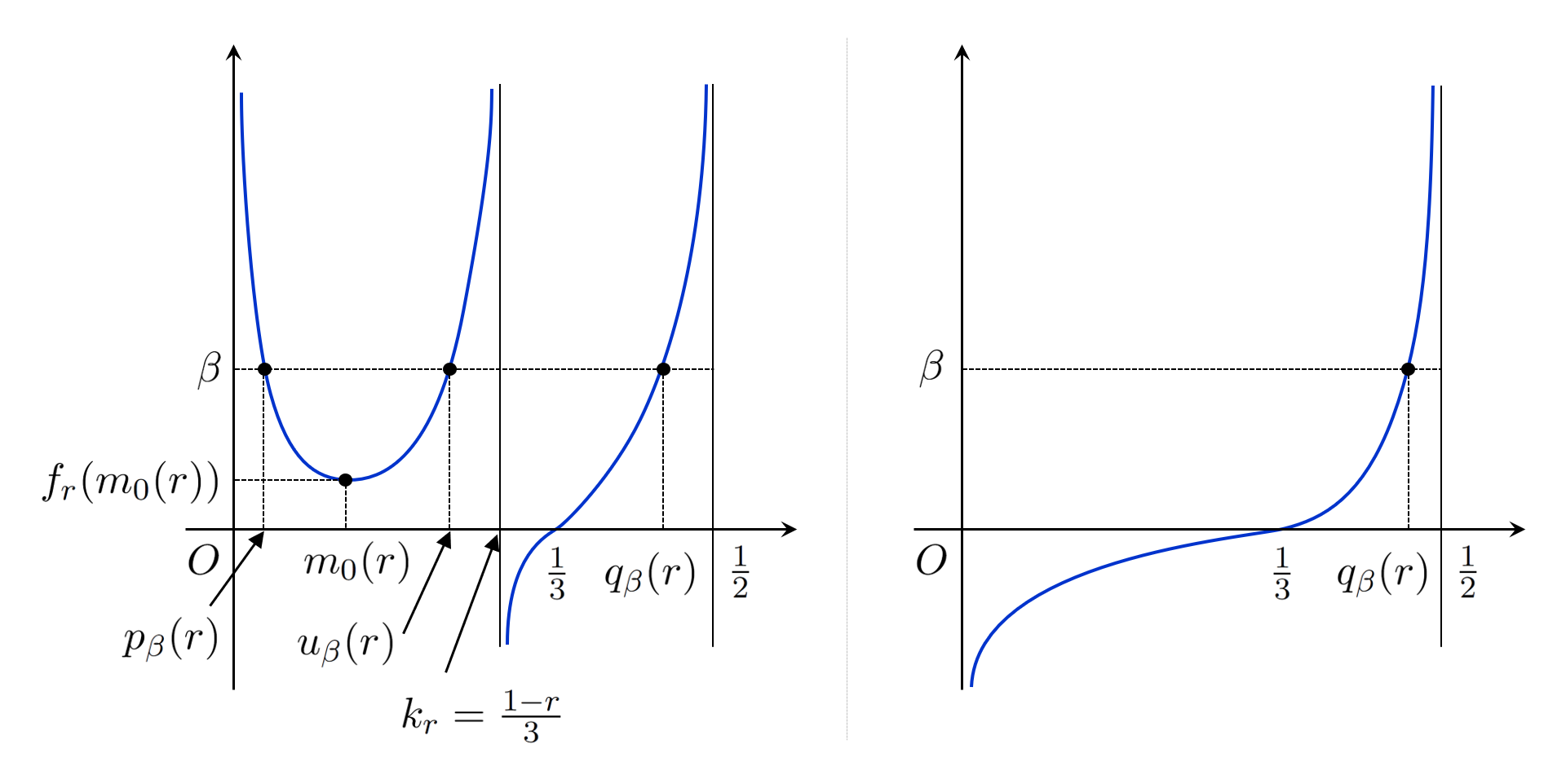
Figure 10. The graph of $f_{r}(\cdot)$ for $r\in(0,1)$ (left) and $r\in[1,\infty)$ (right)

Proof.

It is easy to verify that

$$f_{r}^{\prime}(t)\;=\;\frac{2}{3(1-r-3t)^{2}t(1-2t)}\left[r-h(t)\right]\;,$$

so that (1) is obvious.

We first investigate elementary properties of $h$. Since the derivative of $h$ is given by $h^{\prime}(t)=-3(1-4t)\log((1-2t)/t)$, the function $h(t)$ is decreasing on $(0,\,1/4)\cup(1/3,\,1/2)$ and increasing on $(1/4,\,1/3)$. We refer to Figure 11 for the graph of $h(t)$. Since $\lim_{t\downarrow 0}h(t)=1$ and $h(1/3)=0$, we can verify that the equation $h(t)=r$ has only one solution $m_{0}(r)$ if $0<r<1$ and no solution if $r\geq 1$.

For (2), fix $0<r<1$, and then observe from the graph of $h$ that $h(t)>r$ on $t\in(0,\,m_{0}(r))$ and $h(t)<r$ on $t\in(m_{0}(r),\,1/2)$. We can check from an elementary calculation that $h(k_{r})<r$ and hence $m_{0}(r)<k_{r}$. This completes the proof of the first part of (2). The second part of (2) is direct from (1). The last part of (2) follows easily from an elementary computation.

For (3), since $h(t)<r$ for all $r\geq 1$, the first part is obvious. The remaining part is direct from the expression of $f_{r}(t)$.

Assertion (4) is obvious from the fact that $h(m_{0}(r))=r$ for $0<r<1$. To prove (5), note that $f_{r}(t)$ can be written as

$$f_{r}(t)\;=\;\frac{2}{9}\,\frac{1-h(t)-3t}{(1-r-3t)t(1-2t)}\;\cdot$$

Since $h(m_{0}(r))=r$, this equation becomes

$$f_{r}(m_{0}(r))\;=\;\frac{2}{9m_{0}(r)(1-2m_{0}(r))}\;\cdot$$ (5.5)

By the fact that $m_{0}(r)<m_{0}(0)=m_{0}<1/4$, where $m_{0}$ is defined in Section 4, and that $m_{0}(r)$ is decreasing in $r$, we can check that the right hand side of the previous displayed equation is increasing in $r$. The second assertion of (5) follows from (3). ∎

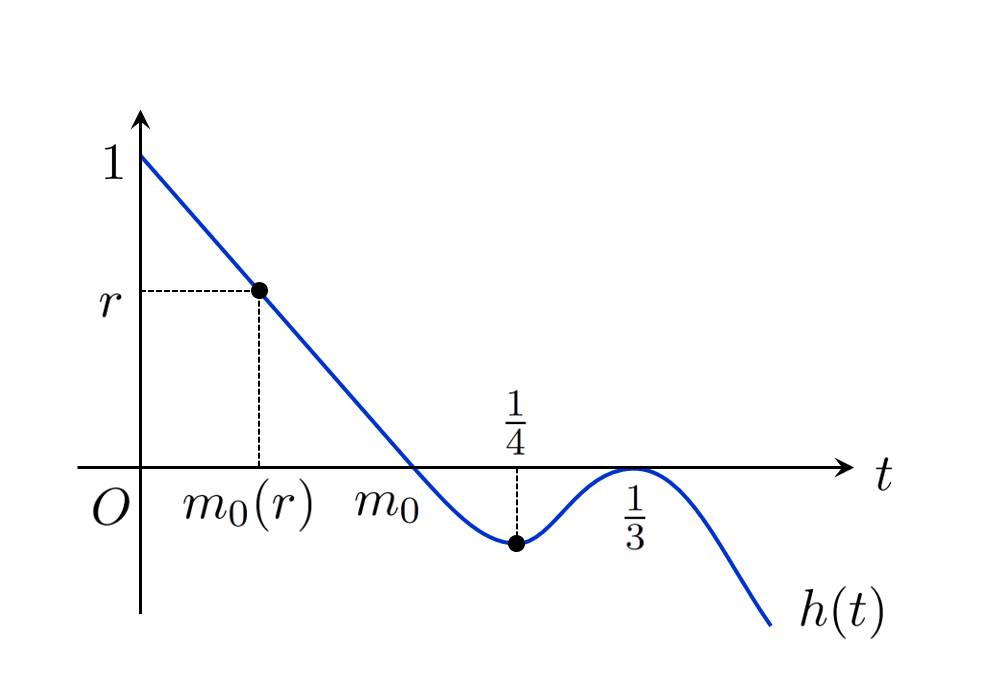
Figure 11. The graph of $h(t)$.

Recall that $f_{0}(m_{0})=\beta_{3}<2$. Hence, by (5) of Lemma 5.3 and the intermediate value theorem, there exists unique $r\in(0,\,1)$ such that $f_{r}(m_{0}(r))=\beta$. Denote such $r$ by $r_{2}^{\beta}$. By (5.5) and the fact that $h(m_{0}(r))=r$, we can obtain the following formula for $r_{2}^{\beta}$:

$$r_{2}^{\beta}\;=\;h\left(\,\frac{1}{4}-\sqrt{\frac{1}{16}-\frac{1}{9\beta}}\,\right)$$ (5.6)

For $r\in(0,\,r_{2}^{\beta})$, the minimum of $f_{r}(t)$ on $(0,\,k_{r})$, which is $f_{r}(m_{0}(r))$, is less than $\beta$. Therefore, for such $r$, the equation $f_{r}(t)=\beta$ has three solutions $p_{\beta}(r)<u_{\beta}(r)<q_{\beta}(r)$ on $(0,\,1/2),$ where

$$p_{\beta}\;\in\;(0,\,m_{0}(r))\;,\;\;u_{\beta}\;\in\;(m_{0}(r),\,k_{r})\;,\;\;q_{\beta}(r)\;\in\;(1/3,\,1/2)\;.$$

We remark that $q_{\beta}(r)$ is larger than $1/3$ since $f_{r}(1/3)=0$ for all $r>0$. On the other hand, for $r\in(r_{2}^{\beta},\,\infty)$, by (3) of Lemma 5.3, there is only one solution for $f_{r}(t)=\beta$ on $(1/3,\,1/2)$ and we denote this again by $q_{\beta}(r)$. We refer to Figure 10 for the visualization.

In conclusion, there are three critical points $\boldsymbol{m}_{0}^{\beta}(r)=(p_{\beta}(r),p_{\beta}(r))$, $\boldsymbol{p}^{\beta}(r)=(u_{\beta}(r),u_{\beta}(r))$, and $\boldsymbol{\sigma}_{0}^{\beta}(r)=(q_{\beta}(r),q_{\beta}(r))$ on the line $\{\boldsymbol{x}:x_{1}=x_{2}\}$ for $r\in(0,\,r_{2}^{\beta})$, while there is only one critical point $\boldsymbol{\sigma}_{0}^{\beta}(r)=(q_{\beta}(r),q_{\beta}(r))$ for $r>r_{2}^{\beta}$. Note that, for small $r$, this notation is in accordance with the one defined in Section 5.1 for small $r$.

In the next lemma we examine the properties of these critical points. Let

$$r_{1}^{\beta}\;=\;1\;-\;\frac{2}{\beta}\;-\;\frac{2}{3\beta}\log\left(\frac{3\beta}{2}-2\right)\;.$$ (5.7)

It is easy to check that $r_{1}^{\beta}<r_{2}^{\beta}$ for all $\beta>2$ since $f_{r_{1}^{\beta}}(m_{0}(r_{1}^{\beta}))<\beta$.

Lemma 5.4.

We have that

1. The point $\boldsymbol{m}_{0}^{\beta}(r)$ is a local minimum of $F_{\beta}(\cdot,r)$ for all $r\in(0,\,r_{2}^{\beta})$;

2. The point $\boldsymbol{\sigma}_{0}^{\beta}(r)$ is a saddle point of $F_{\beta}(\cdot,r)$ for all $r>0$;

3. The point $\boldsymbol{p}^{\beta}(r)$ is a local maxima of $F_{\beta}(\cdot,r)$ for all $r\in(0,\,r_{1}^{\beta})$, and a saddle point of $F_{\beta}(\cdot,r)$ for all $r\in(r_{1}^{\beta},\,r_{2}^{\beta})$.

Proof.

Recall from (3.16) that the determinant and the trace of the Hessian of $F_{\beta}(\cdot,r)$ at the point $(t,\,t)$, $t\in(0,\,1/2)$, are given by

$$(\det\,\nabla^{2}F_{\beta})(t,t,r)\;=\;\left(\frac{1}{\beta t}-\frac{3}{2}\right)\left(\frac{2}{\beta(1-2t)}+\frac{1}{\beta t}-\frac{9}{2}\right)\;,$$ (5.8)

$$\quad(\mbox{tr }\nabla^{2}F_{\beta})(t,t,r)\;=\;\frac{1}{\beta(1-2t)}+\frac{1}{\beta t}-3\;.$$

To prove assertion (1), we claim that

$$\frac{1}{\beta p_{\beta}(r)}-\frac{3}{2}\;>\;0\;\;\mbox{and}\;\;\frac{2}{\beta(1-2p_{\beta}(r))}+\frac{1}{\beta p_{\beta}(r)}-\frac{9}{2}\;>\;0$$ (5.9)

for all $r\in(0,\,r_{2}^{\beta}).$ For the first inequality, substitute $\beta$ by $f_{r}(p_{\beta}(r))$ to rewrite the inequality as

$$\frac{1}{f_{r}(p_{\beta}(r))\,p_{\beta}(r)}-\frac{3}{2}\;>\;0\;.$$

By a straightforward computation, we can show that this inequality is equivalent to $k(p_{\beta}(r))<1-r$ where

$$k(t)\;=\;3t\;+\;t\log\frac{1-2t}{t}\;\cdot$$

Since $k^{\prime}(t)>0$ for $t\in(0,\,m_{0})$, we have that $k(p_{\beta}(r))<k(m_{0}(r))$. As $m_{0}(r)$ satisfies $f_{r}^{\prime}(m_{0}(r))=0$, i.e.,

$$\log\frac{1-2m_{0}(r)}{m_{0}(r)}\;=\;\frac{1-r-3m_{0}(r)}{3m_{0}(r)(1-2m_{0}(r))}\;,$$

we obtain that

$$k(m_{0}(r))\;=\;3m_{0}(r)+\frac{1-r-3m_{0}(r)}{3(1-2m_{0}(r))}\;.$$

Since $m_{0}(r)<k_{r}=(1-r)/3$, the inequality $k(m_{0}(r))<1-r$ is equivalent to $3(1-2m_{0}(r))>1$. Since $1-2m_{0}(r)>1-2m_{0}>1/3$, we obtain $k(m_{0}(r))<1-r$, and thus $k(p_{\beta}(r))<1-r$. This proves the first inequality of (5.9). For the second inequality, by replacing $\beta$ by $f_{r}(p_{\beta}(r))$, we can reorganize the inequality as $h(p_{\beta}(r))>r$. This is true by (1), (2) of Lemma 5.3 because $p_{\beta}(r)\in(0,\,m_{0}(r))$. This completes the proof of (5.9).

By (5.8) and (5.9), the Hessian of $F_{\beta}(\cdot,r)$ at $\boldsymbol{m}_{0}^{\beta}(r)$ is positive definite, which proves assertion (1) of the Lemma.

We turn to (2). To prove that the Hessian of $F_{\beta}(\cdot,r)$ at $\boldsymbol{\sigma}_{0}^{\beta}(r)$ is negative definite, it suffices to show that

$$\frac{1}{\beta q_{\beta}(r)}-\frac{3}{2}\;<\;0\;\;\mbox{and}\;\;\frac{2}{\beta(1-2q_{\beta}(r))}+\frac{1}{\beta q_{\beta}(r)}-\frac{9}{2}\;>\;0$$ (5.10)

for all $r>0$. The first inequality is obvious since $\beta>2$ and $q_{\beta}(r)>1/3$. For the second inequality, by the same type of substitution performed in the proof of assertion (1), we can reduce the inequality to $h(q_{\beta}(r))<r$, which follows from the proof of Lemma 5.3, where we proved that $h(t)<0$ for $t>1/3$.

It remains to prove assertion (3). As in the first part of the proof, we can show that

$$\frac{2}{\beta(1-2u_{\beta}(r))}\;+\;\frac{1}{\beta u_{\beta}(r)}-\frac{9}{2}\;<\;0$$ (5.11)

for all $r\in(0,\,r_{2}^{\beta})$.

We claim that $u_{\beta}(r)$ is decreasing in $r$. By differentiating $f_{r}(u_{\beta}(r))=\beta$ in $r$, we obtain that

$$\frac{2}{3(1-r-3u_{\beta}(r))^{2}}\left[(-1-3u_{\beta}^{\prime}(r))\log\frac{1-2u_{\beta}(r)}{u_{\beta}(r)}+\frac{u_{\beta}^{\prime}(r)(1-r-3u_{\beta}(r))}{u_{\beta}(r)(1-2u_{\beta}(r))}\right]\;=\;0\;.$$

Since $f_{r}(u_{\beta}(r))=\beta$, replace $\log\left[(1-2u_{\beta}(r))/u_{\beta}(r)\right]$ by $\frac{3}{2}(1-r-3u_{\beta}(r))\beta$, and reorganize the previous equality as

$$u_{\beta}^{\prime}(r)\left[\frac{1}{u_{\beta}(r)(1-2u_{\beta}(r))}-\frac{9}{2}\beta\right]\;=\;\frac{3}{2}\beta\;.$$

By (5.11), the expression inside of the bracket is negative so that $u_{\beta}(r)$ is decreasing in $r$.

By the definition (5.7) of $r_{1}^{\beta}$ and a direct calculation, $f_{r_{1}^{\beta}}\big{(}2/(3\beta)\big{)}=\beta$. Since $2/(3\beta)<1/3$, $2/(3\beta)$ is either $p_{\beta}(r_{1}^{\beta})$ or $u_{\beta}(r_{1}^{\beta})$. An elementary computation shows that $h(2/(3\beta))<r_{1}^{\beta}$ so that $2/(3\beta)=u_{\beta}(r_{1}^{\beta})$. Since $u_{\beta}(r)$ is decreasing,

$$\frac{1}{\beta u_{\beta}(r)}\;<\;\frac{3}{2}\mbox{\;\;for\;\;}r\;\in\;(0,\,r_{1}^{\beta})\;\;\mbox{and\;\;}\frac{1}{\beta u_{\beta}(r)}\;>\;\frac{3}{2}\mbox{\;\;for\;\;}r\;\in\;(r_{1}^{\beta},\,r_{2}^{\beta})\;.$$ (5.12)

At this point, by combining these results and (5.11), the proofs of the assertions (3) for $r\in(0,\,r_{1}^{\beta})$ and $r\in(r_{1}^{\beta},\,r_{2}^{\beta})$ are essentially same to those of (1) and (2), respectively. ∎

Remark 5.5.

The point $\boldsymbol{p}^{\beta}(r)$ is a degenerate critical point of $F_{\beta}(\cdot,r)$ if $r=r_{1}^{\beta}$.

B. Critical points not on the line $\{{\boldsymbol{x}}:x_{1}=x_{2}\}$. We now consider the critical points which are not on the line $\{{\boldsymbol{x}}:x_{1}=x_{2}\}$. Let $G_{\beta}:(0,\,\infty)\to{\mathbb{R}}$ be the function given by $G_{\beta}(x)=(1/\beta)\log x-(3x/2)$. With this notation we can rewrite (5.4) as

$$G_{\beta}(x_{0})+3r/2\;=\;G_{\beta}(x_{1})=G_{\beta}(x_{2})\;.$$ (5.13)

Let $l_{\beta}:=2/(3\beta)$, $g_{\beta}:=G_{\beta}(l_{\beta})$. It is easy to verify that $G_{\beta}$ is increasing on $(0,\,l_{\beta})$, decreasing on $(l_{\beta},\,\infty)$, and that $\lim_{x\downarrow 0}G_{\beta}(x)=\lim_{x\uparrow\infty}G_{\beta}(x)=-\infty$. Hence, for all $y\in(-\infty,\,g_{\beta})$, there are two solutions $H_{\beta}(y)<l_{\beta}<K_{\beta}(y)$ of the equation $G_{\beta}(x)=y$. Let $H_{\beta}(g_{\beta})=K_{\beta}(g_{\beta})=l_{\beta}$, and note that $H_{\beta}$ and $K_{\beta}$ are continuous increasing and decreasing functions on $(-\infty,\,g_{\beta}]$, respectively. We refer to Figure 12.

Figure 12. The graph of $G_{\beta}$ and the definitions of $H_{\beta}$, $K_{\beta}$.

Lemma 5.6.

Let $S_{\beta}^{(k)}:(-\infty,g_{\beta}]\to{\mathbb{R}}$, $k=1,\,2$, be the function given by $S_{\beta}^{(k)}(y)=kH_{\beta}(y)+K_{\beta}(y)$. Then,

1. The function $S_{\beta}^{(1)}$ is decreasing on $(-\infty,\,g_{\beta}]$;

2. There exists $\tilde{g}_{\beta}<g_{\beta}$ such that $S_{\beta}^{(2)}$ is decreasing on $(-\infty,\,\tilde{g}_{\beta})$ and increasing on $(\tilde{g}_{\beta},\,g_{\beta}]$.

Proof.

Since we can regard $H_{\beta}$ and $K_{\beta}$ as inverses of $G_{\beta}$, their derivatives at $y<g_{\beta}$ can be written as

$$H_{\beta}^{\prime}(y)\;=\;\beta\left[\frac{1}{H_{\beta}(y)}\,-\,\frac{1}{l_{\beta}}\right]^{-1}\;\;\mbox{and}\;\;\;K_{\beta}^{\prime}(y)\;=\;\beta\left[\frac{1}{K_{\beta}(y)}\,-\,\frac{1}{l_{\beta}}\right]^{-1}\;.$$ (5.14)

Since $H_{\beta}(y)<l_{\beta}<K_{\beta}(y)$ for $y<g_{\beta}$, the inequality $H_{\beta}^{\prime}(y)+K_{\beta}^{\prime}(y)\leq 0$ is satisfied if

$$\frac{2}{l_{\beta}}-\frac{1}{H_{\beta}(y)}\,-\,\frac{1}{K_{\beta}(y)}\;\leq\;0\;\;\text{or, equivalently,}\;\left[\frac{2}{l_{\beta}}-\frac{1}{K_{\beta}(y)}\right]^{-1}\;\geq\;H_{\beta}(y)\;.$$ (5.15)

Since the left hand side of the last inequality is less than $l_{\beta},$ since $G_{\beta}$ is increasing on $(0,l_{\beta})$, and since $G_{\beta}(K_{\beta}(y))=G_{\beta}(H_{\beta}(y))$, this inequality is equivalent to $L_{\beta}^{(1)}\big{(}K_{\beta}(y)\big{)}\geq 0$ where

$$L_{\beta}^{(1)}(t)\;=\;G_{\beta}\left(\left[\frac{2}{l_{\beta}}-\frac{1}{t}\right]^{-1}\right)\,-\,G_{\beta}(t)\;,\;\;t\geq l_{\beta}\;.$$

It is easy to see that $L_{\beta}^{(1)}$ is increasing so that $L_{\beta}^{(1)}(t)\geq L_{\beta}^{(1)}(l_{\beta})=0$. This proves assertion (1) of the lemma.

The proof of assertion (2) is analogous. By the arguments presented above, the sign of the function $2H_{\beta}^{\prime}(y)+K_{\beta}^{\prime}(y)$, $y\leq g_{\beta}$, is the opposite sign of $L_{\beta}^{(2)}\big{(}K_{\beta}(y)\big{)}$, where

$$L_{\beta}^{(2)}(t)\;=\;G_{\beta}\left(\left[\frac{3}{l_{\beta}}\,-\,\frac{2}{t}\right]^{-1}\right)-G_{\beta}(t)\;,\;\;t\;\geq\;l_{\beta}\;.$$

A direct computation shows that $L_{\beta}^{(2)}(t)$ is increasing on $(l_{\beta},\,4l_{\beta}/3)$ and decreasing on $(4l_{\beta}/3,\,\infty)$. Since $L_{\beta}^{(2)}(l_{\beta})=0$ and $\lim_{t\rightarrow\infty}L_{\beta}^{(2)}(t)=-\infty$, we can conclude the proof of assertion (2). ∎

By (5.13), a critical point $\boldsymbol{x}=(x_{1},x_{2})$ such that $x_{1}\neq x_{2}$ satisfies $(x_{1},x_{2})=\big{(}H_{\beta}(y),K_{\beta}(y)\big{)}$ or $(x_{1},x_{2})=\big{(}K_{\beta}(y),H_{\beta}(y)\big{)}$ for some $y<G_{\beta}(l_{\beta})$. By symmetry, we only consider the first case. There are two possibilities for $x_{0}$ in this situation, namely, $x_{0}=K_{\beta}(y-3r/2)$ or $x_{0}=H_{\beta}(y-3r/2)$. We start by considering the first case.

Lemma 5.7.

The equation

$$K_{\beta}(y-3r/2)+H_{\beta}(y)+K_{\beta}(y)\;=\;1$$ (5.16)

has a unique solution $y_{1}^{\beta}(r)$ if $r\leq r_{1}^{\beta}$ and has no solution if $r>r_{1}^{\beta}$. Furthermore, $\big{(}H_{\beta}(y_{1}^{\beta}(r)),\,K_{\beta}(y_{1}^{\beta}(r))\big{)}$ is a saddle point of $F_{\beta}(\cdot,r)$ if $r<r_{1}^{\beta}$.

Proof.

Denote by $R_{\beta}^{(1)}(y)$ the left hand side of (5.16). By (1) of Lemma 5.6, and by the fact that $K_{\beta}$ is strictly decreasing, the function $R_{\beta}^{(1)}$ is a continuous strictly decreasing function on $(-\infty,\,g_{\beta})$. Since $\lim_{y\rightarrow-\infty}R_{\beta}^{(1)}(y)=\infty$, the solution of (5.16) does uniquely exist if $R_{\beta}^{(1)}(g_{\beta})\geq 1$, and does not exist if $R_{\beta}^{(1)}(g_{\beta})<1$. Since $H_{\beta}(g_{\beta})=K_{\beta}(g_{\beta})=l_{\beta}$, by an elementary computation we can check that $R_{\beta}^{(1)}(g_{\beta})\geq 1$ if $r\leq r_{1}^{\beta}$, and $R_{\beta}^{(1)}(g_{\beta})<1$ if $r>r_{1}^{\beta}$. This proves the first part of lemma.

For the second part, it suffices to show that $(\nabla^{2}F_{\beta})(H_{\beta}(y),K_{\beta}(y),r)$, $y\leq g_{\beta}$, has a negative determinant for all $r\leq r_{1}^{\beta}$. Let

$$a_{0}(y)\;=\;\frac{1}{\beta K_{\beta}(y-3r/2)}-\frac{3}{2}\;,\;\;a_{1}(y)\;=\;\frac{1}{\beta H_{\beta}(y)}-\frac{3}{2}\;,\;\;a_{2}(y)\;=\;\frac{1}{\beta K_{\beta}(y)}-\frac{3}{2}\;\cdot$$

Then, by (3.16), we can write

$$\det\big{[}(\nabla^{2}F_{\beta})(H_{\beta}(y),K_{\beta}(y),r)\big{]}\;=\;a_{0}(y)a_{1}(y)a_{2}(y)\left[\frac{1}{a_{0}(y)}+\frac{1}{a_{1}(y)}+\frac{1}{a_{2}(y)}\right]\;.$$

Observe that $a_{0}(y),\,a_{2}(y)<0$, $a_{1}(y)>0$ and, by (5.14),

$$\frac{1}{a_{0}(y)}+\frac{1}{a_{1}(y)}+\frac{1}{a_{2}(y)}\;=\;\frac{dR_{\beta}^{(1)}}{dy}(y)\;<\;0\;.$$

These observations prove that the right hand side of the penultimate displayed equation is negative, as claimed. ∎

We turn to the second case.

Lemma 5.8.

For all $r>0$, the equation

$$H_{\beta}(y-3r/2)+H_{\beta}(y)+K_{\beta}(y)\;=\;1$$ (5.17)

has unique solution $y_{2}^{\beta}(r)$. Furthermore, the point $\big{(}H_{\beta}(y_{2}^{\beta}(r)),\,K_{\beta}(y_{2}^{\beta}(r))\big{)}$ is a local minimum of $F_{\beta}(\cdot,r)$.

Proof.

Denote by $R_{\beta}^{(2)}(y)$ the left hand side of (5.17). By the fact that $H_{\beta}$ is increasing, and by (5.14), we have that

$$R_{\beta}^{(2)}(y)\;<\;S_{\beta}^{(2)}(y)\;\;\text{and}\;\;\frac{dR_{\beta}^{(2)}}{dy}(y)\;<\;\frac{dS_{\beta}^{(2)}}{dy}(y)\;\;\mbox{for all }y\;\in\;(-\infty,\,g_{\beta}]\;.$$ (5.18)

Furthermore,

$$\lim_{y\rightarrow-\infty}R_{\beta}^{(2)}(y)\;=\;\infty\;\;\mbox{and}\;\;R_{\beta}^{(2)}(g_{\beta})\;<\;S_{\beta}^{(2)}(g_{\beta})\;=\;3l_{\beta}\;=\;2/\beta\;<\;1\;,$$

the equation $R_{\beta}^{(2)}(y)=1$ has at least one solution. By the first inequality of (5.2), by (2) of Lemma 5.6, and by the fact that $S_{\beta}^{(2)}(g_{\beta})<1$, the solution of $R_{\beta}^{(2)}(y)=1$ should be less than $\tilde{g}_{\beta}$. By the second inequality of (5.2) and by (2) of Lemma 5.6, $R_{\beta}^{(2)}$ is strictly decreasing on $(-\infty,\,\tilde{g}_{\beta})$. Hence, the solution of the equation $R_{\beta}^{(2)}(y)=1$ is unique.

We now prove that the Hessian of $F_{\beta}(\cdot,r)$ at $(H_{\beta}(y),\,K_{\beta}(y))$ is positive definite for all $y<\tilde{g}_{\beta}$. Let

$$b_{0}(y)\;=\;\frac{1}{\beta H_{\beta}(y-3r/2)}-\frac{3}{2}\;,\;\;b_{1}(y)\;=\;\frac{1}{\beta H_{\beta}(y)}-\frac{3}{2}\;,\;\;b_{2}(y)\;=\;\frac{1}{\beta K_{\beta}(y)}-\frac{3}{2}\;.$$

The positiveness of $\det\big{[}(\nabla^{2}F_{\beta})(H_{\beta}(y),\,K_{\beta}(y),\,r)\big{]}$ can be proven as in the proof of Lemma 5.7. The trace of the Hessian, which can be written as $2b_{0}(y)+b_{1}(y)+b_{2}(y)$, is positive since $b_{0}(y)>0$ and $b_{1}(y)+b_{2}(y)>0$, where the latter inequality follows from (5.15). ∎

For $r\in(0,\,r_{1}^{\beta})$, by Lemmata 5.7 and 5.8, we obtain four additional critical points on $\{\boldsymbol{x}:x_{1}\neq x_{2}\}$

$$\boldsymbol{\sigma}_{1}^{\beta}(r)\;=\;\big{(}K_{\beta}(y_{1}^{\beta}(r)),\,H_{\beta}(y_{1}^{\beta}(r))\big{)}\;,\;\;\boldsymbol{\sigma}_{2}^{\beta}(r)\;=\;\big{(}H_{\beta}(y_{1}^{\beta}(r)),\,K_{\beta}(y_{1}^{\beta}(r))\big{)}\;,\;\;$$

$$\quad\boldsymbol{m}_{1}^{\beta}(r)\;=\;\big{(}H_{\beta}(y_{2}^{\beta}(r)),\,K_{\beta}(y_{2}^{\beta}(r))\big{)}\;,\;\;\boldsymbol{m}_{2}^{\beta}(r)\;=\;\big{(}K_{\beta}(y_{2}^{\beta}(r)),\,H_{\beta}(y_{2}^{\beta}(r))\big{)}\;.$$

One can easily verify that this notation coincides with the one adopted in Section 5.1 for small $r$. On the other hand, for $r\in(r_{1}^{\beta},\,\infty)$, there are only two critical points $\boldsymbol{m}_{1}^{\beta}(r),\,\boldsymbol{m}_{2}^{\beta}(r)$ on $\{\boldsymbol{x}:x_{1}\neq x_{2}\}$ which are local minima of $F_{\beta}(\cdot,r)$.

C. The structure of the valleys. We first compare the heights of the local minima of $F_{\beta}(\cdot,\,r)$. For $r>r_{2}^{\beta}$, there are two local minima $\boldsymbol{m}_{1}^{\beta}(r)$ and $\boldsymbol{m}_{1}^{\beta}(r)$, and it is obvious from the symmetry that

$$F_{\beta}(\boldsymbol{m}_{1}^{\beta}(r),r)\;=\;F_{\beta}(\boldsymbol{m}_{2}^{\beta}(r),r);.$$

Hence, it suffices to focus only on the case $r<r_{2}^{\beta}$.

Lemma 5.9.

For $r\in(0,\,r_{2}^{\beta})$, the three local minima of $F_{\beta}(\cdot,r)$ satisfy

$$F_{\beta}(\boldsymbol{m}_{1}^{\beta}(r),r)\;=\;F_{\beta}(\boldsymbol{m}_{2}^{\beta}(r),r)\;<\;F_{\beta}(\boldsymbol{m}_{0}^{\beta}(r),r)\;.$$

In particular, $\boldsymbol{m}_{1}^{\beta}(r)$ and $\boldsymbol{m}_{2}^{\beta}(r)$ are the global minima of $F_{\beta}(\cdot,r)$ for all $r>0$.

Proof.

Since $\boldsymbol{m}_{i}^{\beta}(0)=\boldsymbol{m}_{i}^{\beta}$, the three values $F_{\beta}(\boldsymbol{m}_{i}^{\beta}(0),0)$, $0\leq i\leq 2$, are the same. Hence, it suffices to prove that

$$\frac{d}{dr}F_{\beta}(\boldsymbol{m}_{0}^{\beta}(r),r)\;>\;0\;\;\mbox{and}\;\;\frac{d}{dr}F_{\beta}(\boldsymbol{m}_{1}^{\beta}(r),r)\;=\;\frac{d}{dr}F_{\beta}(\boldsymbol{m}_{2}^{\beta}(r),r)\;<\;0\;.$$ (5.19)

By the chain rule, and by the fact that $\boldsymbol{m}_{i}^{\beta}(r)$, $0\leq i\leq 2$, are critical points of $F_{\beta}(\cdot,r)$, it is easy to check that

$$\frac{d}{dr}F_{\beta}(\boldsymbol{m}_{0}^{\beta}(r),r)\;=\;1-3p_{\beta}(r)$$

$$\frac{d}{dr}F_{\beta}(\boldsymbol{m}_{i}^{\beta}(r),r)\;=\;H_{\beta}\big{(}y_{1}^{\beta}(r)-3r/2\big{)}\;-\;\frac{H_{\beta}(y_{1}^{\beta}(r))+K_{\beta}(y_{1}^{\beta}(r))}{2}\;,\;i=1,\,2\;.$$

Assertion (5.19) follows from the fact that $p_{\beta}(r)<1/3$ and $H_{\beta}\big{(}y_{1}^{\beta}(r)-3r/2\big{)}<H_{\beta}(y_{1}^{\beta}(r))<K_{\beta}(y_{1}^{\beta}(r))$. ∎

To compare the heights of saddle points, let

$$h_{0}^{\beta}(r)\;=\;F_{\beta}(\boldsymbol{\sigma}_{0}^{\beta}(r),r)\;\;\mbox{and}\;\;h_{1}^{\beta}(r)\;=\;\begin{cases}F_{\beta}(\boldsymbol{\sigma}_{1}^{\beta}(r),r)&\mbox{if }r\in(0,\,r_{1}^{\beta})\;,\\ F_{\beta}(\boldsymbol{p}^{\beta}(r),r)&\mbox{if }r\in(r_{1}^{\beta},\,r_{2}^{\beta})\;.\end{cases}$$

Lemma 5.10.

For $r\in(0,\,r_{1}^{\beta})\cup(r_{1}^{\beta},\,r_{2}^{\beta})$, we have that $h_{0}^{\beta}(r)<h_{1}^{\beta}(r)$.

Proof.

An argument, analogous to the one presented in the proof of Lemma 5.9, proves the assertion of the lemma for $r\in(0,\,r_{1}^{\beta})$. For $r\in(r_{1}^{\beta},\,r_{2}^{\beta})$, one can check that the function $t\mapsto F_{\beta}(t,t,r)$ is decreasing on $(u_{\beta}(r),q_{\beta}(r))$. The assertion of the lemma follows automatically. ∎

To complete the description of the metastable behavior, we investigate the structure of the valleys for each value of $r$. We start with an elementary observation.

Lemma 5.11.

For $r\in(0,\,r_{1}^{\beta})\cup(r_{1}^{\beta},\,r_{2}^{\beta})$, define the line $\boldsymbol{l}_{\beta}(r)$ as

$$\boldsymbol{l}_{\beta}(r)\;=\;\begin{cases}\{\boldsymbol{x}:x_{1}+x_{2}=H_{\beta}(y_{1}^{\beta}(r))+K_{\beta}(y_{1}^{\beta}(r))\}\cap\Xi&\mbox{if }r\in(0,\,r_{1}^{\beta})\\ \{\boldsymbol{x}:x_{1}+x_{2}=2u_{\beta}(r)\}\cap\Xi&\mbox{if }r\in(r_{1}^{\beta},\,r_{2}^{\beta})\end{cases}$$

Then, $F_{\beta}(\cdot,r)$ restricted to $\boldsymbol{l}_{\beta}(r)$ achieves its minimum only at $\boldsymbol{\sigma}_{1}^{\beta}(r)$ and $\boldsymbol{\sigma}_{2}^{\beta}(r)$ if $r\in(0,\,r_{1}^{\beta})$, and at $\boldsymbol{p}^{\beta}(r)$ if $r\in(r_{1}^{\beta},\,r_{2}^{\beta})$.

Proof.

For the first part, it can be shown by a simple differentiation that the function

$$t\;\mapsto\;F_{\beta}(t,\,H_{\beta}(y_{1}^{\beta}(r))+K_{\beta}(y_{1}^{\beta}(r))-t,\,r)$$

achieves a minimum only at $t=H_{\beta}(y_{1}^{\beta}(r))$ and $t=K_{\beta}(y_{1}^{\beta}(r))$. The proof of the second assertion is similar. ∎

Next lemma describes the structure of the valleys at heights $h_{0}^{\beta}(r)$ and $h_{1}^{\beta}(r)$.

Lemma 5.12.

For all $r>0$, the set $\{\boldsymbol{x}\in\Xi:F_{\beta}(\boldsymbol{x},r)<h_{0}^{\beta}(r)\}$ has two connected components, denoted by $W_{\beta}(1,r)$ and $W_{\beta}(2,r)$, such that $\boldsymbol{m}_{i}^{\beta}(r)\in W_{\beta}(i,r)$, $i=1,\,2$, and $\overline{W_{\beta}(1,r)}\cap\overline{W_{\beta}(2,r)}=\{\boldsymbol{\sigma}_{0}^{\beta}(r)\}$. For small enough $r$, there is an additional component, represented by $W_{\beta}(0,r)$, containing $\boldsymbol{m}_{0}^{\beta}$ and satisfying $\overline{W_{\beta}(0,r)}\cap\overline{W_{\beta}(i,r)}=\varnothing$ for $i=1,\,2$.

Proof.

It is obvious that the set $\{\boldsymbol{x}\in\Xi:F_{\beta}(\boldsymbol{x},r)<h_{0}^{\beta}(r)\}$ is composed of two connected components, denoted by $W_{\beta}(1,r)$ and $W_{\beta}(2,r)$, such that $\boldsymbol{m}_{i}^{\beta}(r)\in W_{\beta}(i,r)$, $i=1,\,2$.

By combining the fact that $F_{\beta}(\boldsymbol{m}_{0}^{\beta}(0),\,0)<F_{\beta}(\boldsymbol{\sigma}_{0}^{\beta}(0),\,0)$, $F_{\beta}(\boldsymbol{m}_{0}^{\beta}(r_{2}^{\beta}),\,r_{2}^{\beta})>F_{\beta}(\boldsymbol{\sigma}_{0}^{\beta}(r_{2}^{\beta}),\,r_{2}^{\beta})$ and that the map $r\mapsto F_{\beta}(\boldsymbol{m}_{0}^{\beta}(r),\,r)-F_{\beta}(\boldsymbol{\sigma}_{0}^{\beta}(r),\,r)$ is increasing, as shown in the proof of Lemmata 5.9, 5.10, we can assert that there exists $r_{*}^{\beta}<r_{2}^{\beta}$ such that

$$\begin{cases}F_{\beta}(\boldsymbol{m}_{0}^{\beta}(r),\,r)\;<\;F_{\beta}(\boldsymbol{\sigma}_{0}^{\beta}(r),\,r)&\mbox{if }r<r_{*}^{\beta}\;,\\ F_{\beta}(\boldsymbol{m}_{0}^{\beta}(r),\,r)\;\geq\;F_{\beta}(\boldsymbol{\sigma}_{0}^{\beta}(r),\,r)&\mbox{if }r\geq r_{*}^{\beta}\;.\end{cases}$$

Hence, for $r<r_{*}^{\beta}$, we have an additional connected component, denoted by $W_{\beta}(0,r)$, containing $\boldsymbol{m}_{0}^{\beta}(r)$, while this component disappears for $r\geq r_{*}^{\beta}$. Since, for $r<r_{2}^{\beta}$, $\boldsymbol{m}_{0}^{\beta}(r)$ and $\{\boldsymbol{m}_{1}^{\beta}(r),\,\boldsymbol{m}_{2}^{\beta}(r)\}$ are on the different sides of the line $\boldsymbol{l}_{\beta}(r)$, and since, by Lemmata 5.10, 5.11, $F_{\beta}(\cdot,r)>h_{0}^{\beta}(r)$ on the line $\boldsymbol{l}_{\beta}(r)$, the component $W_{\beta}(0,r)$ is isolated from the other components. Therefore, it is enough to show that $\overline{W_{\beta}(1,r)}\cap\overline{W_{\beta}(2,r)}=\{\boldsymbol{\sigma}_{0}^{\beta}(r)\}$ for all $r>0$. The proof of this fact is analogous to the one of assertion (2) of Proposition 4.4. The details are left to the reader. ∎

Lemma 5.13.

For $r\in(0,\,r_{1}^{\beta})\cup(r_{1}^{\beta},\,r_{2}^{\beta})$, the set $\{\boldsymbol{x}\in\Xi:F_{\beta}(\boldsymbol{x},r)<h_{1}^{\beta}(r)\}$ consists of two connected components, denoted by $V_{\beta}(0,r)$ and $V_{\beta}(1,r)$, such that $\boldsymbol{m}_{0}^{\beta}(r)\in V_{\beta}(0,r)$ and $\boldsymbol{m}_{1}^{\beta}(r),\,\boldsymbol{m}_{2}^{\beta}(r)\in V_{\beta}(1,r)$. The set $\overline{V_{\beta}(0,r)}\cap\overline{V_{\beta}(1,r)}$ is equal to $\{\boldsymbol{\sigma}_{1}^{\beta}(r),\,\boldsymbol{\sigma}_{2}^{\beta}(r)\}$ for $r\in(0,\,r_{1}^{\beta})$, and is equal to $\{\boldsymbol{p}^{\beta}(r)\}$ for $r\in(r_{1}^{\beta},\,r_{2}^{\beta})$.

Proof.

We first consider the case $r\in(0,\,r_{1}^{\beta})$. By Lemma 5.12, there exist two paths $\boldsymbol{\gamma}_{i}^{\beta}(r)$, $i=1,\,2$, connecting $\boldsymbol{\sigma}_{0}^{\beta}(r)$ to $\boldsymbol{m}_{i}^{\beta}(r)$ and satisfying $F_{\beta}(\boldsymbol{x},r)\leq F_{\beta}(\boldsymbol{\sigma}_{0}^{\beta}(r),r)$ for all $\boldsymbol{x}\in\boldsymbol{\gamma}_{i}^{\beta}(r)$. By concatenating these two paths $\boldsymbol{\gamma}_{1}^{\beta}(r)$ and $\boldsymbol{\gamma}_{2}^{\beta}(r)$, we can prove that $\boldsymbol{m}_{1}^{\beta}(r)$ and $\boldsymbol{m}_{2}^{\beta}(r)$ are in the same connected component $V_{\beta}(1,r)$ of the set $\{\boldsymbol{x}\in\Xi:F_{\beta}(\boldsymbol{x},r)<h_{1}^{\beta}(r)\}$. Let $V_{\beta}(0,r)$ be the other component containing $\boldsymbol{m}_{0}^{\beta}(r)$. It suffices to show that $\overline{V_{\beta}(0,r)}\cap\overline{V_{\beta}(1,r)}=\{\boldsymbol{\sigma}_{1}^{\beta}(r),\,\boldsymbol{\sigma}_{2}^{\beta}(r)\}$. By assertion (1) of Lemma 5.11, the first set is a subset of the second one. It remains to prove the other inclusion.

By an argument, similar to the one presented in the proof of assertion (2) of Proposition 4.4, we can construct a path $\boldsymbol{\delta}_{1}^{\beta}(r)$, connecting $\boldsymbol{\sigma}_{1}^{\beta}(r)$ and $\boldsymbol{m}_{0}^{\beta}(r)$ and satisfying $F_{\beta}(\boldsymbol{x},r)\leq F_{\beta}(\boldsymbol{\sigma}_{1}^{\beta}(r),r)$ for all $\boldsymbol{x}\in\boldsymbol{\delta}_{1}^{\beta}(r)$, and another path $\boldsymbol{\delta}_{2}^{\beta}(r)$ connecting $\boldsymbol{\sigma}_{1}^{\beta}(r)$ and one of the points $\boldsymbol{m}_{1}^{\beta}(r)$ and $\boldsymbol{m}_{2}^{\beta}(r)$ and satisfying $F_{\beta}(\boldsymbol{x},r)\leq F_{\beta}(\boldsymbol{\sigma}_{1}^{\beta}(r),r)$ for all $\boldsymbol{x}\in\boldsymbol{\delta}_{2}^{\beta}(r)$. This proves that $\boldsymbol{\sigma}_{1}^{\beta}(r)\in\overline{V_{\beta}(0,r)}\cap\overline{V_{\beta}(1,r)}$. By symmetry, $\boldsymbol{\sigma}_{2}^{\beta}(r)$ is also an element of the same set and the proof for $r\in(0,\,r_{1}^{\beta})$ is completed. The proof in the case $r\in(r_{1}^{\beta},r_{2}^{\beta})$ is similar and left to the reader. ∎

The complete description of the metastable behavior of the random walk ${\boldsymbol{r}}_{N}(t)$ in the case $\beta>2$, $\theta_{\text{e}}=\pi$ and $r>0$, $r\not=r^{\beta}_{1}$, can be obtained from Lemmata 5.12 and 5.13 and the results presented in [14].

5.3. General external field with $\theta_{\text{e}}=2k\pi/3$

By an analogue computation to the one presented in the previous subsection, we can rigorously analyze the case $\theta_{\text{e}}=2k\pi/3$, $k=0,\,1,\,2$, and $\beta>2$. We do not repeat the argument here and we only state the main result.

Assume without loss of generality that $k=0$. There exists a critical value $r^{\beta}$, whose closed form is given by

$$r^{\beta}\;=\;h\left(\,\frac{1}{4}+\sqrt{\frac{1}{16}-\frac{1}{9\beta}}\,\right)\;,$$

where $h$ is the function defined in Lemma 5.3, such that

1. For $r\in(0,\,r^{\beta})$, we observe the phenomenon described in case I of Subsection 5.1.

2. For $r\in(r^{\beta},\,\infty)$, there is only one critical point ${\boldsymbol{m}}_{0}^{\beta}(r)$, which is the global minimum. This regime is illustrated by the left graph of Figure 7.

The regime (II) is clearly different from the high temperature regime $\beta<\beta_{3}$ with zero external field in which the entropy prevails. In the present situation, the spins of the configurations corresponding to the unique global minimum are highly concentrated on one spin ${\boldsymbol{v}}_{0}$, while in the high temperature regime with no external field the spins are equally distributed among the three possible values.

We conclude this subsection explaining why there is no intermediate regime. In the case $\theta_{\text{e}}=0$, for instance, the study of critical points on the line $\{{\boldsymbol{x}}:x_{1}=x_{2}\}$ is related to the solution of $\tilde{f}_{r}(t)=\beta$ where

$$\tilde{f}_{r}(t)\;=\;\frac{2}{3(1+r-3t)}\log{\frac{1-2t}{t}}\;.$$

Notice that $\tilde{f}_{r}(t)$ is obtained by flipping the sign in front of $r$ in the definition of $f_{r}(t)$. For $r\in(0,\,r^{\beta})$, as in the discussion after Lemma 5.3, there are three solutions $\tilde{p}_{\beta}(r)<\tilde{u}_{\beta}(r)<\tilde{q}_{\beta}(r)$, while there is only one solution $\tilde{p}_{\beta}(r)$ for $r\in(r^{\beta},\,\infty)$.

In the case $\theta_{\text{e}}=\pi$, the second critical value $r_{1}^{\beta}$ was obtained as a solution of $1/(\beta u_{\beta}(r))=3/2$ (cf. (5.12)), around which the critical point $(u_{\beta}(r),\,u_{\beta}(r))$ is changed from the local maximum to the saddle point. However, in the case $\theta_{\text{e}}=0$, this kind of discontinuity does not appear since $\tilde{u}_{\beta}(r)>(1+r)/3>1/3$ so that $1/(\beta\tilde{u}_{\beta}(r))<3/2$ for all $r\in(0,\,r_{1}^{\beta})$. This explains why there is no intermediate phase for $\theta_{\text{e}}=0$.

References

- [1] J. Beltrán, C. Landim: Tunneling and metastability of continuous time Markov chains. J. Stat. Phys. 140, 1065-1114, (2010)
- [2] J. Beltrán, C. Landim: Tunneling and metastability of continuous time Markov chains II. J. Stat. Phys. 149, 598-618, (2012)
- [3] J. Beltrán, C. Landim: A Martingale approach to metastability. Probab. Theory Related Fields 161, 267–307 (2015)
- [4] N. Berglund: Kramers’ law: validity, derivations and generalisations. Markov Processes Relat. Fields 19, 459–490 (2013)
- [5] F. Bouchet, J. Reygner: Generalisation of the Eyring-Kramers transition rate formula to irreversible diffusion processes. preprint (2015) http://arxiv.org/abs/1507.02104
- [6] A. Bovier, M. Eckhoff, V. Gayrard, M. Klein: Metastability in reversible diffusion process I. Sharp asymptotics for capacities and exit times. J. Eur. Math. Soc. 6, 399–424 (2004)
- [7] A. Bovier, M. Eckhoff, V. Gayrard, M. Klein: Metastability in stochastic dynamics of disordered mean-field models. Probab. Theory Relat. Fields 119, 99–161 (2001)
- [8] A. Bovier, F. den Hollander: Metastability: a potential-theoretic approach. Grundlehren der mathematischen Wissenschaften 351, Springer, Berlin, 2015.
- [9] M. Cassandro, A. Galves, E. Olivieri, M. E. Vares: Metastable behavior of stochastic dynamics: a pathwise approach. J. Stat. Phys. 35, 603–634 (1984)
- [10] A. Gaudillière, C. Landim: A Dirichlet principle for non reversible Markov chains and some recurrence theorems. Probab. Theory Related Fields 158, 55–89 (2014)
- [11] C. Landim: Metastability for a Non-reversible Dynamics: The Evolution of the Condensate in Totally Asymmetric Zero Range Processes. Commun. Math. Phys. 330, 1–32 (2014)
- [12] C. Landim: A topology for limits of Markov chains. Stoch. Proc. Appl. 125, 1058–1098 (2014)
- [13] C. Landim, R. Misturini, K. Tsunoda: Metastability of reversible random walks in potential field. J. Stat. Phys. 160 1449–1482 (2015)
- [14] C. Landim, I. Seo: Metastability of non-reversible random walks in a potential field, the Eyring-Kramers transition rate formula. Submitted. arXiv:1605.01009 (2016)
- [15] R. Misturini: Evolution of the ABC model among the segregated configurations in the zero temperature limit. To appear in Ann. Inst. H. Poincaré, Probab. Stat. arXiv:1403.4981 (2014)
- [16] E. Olivieri, M. E. Vares: Large deviations and metastability. In: Encyclopedia of Mathematics and its Applications, vol. 100. Cambridge University Press, Cambridge 2005
- [17] R. B. Potts: Mathematical investigation of some cooperative phenomena, Ph.D. Thesis, University of Oxford (1950)
- [18] M. Slowik: A note on variational representations of capacities for reversible and nonreversible Markov chains. unpublished, Technische Universität Berlin, 2012
- [19] F. Y. Wu: The Potts model. Rev. Mod. Phys. 54, 235–268 (1982)