Compressive Spectral Estimation with Single-Snapshot ESPRIT: Stability and Resolution

Albert Fannjiang Department of Mathematics, University of California, Davis, CA. Email: fannjiang@math.ucdavis.edu.
Abstract

In this paper Estimation of Signal Parameters via Rotational Invariance Techniques (ESPRIT) is developed for spectral estimation with single-snapshot measurement. Stability and resolution analysis with performance guarantee for Single-Snapshot ESPRIT (SS-ESPRIT) is the main focus.

In the noise-free case exact reconstruction is guaranteed for any arbitrary set of frequencies as long as the number of measurement data is at least twice the number of distinct frequencies to be recovered. In the presence of noise and under the assumption that the true frequencies are separated by at least two times Rayleighโ€™s Resolution Length, an explicit error bound for frequency reconstruction is given in terms of the dynamic range and the separation of the frequencies. The separation and sparsity constraint compares favorably with those of the leading approaches to compressed sensing in the continuum.

Keywords: ESPRIT, spectral estimation, stability, resolution, compressed sensing

1 Introduction

Suppose a signal yโ€‹(t)๐‘ฆ๐‘กy(t) consists of linear combinations of s๐‘ s Fourier components from the set

{eโˆ’2โ€‹ฯ€โ€‹iโ€‹ฯ‰jโ€‹t:ฯ‰jโˆˆโ„,j=1,โ€ฆ,s}.conditional-setsuperscript๐‘’2๐œ‹๐‘–subscript๐œ”๐‘—๐‘กformulae-sequencesubscript๐œ”๐‘—โ„๐‘—1โ€ฆ๐‘ \{e^{-2\pi i\omega_{j}t}:\omega_{j}\in\mathbb{R},\ j=1,\ldots,s\}.

Suppose the external noise ฮตโ€‹(t)๐œ€๐‘ก\varepsilon(t) is present in the received signal

yฮตโ€‹(t)=yโ€‹(t)+ฮตโ€‹(t),yโ€‹(t)=โˆ‘j=1sxjโ€‹eโˆ’2โ€‹ฯ€โ€‹iโ€‹ฯ‰jโ€‹t.formulae-sequencesuperscript๐‘ฆ๐œ€๐‘ก๐‘ฆ๐‘ก๐œ€๐‘ก๐‘ฆ๐‘กsuperscriptsubscript๐‘—1๐‘ subscript๐‘ฅ๐‘—superscript๐‘’2๐œ‹๐‘–subscript๐œ”๐‘—๐‘ก\displaystyle y^{\varepsilon}(t)=y(t)+\varepsilon(t),\quad y(t)=\sum_{j=1}^{s}x_{j}e^{-2\pi i\omega_{j}t}. (1)

The problem of spectral estimation is to recover the frequency support set ๐’ฎ={ฯ‰1,โ€ฆ,ฯ‰s}๐’ฎsubscript๐œ”1โ€ฆsubscript๐œ”๐‘ \mathcal{S}=\{\omega_{1},...,\omega_{s}\} and the corresponding amplitudes x=[x1,โ€ฆ,xs]T๐‘ฅsuperscriptsubscript๐‘ฅ1โ€ฆsubscript๐‘ฅ๐‘ ๐‘‡x=[x_{1},...,x_{s}]^{T} from a finite data sampled at, say, t=0,1,2,โ‹ฏ,Mโˆˆโ„•formulae-sequence๐‘ก012โ‹ฏ๐‘€โ„•t=0,1,2,\cdots,M\in\mathbb{N}. Because of the nonlinear dependence of the signal yโ€‹(t)๐‘ฆ๐‘กy(t) on frequency, the main difficulty of spectral estimation lies in identifying ๐’ฎ๐’ฎ\mathcal{S}. The amplitudes x๐‘ฅx can be easily recovered by solving least squares once ๐’ฎ๐’ฎ\mathcal{S} is known.

Denote (with a slight abuse of notation) y=[yk]k=0M,๐‘ฆsuperscriptsubscriptdelimited-[]subscript๐‘ฆ๐‘˜๐‘˜0๐‘€y=[y_{k}]_{k=0}^{M}, ฮต=[ฮตk]k=0M๐œ€superscriptsubscriptdelimited-[]subscript๐œ€๐‘˜๐‘˜0๐‘€\varepsilon=[\varepsilon_{k}]_{k=0}^{M} and yฮต=y+ฮตโˆˆโ„‚M+1superscript๐‘ฆ๐œ€๐‘ฆ๐œ€superscriptโ„‚๐‘€1y^{\varepsilon}=y+\varepsilon\in\mathbb{C}^{M+1}, with yk=yโ€‹(k)subscript๐‘ฆ๐‘˜๐‘ฆ๐‘˜y_{k}=y(k), ykฮต=yฮตโ€‹(k)subscriptsuperscript๐‘ฆ๐œ€๐‘˜superscript๐‘ฆ๐œ€๐‘˜y^{\varepsilon}_{k}=y^{\varepsilon}(k) and ฮตk=ฮตโ€‹(k)subscript๐œ€๐‘˜๐œ€๐‘˜\varepsilon_{k}=\varepsilon(k). Let

ฯ•Mโ€‹(ฯ‰)=[1โ€‹eโˆ’2โ€‹ฯ€โ€‹iโ€‹ฯ‰โ€‹eโˆ’2โ€‹ฯ€โ€‹iโ€‹2โ€‹ฯ‰โ€‹โ€ฆeโˆ’2โ€‹ฯ€โ€‹iโ€‹Mโ€‹ฯ‰]Tโˆˆโ„‚M+1superscriptitalic-ฯ•๐‘€๐œ”superscript1superscript๐‘’2๐œ‹๐‘–๐œ”superscript๐‘’2๐œ‹๐‘–2๐œ”โ€ฆsuperscript๐‘’2๐œ‹๐‘–๐‘€๐œ”๐‘‡superscriptโ„‚๐‘€1\displaystyle\phi^{M}(\omega)=[1\ e^{-2\pi i\omega}\ e^{-2\pi i2\omega}\ \ldots\ \ e^{-2\pi iM\omega}]^{T}\in\mathbb{C}^{M+1} (2)

be the imaging vector of size M+1๐‘€1M+1 at the frequency ฯ‰๐œ”\omega and define

ฮฆM=[ฯ•Mโ€‹(ฯ‰1)โ€‹ฯ•Mโ€‹(ฯ‰2)โ€‹โ€ฆโ€‹ฯ•Mโ€‹(ฯ‰s)]โˆˆโ„‚(M+1)ร—s.superscriptฮฆ๐‘€delimited-[]superscriptitalic-ฯ•๐‘€subscript๐œ”1superscriptitalic-ฯ•๐‘€subscript๐œ”2โ€ฆsuperscriptitalic-ฯ•๐‘€subscript๐œ”๐‘ superscriptโ„‚๐‘€1๐‘ \Phi^{M}=[\phi^{M}(\omega_{1})\ \phi^{M}(\omega_{2})\ \ldots\ \phi^{M}(\omega_{s})]\in\mathbb{C}^{(M+1)\times s}.

The single-snapshot formulation of spectral estimation takes the form

yฮต=ฮฆMโ€‹x+ฮต.superscript๐‘ฆ๐œ€superscriptฮฆ๐‘€๐‘ฅ๐œ€\displaystyle y^{\varepsilon}=\Phi^{M}x+\varepsilon. (3)

In addition to the nonlinear dependence of ฮฆMsuperscriptฮฆ๐‘€\Phi^{M} on the unknown frequencies, with the sampling times t=0,1,2,โ‹ฏ,Mโˆˆโ„•formulae-sequence๐‘ก012โ‹ฏ๐‘€โ„•t=0,1,2,\cdots,M\in\mathbb{N}, one can only hope to determine frequencies on the torus ๐•‹=[0,1)๐•‹01\mathbb{T}=[0,1) with the natural metric

dโ€‹(ฯ‰j,ฯ‰l)=minnโˆˆโ„คโก|ฯ‰j+nโˆ’ฯ‰l|.๐‘‘subscript๐œ”๐‘—subscript๐œ”๐‘™subscript๐‘›โ„คsubscript๐œ”๐‘—๐‘›subscript๐œ”๐‘™d(\omega_{j},\omega_{l})=\min_{n\in\mathbb{Z}}|\omega_{j}+n-\omega_{l}|.

A key unit of frequency separation is Rayleighโ€™s Resolution Length (RL), the distance between the center and the first zero of the sinc function sinโก(ฯ€โ€‹ฯ‰โ€‹M)/(ฯ€โ€‹ฯ‰),๐œ‹๐œ”๐‘€๐œ‹๐œ”{\sin{(\pi\omega M)}}/{(\pi\omega)}, namely, 1 RL =1/Mabsent1๐‘€=1/M.

1.1 Single-Snapshot ESPRIT (SS-ESPRIT)

In this paper, to circumvent the gridding problem, we reformulate the spectral estimation problem (3) in the form of multiple measurement vectors suitable for the application of Estimation of Signal Parameters via Rotational Invariance Techniques (ESPRIT) [15, 17].

Most state-of-the-art spectral estimation methods ([16, 2, 20] and references therein) assume many snapshots of array measurement as well as statistical assumptions on measurement noise. Below we present a stability and resolution analysis for a deterministic, single-snapshot formulation of ESPRIT.

Fixing a positive integer 1โ‰คL<M1๐ฟ๐‘€1\leq L<M, we form the Hankel matrix

H=Hankelโ€‹(y)=[y0y1โ€ฆyMโˆ’Ly1y2โ€ฆyMโˆ’L+1โ‹ฎโ‹ฎโ‹ฎโ‹ฎyLyL+1โ€ฆyM].๐ปHankel๐‘ฆmatrixsubscript๐‘ฆ0subscript๐‘ฆ1โ€ฆsubscript๐‘ฆ๐‘€๐ฟsubscript๐‘ฆ1subscript๐‘ฆ2โ€ฆsubscript๐‘ฆ๐‘€๐ฟ1โ‹ฎโ‹ฎโ‹ฎโ‹ฎsubscript๐‘ฆ๐ฟsubscript๐‘ฆ๐ฟ1โ€ฆsubscript๐‘ฆ๐‘€\displaystyle H={\rm Hankel}(y)=\begin{bmatrix}y_{0}&y_{1}&\ldots&y_{M-L}\\ y_{1}&y_{2}&\ldots&y_{M-L+1}\\ \vdots&\vdots&\vdots&\vdots\\ y_{L}&y_{L+1}&\ldots&y_{M}\\ \end{bmatrix}. (4)

It is straightforward to verify that Hankelโ€‹(y)Hankel๐‘ฆ{\rm Hankel}(y) with y=ฮฆMโ€‹x๐‘ฆsuperscriptฮฆ๐‘€๐‘ฅy=\Phi^{M}x admits the Vandermonde decomposition

H=ฮฆLโ€‹Xโ€‹(ฮฆMโˆ’L)T,X=diagโ€‹(x1,โ€ฆ,xs)formulae-sequence๐ปsuperscriptฮฆ๐ฟ๐‘‹superscriptsuperscriptฮฆ๐‘€๐ฟ๐‘‡๐‘‹diagsubscript๐‘ฅ1โ€ฆsubscript๐‘ฅ๐‘ \displaystyle H=\Phi^{L}X(\Phi^{M-L})^{T},\quad X={\rm diag}(x_{1},\ldots,x_{s}) (5)

with the Vandermonde matrix

ฮฆL=[11โ€ฆ1eโˆ’2โ€‹ฯ€โ€‹iโ€‹ฯ‰1eโˆ’2โ€‹ฯ€โ€‹iโ€‹ฯ‰2โ€ฆeโˆ’2โ€‹ฯ€โ€‹iโ€‹ฯ‰s(eโˆ’2โ€‹ฯ€โ€‹iโ€‹ฯ‰1)2(eโˆ’2โ€‹ฯ€โ€‹iโ€‹ฯ‰2)2โ€ฆ(eโˆ’2โ€‹ฯ€โ€‹iโ€‹ฯ‰s)2โ‹ฎโ‹ฎโ‹ฎโ‹ฎ(eโˆ’2โ€‹ฯ€โ€‹iโ€‹ฯ‰1)L(eโˆ’2โ€‹ฯ€โ€‹iโ€‹ฯ‰2)Lโ€ฆ(eโˆ’2โ€‹ฯ€โ€‹iโ€‹ฯ‰s)L].superscriptฮฆ๐ฟmatrix11โ€ฆ1superscript๐‘’2๐œ‹๐‘–subscript๐œ”1superscript๐‘’2๐œ‹๐‘–subscript๐œ”2โ€ฆsuperscript๐‘’2๐œ‹๐‘–subscript๐œ”๐‘ superscriptsuperscript๐‘’2๐œ‹๐‘–subscript๐œ”12superscriptsuperscript๐‘’2๐œ‹๐‘–subscript๐œ”22โ€ฆsuperscriptsuperscript๐‘’2๐œ‹๐‘–subscript๐œ”๐‘ 2โ‹ฎโ‹ฎโ‹ฎโ‹ฎsuperscriptsuperscript๐‘’2๐œ‹๐‘–subscript๐œ”1๐ฟsuperscriptsuperscript๐‘’2๐œ‹๐‘–subscript๐œ”2๐ฟโ€ฆsuperscriptsuperscript๐‘’2๐œ‹๐‘–subscript๐œ”๐‘ ๐ฟ\Phi^{L}=\begin{bmatrix}1&1&\ldots&1\\ e^{-2\pi i\omega_{1}}&e^{-2\pi i\omega_{2}}&\ldots&e^{-2\pi i\omega_{s}}\\ (e^{-2\pi i\omega_{1}})^{2}&(e^{-2\pi i\omega_{2}})^{2}&\ldots&(e^{-2\pi i\omega_{s}})^{2}\\ \vdots&\vdots&\vdots&\vdots\\ (e^{-2\pi i\omega_{1}})^{L}&(e^{-2\pi i\omega_{2}})^{L}&\ldots&(e^{-2\pi i\omega_{s}})^{L}\\ \end{bmatrix}.

Let H1subscript๐ป1H_{1} and H2subscript๐ป2H_{2} be two sub-matrices of H๐ปH consisting, respectively, of the first and last L๐ฟL rows of H๐ปH. Clearly we have as before

H1subscript๐ป1\displaystyle H_{1} =\displaystyle= ฮฆLโˆ’1โ€‹Xโ€‹(ฮฆMโˆ’L)T,superscriptฮฆ๐ฟ1๐‘‹superscriptsuperscriptฮฆ๐‘€๐ฟ๐‘‡\displaystyle\Phi^{L-1}X(\Phi^{M-L})^{T}, (6)
H2subscript๐ป2\displaystyle H_{2} =\displaystyle= ฮฆLโˆ’1โ€‹ฮ›โ€‹Xโ€‹(ฮฆMโˆ’L)T,ฮ›=diagโ€‹(eโˆ’2โ€‹ฯ€โ€‹iโ€‹ฯ‰1,โ€ฆ,eโˆ’2โ€‹ฯ€โ€‹iโ€‹ฯ‰s)superscriptฮฆ๐ฟ1ฮ›๐‘‹superscriptsuperscriptฮฆ๐‘€๐ฟ๐‘‡ฮ›diagsuperscript๐‘’2๐œ‹๐‘–subscript๐œ”1โ€ฆsuperscript๐‘’2๐œ‹๐‘–subscript๐œ”๐‘ \displaystyle\Phi^{L-1}\Lambda X(\Phi^{M-L})^{T},\quad\Lambda=\text{diag}(e^{-2\pi i\omega_{1}},\dots,e^{-2\pi i\omega_{s}}) (7)

which can be rewritten as

H1=ฮฆLโˆ’1โ€‹Y,H2=ฮฆLโˆ’1โ€‹ฮ›โ€‹Y,formulae-sequencesubscript๐ป1superscriptฮฆ๐ฟ1๐‘Œsubscript๐ป2superscriptฮฆ๐ฟ1ฮ›๐‘Œ\displaystyle H_{1}=\Phi^{L-1}Y,\quad H_{2}=\Phi^{L-1}\Lambda Y, (8)
Yโ‰กXโ€‹(ฮฆMโˆ’L)Tโˆˆโ„‚sร—(Mโˆ’L+1).๐‘Œ๐‘‹superscriptsuperscriptฮฆ๐‘€๐ฟ๐‘‡superscriptโ„‚๐‘ ๐‘€๐ฟ1\displaystyle Y\equiv X(\Phi^{M-L})^{T}\in\mathbb{C}^{s\times(M-L+1)}. (9)

Since Y๐‘ŒY has full (row) rank, Yโ€‹Yโ€ =I๐‘Œsuperscript๐‘Œโ€ ๐ผYY^{\dagger}=I where Yโ€ superscript๐‘Œโ€ Y^{\dagger} denotes the pseudo-inverse of Y๐‘ŒY. Hence from (8) we have

H2=H1โ€‹ฮจsubscript๐ป2subscript๐ป1ฮจ\displaystyle H_{2}=H_{1}\Psi (10)

with ฮจ=Yโ€ โ€‹ฮ›โ€‹Yฮจsuperscript๐‘Œโ€ ฮ›๐‘Œ\Psi=Y^{\dagger}\Lambda Y implying that {eโˆ’iโ€‹2โ€‹ฯ€โ€‹ฯ‰1,โ€ฆ,eโˆ’iโ€‹2โ€‹ฯ€โ€‹ฯ‰s}superscript๐‘’๐‘–2๐œ‹subscript๐œ”1โ€ฆsuperscript๐‘’๐‘–2๐œ‹subscript๐œ”๐‘ \{e^{-i2\pi\omega_{1}},\dots,e^{-i2\pi\omega_{s}}\} is the set of nonzero eigenvalues of the unknown (Mโˆ’L+1)ร—(Mโˆ’L+1)๐‘€๐ฟ1๐‘€๐ฟ1(M-L+1)\times(M-L+1) matrix ฮจฮจ\Psi.

Theorem 1.

For the Hankel matrices H1,H2subscript๐ป1subscript๐ป2H_{1},H_{2} given above,

ฮจ=H1โ€ โ€‹H2ฮจsuperscriptsubscript๐ป1โ€ subscript๐ป2\Psi=H_{1}^{\dagger}H_{2}

is a rank-s๐‘ s solution to eq. (10).

Proof.

Since H1โ€‹H1โ€ subscript๐ป1superscriptsubscript๐ป1โ€ H_{1}H_{1}^{\dagger} is the identity map on the range of H1subscript๐ป1H_{1}, it suffices to prove Rangeโ€‹(H1)=Rangeโ€‹(H2)=Rangeโ€‹(ฮฆLโˆ’1)Rangesubscript๐ป1Rangesubscript๐ป2Rangesuperscriptฮฆ๐ฟ1{\rm Range}(H_{1})={\rm Range}(H_{2})={\rm Range}(\Phi^{L-1}) which would follow from Rankย โ€‹(ฮฆMโˆ’L)=sRankย superscriptฮฆ๐‘€๐ฟ๐‘ \text{Rank\,}(\Phi^{M-L})=s.

On the other hand, we have Rankย โ€‹(ฮฆLโˆ’1)=sRankย superscriptฮฆ๐ฟ1๐‘ \text{Rank\,}(\Phi^{L-1})=s if Lโ‰ฅs๐ฟ๐‘ L\geq s and ฯ‰kโ‰ ฯ‰l,โˆ€kโ‰ lformulae-sequencesubscript๐œ”๐‘˜subscript๐œ”๐‘™for-all๐‘˜๐‘™\omega_{k}\neq\omega_{l},\ \forall k\neq l. This is because sร—s๐‘ ๐‘ s\times s square submatrix ฮฆssubscriptฮฆ๐‘ \Phi_{s} of ฮฆLsuperscriptฮฆ๐ฟ\Phi^{L} is a square Vandermonde matrix whose determinant is given by

det(ฮจs)=โˆ1โ‰คi<jโ‰คs(eโˆ’iโ€‹2โ€‹ฯ€โ€‹ฯ‰jโˆ’eโˆ’iโ€‹2โ€‹ฯ€โ€‹ฯ‰i).subscriptฮจ๐‘ subscriptproduct1๐‘–๐‘—๐‘ superscript๐‘’๐‘–2๐œ‹subscript๐œ”๐‘—superscript๐‘’๐‘–2๐œ‹subscript๐œ”๐‘–\det(\Psi_{s})=\prod_{1\leq i<j\leq s}(e^{-i2\pi\omega_{j}}-e^{-i2\pi\omega_{i}}).

Clearly, ฮฆssubscriptฮฆ๐‘ \Phi_{s} is invertible if and only if ฯ‰iโ‰ ฯ‰j,iโ‰ jformulae-sequencesubscript๐œ”๐‘–subscript๐œ”๐‘—๐‘–๐‘—\omega_{i}\neq\omega_{j},i\neq j. Hence Rankย โ€‹(ฮฆs)=sRankย subscriptฮฆ๐‘ ๐‘ \text{Rank\,}(\Phi_{s})=s which implies Rankย โ€‹(ฮฆLโˆ’1)=sRankย superscriptฮฆ๐ฟ1๐‘ \text{Rank\,}(\Phi^{L-1})=s.

โˆŽ

SS-ESPRIT is based on the following observation.

Theorem 2.

For the Hankel matrices H1subscript๐ป1H_{1} and H2subscript๐ป2H_{2} given above, let ฮจฮจ\Psi be any rank-s๐‘ s solution to H2=H1โ€‹ฮจ.subscript๐ป2subscript๐ป1ฮจH_{2}=H_{1}\Psi. Then {eโˆ’iโ€‹2โ€‹ฯ€โ€‹ฯ‰1,โ€ฆ,eโˆ’iโ€‹2โ€‹ฯ€โ€‹ฯ‰s}superscript๐‘’๐‘–2๐œ‹subscript๐œ”1โ€ฆsuperscript๐‘’๐‘–2๐œ‹subscript๐œ”๐‘ \{e^{-i2\pi\omega_{1}},\dots,e^{-i2\pi\omega_{s}}\} is the set of nonzero eigenvalues of ฮจฮจ\Psi.

Remark 1.

Theorem 2 implies that the number of measurement data (M+1)โ‰ฅ2โ€‹s๐‘€12๐‘ (M+1)\geq 2s suffices to guarantee exact reconstruction.

Proof.

From (8) we have

ฮฆLโˆ’1โ€‹ฮ›โ€‹Y=ฮฆLโˆ’1โ€‹Yโ€‹ฮจsuperscriptฮฆ๐ฟ1ฮ›๐‘Œsuperscriptฮฆ๐ฟ1๐‘Œฮจ\Phi^{L-1}\Lambda Y=\Phi^{L-1}Y\Psi

and hence

ฮ›โ€‹Y=Yโ€‹ฮจฮ›๐‘Œ๐‘Œฮจ\displaystyle\Lambda Y=Y\Psi (11)

since ฮฆLโˆ’1superscriptฮฆ๐ฟ1\Phi^{L-1} has full column rank. Using (9) and transposing (11) we obtain

ฮฆMโˆ’Lโ€‹Xโ€‹ฮ›=ฮจTโ€‹ฮฆMโˆ’Lโ€‹Xsuperscriptฮฆ๐‘€๐ฟ๐‘‹ฮ›superscriptฮจ๐‘‡superscriptฮฆ๐‘€๐ฟ๐‘‹\displaystyle\Phi^{M-L}X\Lambda=\Psi^{T}\Phi^{M-L}X

implying

ฮฆMโˆ’Lโ€‹ฮ›=ฮจTโ€‹ฮฆMโˆ’Lsuperscriptฮฆ๐‘€๐ฟฮ›superscriptฮจ๐‘‡superscriptฮฆ๐‘€๐ฟ\displaystyle\Phi^{M-L}\Lambda=\Psi^{T}\Phi^{M-L} (12)

since X๐‘‹X is diagonal, full rank and commutes with ฮ›ฮ›\Lambda. Eq. (12) means that the columns of ฮฆMโˆ’Lsuperscriptฮฆ๐‘€๐ฟ\Phi^{M-L} are the eigenvectors of the matrix ฮจTsuperscriptฮจ๐‘‡\Psi^{T} with the diagonal entries of ฮ›ฮ›\Lambda as the corresponding eigenvalues.

โˆŽ

Theorems 1 and 2 motivate the following reconstruction procedure in the case of noisy data.

Let Hฮต=Hankelโ€‹(yฮต)=H+Esuperscript๐ป๐œ€Hankelsuperscript๐‘ฆ๐œ€๐ป๐ธH^{\varepsilon}={\rm Hankel}(y^{\varepsilon})=H+E where E=Hankelโ€‹(ฮต)๐ธHankel๐œ€E={\rm Hankel}(\varepsilon). Extracting H1ฮตsuperscriptsubscript๐ป1๐œ€H_{1}^{\varepsilon} and H2ฮตsuperscriptsubscript๐ป2๐œ€H_{2}^{\varepsilon} analogously from Hฮตsuperscript๐ป๐œ€H^{\varepsilon} we have

H1ฮต=H1+E1,H2ฮต=H2+E2formulae-sequencesuperscriptsubscript๐ป1๐œ€subscript๐ป1subscript๐ธ1superscriptsubscript๐ป2๐œ€subscript๐ป2subscript๐ธ2H_{1}^{\varepsilon}=H_{1}+E_{1},\quad H_{2}^{\varepsilon}=H_{2}+E_{2}

where E1subscript๐ธ1E_{1} and E2subscript๐ธ2E_{2} are two sub-matrices of E๐ธE consisting, respectively, of the first and last L๐ฟL rows of E๐ธE.

Let the SVD of H1ฮตsuperscriptsubscript๐ป1๐œ€H_{1}^{\varepsilon} be written as

H1ฮต=[U1ฮตโŸLร—ฯ„โ€‹U2ฮตโŸLร—(Lโˆ’ฯ„)]โ€‹diagโ€‹(ฯƒ1ฮต,ฯƒ2ฮต,โ€ฆ,ฯƒsฮต,ฯƒs+1ฮต,โ€ฆ)โŸLร—(Mโˆ’L+1)โ€‹[V1ฮตโŸ(Mโˆ’L+1)ร—ฯ„โ€‹V2ฮตโŸ(Mโˆ’L+1)ร—(Mโˆ’L+1โˆ’ฯ„)]โ‹†subscriptsuperscript๐ป๐œ€1delimited-[]subscriptโŸsubscriptsuperscript๐‘ˆ๐œ€1๐ฟ๐œsubscriptโŸsubscriptsuperscript๐‘ˆ๐œ€2๐ฟ๐ฟ๐œsubscriptโŸdiagsubscriptsuperscript๐œŽ๐œ€1subscriptsuperscript๐œŽ๐œ€2โ€ฆsubscriptsuperscript๐œŽ๐œ€๐‘ subscriptsuperscript๐œŽ๐œ€๐‘ 1โ€ฆ๐ฟ๐‘€๐ฟ1superscriptdelimited-[]subscriptโŸsubscriptsuperscript๐‘‰๐œ€1๐‘€๐ฟ1๐œsubscriptโŸsubscriptsuperscript๐‘‰๐œ€2๐‘€๐ฟ1๐‘€๐ฟ1๐œโ‹†H^{\varepsilon}_{1}=[\underbrace{U^{\varepsilon}_{1}}_{L\times\tau}\ \underbrace{U^{\varepsilon}_{2}}_{L\times(L-\tau)}]\ \underbrace{\text{diag}(\sigma^{\varepsilon}_{1},\sigma^{\varepsilon}_{2},\ldots,\sigma^{\varepsilon}_{s},\sigma^{\varepsilon}_{s+1},\ldots)}_{L\times(M-L+1)}\ [\underbrace{V^{\varepsilon}_{1}}_{(M-L+1)\times\tau}\ \underbrace{V^{\varepsilon}_{2}}_{(M-L+1)\times(M-L+1-\tau)}]^{\star}

with the singular values ฯƒ1ฮตโ‰ฅฯƒ2ฮตโ‰ฅฯƒ3ฮตโ‰ฅโ‹ฏโ‰ฅฯƒLฮต.subscriptsuperscript๐œŽ๐œ€1subscriptsuperscript๐œŽ๐œ€2subscriptsuperscript๐œŽ๐œ€3โ‹ฏsuperscriptsubscript๐œŽ๐ฟ๐œ€\sigma^{\varepsilon}_{1}\geq\sigma^{\varepsilon}_{2}\geq\sigma^{\varepsilon}_{3}\geq\cdots\geq\sigma_{L}^{\varepsilon}. Let ฯƒ1โ‰ฅฯƒ2โ‰ฅฯƒ3โ‰ฅโ‹ฏโ€‹ฯƒs>0subscript๐œŽ1subscript๐œŽ2subscript๐œŽ3โ‹ฏsubscript๐œŽ๐‘ 0\sigma_{1}\geq\sigma_{2}\geq\sigma_{3}\geq\cdots\sigma_{s}>0 be the nonzero singular values of H1subscript๐ป1H_{1}. Without loss of generality, we assume Lโ‰คMโˆ’L+1๐ฟ๐‘€๐ฟ1L\leq M-L+1 or equivalently 2โ€‹Lโ‰คM+12๐ฟ๐‘€12L\leq M+1.

The number of frequencies s๐‘ s may be estimated when there is a significant spectral gap. For instance, according to [1], the spectral norm โ€–E1โ€–2subscriptnormsubscript๐ธ12\|E_{1}\|_{2} of a random Hankel matrix from a zero mean, independently and identically distributed (i.i.d.) sequence of a finite variance is on the order of Mโ€‹logโกM๐‘€๐‘€\sqrt{M\log M} for Mโ‰ซ1much-greater-than๐‘€1M\gg 1 while ฯƒssubscript๐œŽ๐‘ \sigma_{s} for well-separated frequencies is ๐’ชโ€‹(M)๐’ช๐‘€\mathcal{O}(M) (see next section). Hence by Weylโ€™s theorem [19]

|ฯƒjฮตโˆ’ฯƒj|โ‰คโ€–E1โ€–2,j=1,2,โ€ฆ,Lformulae-sequencesubscriptsuperscript๐œŽ๐œ€๐‘—subscript๐œŽ๐‘—subscriptnormsubscript๐ธ12๐‘—12โ€ฆ๐ฟ\displaystyle|\sigma^{\varepsilon}_{j}-\sigma_{j}|\leq\|E_{1}\|_{2},\quad j=1,2,\ldots,L (13)

the sparsity s๐‘ s can be easily estimated based on the singular value distribution of Hฮตsuperscript๐ป๐œ€H^{\varepsilon}. Indeed, a spectral gap emerges because ฯƒjฮตโ‰คโ€–E1โ€–2,โˆ€jโ‰ฅs+1formulae-sequencesubscriptsuperscript๐œŽ๐œ€๐‘—subscriptnormsubscript๐ธ12for-all๐‘—๐‘ 1\sigma^{\varepsilon}_{j}\leq\|E_{1}\|_{2},\ \forall j\geq s+1 and ฯƒsฮตโ‰ฅฯƒsโˆ’โ€–E1โ€–2subscriptsuperscript๐œŽ๐œ€๐‘ subscript๐œŽ๐‘ subscriptnormsubscript๐ธ12\sigma^{\varepsilon}_{s}\geq\sigma_{s}-\|E_{1}\|_{2}.

Suppose the sparsity s๐‘ s is known and set ฯ„=s๐œ๐‘ \tau=s. Let ๐’ซs=U1ฮตโ€‹(U1ฮต)โ‹†subscript๐’ซ๐‘ superscriptsubscript๐‘ˆ1๐œ€superscriptsuperscriptsubscript๐‘ˆ1๐œ€โ‹†\mathcal{P}_{s}=U_{1}^{\varepsilon}(U_{1}^{\varepsilon})^{\star} denotes the orthogonal projection onto the singular subspace of the s๐‘ s largest singular values. Consider the equation

๐’ซsโ€‹H2ฮต=๐’ซsโ€‹H1ฮตโ€‹ฮจฮต,subscript๐’ซ๐‘ superscriptsubscript๐ป2๐œ€subscript๐’ซ๐‘ superscriptsubscript๐ป1๐œ€superscriptฮจ๐œ€\displaystyle\mathcal{P}_{s}H_{2}^{\varepsilon}=\mathcal{P}_{s}H_{1}^{\varepsilon}\Psi^{\varepsilon}, (14)

equivalent to

U1ฮตโ€‹ฮฃsฮตโ€‹(V1ฮต)โ‹†โ€‹ฮจฮต=๐’ซsโ€‹H2ฮต,ฮฃsฮต=diagโ€‹(ฯƒ1ฮต,ฯƒ2ฮต,โ€ฆ,ฯƒsฮต)formulae-sequencesuperscriptsubscript๐‘ˆ1๐œ€subscriptsuperscriptฮฃ๐œ€๐‘ superscriptsuperscriptsubscript๐‘‰1๐œ€โ‹†superscriptฮจ๐œ€subscript๐’ซ๐‘ superscriptsubscript๐ป2๐œ€subscriptsuperscriptฮฃ๐œ€๐‘ diagsubscriptsuperscript๐œŽ๐œ€1subscriptsuperscript๐œŽ๐œ€2โ€ฆsubscriptsuperscript๐œŽ๐œ€๐‘ \displaystyle U_{1}^{\varepsilon}\Sigma^{\varepsilon}_{s}(V_{1}^{\varepsilon})^{\star}\Psi^{\varepsilon}=\mathcal{P}_{s}H_{2}^{\varepsilon},\quad\Sigma^{\varepsilon}_{s}=\text{diag}(\sigma^{\varepsilon}_{1},\sigma^{\varepsilon}_{2},\ldots,\sigma^{\varepsilon}_{s}) (15)

Eq. (15) can then be solved as

ฮจ^^ฮจ\displaystyle\hat{\Psi} =\displaystyle= H^1โ€ โ€‹H2ฮตsuperscriptsubscript^๐ป1โ€ superscriptsubscript๐ป2๐œ€\displaystyle\hat{H}_{1}^{\dagger}H_{2}^{\varepsilon} (16)
H^1subscript^๐ป1\displaystyle\hat{H}_{1} =\displaystyle= U1ฮตโ€‹ฮฃsฮตโ€‹(V1ฮต)โ‹†=๐’ซsโ€‹H1ฮตsuperscriptsubscript๐‘ˆ1๐œ€subscriptsuperscriptฮฃ๐œ€๐‘ superscriptsuperscriptsubscript๐‘‰1๐œ€โ‹†subscript๐’ซ๐‘ superscriptsubscript๐ป1๐œ€\displaystyle U_{1}^{\varepsilon}\Sigma^{\varepsilon}_{s}(V_{1}^{\varepsilon})^{\star}=\mathcal{P}_{s}H_{1}^{\varepsilon} (17)

with rank-s๐‘ s ฮจ^^ฮจ\hat{\Psi}. Eq. (16)-(17) defines the main steps of Single-Snapshot ESPRIT (SS-ESPRIT). The rest is to find the nonzero eigenvalues of ฮจฮตsuperscriptฮจ๐œ€\Psi^{\varepsilon} and retrieve the frequencies from these eigenvalues.

2 Stability analysis

First we have

โ€–ฮจ^โˆ’ฮจโ€–2subscriptnorm^ฮจฮจ2\displaystyle\|\hat{\Psi}-\Psi\|_{2} โ‰ค\displaystyle\leq โ€–(H^1โ€ โˆ’H1โ€ )โ€‹H2ฮตโ€–2+โ€–H1โ€ โ€‹(H2ฮตโˆ’H2)โ€–2subscriptnormsuperscriptsubscript^๐ป1โ€ superscriptsubscript๐ป1โ€ superscriptsubscript๐ป2๐œ€2subscriptnormsuperscriptsubscript๐ป1โ€ superscriptsubscript๐ป2๐œ€subscript๐ป22\displaystyle\|(\hat{H}_{1}^{\dagger}-H_{1}^{\dagger})H_{2}^{\varepsilon}\|_{2}+\|H_{1}^{\dagger}(H_{2}^{\varepsilon}-H_{2})\|_{2} (18)
โ‰ค\displaystyle\leq โ€–H^1โ€ โˆ’H1โ€ โ€–2โ€‹โ€–H2ฮตโ€–2+โ€–H1โ€ โ€–2โ€‹โ€–E2โ€–2.subscriptnormsuperscriptsubscript^๐ป1โ€ superscriptsubscript๐ป1โ€ 2subscriptnormsuperscriptsubscript๐ป2๐œ€2subscriptnormsuperscriptsubscript๐ป1โ€ 2subscriptnormsubscript๐ธ22\displaystyle\|\hat{H}_{1}^{\dagger}-H_{1}^{\dagger}\|_{2}\|H_{2}^{\varepsilon}\|_{2}+\|H_{1}^{\dagger}\|_{2}\|E_{2}\|_{2}.

Suppose at first โ€–E1โ€–2<ฯƒssubscriptnormsubscript๐ธ12subscript๐œŽ๐‘ \|E_{1}\|_{2}<\sigma_{s} (to be justified later) so that by Weylโ€™s theorem ฯƒsฮต>0superscriptsubscript๐œŽ๐‘ ๐œ€0\sigma_{s}^{\varepsilon}>0 and Rankย โ€‹(H^1)=Rankย โ€‹(H1)Rankย subscript^๐ป1Rankย subscript๐ป1\text{Rank\,}(\hat{H}_{1})=\text{Rank\,}(H_{1}). Wedinโ€™s inequality ([19], Theorem III.3.8) asserts that

โ€–H^1โ€ โˆ’H1โ€ โ€–2โ‰ค1+52โ€‹โ€–H^1โ€ โ€–2โ€‹โ€–H1โ€ โ€–2โ€‹โ€–H^1โˆ’H1โ€–2subscriptnormsuperscriptsubscript^๐ป1โ€ superscriptsubscript๐ป1โ€ 2152subscriptnormsuperscriptsubscript^๐ป1โ€ 2subscriptnormsuperscriptsubscript๐ป1โ€ 2subscriptnormsubscript^๐ป1subscript๐ป12\displaystyle\|\hat{H}_{1}^{\dagger}-H_{1}^{\dagger}\|_{2}\leq{1+\sqrt{5}\over 2}\|\hat{H}_{1}^{\dagger}\|_{2}\|H_{1}^{\dagger}\|_{2}\|\hat{H}_{1}-H_{1}\|_{2} (19)

First let us estimate โ€–H^1โˆ’H1โ€–2subscriptnormsubscript^๐ป1subscript๐ป12\|\hat{H}_{1}-H_{1}\|_{2}. We have

โ€–H^1โˆ’H1โ€–2subscriptnormsubscript^๐ป1subscript๐ป12\displaystyle\|\hat{H}_{1}-H_{1}\|_{2} =\displaystyle= โ€–๐’ซsโ€‹H1ฮตโˆ’H1โ€–2subscriptnormsubscript๐’ซ๐‘ superscriptsubscript๐ป1๐œ€subscript๐ป12\displaystyle\|\mathcal{P}_{s}H_{1}^{\varepsilon}-H_{1}\|_{2}
โ‰ค\displaystyle\leq โ€–๐’ซsโ€‹H1ฮตโˆ’H1ฮตโ€–2+โ€–H1ฮตโˆ’H1โ€–2subscriptnormsubscript๐’ซ๐‘ superscriptsubscript๐ป1๐œ€superscriptsubscript๐ป1๐œ€2subscriptnormsuperscriptsubscript๐ป1๐œ€subscript๐ป12\displaystyle\|\mathcal{P}_{s}H_{1}^{\varepsilon}-H_{1}^{\varepsilon}\|_{2}+\|H_{1}^{\varepsilon}-H_{1}\|_{2}
=\displaystyle= โ€–(Iโˆ’๐’ซs)โ€‹H1ฮตโ€–2+โ€–E1โ€–2subscriptnorm๐ผsubscript๐’ซ๐‘ superscriptsubscript๐ป1๐œ€2subscriptnormsubscript๐ธ12\displaystyle\|(I-\mathcal{P}_{s})H_{1}^{\varepsilon}\|_{2}+\|E_{1}\|_{2}

where ๐’ซsโŸ‚=Iโˆ’๐’ซssubscriptsuperscript๐’ซperpendicular-to๐‘ ๐ผsubscript๐’ซ๐‘ \mathcal{P}^{\perp}_{s}=I-\mathcal{P}_{s} is the projection onto the โ€œnoiseโ€ subspace of H1ฮตsuperscriptsubscript๐ป1๐œ€H_{1}^{\varepsilon}. Hence

โ€–๐’ซsโŸ‚โ€‹H1ฮตโ€–2subscriptnormsubscriptsuperscript๐’ซperpendicular-to๐‘ superscriptsubscript๐ป1๐œ€2\displaystyle\|\mathcal{P}^{\perp}_{s}H_{1}^{\varepsilon}\|_{2} =\displaystyle= ฯƒs+1ฮต=ฯƒs+1ฮตโˆ’ฯƒs+1โ‰คโ€–E1โ€–2subscriptsuperscript๐œŽ๐œ€๐‘ 1subscriptsuperscript๐œŽ๐œ€๐‘ 1subscript๐œŽ๐‘ 1subscriptnormsubscript๐ธ12\displaystyle\sigma^{\varepsilon}_{s+1}=\sigma^{\varepsilon}_{s+1}-\sigma_{s+1}\leq\|E_{1}\|_{2}

by Weylโ€™s theorem (13). Therefore Wedinโ€™s bound (19) becomes

โ€–H^1โ€ โˆ’H1โ€ โ€–2โ‰ค2โ€‹โ€–H^1โ€ โ€–2โ€‹โ€–H1โ€ โ€–2โ€‹โ€–E1โ€–2subscriptnormsuperscriptsubscript^๐ป1โ€ superscriptsubscript๐ป1โ€ 22subscriptnormsuperscriptsubscript^๐ป1โ€ 2subscriptnormsuperscriptsubscript๐ป1โ€ 2subscriptnormsubscript๐ธ12\displaystyle\|\hat{H}_{1}^{\dagger}-H_{1}^{\dagger}\|_{2}\leq 2\|\hat{H}_{1}^{\dagger}\|_{2}\|H_{1}^{\dagger}\|_{2}\|E_{1}\|_{2} (20)

and consequently the bound (18) becomes

โ€–ฮจ^โˆ’ฮจโ€–2subscriptnorm^ฮจฮจ2\displaystyle\|\hat{\Psi}-\Psi\|_{2} โ‰ค\displaystyle\leq โ€–H1โ€ โ€–2โ€‹(2โ€‹โ€–H^1โ€ โ€–2โ€‹โ€–H2ฮตโ€–2โ€‹โ€–E1โ€–2+โ€–E2โ€–2)โ‰กฮท.subscriptnormsuperscriptsubscript๐ป1โ€ 22subscriptnormsuperscriptsubscript^๐ป1โ€ 2subscriptnormsuperscriptsubscript๐ป2๐œ€2subscriptnormsubscript๐ธ12subscriptnormsubscript๐ธ22๐œ‚\displaystyle\|H_{1}^{\dagger}\|_{2}\big{(}2\|\hat{H}_{1}^{\dagger}\|_{2}\|H_{2}^{\varepsilon}\|_{2}\|E_{1}\|_{2}+\|E_{2}\|_{2}\big{)}\equiv\eta. (21)

Next we use the discrete Ingham inequalities to estimate

โ€–H1โ€ โ€–2=ฯƒsโˆ’1,โ€–H^1โ€ โ€–2=(ฯƒsฮต)โˆ’1,โ€–H2ฮตโ€–2=ฯƒ1ฮต.formulae-sequencesubscriptnormsuperscriptsubscript๐ป1โ€ 2superscriptsubscript๐œŽ๐‘ 1formulae-sequencesubscriptnormsuperscriptsubscript^๐ป1โ€ 2superscriptsubscriptsuperscript๐œŽ๐œ€๐‘ 1subscriptnormsubscriptsuperscript๐ป๐œ€22superscriptsubscript๐œŽ1๐œ€\|H_{1}^{\dagger}\|_{2}=\sigma_{s}^{-1},\quad\|\hat{H}_{1}^{\dagger}\|_{2}=(\sigma^{\varepsilon}_{s})^{-1},\quad\|H^{\varepsilon}_{2}\|_{2}=\sigma_{1}^{\varepsilon}.

The discrete Ingham inequalities are extension of the continuum version first proved in [12] (see also [22]).

Theorem 3.

[14] Let N๐‘N be any integer. If ๐’ฎ๐’ฎ\mathcal{S} satisfies the separation condition

ฮด=minjโ‰ lโกdโ€‹(ฯ‰j,ฯ‰l)>1Nโ€‹(1โˆ’2โ€‹ฯ€N)โˆ’12๐›ฟsubscript๐‘—๐‘™๐‘‘subscript๐œ”๐‘—subscript๐œ”๐‘™1๐‘superscript12๐œ‹๐‘12\displaystyle\delta=\min_{j\neq l}d(\omega_{j},\omega_{l})>\frac{1}{N}\Big{(}1-{2\pi\over N}\Big{)}^{-\frac{1}{2}}

then for any zโˆˆโ„‚s๐‘งsuperscriptโ„‚๐‘ z\in\mathbb{C}^{s}

โ€–ฮฆNโ€‹zโ€–22โ€–zโ€–22โ‰ฅNโ€‹(2ฯ€โˆ’2ฯ€โ€‹N2โ€‹ฮด2โˆ’4N).superscriptsubscriptnormsuperscriptฮฆ๐‘๐‘ง22superscriptsubscriptnorm๐‘ง22๐‘2๐œ‹2๐œ‹superscript๐‘2superscript๐›ฟ24๐‘\displaystyle{\|\Phi^{N}z\|_{2}^{2}\over\|z\|_{2}^{2}}\geq N\Big{(}\frac{2}{\pi}-\frac{2}{\pi N^{2}\delta^{2}}-\frac{4}{N}\Big{)}. (22)

Moreover, when N๐‘N is even

โ€–ฮฆNโ€‹zโ€–22โ€–zโ€–22โ‰คNโ€‹(4โ€‹2ฯ€+2ฯ€โ€‹N2โ€‹ฮด2+3โ€‹2N)superscriptsubscriptnormsuperscriptฮฆ๐‘๐‘ง22superscriptsubscriptnorm๐‘ง22๐‘42๐œ‹2๐œ‹superscript๐‘2superscript๐›ฟ232๐‘\displaystyle{\|\Phi^{N}{z}\|_{2}^{2}\over\|z\|_{2}^{2}}\leq N\Big{(}\frac{4\sqrt{2}}{\pi}+\frac{\sqrt{2}}{\pi N^{2}\delta^{2}}+\frac{3\sqrt{2}}{N}\Big{)} (23)

and when N๐‘N is odd

โ€–ฮฆNโ€‹zโ€–22โ€–zโ€–22โ‰ค(N+1)โ€‹(4โ€‹2ฯ€+2ฯ€โ€‹(N+1)2โ€‹ฮด2+3โ€‹2N+1).superscriptsubscriptnormsuperscriptฮฆ๐‘๐‘ง22superscriptsubscriptnorm๐‘ง22๐‘142๐œ‹2๐œ‹superscript๐‘12superscript๐›ฟ232๐‘1\displaystyle{\|\Phi^{N}{z}\|_{2}^{2}\over\|z\|_{2}^{2}}\leq\left(N+1\right)\left(\frac{4\sqrt{2}}{\pi}+\frac{\sqrt{2}}{\pi(N+1)^{2}\delta^{2}}+\frac{3\sqrt{2}}{N+1}\right). (24)

By the Vandermonde decomposition (6) for H1subscript๐ป1H_{1}, Theorem 3 with N=Lโˆ’1,Mโˆ’L๐‘๐ฟ1๐‘€๐ฟN=L-1,M-L, immediately implies the following.

Corollary 1.

Under the separation condition

ฮด>maxโก{1Lโˆ’1โ€‹(1โˆ’2โ€‹ฯ€Lโˆ’1)โˆ’12,1Mโˆ’Lโ€‹(1โˆ’2โ€‹ฯ€Mโˆ’L)โˆ’12}๐›ฟ1๐ฟ1superscript12๐œ‹๐ฟ1121๐‘€๐ฟsuperscript12๐œ‹๐‘€๐ฟ12\displaystyle\delta>\max\Big{\{}{1\over L-1}\Big{(}1-{2\pi\over L-1}\Big{)}^{-\frac{1}{2}},{1\over M-L}\Big{(}1-{2\pi\over M-L}\Big{)}^{-\frac{1}{2}}\Big{\}} (25)

we have

ฯƒssubscript๐œŽ๐‘ \displaystyle\sigma_{s} โ‰ฅ\displaystyle\geq 2โ€‹xminฯ€โ€‹(Lโˆ’1โˆ’1(Lโˆ’1)โ€‹ฮด2โˆ’2โ€‹ฯ€)1/2โ€‹(Mโˆ’Lโˆ’1(Mโˆ’L)โ€‹ฮด2โˆ’2โ€‹ฯ€)1/22subscript๐‘ฅmin๐œ‹superscript๐ฟ11๐ฟ1superscript๐›ฟ22๐œ‹12superscript๐‘€๐ฟ1๐‘€๐ฟsuperscript๐›ฟ22๐œ‹12\displaystyle{2x_{\text{min}}\over\pi}{\left({L-1}-\frac{1}{(L-1)\delta^{2}}-{2\pi}\right)^{1/2}\left({M-L}-\frac{1}{(M-L)\delta^{2}}-{2\pi}\right)^{1/2}} (26)
ฯƒ1subscript๐œŽ1\displaystyle\sigma_{1} โ‰ค\displaystyle\leq 4โ€‹2โ€‹xmaxฯ€โ€‹(L+14โ€‹Lโ€‹ฮด2+3โ€‹ฯ€4)1/2โ€‹(Mโˆ’L+1+14โ€‹(Mโˆ’L+1)โ€‹ฮด2+3โ€‹ฯ€4)1/242subscript๐‘ฅmax๐œ‹superscript๐ฟ14๐ฟsuperscript๐›ฟ23๐œ‹412superscript๐‘€๐ฟ114๐‘€๐ฟ1superscript๐›ฟ23๐œ‹412\displaystyle{4\sqrt{2}x_{\text{max}}\over\pi}\left({L}+\frac{1}{4L\delta^{2}}+{3\pi\over 4}\right)^{1/2}\left(M-L+1+\frac{1}{4(M-L+1)\delta^{2}}+{3\pi\over 4}\right)^{1/2} (27)

where

xmin=minjโก{|xj|},xmax=maxjโก{|xj|}.formulae-sequencesubscript๐‘ฅminsubscript๐‘—subscript๐‘ฅ๐‘—subscript๐‘ฅmaxsubscript๐‘—subscript๐‘ฅ๐‘—x_{\text{min}}=\min_{j}\{|x_{j}|\},\quad x_{\text{max}}=\max_{j}\{|x_{j}|\}.
Remark 2.

For a fixed M๐‘€M, the right hand side of (26) can be maximized by L=[M+12]๐ฟdelimited-[]๐‘€12L=\big{[}{M+1\over 2}\big{]}, the largest integer not greater than M+12๐‘€12{M+1\over 2}, under which the separation condition (25) becomes

ฮด>โ„“โ‰ก2Mโ€‹(1โˆ’4โ€‹ฯ€M)โˆ’12๐›ฟโ„“2๐‘€superscript14๐œ‹๐‘€12\displaystyle\delta>\ell\equiv{2\over M}\Big{(}1-{4\pi\over M}\Big{)}^{-\frac{1}{2}} (28)

and hence the bounds (26)-(27) become

ฯƒ1subscript๐œŽ1\displaystyle\sigma_{1} โ‰ค\displaystyle\leq xmaxโ€‹Mโ€‹2โ€‹2ฯ€โ€‹(1+1M2โ€‹ฮด2+2M+3โ€‹ฯ€2โ€‹M)subscript๐‘ฅmax๐‘€22๐œ‹11superscript๐‘€2superscript๐›ฟ22๐‘€3๐œ‹2๐‘€\displaystyle{x_{\text{max}}M2\sqrt{2}\over\pi}\left(1+\frac{1}{M^{2}\delta^{2}}+{2\over M}+{3\pi\over 2M}\right) (29)
ฯƒssubscript๐œŽ๐‘ \displaystyle\sigma_{s} โ‰ฅ\displaystyle\geq xminโ€‹Mฯ€โ€‹(1โˆ’4M2โ€‹ฮด2โˆ’4โ€‹ฯ€M).subscript๐‘ฅmin๐‘€๐œ‹14superscript๐‘€2superscript๐›ฟ24๐œ‹๐‘€\displaystyle{x_{\text{min}}M\over\pi}\left(1-\frac{4}{M^{2}\delta^{2}}-{4\pi\over M}\right). (30)

Finally to justify the assumption ฯƒs>โ€–E1โ€–2subscript๐œŽ๐‘ subscriptnormsubscript๐ธ12\sigma_{s}>\|E_{1}\|_{2} it suffices to have

โ€–E1โ€–2<xminโ€‹Mฯ€โ€‹(1โˆ’4M2โ€‹ฮด2โˆ’4โ€‹ฯ€M)subscriptnormsubscript๐ธ12subscript๐‘ฅmin๐‘€๐œ‹14superscript๐‘€2superscript๐›ฟ24๐œ‹๐‘€\displaystyle\|E_{1}\|_{2}<{x_{\text{min}}M\over\pi}\left(1-\frac{4}{M^{2}\delta^{2}}-{4\pi\over M}\right) (31)

under (28) (which renders the right hand side positive).

By (29)-(30) and Weylโ€™s theorem, we obtain

โ€–H1โ€ โ€–2subscriptnormsuperscriptsubscript๐ป1โ€ 2\displaystyle\|H_{1}^{\dagger}\|_{2} โ‰ค\displaystyle\leq ฯ€xminโ€‹Mโ€‹(1โˆ’4M2โ€‹ฮด2โˆ’4โ€‹ฯ€M)โˆ’1๐œ‹subscript๐‘ฅmin๐‘€superscript14superscript๐‘€2superscript๐›ฟ24๐œ‹๐‘€1\displaystyle{\pi\over x_{\text{min}}M}\left(1-\frac{4}{M^{2}\delta^{2}}-{4\pi\over M}\right)^{-1} (32)
โ€–H^1โ€ โ€–2subscriptnormsuperscriptsubscript^๐ป1โ€ 2\displaystyle\|\hat{H}_{1}^{\dagger}\|_{2} โ‰ค\displaystyle\leq (xminโ€‹Mฯ€โ€‹(1โˆ’4M2โ€‹ฮด2โˆ’4โ€‹ฯ€M)โˆ’โ€–E1โ€–2)โˆ’1superscriptsubscript๐‘ฅmin๐‘€๐œ‹14superscript๐‘€2superscript๐›ฟ24๐œ‹๐‘€subscriptnormsubscript๐ธ121\displaystyle\left({x_{\text{min}}M\over\pi}\left(1-\frac{4}{M^{2}\delta^{2}}-{4\pi\over M}\right)-\|E_{1}\|_{2}\right)^{-1} (33)
โ€–H2ฮตโ€–2subscriptnormsubscriptsuperscript๐ป๐œ€22\displaystyle\|H^{\varepsilon}_{2}\|_{2} โ‰ค\displaystyle\leq xmaxโ€‹Mโ€‹2โ€‹2ฯ€โ€‹(1+1M2โ€‹ฮด2+2M+3โ€‹ฯ€2โ€‹M)subscript๐‘ฅmax๐‘€22๐œ‹11superscript๐‘€2superscript๐›ฟ22๐‘€3๐œ‹2๐‘€\displaystyle{x_{\text{max}}M2\sqrt{2}\over\pi}\left(1+\frac{1}{M^{2}\delta^{2}}+{2\over M}+{3\pi\over 2M}\right) (34)

which lead to the corresponding bound on ฮท๐œ‚\eta via (21).

Summarizing the preceding analysis, we have the following theorem

Theorem 4.

Let ฯ=ฮดโ€‹M๐œŒ๐›ฟ๐‘€\rho=\delta M be the minimum separation in the unit of RL. Under the separation condition (28), or equivalently

ฯ>2โ€‹(1โˆ’4โ€‹ฯ€M)โˆ’12,๐œŒ2superscript14๐œ‹๐‘€12\displaystyle\rho>2\Big{(}1-{4\pi\over M}\Big{)}^{-\frac{1}{2}}, (35)

and

โ€–E1โ€–2<xminโ€‹Mฯ€โ€‹(1โˆ’4M2โ€‹ฮด2โˆ’4โ€‹ฯ€M)subscriptnormsubscript๐ธ12subscript๐‘ฅmin๐‘€๐œ‹14superscript๐‘€2superscript๐›ฟ24๐œ‹๐‘€\|E_{1}\|_{2}<{x_{\text{min}}M\over\pi}\left(1-\frac{4}{M^{2}\delta^{2}}-{4\pi\over M}\right)

we have

โ€–ฮจ^โˆ’ฮจโ€–2subscriptnorm^ฮจฮจ2\displaystyle\|\hat{\Psi}-\Psi\|_{2} โ‰ค\displaystyle\leq โ€–H1โ€ โ€–2โ€‹(2โ€‹โ€–H^1โ€ โ€–2โ€‹โ€–H2ฮตโ€–2โ€‹โ€–E1โ€–2+โ€–E2โ€–2)โ‰กฮทsubscriptnormsuperscriptsubscript๐ป1โ€ 22subscriptnormsuperscriptsubscript^๐ป1โ€ 2subscriptnormsuperscriptsubscript๐ป2๐œ€2subscriptnormsubscript๐ธ12subscriptnormsubscript๐ธ22๐œ‚\displaystyle\|H_{1}^{\dagger}\|_{2}\big{(}2\|\hat{H}_{1}^{\dagger}\|_{2}\|H_{2}^{\varepsilon}\|_{2}\|E_{1}\|_{2}+\|E_{2}\|_{2}\big{)}\equiv\eta

with an upper bound given by (32)-(34). In particular, for Mโ‰ซ1much-greater-than๐‘€1M\gg 1, ฮท๐œ‚\eta has the asymptotic

ฮทโ‰ˆฯ€xminโ€‹(1โˆ’4โ€‹ฯโˆ’2)โ€‹[4โ€‹2โ€‹(1+ฯโˆ’2)โ€‹xmax(1โˆ’4โ€‹ฯโˆ’2)โ€‹xminโˆ’ฯ€โ€‹โ€–E1โ€–2/Mโ€‹โ€–E1โ€–2M+โ€–E2โ€–2M].๐œ‚๐œ‹subscript๐‘ฅmin14superscript๐œŒ2delimited-[]421superscript๐œŒ2subscript๐‘ฅmax14superscript๐œŒ2subscript๐‘ฅmin๐œ‹subscriptnormsubscript๐ธ12๐‘€subscriptnormsubscript๐ธ12๐‘€subscriptnormsubscript๐ธ22๐‘€\displaystyle\eta\approx{\pi\over x_{\text{min}}(1-4\rho^{-2})}\left[{4\sqrt{2}(1+\rho^{-2})x_{\text{max}}\over(1-4\rho^{-2})x_{\text{min}}-\pi\|E_{1}\|_{2}/M}{\|E_{1}\|_{2}\over M}+{\|E_{2}\|_{2}\over M}\right].

As noted before, the spectral norm of a random Hankel matrix from a zero mean, i.i.d. sequence of a finite variance is on the order of Mโ€‹logโกM๐‘€๐‘€\sqrt{M\log M} [1]. Therefore for i.i.d. noise the error bound in Theorem 4 tends to zero like logโกM/M๐‘€๐‘€\sqrt{\log M/M} with a constant depending on the dynamic range xmax/xminsubscript๐‘ฅmaxsubscript๐‘ฅminx_{\text{max}}/x_{\text{min}} and the minimum separation ฯ>2๐œŒ2\rho>2 in the unit of RL.

Now we are ready to use Elsnerโ€™s theorem ([19], Theorem IV.1.3) to conclude

ฮผHโ€‹(ฮจ^,ฮจ)โ‰ค(โ€–ฮจ^โ€–2+โ€–ฮจโ€–2)1โˆ’1Mโˆ’L+1โ€‹โ€–ฮจ^โˆ’ฮจโ€–21Mโˆ’L+1subscript๐œ‡H^ฮจฮจsuperscriptsubscriptnorm^ฮจ2subscriptnormฮจ211๐‘€๐ฟ1subscriptsuperscriptnorm^ฮจฮจ1๐‘€๐ฟ12\displaystyle\mu_{\rm H}(\hat{\Psi},\Psi)\leq\Big{(}\|\hat{\Psi}\|_{2}+\|\Psi\|_{2}\Big{)}^{1-{1\over M-L+1}}\|\hat{\Psi}-\Psi\|^{1\over M-L+1}_{2} (36)

where

ฮผHโ€‹(ฮจ^,ฮจ)=maxโก{maxiโกminjโก|ฮป^iโˆ’ฮปj|,maxjโกminiโก|ฮป^iโˆ’ฮปj|}subscript๐œ‡H^ฮจฮจsubscript๐‘–subscript๐‘—subscript^๐œ†๐‘–subscript๐œ†๐‘—subscript๐‘—subscript๐‘–subscript^๐œ†๐‘–subscript๐œ†๐‘—\mu_{\rm H}(\hat{\Psi},\Psi)=\max\big{\{}\max_{i}\min_{j}|\hat{\lambda}_{i}-\lambda_{j}|,\,\,\max_{j}\min_{i}|\hat{\lambda}_{i}-\lambda_{j}|\big{\}}

is the Hausdorff Metric (HM) of the two sets of eigenvalues in question. Bound (36) can be made more concrete by using Theorem 4 and the fact โ€–ฮจโ€–2=1subscriptnormฮจ21\|\Psi\|_{2}=1:

ฮผHโ€‹(ฮจ^,ฮจ)โ‰ค(2+ฮท)1โˆ’1Mโˆ’L+1โ€‹ฮท1Mโˆ’L+1subscript๐œ‡H^ฮจฮจsuperscript2๐œ‚11๐‘€๐ฟ1superscript๐œ‚1๐‘€๐ฟ1\displaystyle\mu_{\rm H}(\hat{\Psi},\Psi)\leq\Big{(}2+\eta\Big{)}^{1-{1\over M-L+1}}\eta^{1\over M-L+1} (37)

3 Conclusion

Refer to caption

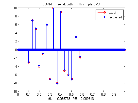
(a) ESPRIT: ฮผHโ€‹(S^,S)=0.057subscript๐œ‡H^๐‘†๐‘†0.057\mu_{\rm H}(\hat{S},S)=0.057RL.

Refer to caption

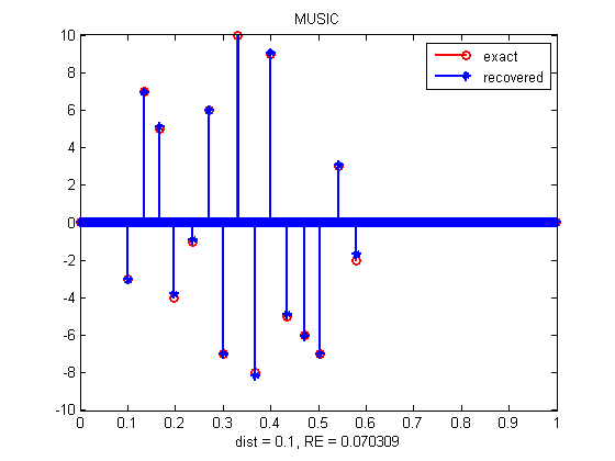
(b) MUSIC: ฮผHโ€‹(S^,S)=0.1subscript๐œ‡H^๐‘†๐‘†0.1\mu_{\rm H}(\hat{S},S)=0.1RL.

Figure 1: Reconstruction of 15 real-valued frequencies separated by 3-4 RL with 10%percent1010\% NSR.
Refer to caption
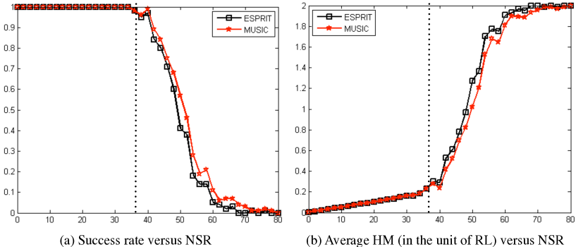
Figure 2: (a) Success rate and (b) average HM vs. NSR (in percentage) for separation of 2-3 RL

In conclusion, we have given performance guarantees for SS-ESPRIT. In particular, for noiseless measurement with M+1โ‰ฅ2โ€‹s๐‘€12๐‘ M+1\geq 2s, Theorems 1 and 2 guarantee exact recovery for any subset ๐’ฎโŠ‚[0,1]๐’ฎ01\mathcal{S}\subset[0,1] of s๐‘ s frequencies. For noisy measurement, Theorem 4 guarantees noise stability under the separation condition

ฯ>2โ€‹(1โˆ’4โ€‹ฯ€M)โˆ’12๐œŒ2superscript14๐œ‹๐‘€12\displaystyle\rho>2\Big{(}1-{4\pi\over M}\Big{)}^{-\frac{1}{2}}

in the unit of RL. This separation and sparsity constraint compares favorably with those of other approaches to compressed sensing in the continuum which are at least 3-4 RL [3, 4, 7, 8, 10, 21].

Numerical simulation demonstrates stability to a significant level of noise. The noise ฮต๐œ€\varepsilon is additive i.i.d. complex Gaussian, i.e. ฯตโˆผNโ€‹(0,ฮฝ2โ€‹I)+iโ€‹Nโ€‹(0,ฮฝ2โ€‹I)similar-toitalic-ฯต๐‘0superscript๐œˆ2๐ผ๐‘–๐‘0superscript๐œˆ2๐ผ\epsilon\sim N(0,\nu^{2}I)+iN(0,\nu^{2}I) of various strength in terms of the Noise-to-Signal Ratio (NSR)

NSR=๐”ผโ€‹{โ€–ฮตโ€–2}/โ€–yโ€–2=ฮฝโ€‹2โ€‹(M+1)/โ€–yโ€–2NSR๐”ผsubscriptnorm๐œ€2subscriptnorm๐‘ฆ2๐œˆ2๐‘€1subscriptnorm๐‘ฆ2\text{NSR}=\mathbb{E}\{||\varepsilon||_{2}\}/||y||_{2}=\nu\sqrt{2(M+1)}/||y||_{2}

where M=100๐‘€100M=100. The error metric the Hausdorff metric ฮผHโ€‹(๐’ฎ,๐’ฎ^)subscript๐œ‡H๐’ฎ^๐’ฎ\mu_{\rm H}(\mathcal{S},\widehat{\mathcal{S}}) between the exact ๐’ฎ๐’ฎ\mathcal{S} and recovered ๐’ฎ^^๐’ฎ\widehat{\mathcal{S}} sets of frequencies. We use two reconstruction methods: SS-ESPRIT analyzed above and MUSIC studied in [14] (see also [5, 6, 9, 13]) both of which employ the Hankel matrix (4) and the Vandermonde decomposition (5).

Fig. 1 shows an instance of reconstruction of 15 frequencies that are randomly distributed, separated by 3-4 RL and have real-valued amplitudes of dynamical range xmax/xmin=10subscript๐‘ฅmaxsubscript๐‘ฅmin10x_{\text{max}}/x_{\text{min}}=10, from M=100๐‘€100M=100 measured data of 10%percent1010\% NSR. Both ESPRIT and MUSIC perform well with comparable accuracy.

For Fig. 2, the frequency set ๐’ฎ๐’ฎ\mathcal{S} consists of 20 randomly selected frequencies separated by 2โˆ’3232-3 RL, with randomly phased amplitudes x๐‘ฅx of equal strength (i.e. the dynamic range xmax/xmin=1subscript๐‘ฅmaxsubscript๐‘ฅmin1x_{\text{max}}/x_{\text{min}}=1). A reconstruction is successful if ฮผHโ€‹(๐’ฎ^,๐’ฎ)โ‰ค1subscript๐œ‡H^๐’ฎ๐’ฎ1\mu_{\rm H}(\widehat{\mathcal{S}},\mathcal{S})\leq 1RL.

Fig.2(a) shows the success rate for 100 independent trials versus NSR. Clearly a โ€œphase transitionโ€ occurs at the threshold NSR โ‰ˆ37%absentpercent37\approx 37\% beyond which the success rate begins to drop precipitously. The threshold NSR depends on the frequency spacings, the numbers of data and frequencies as well as the dynamic range.

Fig.2(b) shows ฮผHโ€‹(๐’ฎ,๐’ฎ^)subscript๐œ‡H๐’ฎ^๐’ฎ\mu_{\rm H}(\mathcal{S},\widehat{\mathcal{S}}), averaged over 100 independent trials, versus NSR and exhibits the same phase transition where the rapid growth of ฮผHsubscript๐œ‡H\mu_{\rm H} is due to reconstruction failure. Notably the average ฮผHsubscript๐œ‡H\mu_{\rm H} below the threshold does not exceed 0.20.20.2RL, much better than the success criterion of 111RL.

Again the performances of ESPRIT and MUSIC are comparable in Fig. 2 with the main difference being the speed of computation: SS-ESPRIT is about ten times faster than MUSIC in our simulation.


Acknowledgements. Research is supported in part by US NSF grant DMS-1413373 and Simons Foundation grant 275037. I thank Lu Li for help in preparing the figures.

References

  • [1] R. Adamczak, โ€œA few remarks on the operator norm of random Toeplitz matricesโ€, J. Theoret. Probab. 23, pp.85-108, 2010.
  • [2] R. Badeau, G. Richard and B. David, โ€œPerformance of ESPRIT for estimating mixtures of complex exponentials modulated by polynomials,โ€ IEEE Trans. Signal Proc. 56(2), 492-504 (2008).
  • [3] E. J. Candรจs and C. Fernandez-Granda,โ€œSuper-resolution from noisy dataโ€, Journal of Fourier Analysis and Applications 19(6), pp.1229-1254, 2013.
  • [4] E. J. Candรจs and C. Fernandez-Granda, โ€œTowards a mathematical theory of super-resolutionโ€, Communications on Pure and Applied Mathematics 67(6), pp.906-956, June 2014.
  • [5] M. Cheney, โ€œThe linear sampling method and the MUSIC algorithmโ€, Inverse Problems 17(4), pp.591, 2001.
  • [6] M. Cheney, โ€œA mathematical tutorial on synthetic aperture radarโ€, SIAM review 43(2), pp.301-312, 2001.
  • [7] Y. Chi, A. Pezeshki, L. Scharf, A. Pezeshki, and R. Calderbank, โ€œSensitivity to basis mismatch in compressed sensingโ€, IEEE Transactions on Signal Processing 59(5), pp.2182-2195, 2011.
  • [8] L. Demanet, D. Needell and N. Nguyen, โ€œSuper-resolution via superset selection and pruningโ€, Proceedings of the 10th International Conference on Sampling Theory and Applications, 2013.
  • [9] A. Fannjiang, โ€œThe MUSIC algorithm for sparse objects: a compressed sensing analysisโ€, Inverse Problems 27, 035013, 2011.
  • [10] A. Fannjiang, and W. Liao, โ€œCoherence pattern-guided compressive sensing with unresolved gridsโ€, SIAM Journal on Imaging Sciences 5(1), pp.179-202, 2012.
  • [11] Y. Hua and T. K. Sarkar, โ€œMatrix pencil method for estimating parameters of exponentially damped/undamped sinusoids in noiseโ€, IEEE Transactions on Acoustics, Speech and Signal Processing 38(5), pp.814-824, 1990.
  • [12] A. E. Ingham, โ€œSome trigonometrical inequalities with applications to the theory of seriesโ€, Mathematische Zeitschrift 41(1), pp.367-379 (1936).
  • [13] A. Kirsch, โ€œThe MUSIC algorithm and the factorization method in inverse scattering theory for inhomogeneous mediaโ€, Inverse problems 18, pp. 1025-1040, 2002.
  • [14] W. Liao and A. Fannjiang, โ€œMUSIC for single-snapshot spectral estimation: stability and super-resolution,โ€ To appear in Appl. Comput. Harmon. Anal. arXiv:1404.1484.
  • [15] A. Paulraj, R. Roy, and T. Kailath, A subspace rotation approach to signal parameter estimation, Proceedings of the IEEE 74(7), 1044 - 1046 (1986).
  • [16] D. Potts and M. Tasche, โ€œ Parameter estimation for nonincreasing exponential sums by Prony-like methods,โ€ Linear Alg. Appl. 439, 1024-1039 (2013).
  • [17] R. Roy and T. Kailath, ESPRIT - Estimation of signal parameters via rotational invariance techniques, IEEE Trans. Acoustics, Speech, Signal Proc. ASSP-37(7), 984 - 995 (1989).
  • [18] R. O. Schmidt, โ€œMultiple emitter location and signal parameter estimationโ€, IEEE Trans. Antennas Propagat. 34(3), pp.276-280, 1986.
  • [19] G. W. Stewart and J. G. Sun, Matrix Perturbation Theory, 1990.
  • [20] P. Stoica and R. Moses, Spectral Analysis of Signals, Prentice Hall, New Jersey, 2005.
  • [21] G. Tang, B. Bhaskar, P. Shah, and B. Recht, โ€œCompressed sensing off the gridโ€, IEEE Transactions on Information Theory 59(11), pp. 7465-7490, 2013.
  • [22] R. M. Young, An Introduction to Nonharmonic Fourier Series, Academic Press, New York, 1980.