Plus Charge Prevalence in Cosmic Rays: Room for Dark Matter in the Positron Spectrum

Abstract

The unexpected energy spectrum of the positron/electron ratio is interpreted astrophysically, with a possible exception of the 100-300 GeV range. The data indicate that this ratio, after a decline between $0.5-8$ GeV, rises steadily with a trend towards saturation at 200-400GeV. These observations (except for the trend) appear to be in conflict with the diffusive shock acceleration (DSA) mechanism, operating in a single supernova remnant (SNR) shock. We argue that $e^{+}/e^{-}$ ratio can still be explained by the DSA if positrons are accelerated in a subset of SNR shocks which: (i) propagate in clumpy gas media, and (ii) are modified by accelerated CR protons. The protons penetrate into the dense gas clumps upstream to produce positrons and, charge the clumps positively. The induced electric field expels positrons into the upstream plasma where they are shock-accelerated. Since the shock is modified, these positrons develop a harder spectrum than that of the CR electrons accelerated in other SNRs. Mixing these populations explains the increase in the $e^{+}/e^{-}$ ratio at $E>8$ GeV. It decreases at $E<8$ GeV because of a subshock weakening which also results from the shock modification. Contrary to the expelled positrons, most of the antiprotons, electrons, and heavier nuclei, are left unaccelerated inside the clumps. Scenarios for the 100-300 GeV AMS-02 fraction exceeding the model prediction, including, but not limited to, possible dark matter contribution, are also discussed.

I Introduction

Recent measurements of a positron/electron, $e^{+}/\left(e^{-}+e^{+}\right)$, excess in the $8-300$ GeV range by Pamela, Fermi-LAT and AMS-02 (Pamela_Pos_09; Fermi_Pos_12; AMS_SepElPos14; AMS02_2014) has added fuel to the hotly contested race for elusive dark matter (DM) signatures in rapidly improving cosmic ray (CR) data (Hooper09; HooperDM_AMS13; Berezinsky2015JPhCS). Indeed, conventional acceleration schemes, even the most promising of them all, the diffusive shock acceleration (DSA), has not yet suggested any viable mechanism for the $e^{+}/\left(e^{-}+e^{+}\right)$ anomaly, free of tension with the antiproton spectra and other secondaries (Mertsch2009PhRvL; Kachelriess11; CholisHooper2014PhRvD).

In addition to the surprising excess at high energies, the $e^{+}/\left(e^{-}+e^{+}\right)$ ratio has a distinct minimum at $\approx 8$GeV which is not easier to explain making a minimum of assumptions. Both features appear at odds with the single source DSA operation, which predicts similar rigidity ($R=$momentum/charge) spectra for all primary species. Moreover, there are also other well documented exceptions, namely the He${}^{++}/p$ and $C/p$ ratios that both show a $\sim R^{0.1}$ growth, also seemingly inconsistent with the DSA (Adriani11; AMS02He2015PhRvL; AMS02andBessPtoHe2015). Less pronounced than $e^{+}/\left(e^{-}+e^{+}\right)$, but not less astonishing at first glance, these anomalies can be explained by the difference in charge to mass ratio (MDSPamela12). Other scenarios are possible but require additional assumptions, such as inhomogeneity of the SNR environment (Ohira11; Ohira15; Drury12) or multiple sources with adjusted spectral indices (see (Serpico15; Tomassetti2015ApJ; Ohira15) for a recent discussion). In fact, the mass to charge based explanation of the $\approx 0.1$ difference in rigidity indices has been given only for the He/$p$ spectrum, while the C/$p$ was measured with sufficient accuracy only recently (AMS02He2015PhRvL) and turned out to be identical to the He/$p$ rigidity spectrum. Thus, the mechanism suggested by (MDSPamela12) predicted the $C/p$ spectrum since He and C have the same mass to charge ratio. If this injection mechanism is correct, the latest AMS-02 data speak against a direct carbon acceleration from grains (Meyer97).

The mass to charge selectivity of the DSA which works for He/$p$ and C/$p$ does not apply to the $e^{+}/e^{-}$ fraction. It, therefore, seems logical to look for a possible charge-sign dependence of the SNR-DSA production of CRs, including the $e^{+}/\left(e^{-}+e^{+}\right)$ anomaly. We call it ’anomaly’ rather than ’excess’ (also encountered in the literature) since the ratio rises with the particle energy only at $E>8$GeV. Below this energy, it declines, thus creating a deficit. The decline, the rise and the clear minimum between them (at $8$ GeV) are all pivotal to the mechanism proposed here. These aspects are intrinsic to a single-source mechanism proposed, revealing unique characteristics of the accelerator. By contrast, assuming two or more independent positron contributions to the spectrum (as, e.g., in refs.(ErlykWolf2013APh; Mertsch2014PhRvD; Cowsik2014ApJ)), one fits the nonmonotonic positron fraction, but with no constraints on the underlying acceleration mechanisms. The position of the minimum in the positron fraction is then coincidental, and the fit does not add credibility to the model predictions for the higher energy data points yet to come. We will return to this point in the Discussion section.

A vast majority of conventional scenarios for the $e^{+}/\left(e^{-}+e^{+}\right)$ excess (including the present one) invoke secondary positrons. They are produced by galactic CR protons colliding with an ambient gas near an SNR accelerator, e.g. (Fujita2009PhRvD), elsewhere in the galaxy, e.g.,(Waxman2013PhRvL; Cowsik2014ApJ), or are immediately involved in the SNR shock acceleration, (Blasi2009PhRvL; Mertsch2014PhRvD; CholisHooper2014PhRvD). Some of these scenarios face the unmatched antiprotons and other secondaries in the data, as discussed, e.g., in (Kachelriess11; VladimirMoskPamela11; CholisHooper2014PhRvD). Improvements along these lines have recently been achieved by using Monte Carlo $pp$ collision event generators, e.g. (Kohri2016PTEP). However, improved cross sections of $pp$ collisions do not shed light on the physics of $e^{+}/\left(e^{-}+e^{+}\right)$ anomaly, particularly the minimum at 8 GeV. This spectrum complexity hints at richer physics than a mere production of secondary $e^{+}$ and $\bar{p}$ power-law spectra from the primary CR power-law.

We propose and investigate the idea that the physics of the $e^{+}/\left(e^{-}+e^{+}\right)$ fraction and, by implication, that of the $\bar{p}/p$ unmatched fraction, is in the charge-sign asymmetry of particle acceleration. The subsequent particle propagation through the galaxy or multiple accelerators plays no significant role in the phenomenon, as they act equally on all species. This proposition is particularly consistent with a scenario wherein almost all the positrons contributing to the observed $e^{+}/\left(e^{-}+e^{+}\right)$ ratio are produced in a single SNR of a particular kind described further in the paper. Electrons in the $e^{+}/\left(e^{-}+e^{+}\right)$ fraction may in part originate from an ensemble of other remnants. However, the single-source explanation for the $e^{+}/\left(e^{-}+e^{+}\right)$ anomaly is generic to all SNRs of the kind and thus is equally consistent with its multi-source origin. From the Occam’s razor perspective, this mechanism is preferred over those requiring different types of sources, to state the obvious.

A striking exception to the proposed scenario is the 100-300 GeV range where the current AMS-02 points significantly exceed our model predictions. This region then requires an independent source atop of the SNR contribution, that can be of a dark matter annihilation/decay or pulsar origin. Further model improvements are planned to see if simplifications made in its current version are responsible for the difference, but it appears to be unlikely.

The proposed mechanism relies on the following two aspects of the DSA. The first one is the injection process whereby particles become supra-thermal and may then cross and re-cross the shock front, thus gaining more energy. The proposed injection mechanism is charge-sign asymmetric. It differs from the conventional DSA in which the injection efficiency primarily depends on the mass-to-charge ratio but not so much on the sign of the charge (see, however, the Discussion section). We will argue that the charge-sign dependence of injection arises when the shock propagates into an interstellar medium (ISM) containing clumps of dense molecular gas (MC, for short).

The second aspect of the proposed mechanism concerns the phenomenon of nonlinear shock modification which is known to make the spectrum of low-energy particles steeper and that of the high-energy particles flatter than the canonical $p^{-4}$ spectrum produced by strong but unmodified shocks. Consequently, in the modified shocks, a point $p=p_{4}$ exists in the particle energy spectrum where the index is equal to four. Assuming that the bulk of galactic CR electrons are accelerated in conventional shocks, thus having $p^{-4}$ source spectra, the ratio of the modified positron spectrum to unmodified electron spectrum will show the required nonmonotonic behavior with a minimum at $p=p_{4}$. In a customary $p^{4}f$$\left(p\right)$ normalization, the individual positron spectrum is, therefore, the same as that of the $e^{+}/e^{-}$ ratio. Therefore, it conicides with the proton spectrum, provided all the species are relativistic. An analytic solution places the proton $p^{4}f$$\left(p\right)$ minimum at $\lesssim 10$ GeV/c (see Fig.5 in Ref. (MDru01)), depending weakly on the shock Mach number, $M$, proton maximum energy, $E_{{\rm max}}$, and their injection rate. However, $M\gtrsim 10$ and $E_{\max}\gtrsim 1$ TeV conditions are required, along with some minimum proton injection, for the solution to transition into a strongly nonlinear regime (often called efficient acceleration). Although the minimum in the spectrum looks encouraging for explaining the nonmonotonic $e^{+}/e^{-}$ ratio, it was obtained for protons and needs to be reconsidered for positrons in the 1-10 GeV/c momentum range. The reason for that is a different momentum dependence of positron and proton diffusivity (positrons enter a relativistic transport regime at much lower energy than protons).

Once an SNR shock is strongly modified, MCs in its precursor will survive the sub-shock UV and X- radiation, severely diminished in such shocks. At the same time, shock-accelerated CR protons illuminate the MC well before the subshock encounter. These CRs generate positrons (along with other secondaries) in the MC interior by colliding with the dense gas material. The CR protons also charge the MC positively; as a result, many positively charged particles abandon the MC, while negatively charged particles remain inside. Being charged by the shock-accelerated protons, the MC thus acquires a positive potential which creates a charge-sign asymmetry for the subsequent particle injection into the DSA.

Plasmas are intolerant to external charges and immediately restore charge neutrality. Nevertheless, a large and dense MC needs to build up a strong electric field to restore charge neutrality. Due to the high rigidity of CRs, their density in the MC interior increases almost simultaneously with that in the exterior, as a CR-loaded shock approaches the MC. However, by contrast with a strongly ionized exterior, where the plasma resistivity is negligible, the electron-ion, ion-neutral (and, in the case of very dense clouds, also electron-neutral) collisions inside the MC, provide significanty resistivity to the neutralizing electric current. Therefore, a strong macroscopic electric field is generated in response to the CR penetration. This field expels the secondary positrons most efficiently as the lightest positively charged species – although it also shields the MC from low-energy CR protons.

The mechanism outlined above implies that negatively charged primaries and secondaries have much better chances to stay in an MC than positively charged particles. When the subshock eventually reaches the MC, the subshock engulfs it, e.g., (Inoue12; Draine2010BookISM). What was inside of the MC, is transferred downstream unprocessed by the subshock. Therefore, the negatively charged particles in its interior largely evade acceleration. This charge-sign asymmetry of particle injection into the DSA explains why there is no $\bar{p}/p$ excess, similar to that of $e^{+}/e^{-}$ .

It follows that the positron spectrum results from several interwoven processes. We will consider them separately and study their linkage. The remainder of the paper is organized as follows. Sec.II deals with a spatial distribution of CR in a shock precursor, their propagation inside of an MC and electrodynamic processes that the CR induce there. In Sec.III we discuss and estimate the distribution of secondary positrons as they come out of the MC and become subject to the DSA. The spectrum of accelerated positrons is calculated from low to high energies, and the nature of the 8 GeV minimum is elucidated. We briefly discuss some of the alternative explanations of the $e^{+}/\left(e^{-}+e^{+}\right)$ excess in Sec.IV, followed by the Conclusion section, Sec.V.

II Interaction of shock-accelerated
protons with MC

An MC illumination by shock-accelerated CR protons before the shock arrival is crucial for the mechanism of positron injection into the DSA. The protons begin interacting with the MC when its distance to the subshock shortens to the CR diffusion length $\sim\kappa/u_{1}$, Fig.1. Here $\kappa$ is the CR diffusion coefficient and $u_{1}$ is the shock velocity. Generally, $\kappa$ depends on the CR momentum, e.g., in a Bohm limit, $\kappa\simeq cr_{g}\left(p\right)/3$, where $r_{g}$ is the CR gyro-radius. As $\kappa$ grows with $p$, higher energy protons reach the MC earlier. To understand the electrodynamic response of the MC to the penetrating CRs, we need to know their number density depending on the subshock distance. This subject is addressed in the next subsection.

II.1 CR spatial profile in unshocked plasma

The simplest assumption to start with is that CRs penetrate freely into an MC with an implication that their number density, $n_{CR}$, inside the MC depends only on the distance to the subshock, $x_{MC}$. The assumption is reasonable for high energy CRs and small MCs, as the CRs penetrate the MC more easily and omnidirectionally in this case. It is generally not valid for large MCs (MDS_APS12), which we discuss in Appendix A. We also show there that, in a wide range of conditions, the CR number density can be approximated by

$$n_{CR}\left(x\right)=\frac{x_{0}n_{CR}^{0}}{x_{0}+x_{MC}}$$ (1)

Here $n_{CR}^{0}$ is the CR density at the subshock ($x_{MC}=0$) and $x_{0}$ weakly depends on the CR momentum distribution. Note that the last expression is virtually independent of the degree of shock modification. However, in modified shocks the flow velocity gradually decreases from its far upstream value $u_{1}$ to $u_{0}$ ahead of the subshock, where it drops abruptly to $u_{2}<u_{0}$ downstream, Fig.2. The total shock compression ratio $r=u_{1}/u_{2}$ depends on the shock Mach number and the CR pressure (MDru01) and may be much higher than the typical value of four. The subshock compression ratio, $r_{s}=u_{0}/u_{2}$ can, in turn, be significantly lower than four.

While the plasma slows down towards the subshock, an MC proceeds at a higher speed, Fig.2 because the CR pressure and the ram pressure of the plasma are insufficient to slow down dense clouds considerably. Thus, the MCs encounters a supersonic headwind (for $u_{1}-u_{0}>C_{s}$, the sound speed) and a bow-shock must form on the shock side of the MC. However, we will not discuss this further in the paper. Instead, we focus on the plasma processes in the MC interior initiated by penetrating CR protons. In what follows, we assume them to have enough energy to cross the possible bow-shock and the MC-plasma interface unimpededly.

As a rule, plasmas respond promptly to external charges and readily restore its neutrality due to high electric conductivity. But when energetic protons penetrate into a more resistive plasma inside an MC, a stronger electric field needs to build up to neutralize the charge, and there are several neutralization scenarios to consider. First, because of the electric field, the MC plasma may suck in external thermal electrons. Again, the MC plasma is electrically resistive due to a high neutral density and low temperature. Therefore, the efficiency of this neutralization is limited, and the electrostatic potential inside the MC may grow considerably to sustain the charge neutrality, possibly up to an electric breakdown of the MC neutral gas with significant pair production (GurevichPairs00). Another limitation comes from the total flux of thermal electrons entering the MC. It cannot significantly exceed the value $\sim V_{Te}n_{0}S$, where $n_{0}$ and $V_{Te}$ are the electron density and thermal velocity, while $S$ is the effective MC cross section across the magnetic field. (We neglect the cross-field particle transport here and below, including that of the CRs).

To facilitate our discussion of the MC neutralization, we introduce a charge budget parameter, $\eta$, as a ratio of the MC charging rate by CR protons to its neutralization rate by inflowing extraneous electrons and outflowing MC ions:

$$\eta=\frac{\dot{n}_{{\rm CR}}L_{{\rm MC}}}{V_{Te}n_{0}+V_{i}n_{i}}\sim\frac{L_{{\rm MC}}}{L_{{\rm CR}}}\cdot\frac{u_{1}n_{{\rm CR}}}{V_{Te}n_{0}+V_{i}n_{i}}$$ (2)

Here $\dot{n}_{CR}=dn_{CR}/dt$ is the CR charging rate, $n_{i}$ and $V_{i}$ are the density and velocity of the ions at the MC boundaries, $x=\pm a$. We count the $x$- coordinate from the center of the MC along the field line, Fig.1. The characteristic time of CR increase in the MC (also the CR maximum acceleration time) is $t_{a}\sim L_{CR}/u_{1}$, where $L_{CR}\sim\kappa\left(p_{{\rm max}}\right)/u_{1}$ is the CR precursor scale-height and $u_{1}$ is the shock velocity. At least initially, the charge neutralizing current is carried by the thermal electrons (first term in the denominator). However, it does not increase in response to the growing electric field as this flux is fixed by the ambient plasma conditions, not affected by the MC. By contrast, the ion contribution to the CR neutralization (second term in the denominator in eq.[2]) is dynamic and becomes more important when the electric field accelerates the outflowing ions. At the same time, the resulting ion depletion inside the MC may eventually diminish neutralization. It follows that the parameter $\eta$, although small in general, may grow significantly, especially in strong SNR shocks where $u_{1}\gg V_{Te}$. The resulting electric field $E\left(x\right)$ clearly depends on $\eta$ so that we include the above aspects in an equations for $E$ in the next subsection.

The time dependence of $n_{CR}\left(t\right)$ regulates an MC charging. We substitute $n_{CR}\left(x\right)$ from eq.(1) and assume that the MC propagates ballistically through the shock precursor, that is we can write $x_{MC}=-u_{1}t$, where $-\infty<t\leq 0$ and the subshock reaches the MC at $t=0$. Therefore, $n_{CR}$ grows in time as

$$n_{CR}\left(t\right)=n_{CR}^{0}x_{0}/\left(x_{0}-u_{1}t\right)$$ (3)

As $n_{CR}$ grows rapidly when the MC approaches the subshock (the growth stops when $n_{CR}$ reaches $n_{CR}\left(t=0\right)=n_{CR}^{0}$), the following reaction from the MC is expected. First, the increase in $\eta$ may slow down, as the electric field ejects more ions from the MC. But, when many of them are expelled and the ion flux $V_{i}n_{i}$ cannot balance the continuing $n_{CR}$ increase, the electric field inside the MC may exceed the ionization threshold. As a result, the $n_{i}$ will increase, thus limiting $\eta$, or even an electric breakdown of the gas becomes possible, as mentioned earlier. We defer this issue to future work and consider in the next subsection the build-up of an electrostatic potential inside the MC, as the latter is charged by penetrating CRs with neglected ionization and recombination.

II.2 Electrodynamics of CR-MC interaction

For describing an MC response to penetrating CR protons, we use two-fluid equations for electrons and ions that move along the $x-$axis (magnetic field direction, Fig.1) in the MC interior:

$$\frac{dV_{i}}{dt} = \frac{e}{m_{i}}E\left(x,t\right)-\nu_{in}V_{i}$$

$$\frac{dV_{e}}{dt} = -\frac{e}{m_{e}}E-\nu_{ei}\left(V_{e}-V_{i}\right)$$

$$\frac{\partial n_{e,i}}{\partial t} = -\frac{\partial}{\partial x}n_{e,i}V_{e,i}$$

$$n_{e} = n_{i}+n_{CR}$$

where

$$\frac{d}{dt}\equiv\frac{\partial}{\partial t}+V_{i}\frac{\partial}{\partial x}$$

Here $V_{i,e}$ and $n_{i,e}$ are the mass velocities and number densities of electron and ion fluids, $E=-\partial\phi/\partial x$ is the electric field, $\nu_{in}$ and $\nu_{ei}$ are the ion-neutral and electron-ion collision frequencies. The last equation is the usual quasi-neutrality condition replacing the Poisson equation because $L_{MC}$ exceeds the Debye radius by many orders of magnitude. On comparing the first two equations, we neglect the electron inertia term in the second equation, after which it suggests eliminating the electron velocity $V_{e}$ altogether. Furthermore, by taking the difference between the continuity equations for electrons and ions, and introducing the CR column density inside the MC, $N_{CR}$, by the relation $n_{CR}=\partial N_{CR}/\partial x$, the above system of five equations may be manipulated into the following two equations:

$$\frac{dV_{i}}{dt} = -\nu_{in}V_{i}+\frac{m_{e}}{m_{i}}\left(\dot{N}_{CR}+n_{CR}V_{i}\right)\frac{\nu_{ei}}{n_{CR}+n_{i}}$$ (4)

$$\frac{dn_{i}}{dt} = -n_{i}\frac{\partial V_{i}}{\partial x}$$ (5)

The dot over $N_{CR}$ stands for a time derivative. The second term on the r.h.s. of eq.(4) is proportional to the electric field,

$$E\left(x,t\right)=\frac{m_{e}}{e}\nu_{ei}^{\prime}\frac{n_{CR}n_{i}}{n_{CR}+n_{i}}\left(\frac{\dot{n}_{CR}}{n_{CR}}x+V_{i}\right),$$ (6)

where we have ignored variations of CR density inside the MC and used the linear approximation for $N_{CR}\approx n_{CR}x$, along with a symmetry requirement, $E=V_{i}=0$ at $x=0$ (center of MC). We have also separated the ion density from collision frequency $\nu_{ei}$, by introducing the following parameter

$$\nu_{ei}^{\prime}=\frac{4}{3}\sqrt{2\pi}\frac{e^{4}}{\sqrt{m}T_{e}^{3/2}}\Lambda=\nu_{ei}/n_{i}$$

where $\Lambda\sim 10$ is a Coulomb logarithm. The ion-neutral collision frequency can be written as follows

$$\nu_{in}=\frac{8\sqrt{2}}{3\sqrt{\pi}}\sigma_{in}n_{n}\sqrt{\frac{m_{i}T}{m_{n}\left(m_{n}+m_{i}\right)}}$$

with the ion-neutral collision cross section $\sigma_{in}\approx 5\cdot 10^{-14}cm^{2}.$ We neglect the electron-neutral collisions, since $\sigma_{en}\approx 4\cdot 10^{-15}$. These and other parameters, pertinent to MCs, are summarized, e.g., in (Dogiel1987MNRAS). Using the above approximation of coordinate independent $n_{CR}$ ($N_{CR}\approx n_{CR}x$), we will convert the system given by eqs.(4-5) into a system of two ordinary differential equations but first, we introduce some dimensionless variables. It might appear natural to measure time in precursor crossing times, $t_{a}=L_{CR}/u_{1}=\kappa\left(p_{{\rm max}}\right)/u_{1}^{2}$, Fig.2. However, since our focus here is on processes occurring inside the MC, as it traverses the shock precursor, the MC travel time $t_{a}$ is not the best time unit. Indeed, the main driver of these processes is the changing $n_{CR}\left(t\right)$ which is nearly scale free, eq.(3). It is, therefore, more convenient to choose $\nu_{in}^{-1}$ for the time unit. Denoting by $2a$ the length of a given field line, to which eqs.(4-5) refer inside the MC (Fig.1), we use the following scales of the remaining variables:

$$\frac{x}{a}\to x,\;\;\nu_{in}t\to t,\;\;\;\frac{V_{i}}{\nu_{in}a}\to V_{i},\;\;\;\frac{n_{i}}{n_{0}}\to n_{i},\;\;\;\frac{n_{CR}}{n_{0}}\to n_{CR}$$

where $n_{0}$ is the initial ion density. Eqs.(4-5) rewrite then as follows:

$$\frac{\partial V_{i}}{\partial t} = -V_{i}\frac{\partial V_{i}}{\partial x}-V_{i}+\nu_{e}\frac{n_{CR}n_{i}}{n_{CR}+n_{i}}\left(\frac{\dot{n}_{CR}}{n_{CR}}x+V_{i}\right)$$ (7)

$$\frac{\partial n_{i}}{\partial t} = -n_{i}\frac{\partial V_{i}}{\partial x}-V_{i}\frac{\partial n_{i}}{\partial x}$$ (8)

where we introduced the following collision parameter

$$\nu_{e}=\frac{m_{e}}{m_{i}}\frac{\nu_{ei}^{\prime}n_{0}}{\nu_{in}}.$$

We need to solve eqs.(7) and (8) in the domain $-1<x<1$. For $a\ll L_{CR}$, or roughly also for $a\lesssim L_{CR}$ and a quasiperpendicular shock geometry, the following symmetry conditions are suggestive, $\mbox{$n_{i}\left(-x\right)=n_{i}\left(x\right),$ }V\left(-x\right)=-V\left(x\right)$ (see also Appendix A). They require the following boundary conditions at $x=0$: $\partial n_{i}/\partial x=0,\;\;V=0$. Note that the shock geometry becomes progressively quasiperpendicular towards the subshock by virtue of compressed magnetic field component in the shock plane, Fig.1. The electric field $E$ will have the same symmetry properties as $V.$ With the above boundary conditions, eqs.(7- 8) admit the following simple form of solution

$$n_{i} = n_{i}\left(t\right)$$ (9)

$$V = \psi\left(t\right)x$$ (10)

so that eqs.(7-8) reduce to an ODE system:

$$\frac{d\psi}{dt} = -\psi^{2}-\nu_{i}\psi+\frac{\nu_{e}n_{i}}{n_{CR}+n_{i}}\left(\dot{n}_{CR}+n_{CR}\psi\right)$$ (11)

$$\frac{dn_{i}}{dt} = -\psi n_{i}$$ (12)

An assumption $n_{CR}\ll n_{i}$ greatly simplifies the first equation of this system and allows us to solve it independently of the second one. The assumption remains plausible during an initial phase of the MC-CR interaction, but it may be violated at later times when $n_{CR}$ increases while $n_{i}$ decreases because of the ion outflow. When the condition holds up, the solution of the second equation can be readily obtained in terms of $\psi,$ while the first equation makes a Riccati equation for $\psi$. After this equation is solved we will constrain the problem parameters to ensure the condition $n_{CR}\ll n_{i}$.

The solution to eq. (11) is obtained in Appendix B , and the transition from the PDE to ODE is justified by a direct numerical integration of the original PDE system, given by eqs.(7-8). We can write the solution for $\psi$ as follows

$$\psi\left(\tau,\alpha\right)=\frac{\alpha}{\tau}-1+\frac{\tau{}^{\alpha}e^{-\tau}}{\Gamma\left(\alpha+1,\tau\right)}$$ (13)

where $\Gamma$ is an incomplete gamma-function,

$$\Gamma\left(\alpha+1,\tau\right)\equiv\int_{\tau}^{\infty}t^{\alpha}e^{-t}dt$$

and $\tau=t_{0}-t$. The dimensionless parameters $\alpha$ and $t_{0}$ are defined in eq.(52), $t_{0}=\nu_{in}a/u_{1}$, $\alpha=\left(m_{e}/m_{i}\right)\left(\nu_{ei}a/u_{1}\right)\left(n_{CR}^{0}/n_{i}\right)$. The density depletion of the MC ions can now be obtained from eq.(12):

$$\frac{n_{i}\left(t=0\right)}{n_{i}\left(t=-\infty\right)}=\left[\int_{t_{0}}^{\infty}\left(\tau/t_{0}\right)^{\alpha}e^{t_{0}-\tau}d\tau\right]^{-1}$$ (14)

where $t=-\infty,0$ refer to the far upstream ion density, $n_{i}$, and its value when the subshock intersects the MC. Whether the above ratio can be considerably smaller than unity, thus possibly violating the assumption $n_{CR}\ll n_{i}$, depends on the parameter $\alpha/t_{0}$. This is because a saddle point on the phase integral in eq.(14) is on the integration path for $\alpha>t_{0}$, thus making a large contribution to the integral. So, one can estimate the integral as follows

$$\int_{t_{0}}^{\infty}\left(\tau/t_{0}\right)^{\alpha}e^{t_{0}-\tau}d\tau=\begin{cases}1+\alpha/t_{0},&\alpha/t_{0}<1\\ \sqrt{2\pi\alpha}\left(\alpha/t_{0}\right)^{\alpha}e^{t_{0}-\alpha},&\alpha/t_{0}>1\end{cases}$$

To reconstruct possible scenarios of MC neutralization, we take a closer look at the parameter $\alpha/t_{0}$ in eq.(52). Assuming for simplicity that $T_{e}\sim T_{i}$ inside the clump, the following estimate can be obtained:

$$\frac{\alpha}{t_{0}}\sim\left(\frac{1eV}{T_{e}}\right)^{2}\frac{n_{CR}^{0}}{n_{n}}\sqrt{\frac{m_{n}}{m_{i}}\left(\frac{m_{n}}{m_{i}}+1\right)\frac{m_{e}}{m_{i}}}$$

Unless the neutral density $n_{n}$ and electron temperature $T_{e}$ in the MC interior are fairly low, the above parameter is not larger than one, so the density depletion, $\Delta n_{i}/n_{i}\simeq\alpha/t_{0}\ll 1$, remains insignificant during the MC travel through the shock precursor. This estimate validates our assumption $n_{CR}\ll n_{i}$ and thus the solution given by eq.(13).

The weak effect of accelerated CR protons on the MC ion density does not mean that the charge neutralizing electric field also remains weak. The electric field can be determined from eqs.(6,10,13), so we can write it as follows

$$E\left(x,t\right)\simeq\frac{m_{i}}{e}a\nu_{in}^{2}\frac{x\alpha}{\left(t_{0}-t\right)^{2}}\left[1+\frac{\alpha}{t_{0}-t}\right]$$

where $E$ is given in physical units, while $x$, $t_{0}$ and $t$ are still dimensionless, stemming from the expansion of $\psi(\alpha,t)$ for small $\alpha/t_{0}$. The second term in the brackets corresponds to the ion contribution to electric field generation (second term in the brackets in eq.[6]). As long as $\Delta n_{i}/n_{i}\simeq\alpha/t_{0}\ll 1$, it can be neglected. The electric field reaches its maximum at the edge of MC at the moment of subshock encounter, $t=0$. It can be represented as

$$E_{{\rm max}}\simeq\frac{m_{e}}{e}u_{1}\nu_{ei}\frac{n_{CR}^{0}}{n_{i}}$$ (15)

There are two potentially significant effects of the electric field. First, it may cause a runaway acceleration of thermal electrons. To assess this possibility, one needs to compare $E_{{\rm max}}$ with a critical (Dreicer) field, above which many electrons from the thermal Maxwellian gain more energy from the field between collisions than they loose after the collisions (pitaevskii1981physical). From the last formula we obtain

$$\frac{E_{{\rm max}}}{E_{{\rm crit}}}\sim\frac{u_{1}}{V_{Te}}\frac{n_{CR}^{0}}{n_{e}}$$ (16)

We observe that the collision frequency quite naturally cancels out in this ratio. It thus depends only on the ratio of the convective CR flux to that of the thermal electrons. It should also be noted that to produce a significant effect, $E_{{\rm max}}$ does not need to be close to $E_{{\rm crit}}$. Even if the above ratio is low, an exponentially small number of runaway electrons (Gurevich61RunAway) on the tail of their velocity distribution can initiate an ionization process. Once started, it may develop into a gas breakdown at fields significantly below the impact ionization threshold (GurevichPairs00). The runaway breakdown, actively studied in terrestrial thunderstorms, requires a seed population of fast electrons, sporadically produced by ionizing CRs (GurevichUFN2001). In an MC ahead of an SNR shock such population is readily available, e.g., from shock accelerated electrons and secondary electrons inside the MC. Another possible effect associated with the runaway process is an electromagnetic cascade that may result in a pair production which would further increase the number of positrons injected into the DSA. These phenomena, expected to occur in strong electric fields, will react back on the field generation by increasing the neutralizing current. The runaway electrons, in particular, may carry most of that current.

The electrostatic potential that obviously has a maximum in the middle of the MC may partially screen the MC interior from the penetrating CR, particularly a low-energy and, therefore, more intense part of their spectrum. The maximum potential is proportional to the MC half-length, $a.$ To determine the CR penetration into the MC, one needs to compare this potential with the proton rest energy, $m_{p}c^{2}$. So, from eq.(6) we obtain

$$\frac{e\phi_{{\rm max}}}{m_{p}c^{2}}\sim\frac{a}{1pc}\frac{u_{1}}{c}\frac{n_{CR}}{1cm^{-3}}\left(\frac{1eV}{T_{e}}\right)^{3/2}$$ (17)

Similarly to the comparison of the electric field with the critical Dreicer field in eq.(16), the last estimate also places the field potential in a critical range, this time, possibly close to the relativistic proton energy. A one-parsec size MC does not appear implausible, as it would be of the order of the gyroradius of a PeV (knee energy) proton. Such an MC occupies only a $u_{1}/c\ll 1$- fraction of the entire CR precursor, assuming Bohm diffusion regime. The above estimates indicate that the electric field may grow strong enough to react back on the penetration of low-energy CRs into the MC and neutralization of the CR charge by a plasma return current. These aspects of the CR-MC interaction require a separate study. Here, we assume the relevant parameters constrained as to keep the ratios in eqs.(16) and (17) significantly smaller than one.

III Spectrum of shock-accelerated positrons

In Sec.II.2 we have considered relevant MC processes driven by penetrating CRs. We have found the CR density, MC electrostatic potential, and ion outflow velocity increasing explosively, $\propto\left(t_{0}-t\right)^{-1}$, towards the subshock encounter. Therefore, the positron expulsion from the MC will culminate at the time of encounter, thus peaking their injection into the DSA process discussed further in this section.

III.1 Positron Injection into DSA

Being interested in a particle injection from many MCs, occasionally crossing the shock, we may consider the expelled positrons as injected into the DSA at time-averaged rate $Q\left(p,x_{MC}\right)$. It decays sharply with $x_{MC}$, the distance from the subshock, according to eq.(1) which is more convenient to use here than its time-dependent analog, given in eq.(3). In what follows, we will write $x$, instead of $x_{MC}$ which should not cause any confusion with the notation of Sec.II.

A momentum distribution of injected positrons is determined by the history of their production in, and outflow from, an MC. At large distances from the subshock, only the most energetic CRs penetrate the MC, while low-energy CRs do not reach it. On the other hand, short before shock crossing, the low-energy CRs cannot freely penetrate the MC, because of the induced electric field. Thus, bearing in mind that positrons receive only a few percent of the energy of parent protons, it is not unreasonable to expect $Q\left(p\right)$ having a relatively broad maximum near or somewhat below the momentum $e\phi_{{\rm max}}$/c, eq.(17). Given relatively cold, e.g., $T_{e}\sim 100$K electrons in the MC, this maximum is likely to be in a sub-GeV range. Here we orient ourselves towards a cold neutral medium with $n_{{\rm H}}\gtrsim 30{\rm cm^{-3}}$ and the filling factor $f_{V}\sim 0.01$ (Chev03; Draine2010BookISM). The value of $n_{{\rm H}}f_{V}$ may substantially exceed its counterpart in the ambient plasma.

Positrons, generated in CR-MC gas collisions are confined in the MC for a time $\tau_{{\rm conf}}\sim a^{2}/\kappa\left(p\right),$ to be compared with the precursor crossing time (also CR acceleration time) $\tau_{a}\sim\kappa\left(p_{{\rm{\rm max}}}\right)/u_{1}^{2}\sim L_{CR}/u_{1}$. Here $p$ and $p_{{\rm max}}$ denote the positron and maximum CR (proton) momentum, respectively. Strictly speaking, the particle diffusivities $\kappa$ are different, as they refer to different media (MC and ionized CR precursor). Nonetheless, for a simple estimate below, we may adopt the Bohm scaling for both. If $\tau_{{\rm conf}}/\tau_{a}\gg 1$, which translates then into $p/p_{{\rm max}}\ll a^{2}/L_{CR}^{2}$, low-energy secondary positrons accumulated in the MC over the precursor crossing time, will stay inside the MC. Therefore, they will avoid the DSA process, along with the most of negatively charged particles. Indeed, a strongly weakened subshock engulfs the MC without shocking its material over the MC crossing time (Draine2010BookISM; Inoue12). To a certain extent, this also relates to the positively charged secondaries and spallation products, diffusively trapped in the MC. Therefore, they do not develop spectra similar to that of the positrons.

Two considerations help to elaborate the above constraint on the positron momentum $p$. First, a significant modification of the shock structure requires a proton cut-off momentum $p_{{\rm max}}\gtrsim 1$ TeV, while our interest in positrons is limited to $p<500$ GeV (data availability). Second, the positrons receive, on average, only about 3 percent of the energy of parent CRs. These considerations render $p/p_{{\rm max}}\ll 1$ as a strong inequality. We, therefore, conclude that except for very small MCs, the condition $p/p_{{\rm max}}\ll a^{2}/L_{CR}^{2}$ is fulfilled and most of the early generation of positrons, produced by high-energy protons, will stay inside the MC. However, in parameter regimes when the electric field is very strong, this conclusion may be violated but we assume that it is not.

On entering the subshock proximity, the CR number density sharply increases by GeV particles. To some extent, these particles are screened by an MC electric field which reaches its maximum at the MC’s edge. Therefore, they generate secondary $e^{\pm}$ and, for that matter, $\bar{p}$, at the periphery of the MC. The edge electric field then expels positively charged secondaries ($e^{+}$) and sucks in negatively charged ones, such as $e^{-}$ and, to some extent, $\bar{p}$, even though they are considerably more energetic for kinematic reasons. Based on the calculation of the field in Sec.II.2, the typical energy of expelled positrons should not exceed $1-2$ GeV. This estimate is consistent with that presented earlier in this subsection.

Now we turn to the acceleration of injected positrons. It should be noted, however, that some secondary negatively charged particles, such as $\bar{p},$ can still be injected along, particularly if the MC is sufficiently small and the maximum field potential is thus not high enough to suck them in. In this paper, however, we do not consider their contribution to the integrated CR spectrum produced in an SNR of the type considered. Such consideration would require us to address the question of the MC distribution in size.

III.1.1 Shock Acceleration of Positrons

Upon expulsion from an MC, positrons undergo the DSA. As the shock is strongly modified, the acceleration starts in its precursor. Because of the flow convergence, $\partial u/\partial x\neq 0$, particles gain energy without even crossing the subshock (MD06). On the other hand, most of the positrons are released from the MC near the subshock. Thus, at lower energies, their spectrum will be dominated by the subshock compression ratio, $r_{s}=u_{0}/u_{2}$ rather than by the precursor precompression, $u_{1}/u_{0}$. Therefore, the spectral index must be $q=q_{s}\equiv 3r_{s}/\left(r_{s}-1\right)$ and the spectrum $f_{e^{+}}\propto p^{-q_{s}}$.

By gaining energy, particles sample progressively larger portions of shock precursor with higher compression ratios, Fig.2, which makes their spectrum harder. On the other hand, as they also need to diffuse across larger portions of the precursor, the acceleration slows down which makes the spectrum softer. Asymptotically, these trends balance each other, but the balance is critically supported by accelerated protons, and their pressure needs to be included in the equations for the shock structure. In the case of very strong shocks ($M\to\infty$) with sufficiently high maximum energy, a universal spectrum $p^{-3-\sigma/2},$ establishes (MDru01). Here $\sigma$ is the index of particle diffusivity, $\kappa\propto p^{\sigma}$ with $\sigma=1$ for Bohm diffusion.

Consider now the ratio of positron spectrum to the spectrum of electrons produced in unmodified strong shocks with a typical spectrum $\propto p^{-4}$. This ratio, that is $p^{4}f_{e^{+}}\left(p\right)$, will have a decreasing branch at low momenta, since $f_{e^{+}}\left(p\right)\propto p^{-q_{s}}$ with $q_{s}>4$, and an increasing branch at high momenta, where the positron spectral index tends to 3.5. The remainder of this section deals with the calculation of positron spectrum described above, by solving the diffusion-convection equation, and comparisons with the AMS-02 data.

It is convenient to place the upstream medium in the $x>0$ half-space, with the subshock at $x=0$, but use positive quantities in describing the flow velocity. In the subshock frame, the physical flow velocity starts from $-u_{1}$ at $x=\infty$, decreases gradually to its value $-u_{0}$ just ahead of the subshock, and then jumps to its downstream value $-u_{2}$: $0<u_{2}<u_{0}\leq u\left(x\right)<u_{1}$, Fig.2. We will ignore the inclination of the magnetic field line to the shock normal (i.e. $x-$ direction), which can be effectively included by redefining the diffusion coefficient (Drury83).

Although the dynamics of an individual MC is essentially time dependent (Sec.II.2), we are interested in an average positron input from an ensemble of MCs. Therefore, we consider a steady state problem with a stationary injection of positrons at the subshock. The injection rate is then given by a time averaged source $Q\left(x,p\right)$, discussed in Sec.III.1. The distribution of accelerated positrons is governed by the familiar convection-diffusion equation

$$u\frac{\partial f}{\partial x}+\kappa\left(p\right)\frac{\partial^{2}f}{\partial x^{2}}=\frac{1}{3}\frac{\partial u}{\partial x}p\frac{\partial f}{\partial p}-Q\left(p,x\right),$$ (18)

with a standard normalization of the positron number density:

$$n_{e^{+}}\left(x\right)=\int f\left(x,p\right)p^{2}dp,$$

The momentum dependence of the positron diffusion coefficient $\kappa$ can be taken to be in an ultrarelativistic Bohm regime, $\kappa=\kappa^{\prime}p,$ with $\kappa^{\prime}=const.$

First, we consider the solution to eq.(18) for moderate values of $p$, assuming that the positron diffusion length, $\kappa\left(p\right)/u_{0}\ll L_{CR}$, where, $L_{CR}\sim\kappa\left(p_{{\rm max}}\right)/u_{1}$ is the precursor scale, determined by the maximum energy of accelerated protons. Hence, we may expand the flow velocity upstream, $u\left(x\right)=u_{0}+u^{\prime}x$, for $x\geq 0$ with $u^{\prime}=const$. At the same time, we will focus on particle momenta that are higher than the injection momentum, so we drop the injection term $Q$ in eq.(18) and include its effect on the solution in form of normalization of $f$. In particular, the value $f\left(x=0,p=p_{{\rm inj}}\right)$, where $p_{{\rm inj}}$ is defined as $Q\left(p>p_{{\rm inj}}\right)=0,$ can be expressed through injection rate $Q$ approximately as

$$f\left(0,p_{{\rm inj}}\right)\approx\frac{1}{u_{0}}\int_{0}^{\infty}Qdx,$$ (19)

We have assumed here that, in a steady state considered, injection is balanced by convection at low momenta. For that reason, we have neglected diffusion and acceleration terms, according to $\kappa/u_{0}l_{inj}\ll 1$ and $u_{1}l_{inj}/L_{CR}u_{0}\ll 1$. More accurate determination of the normalization is not worth the effort, as there are larger uncertainties in the value of $Q$, associated with our limited knowledge of the MC density, for example. The main objective here is to determine the spectral shape of $e^{+}$ which does not depend on the normalization, as the shock modification is produced by protons, not positrons.

To lighten notation, we make use of invariant properties of Eq.(18), and replace $\kappa\left(p\right)=\kappa^{\prime}p\to p$, which can easily be reversed by the transform $p\to\kappa$, when the equation is solved . Note that a more general scaling of $\kappa$ with $p$, such as $\kappa\propto p^{\sigma}$ can also be accommodated by a simple change of variables/coefficients. Adhering to the Bohm scaling, and taking all the above considerations into account we rewrite eq.(18) as

$$\left(u_{0}+u^{\prime}x\right)\frac{\partial f}{\partial x}+p\frac{\partial^{2}f}{\partial x^{2}}=\frac{1}{3}u^{\prime}p\frac{\partial f}{\partial p}$$ (20)

This equation can be readily solved by applying a Laplace transform

$$f_{\lambda}\left(p\right)=\int_{0}^{\infty}f\left(p,x\right)e^{-\lambda x}dx,$$

which yields

$$u^{\prime}\left(\lambda\frac{\partial f_{\lambda}}{\partial\lambda}+\frac{p}{3}\frac{\partial f_{\lambda}}{\partial p}\right)-\left(u_{0}\lambda+\lambda^{2}p-u^{\prime}\right)f_{\lambda}=-\left(u_{0}+\lambda p\right)f_{0}-pf_{0}^{\prime}$$ (21)

Here we denoted $f_{0}\left(p\right)=f\left(x=0,p\right)$ and $f_{0x}\left(p\right)=\left.\partial f/\partial x\right|_{x=0+}$. The last two functions are related through a jump condition at the subshock at $x=0$. Integrating eq.(18) across the subshock, and taking into account the downstream stationary solution $f\left(p,x\right)=f_{0}\left(p\right)$, $x<0$, we obtain

$$f_{0x}=\frac{\Delta u}{3}\frac{\partial f_{0}}{\partial p}$$ (22)

The solution of eq.(21) can be found, by integrating along its characteristics on the $\lambda,p$ plane, $\lambda/p^{3}=const$, and using the jump condition in eq.(22)

$$f_{\lambda}\left(p\right)=\frac{3}{u^{\prime}p^{3}}e^{\psi_{\lambda}\left(p,p\right)}\int_{p}^{\infty}p^{\prime 2}dp^{\prime}e^{-\psi_{\lambda}\left(p^{\prime},p\right)}\left[\left(u_{0}+\lambda\frac{p^{\prime 4}}{p^{3}}\right)f_{0}\left(p^{\prime}\right)+\frac{\Delta u}{3}p^{\prime}\frac{\partial f_{0}\left(p^{\prime}\right)}{\partial p^{\prime}}\right]$$ (23)

where

$$\psi_{\lambda}\left(p^{\prime},p\right)=\frac{\lambda}{u^{\prime}}\frac{p^{\prime 3}}{p^{3}}\left(u_{0}+\frac{3}{7}\lambda\frac{p^{\prime 4}}{p^{3}}\right).$$ (24)

Using this solution, the function $f\left(x,p\right)$ can be found by inverting the Laplace transform:

$$f\left(x,p\right)=\frac{1}{2\pi i}\int\limits_{-i\infty+b}^{i\infty+b}e^{\lambda x}f_{\lambda}\left(p\right)d\lambda$$ (25)

where the constant $b$ must be taken larger than the real parts of all the singularities, $\lambda_{s}$, of $f_{\lambda}$ on the $\lambda$ plane, $b>\Re\lambda_{s}$. Clearly, a formal solution of eq.(20) given by eqs.(23) and (25) still depends on an unknown function $f_{0}\left(p\right)$, the spectrum at the subshock. This is because out of the two boundary conditions required to solve eq.(20), we used only one, given by eq.(22) which connects $f_{0x}$ with $f_{0}\left(p\right)$. The second condition is $f\left(x,p\right)\to 0$ for $x\to\infty$. To fulfil it, all possible singularities of $f_{\lambda}$ should be limited to the half-plane $\Re\lambda<0$.

An inspection of the integrand in eq.(23) shows that, under a proper behaviour of $f_{0}\left(p\right)$ at $p\to\infty$, $f_{\lambda}$ is bounded for $\lambda>0$. So, we focus on a pole at $\lambda=0$ and upon extracting the term

$$f_{\lambda}\sim\frac{S\left(p\right)}{\lambda}$$

from eq.(23), the condition $S\left(p\right)=0$ will need to be imposed. To calculate $S$$\left(p\right)$, let us expand $f_{\lambda}$ in a series of $u^{\prime}$. Physically, $u^{\prime}\sim u_{1}^{2}/\kappa\left(p_{{\rm max}}\right)$, where $p_{{\rm max}}$ is the maximum energy of CR protons, shaping the flow profile upstream by their pressure. The positron momenta, we are considering here, are much lower, so we may take a limit $p_{{\rm max}}\to\infty$, that is $u^{\prime}\to 0$. A more specific constraint on $u^{\prime}$ will emerge below. Observe that the behavior of $f_{\lambda}$ at $\lambda\to 0$ is controlled by the contribution of large $p^{\prime}$ in the phase function $\psi_{\lambda}$ that can be obtained by expanding $S$ in small $u^{{\rm\prime}}.$ The first two terms of this expansion yield the following equation for $f_{0}\left(p\right)$

$$S\left(p\right)\approx f_{0}+\frac{p}{q_{s}}\frac{\partial f_{0}}{\partial p}-\frac{u^{\prime}p^{2}}{3u_{0}^{2}}\left(1+\frac{6}{q_{s}}+2\frac{p}{q_{s}}\frac{\partial}{\partial p}\right)\frac{\partial f_{0}}{\partial p}=0$$ (26)

Here $q_{s}=3u_{0}/\Delta u$ is a spectral index corresponding to the subshock compression, $q_{s}=3r_{s}/\left(r_{s}-1\right)$, where $r_{s}=u_{0}/u_{2}$. As expected, for $u^{\prime}\to 0$ we obtain from eq.(26) a familiar test-particle solution, $f_{0}\propto p^{-q_{s}}$. It holds up for the finite $u^{\prime}$ but for relatively low momenta, $u^{\prime}\kappa\left(p\right)/u_{0}^{2}\ll 1$, or $p/p_{{\rm max}}\ll u_{0}^{2}/u_{1}^{2}$. We have returned to the physical units by replacing $p\to\kappa\left(p\right)$ and used the above estimate for $u^{\prime}$. In fact, the function $S\left(p\right)$ is expanded in $\alpha p<1,$ where

$$\alpha=\frac{u^{\prime}}{3u_{0}^{2}}$$ (27)

(not to be confused with $\alpha$ in Sec.II.2). So, the first two terms in eq.(26) represent the limit $\alpha p\to 0$, while the other terms yield the first order correction in this variable. We will use this correction to match the solution of eq.(26) for $f_{0}\left(p\right)$ with an exact solution of eq.(20) in the region of large $p$, where it becomes independent of the subshock compression. Note that the latter is determined by the scale and flow precompression in the CR shock precursor.

To solve eq.(26) we introduce a new independent variable

$$y=1/4\alpha p$$

and rewrite the equation as follows

$$\frac{d^{2}f_{0}}{dy^{2}}+2\left(1-\frac{q_{s}+2}{4y}\right)\frac{df_{0}}{dy}-\frac{2q_{s}}{y}f_{0}=0$$ (28)

It is convenient to transform the last equation to a canonical (in this case Whittaker) form by introducing a new dependent variable instead of $f_{0}\left(y\right)$

$$g=f_{0}e^{y-\left(q_{s}+2\right)\ln y/4}$$

which obeys the equation

$$\frac{d^{2}g}{dy^{2}}-Qg=0$$ (29)

where

$$Q=1+\frac{1}{2y}\left(3q_{s}-2\right)+\frac{q_{s}+2}{16y^{2}}\left(q_{s}+6\right)$$

Since we will use the $y\gg 1$ asymptotic limit of this equation, instead of expressing the solution of eq.(29) through Whittaker functions, we apply the WKB approximation. For the same reason, the $1/y^{2}$- term in the last expression can be omitted. Moreover, for $y>0$ eq.(29) has no turning points ($Q\neq 0,$ since $q_{s}>4$), the following solution can be used for all $y\gtrsim 1$, and it tends to an exact one for $y\gg 1$

$$g=C_{1}Q^{-1/4}\left[e^{\int\sqrt{Q}dy}+D_{1}e^{-\int\sqrt{Q}dy}\right],$$

where $C_{1}$ and $D_{1}$ are arbitrary constants. It should be noted that as $Q\sim 1$ for the values of $y\gtrsim 1$, where we will match this solution to the high momentum solution that we obtain below, both linearly independent solutions in the last formula are still of the same order. This situation is different from more customary WKB analyses where $Q\gg 1$ and the matching procedure consists in linking linearly independent solutions of the same equation (29). One of them becomes subdominant and cannot be matched without continuing to the complex $y$- plane (so-called Stokes phenomenon). By contrast, we match here solutions of different equations, that is eqs.(20) and (29).

Returning to the original variables $f_{0}$ and $p$, from the last relation we obtain

$$f_{0}\left(p\right)\approx C_{2}p^{-q_{s}}\left(1+D_{2}e^{-1/2\alpha p}p^{3q_{s}/2-1}\right)$$ (30)

where $C_{2}$ and $D_{2}$ are still arbitrary constants. The underlying physics behind the last result is obvious. For low particle momenta, corresponding to a small diffusion length $L_{{\rm dif}}\sim\kappa/u_{0}$,

$$\alpha p=\frac{u^{\prime}\kappa\left(p\right)}{3u_{0}^{2}}\sim\frac{L_{{\rm dif}}\left(p\right)}{L_{CR}}\frac{u_{1}}{u_{0}}\ll 1,$$ (31)

particles ’feel’ only the subshock compression, so their spectral index is close to $q_{s}=3u_{0}/\left(u_{0}-u_{2}\right)$ (first term in eq.[30]). With growing momentum, $L_{{\rm dif}}$ also grows and particles sample progressively larger portions of the shock precursor, thus feeling higher flow compression. Their spectrum becomes harder, which is reflected in the second term in eq.(30) that begins to dominate at larger $p$. However, by the nature of the expansion in $\alpha p<1$, this solution cannot be continued to momenta $\alpha p\gtrsim 1$, and has to be matched to a proper solution of eq.(20).

An exact asymptotic solution valid in the regime of strong shock modification, $u_{1}\gg u_{0}$, and for large $p$ is readily available for the proton spectrum, (m97a). Its positron counterpart must follow the proton spectrum at ultrarelativistic rigidities and can be extracted from the asymptotic solution. However, it appears easier and more persuasive to obtain the positron spectrum directly from the general convection-diffusion eq.(18), using a resolving substitution used in the asymptotic solution. We only need to specify the flow profile $u\left(x\right)$. In the above references, $u\left(x\right)$ was self-consistently obtained from the momentum flux conservation across the shock precursor. Here, the positron solution is essentially a test-particle one which, however, must have the same asymptotics as the proton solution for $p\gg m_{p}c$. For the proton spectrum, the linear $u\left(x\right)$ approximation, that also reduces eq.(18) to (20), is acceptable for $p\ll p_{{\rm max}}$ in the Bohm regime, $\kappa\propto p$ (MDru01), which we adopt here. Physically, these particles fall into an intermediate energy range and sample larger flow compressions than that of the subshock but smaller than the total compression. Therefore, the flow profile can be approximated by a linear function of $x$.

The following substitution resolves eq.(18)

$$f\left(x,p\right)=F\left(p\right)e^{-q_{b}\left(p\right)\Psi\left(x\right)/3\kappa\left(p\right)}$$ (32)

which can be shown by direct substitution. Here we have introduced the flow potential $\Psi$, according to $u=\partial\Psi/\partial x,$ which for the linear flow profile can be represented as

$$\Psi=\frac{u_{0}^{2}}{2u^{\prime}}\left(1+\frac{u^{\prime}}{u_{0}}x\right)^{2}$$ (33)

The spectral index $q_{b}\left(p\right)$ is defined in a standard way:

$$q_{b}=-\frac{p}{F}\frac{\partial F}{\partial p}$$

Note that unlike $f_{0}\left(p\right)$, used before, $F\left(p\right)$ is not exactly the spectrum at the subshock since $\Psi\left(0\right)\neq 0$. It is easy to verify that the solution in eq.(32) satisfies eq.(20) for the following choice of $q_{b}$ and $F$:

$$q_{b}\left(p\right)=\frac{7}{2}\frac{p^{7}}{p^{7}-p_{0}^{7}}\;\;\;{\rm and}\;\;\;F\left(p\right)=A\left(p^{7}/p_{0}^{7}-1\right)^{-1/2}$$ (34)

The arbitrary constant $p_{0}<p$ in this solution may be used for matching purposes. It is, however, clear that $p_{0}$ should be close to a matching momentum, in which vicinity the solutions given by eqs.(30) and (32,34) coincide. Indeed, as $f_{0}\left(p\right)$ very quickly becomes scale-invariant, that is $f_{0}\propto p^{-3.5}$ for $p>p_{0}$, $p_{0}$ should be well inside the overlapping region between the two asymptotics, just to make a smooth matching possible. For the comparison with the AMS-02 data below, it is important to realize that $p_{0}$ also depends on the degree of flow modification through the parameter $\alpha$ in eq.(27) that, in turn, enters the low-momentum solution in eq.(30). The normalization constant $A$ in eq.(34) remains arbitrary at this point, which we will also use for matching. Altogether, we have three free parameters to adjust for matching: $B$ in eq.(30), and $A$ with $p_{0}$ in eqs.(32,34). To minimize the number of matching parameters, we (temporarily) scale $p_{0}$ out of the problem:

$$s=\frac{p}{p_{0}}$$

Using this variable, and combining eqs.(30), (32) and (34), we obtain the following compound solution

$$f_{0}\left(s\right)=\begin{cases}s^{-q_{s}}+Be^{-1/2\beta s}s^{q_{s}/2-1},&s\lesssim 1\\ A\left(s^{7}-1\right)^{-1/2}e^{-7s^{6}/36\beta\left(s^{7}-1\right)},&s\gtrsim 1\end{cases}$$ (35)

In place of the parameter $\alpha$ in eq.(30) we introduced here a new parameter $\beta=\alpha p_{0}$. We normalized the low-momentum asymptotics arbitrarily, $\approx s^{-q_{s}}$, bearing in mind that the actual normalization factor is proportional to the injection source $Q$. Its intensity, in turn, depends on the MC density, which remains a free parameter.

The easiest way of matching the above two expressions is to plot them and adjust the parameters $A,\;B$ and $\beta$ to make the transition as smooth as possible. Note that, as we adjust three parameters, the result is smooth to the second derivative. This means that we match the normalization, the index and the curvature of the spectrum. The result is illustrated in Fig.3. As the parameter $p_{0}$ was scaled out of the matching process, the obtained matching parameters $A,$ $B$ and $\beta$ are valid for a range of $p_{0}$. By varying $p_{0}$ we will model the time-dependent shock conditions (degree of its modification, Mach number, and the proton maximum energy). This flexibility of the compound solution will be useful for the comparison with AMS-02 data in the next subsection.

To conclude this subsection, a more rigorous matching would address an intermediate solution expansion asymptotically approaching each of the solutions given by eq.(35). However, the following argument renders this more elaborate approach unnecessary. As we mentioned, shock parameters, such as $\alpha$ and $p_{0}$, slowly change in time, as do the maximum momentum of accelerated protons and shock Mach number. The positron spectrum should then be obtained by integrating over the active live time of a source (SNR). This variation would affect the overall spectrum more significantly than any further improvement of the matching procedure could.

III.2 Comparison of AMS-02 data with the solution of convection-diffusion equation

The positron energy spectrum, recently published in the form of $e^{+}/\left(e^{+}+e^{-}\right)$ fraction by the AMS-02 team (AMS02_2014) is highly revealing of the underlying acceleration mechanism. This fraction is almost certainly invariant under transformations of the individual $e^{\pm}$ spectra due to otherwise very uncertain propagation effects which often cause disagreement between models. The unique opportunity to study the acceleration mechanism is in that the AMS-02 data are likely to be probing into the positron fraction directly in the source. The difference in charge sign is unlikely to be important en route. We will further discuss the propagation aspects in the next section.

Let us break down the leptonic components comprising the positron fraction into the following three groups: (1,2) positrons and electrons produced in the SNR under consideration, with $f_{e^{\pm}}$ being their momentum distributions, and (3) electrons produced in all other SNRs, with $f_{e^{-}}^{B}$ being a (background) spectrum thereof. The AMS-02 positron fraction can then be represented by the following ratio

$$\mathcal{F}_{e^{+}}\equiv\frac{f_{e^{+}}}{f_{e^{-}}^{B}+f_{e^{-}}+f_{e^{+}}}$$ (36)

We postulate that the background electrons are diffusively accelerated in strong but unmodified shocks. For the lack of information about the distances to the sources that contribute to the above positron fraction, we also assume that the background electrons propagate the same average distance as $e^{\pm}$ (1,2), so their equivalent spectrum (were it produced at the $e^{\pm}$ locale (1,2)), can be taken to be $f_{e^{-}}^{B}\propto p^{-4}$. Because both $f_{e^{\pm}}$ result from a single shock acceleration, their momentum profiles above the injection momenta are identical. But the normalization factors are clearly different. In this paper, we considered only the positron injection, so the ratio $f_{e^{+}}/f_{e^{-}}$ is a free parameter that depends on the density of MCs and electron injection efficiency. On dividing numerator and denominator of the fraction in eq.(36) by $f_{e^{-}}^{B}\propto p^{-4}$, and introducing a new function $f_{0}\left(p\right)$ and $e^{\pm}$ normalization by the following relations $f_{e^{+}}=Cf_{0}\left(p\right)f_{e^{-}}^{B}p^{4},$ $f_{e^{-}}=\left(\zeta-C\right)f_{0}\left(p\right)f_{e^{-}}^{B}p^{4}$ instead of eq.(36), we obtain

$$\mathcal{F}_{e^{+}}=\frac{Cf_{0}p^{4}}{1+\zeta f_{0}p^{4}}$$ (37)

Here $C$ is a normalization constant that absorbs input parameters of the model, such as the MC density and their filling factor in the SNR environment, distance to the SNR, and intensity of the background electrons, local to the SNR. We are free to adjust the factor $C$ to fit the positron fraction to the AMS-02 data without compromising the model. The parameter $\zeta$ quantifies the $e^{\pm}$ combined contribution from the SNR, also relative to the background electron spectrum. In the present model, the parameter $\zeta$, being related to $C$, is also indeterminate, partly for the above reasons, but more importantly, because we do not know the number of injected positrons relative to the number of injected electrons. This number can in principle be calculated, but the absence of a reliable electron injection theory is a serious obstacle for such calculations. There is also an implicit parameter, $p_{0}$, introduced in high-energy part of the positron distribution in eq.(34). By contrast to $C$ and $\zeta$, $p_{0}$ is a purely technical parameter here. It can be obtained from a fully nonlinear acceleration theory (m97a; MDru01), where the shock structure is calculated self-consistently with the proton acceleration. As we mentioned earlier, such calculation would require the following three acceleration parameters: the Mach number, proton cut-off momentum, and proton injection rate.

Here, we are primarily interested in lepton acceleration and treat them as test particles in a shock structure dynamically supported by the pressure of accelerated protons. Therefore, the role of the protons is encapsulated in the parameters $p_{0}$ and $r_{s}$ (or, equivalently, $q_{s}$), that can be recovered from the above references. As these parameters still depend on the above three shock characteristics, which change (albeit slowly) in time, the parameter $p_{0}$ also changes in time according to the Sedov-Taylor blast wave solution and particle acceleration rate. The resulting spectrum of the positron fraction can then be obtained by integrating over $p_{0}$ and other shock parameters, following the approach suggeested, for example, in ref.(MDSPamela12) in studying the $p$/He anomaly. In this paper, however, we take a simpler route. First, we fix the subshock compression, as $r_{s}$ is almost universally consented to be self-regulated at a nearly constant level in the range $r_{s}=2.5-3$ during the efficient phase of acceleration. Namely, had $r_{s}$ dropped below this range, the proton injection would be suppressed, so the shock modification diminished, thus driving $r_{s}$ towards the unmodified value of $r_{s}=4$. Conversely, should $r_{s}$ rise above the range of 2.5-3, the injection will be increased, thus resulting in a stronger shock modification and reduced $r_{s}$. A possible additional contribution from MCs upstream may alter this simple feedback loop. To avoid further complications, we do not include it but note that the enhanced proton injection facilitates the efficient (nonlinear) shock acceleration regime.

The effect of changing $p_{0}$ can be modeled by averaging the calculated positron fraction over a range of $p_{0}$ variation during the acceleration history. This range can be inferred from a set of solutions of full nonlinear acceleration problem presented for different Mach numbers and $p_{{\rm max}}$, e.g., in Fig. 5 of ref. (MDru01). As may be seen from it, the spectral index of strongly modified shocks crosses $q=4$ (which corresponds to the minimum in $\mathcal{F}_{e^{+}})$ in the range of 5-10 GeV/c, weakly depending on the above acceleration parameters. Based on our matching procedure in the preceding subsection, the minimum should be at $\approx 1.2\cdot p_{0}$. So, we will compare our results with the AMS-02 data by averaging $\mathcal{F}_{e^{+}}$ over the range of $p_{0}$, suggested by the nonlinear shock acceleration theory. However, it is instructive to start with a fixed value of $p_{0},$ using two different sets of constants $C$ and $\zeta$, characterizing two different $e^{\pm}$ ratios in the source.

Shown in Fig.4 is the positron fraction for the matching parameters $\beta$, $A$ and $B$ indicated in Figs.3 and 4, for two different combinations of parameters $C$ and $\zeta$, representing a high ($\zeta=5$) and low ($\zeta=9$) contribution of the background electrons, respectively. The predicted saturation level of $\mathcal{F}_{e^{+}}=C/\zeta$ at $p\to\infty$ is 0.16 and 0.25, respectively. The current AMS-02 high energy points appear to saturate near the lower boundary of this range. The parameter $p_{0}$ is fixed at $p_{0}=6.33$ in both cases, thus placing the minimum at $\approx 8$GeV/c. This value coincides with the AMS-02 minimum and is well within the range predicted in (MDru01).

The first thing to note about Fig.4 is that the minimum is too sharp compared with the AMS-02 data. This is clearly due to an implausible assumption of a fixed $p_{0}$ that we made to illustrate the mixing effects of $e^{\pm}$. Since $p_{0}$ varies in time only within a relatively narrow range, we can model the effect of its variation by calculating the positron fraction at the minimum and maximum values of $p_{0}$. The mean value of these two fractions is then a good proxy for a time integrated spectrum, to be compared with the AMS-02 data.

The effect of $p_{0}$ variation is shown in Fig.5, which indeed demonstrates a considerably better agreement. A significant deviation from the AMS-02 data points begins only at high energies, where they are strongly scattered and, also, have increasingly large error bars. The theoretical predictions can also be improved in this area by using the full nonlinear solution, discussed above. Such solution shows a more gradual transition to the asymptotic $p^{-7/2}$ spectrum than the one used here. Recall that the latter was based on a linear profile of the flow velocity upstream. This approximation becomes inaccurate for high energy particles which reach far upstream, where the flow velocity saturates at $u=u_{1}$. However improving the full nonlinear solution, it is unlikely to reconcile with the AMS-02 excess above the analytical solution in the range $100-300$ GeV.

The present model predicts $\mathcal{F}_{e^{+}}$ to saturate at $\mathcal{F}_{e^{+}}\left(\infty\right)=C/\zeta\approx 0.17$, and $f_{e^{-}}/f_{e^{+}}\approx 4.7$ as $p\to\infty$, which is consistent with the AMS-02 measurements (although errors are significant in this range). This saturation level is well above the strict upper bound of 25% permissible for the SNR contribution to the total postitron excess. Such limit has been placed in ref.(CholisDMpulsars13), to avoid conflicts with heavier secondaries accelerated in SNR. This limitation strictly applies to the acceleration of secondary positrons generated by $pp$ collisions outside of MCs, where they have no advantages over heavier secondaries, such as boron, and particularly electrons and antiprotons. Although it does not restrict the present mechanism of positron generation, it can be used to constrain the MC density and filling factor required for the excess. It should be noted that other studies (Mertsch2009PhRvL; Mertsch2014PhRvD) admit larger contributions from SNR by using CR diffusivity more rapidly growing with momentum. The issue is expected to be settled after the AMS-02 data on $\bar{p}/p$ and B/C are published.

The obtained saturation level is way below 70%, predicted by the authors of ref.(Cowsik2014ApJ) assuming a discrete distribution of CR sources (see also (Gaggero2013PhRvL)). Their disagreement with the results cited above appear to be in part due to the production of secondaries in the “cocoon” region near the SNR, included in (Cowsik2014ApJ). However, as was shown in (MetalEsc13), the near zone of the SNR requires a different approach to CR propagation. It is based on a CR self-confinement supported by the emission of Alfven waves, rather than commonly used test particle propagation. This is necessary to remain consistent with the well-established idea of bootstrap acceleration in the SNR shock waves.

The saturation of the positron fraction in eq.(37) requires the background electron spectrum $f_{e^{-}}^{B}$ to remain softer than the $f_{e^{\pm}}$ at high energies. If there were another electron contribution with a harder than $f_{e^{\pm}}$ spectrum, but with lower intensity, it would reveal itself at higher energies and the positron fraction $\mathcal{F}_{e^{\pm}}$ would begin to decline again, thus creating a maximum at high energies, instead of leveling off. There are no indications for such additional electron component as yet, so we do not consider this possibility. Therefore, the positron fraction in eq.(37) has no extrema other than those of the function $f_{0}p^{4}$. As we discussed, apart from the maximum below the cut-off, it has only one minimum at $\lesssim 10$ GeV. We discuss implications of this simple observation below.

III.3 Attempts at Interpreting the Data that do not Fit

A V-curve representing the analytic solution shown in Fig.5 fits well to the AMS-02 data over slightly more than two decades in energy. Other than the normalization of $e^{\pm}$, no free parameters, such as weights of different sources, propagation parameters, etc., have been introduced. Only the subshock spectral index, relevant to the lowest momenta, was determined using a simplified solution of a full nonlinear acceleration problem, as discussed above. Therefore, there is a good reason to believe that the V-curve can be continued using the obtained solution also to higher momenta. Above$\sim 70$ GeV the agreement comes to an end, at least for the next $200-300$ GeV. Let us ignore for a moment the growing error bars and take the data points as they are. Apart from a strong data scattering between $\sim 70-100$ GeV, a distinct rise in the data above the SNR background (represented by solid and dashed lines) is observed. It may be interpreted in several ways, both exciting and prosaic ones. We briefly consider the following three.

Dark Matter or Pulsar Peak

Again, ignoring the error bars, taking the decreasing trend between the two highest energy data points as a reality, and the model essentially correct, we expect the higher energy points (when available) to return on the dashed line. Such behavior will make a strong case for the excess in the 100-300 GeV having nothing to do with the processes described by the present model. It can then be interpreted as a dark matter or pulsar contribution with a cutoff at 300-400GeV (Zhang01; DMtheory2009PhRvD; Hooper09; Malyshev2009PhRvD; Profumo2012CEJPh; HooperDM_AMS13; CholisDMpulsars13; Linden2013ApJ; CholisHooper2014PhRvD). In this scenarios, the solid and dashed lines would represent an “astrophysical background” to be subtracted from the $e^{\pm}$ spectra to extract the new signal. Note that this background is quite different from that normally used for the purpose, e.g. (CholisHooper2014PhRvD; Boudaud2015A&A). It is rising rather than falling with the energy, thus allowing for a more gradual high energy fall-off in the future data, to admit the dark matter interpretation. More about this scenario can be told when the error bars shorten, and new data points are available.

Synchrotron pile-up

Webb et al. showed (DruryPileUp84) that, if the lepton spectrum is harder than $p^{-4}$ below the synchrotron cut-off, particles accumulate in this energy range, and the spectrum flattens before it cuts off. As the SNR spectrum, shown in Fig.5, is essentially $p^{-3.5}$, the AMS-02 excess in the 100-300 GeV range can, in principle, be accounted for by this phenomenon. However, this energy is too low for the typical ISM magnetic field of a view $\mu$G to balance acceleration and losses. At the same time, the magnetic field in MCs is usually significantly higher, even though their filling factor is not large. Therefore, a diffusive trapping time of $100$ GeV leptons in MC may be long enough to enhance the losses significantly and facilitate the pileup. The magnetic field can also be amplified by a nonresonant, proton driven instability (Bell04) outside the MC and, to some extent also in its interior (Reville07). The MC electrostatic potential ($\sim GV)$ can hardly enhance the electron trapping time compared to that of positrons.

Model deficiency

Taking the AMS-02 error bars in Fig.5 more seriously, one may alternatively assume that the positron fraction will continue increasing with a likely saturation at higher energies. The explanations suggested in the two preceding paragraphs can then be dismissed, and the deviation from the present theory prediction at $>100$ GeV should be attributed to the incomplete description of particle acceleration in a CR modified shock. If true, then essentially no room is left for additional sources, such as the dark matter annihilation or decay. The model will need to be systematically improved, which is straightforward, as the technique for obtaining a more accurate nonlinear solution is available. It requires solving an integral equation (m97a) instead of a PDE equation we solved in Sec.III.1.1. Also, the entire V-curve in Fig.5 will need to be recalculated including a self-consistently determined low-energy spectral index, without a simple matching procedure we used in this paper. Although we do not expect such improvement to be significant, it will be done in future work, if the decreasing trend at highest energies is not confirmed. Another possible contribution to the positron excess may come from a runaway avalanche and pair generation inside the MC (GurevichPairs00; GurevichUFN2001).

IV Discussion of Alternatives

Although the interpretations of the positron anomaly often appear plausible (see, e.g., (Panov2013JPhCS; Cowsik2014ApJ) for a review), they do not form one cohesive picture. The problem seems to be that very different models fit the data equally well. Indeed, if we ignore the energy range beyond 200-300 GeV, where even the AMS-02 data remain statistically poor, what needs to be reproduced are two power-laws (below and above $8$ GeV) and the crossover region, characterized by the position of the spectral minimum and its width (spectral curvature). Altogether, the fit thus requires four parameters. Let $\gamma_{1}>\gamma_{2}$ be the spectral indices of the two often assumed independent positron contributions, and $C_{e^{+}}$- their relative weight. The positron flux is $\Phi_{e^{+}}\propto p^{-\gamma_{1}}+C_{e^{+}}p^{-\gamma_{2}}$. Dividing $\Phi_{e^{+}}$ by its sum with an electron background spectrum $C_{e^{-}}^{B}p^{-\gamma_{e}}$, that provides the fourth parameter $C_{e^{-}}^{B}$, one obtains the positron fraction

$$F_{e^{+}}=\frac{p^{-\beta_{1}}+C_{e^{+}}p^{\beta_{2}}}{C_{e^{-}}^{B}+p^{-\beta_{1}}+C_{e^{+}}p^{\beta_{2}}},$$ (38)

that depends on four parameters. Here $\beta_{1}=\gamma_{1}-\gamma_{e}>0$ and $\beta_{2}=\gamma_{e}-\gamma_{2}>0$. Not the same but essentially equivalent spectrum fitting recipe was suggested in the original AMS-02 publication (AMS02_2014). Not surprisingly, physically different models produce good fits as they effectively need to provide just a correct combination of four independent parameters. The question is then how many of them are ad hoc?

Returning to our analog of eq.(38) given in eq.(37), we note that $f_{0}\left(p\right)$ is determined by the shock history. So, only two independent parameters, $C,$ and $\zeta$, remain to be specified. As we have seen in the previous subsection, these parameters correspond (up to linear transformation thereof) to the positron weight relative to electrons from the same SNR and the ISM background. One of them is a true free parameter corresponding to the unknown MC density, filling factor, and some nearby SNRs that contribute to the positron fraction. The number of positrons, extracted from an MC relative to the number of injected electrons, is possible to calculate in principle but challenging. There are two major problems with such calculations. First, the rate at which electrons are injected from the ambient plasma, regardless of the MCs and positrons, is a long-standing problem in plasma astrophysics (Levinson92; GMV95). Second, the extraction of positrons from the MC may be associated with the gas breakdown and positron/electron runaway accompanied by the pair production (GurevichPairs00; DwyerRev12). As we stated earlier, the latter phenomena are not addressed in this paper, which places certain limits on the parameters of MCs considered, thus producing further uncertainty in the positron normalization.

Sources of positrons other than the secondaries from $pp$ collisions have also been suggested. These are the radioactive elements of the SN ejecta (Zirak2011PhRvD), pulsars, and dark matter related scenarios (Hooper09; HooperDM_AMS13; CholisDMpulsars13; Profumo2012CEJPh). However, these scenarios seem to have enough “knobs” to tweak their “four parameters”. Some SNR based approaches, e.g., (ErlykWolf2013APh) directly use the AMS-02 data and the background radio indices (Mertsch2014PhRvD) to infer the fitting parameters. It is not clear if these indices are a good proxy for the parent proton indices responsible for the positron production. The radio indices are known to be highly variable (Strong2011). The position of the spectral minimum also needs to be taken directly from the AMS-02 data. Therefore, the physics of the spectrum formation remains unclear, and the conclusion about the likely absence of the dark matter contribution is not well justified. By contrast, the present model attributes the spectral minimum to the familiar nonlinear shock structure supported by mildly relativistic protons. Understanding the minimum validates the model prediction of the decreasing and increasing branches around it, but only to the next spectral feature. Such feature indeed emerges at $\sim 100$ GeV, but it is too early to say what it is. It is crucial whether a trend in this feature towards the present model predictions in Fig.5 is confirmed by the next AMS-02 data release. If it is, the 100-300 GeV feature may have nothing to do with the positron generation in SNR. Then, it is available for more interesting interpretations, such as dark matter or pulsar contributions to the positron excess.

Now we return to the question whether other charge-sign effects, known in the DSA, may produce the $e^{+}/e^{-}$ anomaly. It has been argued for quite some time (m98; MDSPamela12) that injection of particles, at least in quasi-parallel shocks, promotes their diversity through disfavoring the most abundant species, i.e., protons. The segregation mechanism is simple. Protons, being injected in the largest numbers, but not necessarily most efficiently, still make a dominant contribution to the growth of unstable Alfven waves in front of the shock. In collisionless shocks, such waves support the shock transition by enabling the momentum and energy transfer between upstream and downstream plasmas, when the binary collisions are absent. In particular, the unstable waves control the particle injection by transporting them to those parts of the phase space in shock vicinity where they can cross and re-cross its front, thus undergoing the Fermi-I acceleration. As these waves are driven resonantly, that is in a regime in which the wave-particle interaction is most efficient, they react back on protons also most strongly, as the wave driving particles. Furthermore, the waves are almost frozen into the local fluid so, when crossing the shock interface, they also entrain most particles and prevent them from escaping (or reflecting off the shock) upstream, thus significantly reducing their odds for injection. Again, most efficient is namely the proton entrainment, while, e.g., alpha particles have somewhat better chances to escape upstream and to get eventually injected. The wave-particle interaction for He is weaker because of the mismatched wavelengths generated by the protons since their mass to charge ratios are different. The difference in the charge sign also contributes in disfavor of protons, but this time through the sign of the wave helicity they drive. The mechanism is simply that the particle orbit, spiraling along with the spiral magnetic field of the wave, has a preferred escape direction along the mean field that depends on the charge sign, given the field direction (m98). So, $\bar{p}$ for example, would have better chances for injection than $p$ but, as we argued earlier, most of them are likely to be locked in MCs, and so entrained with the shock flow.

The arguments concerning difference in $\bar{p}$ and $p$ injection, equally apply to $e^{-}$ and $e^{+}$ of similar rigidity. Therefore, positrons would be disfavored in the injection context by a conventional, wave-particle interaction-based injection mechanism, were they injected from a thermal pool. However, in this paper, we focused on positrons released from MCs upstream with energies much higher than the injection energy of protons from the thermal pool. Therefore, they are scattered by much longer waves whose spectrum is turbulent and probably mirror-symmetric, so the helicity-dependent, coherent wave-particle interactions considered in (m98) are irrelevant. By the same token, electrons could be injected more easily, but the main problem for them is to reach gyroradii comparable to the proton-driven wave-lengths. Only in this case could they be de-trapped from the downstream turbulence and start crossing the shock. Returning to the positrons, we conclude that, although the charge-sign effect in their interaction with the CR-driven (primarily by suprathermal protons) turbulence cannot be ruled out, its role in the positron injection is unlikely to be significant.

V Conclusions and Outlook

The objectives of this paper have been a detailed explanation of the $e^{+}/e^{-}$ energy spectrum and understanding of the charge-sign dependent particle injection and shock acceleration. The principal results of our study are:

1. assuming that an SNR shock environment contains clumps of weakly ionized dense molecular gas (MC), we investigated the effects of their illumination by shock accelerated protons before the shock traverses the MC. The main effects are the following:

   1. an MC of size $L_{{\rm MC}}$ is charged (positively) by penetrating protons to$\sim\left(L_{{\rm MC}}/pc\right)\left(V_{sh}/c\right)\left(1eV/T_{e}\right)^{3/2}\left(n_{CR}/cm^{-3}\right)$GV, eq.(17)

   2. secondary positrons produced in $pp$ collisions inside the MC are pre-accelerated by the MC electric potential and expelled from the MC to become a seed population for the DSA

   3. most of the negatively charged secondaries, such as $\bar{p}$, along with electrons and heavier nuclei, remain locked inside the MC

2. assuming that the shock Mach number, the proton injection rate, and their cut-off momentum exceeds the threshold of efficient acceleration regime (MDru01), we calculated the spectrum of injected positrons and, concomitantly, electrons

   1. the momentum spectra of accelerated leptons have a concave form, characteristic for nonlinear shock acceleration, which physically corresponds to the steepening at low momenta, due to the subshock reduction, and hardening at high momenta, due to acceleration in the smooth part of the precursor flow

   2. the crossover region between the trends in (a) is also directly related to the change in the proton transport (from $\kappa\propto p^{2}$ to $\kappa\propto p$) and respective contribution to the CR partial pressure in a mildly-relativistic regime. The crossover pinpoints the 8 GeV minimum in the $e^{+}/\left(e^{+}+e^{-}\right)$ fraction measured by AMS-02

   3. due to the nonlinear subshock reduction, the MC crosses it virtually unshocked so that secondary $\bar{p}$ and, in part, heavier nuclei accumulated in its interior largely evade shock acceleration

Some important physical aspects of the proposed mechanism have not been elaborated. These include, but are not limited to, the following

1. calculation of energy distribution of runaway positrons preaccelerated in MC before their injection into the DSA

2. calculation of electron injection for this kind of shock environment

3. evaluation of conditions for the runaway gas breakdown in MC with associated pair production and calculation of the yield of this process

4. escape of secondary antiprotons, generated in outer regions of MC or with sufficient energy, to the ambient plasma and their subsequent diffusive acceleration

5. integration of the present calculations of positron spectra into the available fully nonlinear DSA solutions

6. study of the MC interaction with a supersonic flow in modified shock precursor, bow shock formation and implications for additional particle injection

Implementation of items (1), (2) and (5) will be particularly useful when AMS-02 gathers more statistics in the $>10^{2}$GeV range, so that the positron fraction saturation level can be more accurately compared with the prediction of the improved model.

Appendix A Propagation of CRs inside MC

The spectrum of shock accelerated CRs in the MC interior may be different from that on its exterior for many reasons. First, if the MC size is comparable to the shock precursor, then the shock-accelerated particles, while penetrating the MC from its near side, may quickly escape through its far side (MDS_APS12). They escape if Alfven waves, confining particles to the shock precursor, develop a gap in their power spectrum, which is due to ion-neutral collisions (KulsrNeutr69). Furthermore, an electric field that builds up in response to the CR penetration will shield the MC from the low-energy CRs. Finally, the magnetic field may be considerably stronger in the MC than in the shock precursor, and magnetic mirroring may become relevant as well.

The CR propagation inside the MC can be treated using a standard pitch angle diffusion equation with magnetic focusing and electric field terms:

$$\frac{\partial f}{\partial t}+v\mu\frac{\partial f}{\partial x}-\frac{v}{2B}\frac{\partial B}{\partial x}\left(1-\mu^{2}\right)\frac{\partial f}{\partial\mu}-e\frac{\partial\phi}{\partial x}\left(\mu\frac{\partial f}{\partial p}+\frac{1-\mu^{2}}{p}\frac{\partial f}{\partial\mu}\right)=\frac{\partial}{\partial\mu}D\left(p,\mu\right)\frac{\partial f}{\partial\mu}$$ (39)

Here $\mu=p_{\parallel}/p$, $v\approx c$ and $p$ denote particle velocity and momentum, respectively, $p_{\parallel}$ is the momentum projection on the local field direction. An induced electric field potential $\phi\left(x\right)$, and magnetic field $B\left(x\right)$, are allowed to slowly (on the gyroradius scale) vary along the coordinate $x\parallel B$. The pitch-angle diffusion coefficient, $D$, turns to zero in the $\mu,p$ regions, where the resonant Alfven waves are evanescent, as mentioned above.

Consider first the latter case, i.e., a scatter-free (no resonant Alfven waves) particle propagation into the MC. Looking for a steady state solution of the above equation with a zero r.h.s., we find

$$f=f_{in}\left(\mathcal{H},I\right),$$ (40)

where $\mathcal{H}\left(p,x\right)$ and $I\left(p,\mu,x\right)$ are the particle energy and magnetic moment, respectively:

$$\mathcal{H} = c\sqrt{p^{2}+m_{p}^{2}c^{2}}+e\phi$$ (41)

$$I = \frac{p^{2}}{B}\left(1-\mu^{2}\right).$$

Here $f_{in}$ is an arbitrary function of its arguments that must be determined from the boundary condition at the edge of the MC. The CR distribution is nearly isotropic outside the MC, so if we denote it at the MC edge as $f=f_{out}\left(p\right)$, then inside the MC, instead of eq.(40), we write: $f=f_{in}\left(\mathcal{H}\right)=f_{out}\left[\sqrt{\mathcal{H}^{2}/c^{2}-m_{p}^{2}c^{2}}\right]$. We dropped the second argument in eq.(40), $I$, because it does not satisfy the isotropy condition. Returning to the variables $x,p$, the solution inside the MC can be written as follows

$$f\left(p,\phi\right)=f_{out}\left[\sqrt{p^{2}+e^{2}\phi^{2}/c^{2}+2\left(e/c\right)\phi\sqrt{p^{2}+m_{p}^{2}c^{2}}}\right]$$ (42)

In the opposite case of frequent pitch-angle scattering, the largest term of eq.(39) is on its r.h.s.. For that reason, the distribution must be nearly isotropic, $f\approx f_{0}\left(p,x\right)$. Following a standard reduction to diffusive transport (Jokipii66; M_PoP2015), we eliminate the r.h.s. by averaging this equation over the pitch-angle:

$$\frac{\partial f_{0}}{\partial t}+\frac{Bv}{2p^{2}}\left.\frac{\partial}{\partial x}\right|_{\mathcal{H}}\frac{p^{2}}{B}\left\langle\left(1-\mu^{2}\right)\frac{\partial f}{\partial\mu}\right\rangle=0$$ (43)

where we denoted

$$f_{0}\equiv\frac{1}{2}\int_{-1}^{1}fd\mu\equiv\left\langle f\right\rangle$$

and

$$\left.\frac{\partial}{\partial x}\right|_{\mathcal{H}}\equiv\frac{\partial}{\partial x}-\frac{e}{v}\frac{\partial\phi}{\partial x}\frac{\partial}{\partial p}$$

which is a derivative along the line of constant particle energy, given by eq.(41). The averaged value $\left\langle\cdot\right\rangle$ in eq.(43) can be calculated perturbatively from eq.(39), considering the term on its r.h.s. as the leading one and ignoring the $\partial f/\partial t$ on its l.h.s. This term is irrelevant for the long time evolution equation for $f_{0}$ which we derive here. Eq.(43) takes the then following form

$$\frac{\partial f_{0}}{\partial t}=\frac{vB}{p^{2}}\left.\frac{\partial}{\partial x}\right|_{\mathcal{H}}\frac{p^{2}\kappa}{vB}\left.\frac{\partial f_{0}}{\partial x}\right|_{\mathcal{H}}$$ (44)

Here we have introduced a conventional diffusion coefficient

$$\kappa=\frac{v^{2}}{4}\left\langle\frac{1-\mu^{2}}{D\left(\mu\right)}\right\rangle$$

It follows from eqs.(42) and (44) that, assuming the CR distribution outside the MC to be $f=f_{out}\left(p\right),$ we have found it propagating into the MC along the levels of constant $\mathcal{H}$ on the $x,p$ plane. This conclusion holds up for both ballistic and diffusive propagation. In fact, as we argued earlier, in sufficiently dense molecular clouds the CR propagate in part ballistically. Namely, for particles with momenta

$$p_{1}<\left|p_{\parallel}\right|<p_{2},$$ (45)

there are no Alfven waves to resonate with, so that particles with $\left|p_{\parallel}\right|>p_{1}$ propagate ballistically along the lines $\mathcal{H}\left(p,x\right)=const$ on the $x,p$- plane. Here the momenta $p_{1,2}$ are defined as follows

$$p_{1}=2V_{A}m_{p}\omega_{c}/\nu_{in},\;\;p_{2}=\frac{p_{1}}{4}\sqrt{\rho_{0}/\rho_{i}}>p_{1},$$ (46)

where $V_{A}$ is the Alfven velocity, $\omega_{c}$ is the proton (nonrelativistic) gyrofrequency $\omega_{c}=eB/m_{p}c$ , $\nu_{in}$ is the ion-neutral collision frequency, and $\rho_{0}/\rho_{i}\gg 1$ is the ratio of the neutral to ion mass density. Particles with $\left|p_{\parallel}\right|<p_{1}$ propagate diffusively. Not surprisingly, the wave gap widens with decreasing ionization rate $\rho_{i}/\rho_{0}$, eq.(46).

There are complications associated with the mixed propagation of CRs in an MC. First, as the ballistic and diffusive propagation times are different, a transient CR distribution inside the MC will develop discontinuities at the boundaries in momentum space given by $p_{\|}=p_{1,2}$. Moreover, if CRs enter the MC from one end and escape from the other, as discussed above, a discontinuity at $p_{\|}=p_{1}$ must develop even in a steady state, as argued in detail in (MDS_APS12). To avoid these complexities, that are not inherent in the aspects of MC electrodynamics we are concerned with here, we simplify the treatment as follows. Assuming that the CR distribution function is approximately the same on the two faces of MC, magnetically connected through its interior, the problem becomes symmetric about the center of MC, Fig.1. Under these circumstances, the CR distribution which depends only on particle energy, eq.(42), is valid for both ballistic and diffusive propagation domains in the momentum space. This simplification should not change the final result concerning the positron injection from the MC into the shock acceleration process significantly.

At a shock modified by the CR pressure, the spectrum is different from that occurring in conventional shocks. The modified spectrum can be represented by eq.(32) upstream ($x>0$) and by $f\left(x,p\right)=f\left(0,p\right)$ downstream ($x\leq 0)$. For a steady state, an upper cut-off momentum is imposed, but it does not play a significant role, inasmuch we do not include the CR pressure explicitely. The CR density integral, considered below, converges at $p=\infty$, so we ignore the high-energy asymptotic of $f$ here. For what follows, however, an important role plays the CR diffusion coefficient $\kappa.$ In a subshock zone, where the CR intensity is high and so is the level of self-driven turbulence, a Bohm diffusion regime is likely to establish, $\kappa=vr_{g}/3$, where $v\left(p\right)$ and $r_{g}\left(p\right)$ are the CR speed and gyroradius. This regime must change at the periphery of the shock precursor, but this region is not important for the present treatment. It may also be seen that eq.(32), representing the solution of shock acceleration problem, is not separable in $x$ and $p$, in the usual terms. An important consequence of this property is a coordinate-dependent low-energy cutoff, at a momentum where $\Psi\left(x\right)\sim\kappa\left(p\right)$.

The CR number density in the precursor can thus be written as follows

$$N_{{\rm CR}}\left(x\right)=4\pi\int_{0}^{\infty}p^{2}F\left(p\right)e^{-q_{b}\left(p\right)\Psi\left(x\right)/3\kappa\left(p\right)}dp$$ (47)

Generally speaking, the lower integration limit should be equal to an injection momentum, $p_{{\rm inj}},$ at which the solution in eq.(32) should be matched with the thermal distribution. The matching can be performed with some overlapping between the above solution and an intermediate asymptotic solution that, on the lower energy end, smoothly transitions into the thermal distribution (m98). However, as we primarily interested in the upstream spectrum, for $\Psi\left(x\right)>\kappa\left(p_{{\rm inj}}\right),$ we replaced $p_{{\rm inj}}$ by zero in eq.(47).

We need to know the CR density inside the MC, while the last expression provides this quantity at a distance $x$ from the subshock and can only be considered as boundary condition for the CR distribution inside the MC. Therefore, we evaluate $N_{CR}$ in eq.(47) as follows. First, normalizing the proton momentum to $m_{p}c$, we specify the diffusion coefficient

$$\kappa=\frac{\kappa_{0}p^{2}}{\sqrt{1+p^{2}}}$$ (48)

where $\kappa_{0}\sim c^{2}/\omega_{c}$ is the reference diffusivity of a mildly relativistic proton ($\omega_{c}$ denotes the nonrelativistic cyclotron frequency). Next, we substitute this $\kappa$ into eq.(47), bearing in mind that the main contribution to the CR density comes from mildly relativistic protons. In this range, their spectrum is close to $p^{-4}.$ Thus, we find $N_{CR}\left(x\right)\propto 1/\sqrt{\Psi}.$ In fact, the contribution of higher energy protons, where the spectrum hardens to $p^{-7/2}$ does not change this result significantly. Indeed, at ultra-relativistic momenta, $\kappa$ also changes its scaling to $\kappa\propto p$, and the momentum differential under the integral in eq.(47) can be replaced by $d$$\kappa^{-1/2}$ in both cases. Thus, the coordinate dependence $N_{CR}\left(x\right)\propto 1/\sqrt{\Psi}$ holds up. Using eq.(33), after some obvious notation changes, this dependence can be transformed to eq.(1).

Now we turn to the CR distribution inside an MC, provided by eq.(42), given the electrostatic potential and CR momentum distribution at the MC boundary, discussed above. For the equilibrium solution to be valid, the boundary condition should change slower than the CR propagation time. This is certainly true for the ballistic CR propagation, but it is only marginally acceptable for the diffusive regime unless the CR diffusivity inside the MC is larger than that outside. Note that this condition is met if there is a strong collisional damping of Alfven waves that confine CRs inside the MC. We assume it to be valid here, for simplicity. The goal is to understand, what is the MC response to the external charge brought in by the penetrating CRs.

Let us consider a magnetic field line threading an MC and intersecting its surface at the points $x=\pm a$. We count the $x$ coordinate from the center of the MC on the field line. On assuming the CR distribution to be the same at the end points, $\pm a$, the problem of MC charging by the CRs and their neutralization by return currents becomes symmetric in $x$. Hence, we can fix the boundary condition for the induced electrostatic potential as $\partial\phi/\partial x=0$ at $x=0$ and $\phi=0$ at $x=\pm a$. In equilibrium, the CRs do not escape from the MC but merely interchange with CRs outside. Consequently, they evenly populate the lines of constant $\mathcal{H}\left(x,p\right)=const$, eq.(41), in the particle phase space along the field lines. So, we can use eq.(42) for the number density of CR inside the MC. Regardless the propagation regime, ballistic or diffusive, the CR number density inside the MC can be written down as a function of $\phi$

$$N_{CR}\left(\phi\right)=4\pi\int p^{2}f_{out}\left(\sqrt{p^{2}+e^{2}\phi^{2}/c^{2}+2\left(e/c\right)\phi\sqrt{p^{2}+m^{2}c^{2}}}\right)dp$$ (49)

Here $f_{out}\left(p\right)$ is the CR distribution at the MC boundary, where $\phi=0$.

?appendixname? B Electrodynamics Inside MC

First we demonstrate that the reduction of the PDE system of eqs.(7-8), to ODE system of eqs.(11-12), via the representation given by eqs.(9-10) (homogeneous deformation flow), is a robust attractor of the PDE solution. We demonstrate this by integrating the PDE system directly. The result is illustrated in Fig.6 which shows the profile of $V_{i}\left(t,x\right)$. Starting from the rest, the flow adheres to a perfectly linear profile in $x$ at all times. The ion density $n_{i}\left(t,x\right)$ remains constant in $x$, as it should to.

Now we turn to eqs.(11-12) that can be further simplified by assuming $n_{CR}\ll n_{i}$ and denoting $F=\nu_{e}n_{CR}$ :

$$\frac{\partial\psi}{\partial t} = -\psi\left(\psi+1\right)+F\psi+\frac{\partial F}{\partial t}$$ (50)

$$\frac{\partial n_{i}}{\partial t} = -\psi n_{i}$$ (51)

The function $F\left(t\right)$ is derived here from $n_{CR}\left(t\right)$, given in eq.(3)

$$F=\frac{\alpha}{t_{0}-t}$$

The dimensionless parameters $\alpha$ and $t_{0}$ play an important role in the analysis and are defined as follows (see eqs.[1,3])

$$\alpha=\frac{m_{e}}{m_{i}}\frac{a}{u_{1}}n_{CR}^{0}\nu_{ei}^{\prime},\;\;\;t_{0}=\nu_{in}a/u_{1}$$ (52)

Recall that $x_{0}$ denotes an MC’s closest approach to the subshock. Clearly, $x_{0}\sim a,$ the size of MC, so we simply substituted $a$ for $x_{0}$ in the above parameters. The first factor entering the parameter $\alpha$ is small, $\lesssim 10^{-3}$, but the remaining combination of parameters has a meaning of the number of $e-i$ collisions inside the cloud during its shock crossing, diminished by the factor $n_{CR}^{0}/n_{i}$. Overall, $\alpha$ may become quite large for big MCs.

Our next goal is to understand how the ion velocity $\psi$ grows with time while the MC approaches the subshock from $+\infty$. The source function $F\left(t\right)\propto n_{CR}\left(t\right)$ and we assume that time is changing from $t=-\infty$ to $t=0.$ At this last moment, the MC starts crossing the subshock and positrons generated in its interior, are already largely expelled by the electric field. This final value of the electric field and a closely related value of ion outflow velocity comprise the main subject of the analysis below.

Eq.(50) is independent of eq.(51) and it is easy to guess its particular exact solution

$$\psi_{1}\left(t\right)=F-1.$$ (53)

This solution is, however, unphysical since it does not behave properly at $t=-\infty$. Nonetheless, we will use it to find the solution with the proper behavior at $t=-\infty$, that is $\psi\to 0$, as $t\to-\infty$. For, we linearise eq.(50) using a conventional substitution for Riccati equations

$$\psi=\frac{1}{w}\frac{\partial w}{\partial t}+\frac{1}{2}\left(F-1\right)$$ (54)

and obtain the following equation for $w$

$$\frac{\partial^{2}w}{\partial t^{2}}-Qw=0$$ (55)

where we denoted

$$Q=\frac{1}{4}\left[\left(F-1\right)^{2}+2\frac{\partial F}{\partial t}\right]$$

Eq.(55) can be solved in terms of Whittaker functions but, as we have already obtained one particular solution, it is easier to find the required solution directly. On denoting $w_{1}\left(t\right)$ the solution of eq.(55), that corresponds to $\psi_{1}$ in eq.(53), we find from eq.(54) with $\psi=\psi_{1}:$

$$w_{1}=e^{\tau/2}\tau^{-\alpha/2}$$

where we used the notation $\tau\equiv t_{0}-t$. Now we can find the second linearly independent solution to eq.(55), $w_{2}$, as follows

$$w_{2}=Cw_{1}\int\frac{d\tau}{w_{1}^{2}}$$

where $C$ is an arbitrary constant which does not play any role given the relation between $w$ and $\psi$ in eq.(54). Returning to the original variable $\psi$ by substituting the last expression into eq.(54), we find the required solution of eq.(50):

$$\psi_{2}\left(\tau,\alpha\right)=\frac{\alpha}{\tau}-1+\frac{\tau^{\alpha}e^{-\tau}}{\int_{\tau}^{\infty}t^{\alpha}e^{-t}dt}$$ (56)

We rewrite this result in an equivalent form, dropping the subscript at $\psi$ in eq.(13).

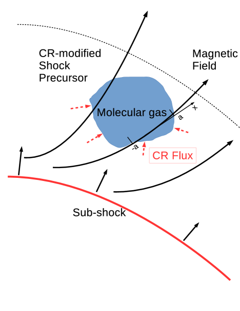
?figurename? 1: SNR shock propagating into ISM with MC upstream.

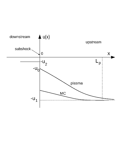
?figurename? 2: Flow profile near a CR modified shock. The line ’MC’ shows an MC trajectory on the phase plane. The speed of MC is considerably higher than that of the flow because of its inertia, resulting in a weaker slow down by the CR pressure than that for the main plasma. The drag from the plasma is also assumed to be not sufficient to slow down the MC significantly.

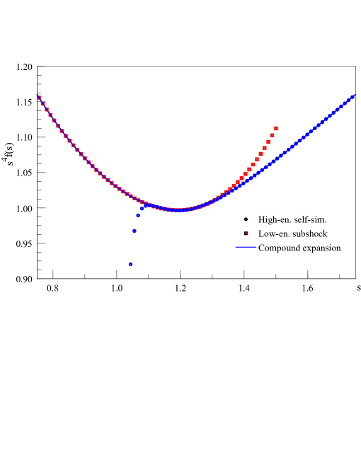
?figurename? 3: Matching of low (dashed line) and high (solid line) momentum solutions of eq.(20) given by eq.(35). An overlap region at $s\gtrsim 1$ ensures a smooth transition between the two asymptotics. They deviate from the actual solution at high/low momenta. The matched asymptotic (compound), uniformly valid solution is shown by the solid line. The matching parameters in eq.(35) are $\beta=0.95$, $B=0.05$ and $A=0.9785.$ The subshock compression, $r_{s}=3$, so $q_{s}=4.5.$

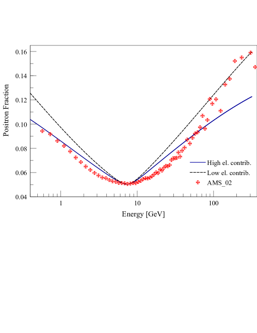
?figurename? 4: Positron fraction, represented as a ratio of $e^{+}$ spectrum to the sum of $e^{+}$ and $e^{-}$, as given in eq.(37). A fit of the AMS-02 data to the solution of eq.(20) given by eq.(35) with $\beta=0.95$, $p_{0}=6.33$, $A=0.9785$, $B=0.05$ and the mix of species represented by eq.(37) is shown for the two sets of normalization and $e^{\pm}$ mixing constants, $C$ and $\zeta$. They correspond to a high and low electron contribution to the mix, with $\zeta=9$ and $\zeta=5,$ respectively. To comply with the AMS-02 at the spectrum minimum, we fixed the normalization constant at $C=1.45$ and $C=1.25$ for these two cases.

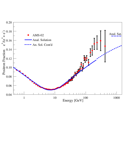
?figurename? 5: The same as Fig.4 but plotted for an averaged shock modification: instead of the specified shock modification parameter $p_{0}=6.33$ used in Fig.4, two different values of $p_{0}$ are chosen, $p_{0,1}=5.2$ and $p_{0,2}=8.0.$ Shown is the positron fraction, obtained as an average between those obtained for $p_{0}=p_{0,1}$ and $p_{0,2}$ (solid line). The dashed line extends this solution to higher energies, using a simplified calculation with a fixed value of $p_{0}\approx\left(p_{0,1}+p_{0,2}\right)/2$, because the effect of $p_{0}$ dispersion is not significant at high energies. Parameters in eq.(37) are fixed at $C=0.061$ and $\zeta=0.35$, so that the saturation level predicted by eq.(36) is $\approx 0.17$, shown in the upper right corner. AMS-02 error bars added, where they are significant ($E>30$ GeV).

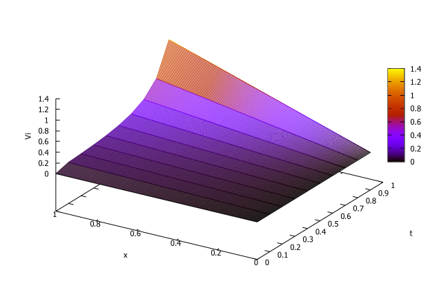
?figurename? 6: Time evolution of the ion velocity profile, starting from $V_{i}\left(x,0\right)\equiv 0$, as described by eqs.(7-8). The CR source term is prescribed according to eq.(3), $n_{CR}\propto 1/\left(t_{0}-t\right).$ The ion density remains constant in $x$ at all times. Here $x=0$ corresponds to the mid point of the MC, while $x=1$ – to its edge.