NOON States via Quantum Walk of Bound Particles

Abstract

Tight-binding lattice models allow the creation of bound composite objects which, in the strong-interacting regime, are protected against dissociation. We show that a local impurity in the lattice potential can generate a coherent split of an incoming bound particle wave-packet which consequently produces a NOON state between the endpoints. This is non trivial because when finite lattices are involved, edge-localization effects make their use for non-classical state generation and information transfer challenging. We derive an effective model to describe the propagation of bound particles in a Bose-Hubbard chain. We introduce local impurities in the lattice potential to inhibit localization effects and to split the propagating bound particle, thus enabling the generation of distant NOON states. We analyze how minimal engineering transfer schemes improve the transfer fidelity and we quantify the robustness to typical decoherence effects in optical lattice implementations. Our scheme potentially has an impact on quantum-enhanced atomic interferometry in a lattice.

I Introduction

The unprecedented ability to control and observe multi-particle states in optical lattice systems with single-site resolution weitenberg_single-spin_2011 ; preiss_strongly_2015 ; fukuhara_microscopic_2013 ; fukuhara_quantum_2013 ; murmann_two_2015 ; preiss_quantum_2015 ; robens_quantum_2015 ; celi_synthetic_2014 ; mancini_observation_2015 ; chiara_detection_2011 ; islam_measuring_2015 ; zupancic_ultra-precise_2016 ; ott_single_2016 ; hoffmann_holographic_2016 make possible the investigation of new quantum interference effects. Indeed, the dynamics of quantum interacting systems display many interesting features that go beyond the regime traditionally studied in linear optics. From the fundamental perspective it is then important to understand how to exploit the natural interactions to “engineer” the many-particle dynamics in a lattice for creating non-classical states, such as multi-particle NOON states. Compared to classical setups, and also to other schemes for atom interferometry rocco_fluorescence_2014 ; kovachy_quantum_2015 , the advantage of this approach is that non-classical states (e.g. NOON and dual Fock states lee_quantum_2002 ) enhance the estimation precision of the phase difference between the output arms of an interferometer dowling_quantum_2008 ; demkowicz-dobrzanski_chapter_2015 ; gross_nonlinear_2010 ; gross_spin_2012 , making them highly attractive for technological applications. Super-resolution for NOON states with $N=2,3$ has been recently shown experimentally for microscopy purposes israel_supersensitive_2014 . However, the generation of non-classical states with high-fidelity is still a hard task. For instance, in existing photonic realizations, NOON states with $N=5$ have been demonstrated, but with a limited $42\%$ fringe visibility hofmann_high-photon-number_2007 ; afek_high-noon_2010 ; israel_experimental_2012 . Moreover, with those schemes, there is a theoretical upper threshold for the state preparation fidelity of $94.3\%$ hofmann_high-photon-number_2007 . It is therefore important to develop alternative schemes for high-fidelity NOON states generation.

To sense spatial inhomogeneities and to probe external fields localized over few sites, it is convenient for the components of the NOON state to be spatially well separated. In this context a quantum walk of interacting atoms in an optical lattice might be very useful as we shall explore. For a lattice setup this type of scheme is important as it enables one to avoid the necessity of measurement based schemes kok_creation_2002 ; mullin_creation_2010 (which are still challenging in current optical lattice experiments with few particles), time-dependent external potentials stiebler_spatial_2011 , engineered bath based schemes kordas_dissipation-induced_2012 or ring lattices leung_dynamical_2012 ; dellanna_entanglement_2013 . From the theoretical point of view, optical lattice systems in a low filling limit are modeled by the Bose-Hubbard Hamiltonian, which contains a hopping term between neighboring sites and an onsite interaction. If more than one particles are initially located in the same site and the onsite interaction is sufficiently strong, this model favors the creation of bound states, which are stable against dissociation winkler_repulsively_2006 ; petrosyan_quantum_2007 ; folling_direct_2007 ; valiente_two-particle_2008 ; valiente_three-body_2010 ; preiss_strongly_2015 . A natural question is then whether bound states have some advantages for non-classical state production tasks. The key point here is that a bound state behaves like an effective single particle for strong enough interaction and together with a balanced beam splitter it can be used to produce a high fidelity NOON state. When distant sites are involved, a balanced beam splitter transformation can be obtained via the particle dynamics by introducing suitable impurities in the lattice potential. These impurities generate a coherent splitting of the wave-packet of propagating particles which enables high-efficiency effective linear optical operations between remote sites of finite lattices compagno_toolbox_2015 ; banchi_perfect_2015 . Even without the onsite interaction, peculiar quantum interference effects enable the production of non-classical states, namely two particle NOON states, via the celebrated Hong-Ou-Mandel effect compagno_toolbox_2015 ; banchi_perfect_2015 . Being a linear-optical effect, the efficiency of this protocol is maximized when the atom-atom interaction is kept in the weak coupling regime.

On the other hand it is intriguing to investigate the strongly interacting regime, namely whether the role of the inter-atomic interaction can be exploited as a resource to generate a wider class of non-classical states, for instance high NOON states ($N>2$) between distant sites.

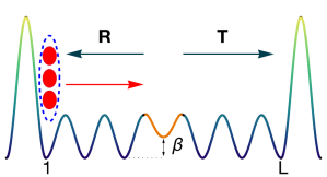
Figure 1: Scheme of the model: when a bound state is initially in the site $1$ of a finite lattice, a suitably introduced local impurity (orange) in the chemical potential $\mu_{j}=-\beta\delta_{j,L/2+1}$ triggers a wave-packet splitting in a reflected $R$ and a transmitted $T$ component. If appropriately tuned it generates a NOON state between the endpoints (site $1$ and $L$) at the transfer time. The two green peaks are local fields which realize a finite lattice model. The red arrow represents the natural direction of propagation of the bound particle once lowered the lattice depth at time $t=0$. We also add local fields in the first and last sites of the chain to inhibit the edge-localization effect and then to delocalize the bound particle from the edges.

However, as far as distant sites are concerned, the realizability of this scheme is hindered by the possibility to engender and control the tunneling dynamics of a bound state initially located in one edge of the lattice. The main obstacle is the presence of edge-locked states which inhibit the hopping dynamics pinto_edge-localized_2009 ; haque_self-similar_2010 . Edge-locking indeed creates an effective energy barrier between edge and bulk sites, that suppresses the bound state propagation along the lattice.

In other words, it is still an open problem how to tune the lattice potential to realize transformations between far sites when strongly interacting particles are involved. Recently, in the case of fermions, a long-range state transfer protocol for a two particle bound state has been studied in a one- and two-dimensional lattices, using AC fields. In this scheme the state transfer takes place only between edge states, while bulk sites remain empty during the dynamics of the system bello_long-range_2016 ; bello_sublattice_2016 . On the other hand, for bosonic particles, the under-barrier tunneling of a dimer has been analyzed in kolovsky_energetically_2012 ; maksimov_escape_2014 . Nonetheless, the problem of how to transfer bound states with high fidelity over arbitrarily long distances in engineered finite-size chains has not been completely addressed yet, in particular when more than two particle bound states are involved in the dynamics.

In this paper we analyze the bound particle dynamics in a finite lattice by mapping the Bose-Hubbard Hamiltonian into an effective single particle chain via a strong-coupling expansion in the onsite interaction term. This mapping is realized with a novel application of the effective theory developed in jia_integrated_2015 . We study the conditions to prevent the dissociation of the bound particle during the dynamics and we show that when these conditions are satisfied the bound particle evolution is perfectly described by our effective model. We find the connection between the effective hopping rates, which are interaction dependent, and the physical parameters of the of the Bose-Hubbard model. We then show how to design these parameters such that the effective evolution produces a splitting transformation suitable for creating NOON states between distant sites. Applications in quantum enhanced metrology are thus discussed.

The first step towards the realization of our protocol is to develop a method to delocalize a bound state wave-packet from the edges of a finite chain. In the spin chain case the edge-locking effect for spin blocks is bypassed using $\pi$ pulses to flip the leftmost spin and then enable the wave-packet delocalization haque_self-similar_2010 ; alba_bethe_2013 . On the other hand, in Bose-Hubbard model an operative method to unlock bound particle states has not been proposed yet. Here we show that the edge locking effect can be eliminated by introducing static impurities in the chemical potential localized at the endpoints. These impurities, which can be generated using external local fields, compensates the energy gap between edge and bulk sites and enable the dynamics. After “unlocking” the dynamics, we study the state transfer efficiency for a uniform chain and the robustness from typical environmental effects, specifically decoherence effects due to spontaneous emission in an optical lattice setup. Moreover we show how a minimal engineering of the hopping rates can enhance the transfer efficiency, specifically tuning the first and the last tunneling couplings of the chain. We show then how to add an extra impurity in the middle of the chain to generate a NOON state between the edges of the lattice. We derive analytical expressions for the optimal parameters to generate $N=2$ and $N=3$ NOON states, and we show how our approach can be straightforwardly generalized for producing larger “cat” states. Finally, we show how to experimentally detect the generated NOON state using the technology available nowadays.

II Main idea

We consider a one-dimensional chain of length $L$, described by a Bose-Hubbard model with site dependent parameters according to the following Hamiltonian lewenstein_ultracold_2012 :

$$H=-\sum\limits_{j=1}^{L-1}\frac{J_{j}}{2}\left[a_{j}a_{j+1}^{\dagger}+H.c.\right]+\sum\limits_{j=1}^{L}\frac{U_{j}}{2}n_{j}\left(n_{j}+1\right)-\sum\limits_{j=1}^{L}\mu_{j}n_{j}~{}.$$ (1)

Here $a_{j}(a_{j}^{\dagger})$ are the boson annihilation (creation) operators, $n_{j}=a_{j}^{\dagger}a_{j}$ the number operator and $J_{j}$, $U_{j}$ and $\mu_{j}$ are respectively the hopping rate, the onsite interaction and the chemical potential. Because the Hamiltonian, Eq. (1), preserves the total number of excitations of the system, the dynamics can be evaluated in a Hilbert subspace with a fixed number of particles.

One characteristic feature of the Bose-Hubbard model is that the onsite interaction enables the creation of “bound” states when several particles are in the same site winkler_repulsively_2006 ; folling_direct_2007 ; petrosyan_quantum_2007 ; valiente_two-particle_2008 ; valiente_three-body_2010 ; preiss_strongly_2015 . Here we are interested in a non-equilibrium configuration, in the low filling regime, where $M$ particles are initially located on a single site. In optical lattices the initialization of the system in one of these states is obtained starting from the Mott-Insulator regime and using single-atom addressing techniques weitenberg_single-spin_2011 ; preiss_strongly_2015 ; fukuhara_microscopic_2013 ; fukuhara_quantum_2013 ; preiss_quantum_2015 ; islam_measuring_2015 . The key point here is that, provided that the onsite interaction strength $U$ is large enough, the resulting state composed of $M>1$ bounded particles on the same site is stable against dissociation during the time evolution winkler_repulsively_2006 ; petrosyan_quantum_2007 ; valiente_two-particle_2008 ; valiente_three-body_2010 ; lahini_quantum_2012 ; qin_statistics-dependent_2014 , and behaves like an effective single particle. Indeed, as explicitly discussed in valiente_two-particle_2008 ; valiente_three-body_2010 for a few values of $M$, the bounded-particle states lie in an energy band which is well-separated (by an energy separation $\propto U$) from other states, provided that $U$ is suitably large. In the following we introduce a general theory to model the effective interactions between stable bounded particles.

In general when $U_{j}\gg J_{j},\mu_{j}$ the different Hilbert subspaces $\mathcal{H}_{M}$ spanned by the states with $M$ bounded particles, namely $\mathcal{H}_{M}=\{|{\{M\},j}\rangle{=}(a_{j}^{\dagger})^{M}|{0}\rangle/\sqrt{M!}:j{=}1,\dots,L\}$, are energetically well separated. Because of this energy separation between subspaces, if the initial state is composed of a bound $M$-particle states, then with a good approximation the dynamics remains confined inside $\mathcal{H}_{M}$. The resulting effective dynamics can be described with a Hamiltonian $H^{\rm eff}_{M}$ which describes the effective interactions inside $\mathcal{H}_{M}$. By exploiting the theory presented in jia_integrated_2015 , which assumes that the dynamical effective subspace is energetically separated by rest of the Hilbert space, we find that 1, generates in $\mathcal{H}_{M}$ the following effective interaction

$$H_{M}^{\mathrm{eff}}=\left(\begin{array}[]{ccccc}B^{\mathrm{eff}}_{1}&J^{\mathrm{eff}}_{1}&&&\\ J^{\mathrm{eff}}_{1}&B^{\mathrm{eff}}_{2}&J^{\mathrm{eff}}_{2}&&\\ &\ddots&\ddots&\ddots&\\ &&J^{\mathrm{eff}}_{L{-}2}&B^{\mathrm{eff}}_{L^{-}1}&J^{\mathrm{eff}}_{L{-}1}\\ &&&J^{\mathrm{eff}}_{L{-}1}&B^{\mathrm{eff}}_{L}\end{array}\right)$$ (2)

in the basis $|{\{M\},j}\rangle$, $j{=}1,\dots,L$. The above Hamiltonian describes a quantum walk of a one-dimensional bounded particle. We mention that, recently, using a different approach, an effective spin-chain model has been obtained to control and manipulate a 1D strongly interacting two specie Bose-Hubbard for quantum communication and computation purposes volosniev_engineering_2015 . Quantum walks have been subject to intensive investigations over the past years, both with single particles and multi-particles lahini_quantum_2012 ; qin_statistics-dependent_2014 ; preiss_strongly_2015 ; lorenzo_transfer_2015 ; apollaro_many-qubit_2015 ; sousa_pretty_2014 ; paganelli_routing_2013 . In particular, different schemes have been found to engineer the couplings $J^{\rm eff}_{j}$ and the energies $B^{\rm eff}_{j}$ such that the dynamics either produces a perfect state transfer christandl_perfect_2004 ; kostak_perfect_2007 ; kay_perfect_2010 or a perfect splitting and reconstruction of the initial wave-packet, namely a fractional revival banchi_perfect_2015 ; genest_quantum_2015 ; lemay_novel_2015 . From our perspective, a perfect state transfer in the effective subspace would give rise to a perfect transmission of a bounded particle: namely the state $|{\{M\},1}\rangle\propto(a_{1}^{\dagger})^{M}|{0}\rangle$ is dynamically transferred to the opposite end of the chain $|{\{M\},L}\rangle\propto(a_{L}^{\dagger})^{M}|{0}\rangle$. Another important application is the perfect fractional revival, which effectively generates a beam splitting transformation between the ends of the chain. The main reason for its importance is that when bound states are involved in the perfect splitting transformation, $|{\{M\},1}\rangle\to|{\{M\},1}\rangle+e^{i\phi}|{\{M\},L}\rangle$, then a $M$-particle NOON state $[(a_{1}^{\dagger})^{M}+e^{i\phi}(a_{L}^{\dagger})^{M}]|{0}\rangle$ is produced.

The main idea of our scheme is then to engineer the couplings $J_{j}$ and the chemical potentials $\mu_{j}$ in the Bose-Hubbard, Eq. (1), such that the effective couplings in Eq. (2) have the suitable pattern for either state transfer or state splitting (fractional revival). The time scale the resulting effective dynamical transformation is approximately given by $1/J_{\rm eff}$. However, since the effective hopping in $\mathcal{H}_{M}$ involves $M-1$ “virtual” transitions through states which are outside $\mathcal{H}_{M}$, then it is simple to realize that $J^{\rm eff}_{j}\propto J_{j}^{M}/U_{j}^{M-1}$, so $J^{\rm eff}_{j}$ exponentially decreases with $M$ for large $U$. For larger $M$-particle bound states the effective evolution thus become slow and the efficiency of the scheme may be severely affected by environmental effects. Because of this, in the next sections we thoroughly analyze the $M=2$ and $M=3$ cases which are more feasible, given the current experimental capabilities. The overall theoretical scheme is however fully general and can be readily extended for larger values of $M$.

III Applications

III.1 Edge unlocking

Before focusing on the specific $M=2$ and $M=3$ cases, we start by discussing some general properties of the quantum walk of bounded particles, to clarify the differences with the single particle counterpart. We consider the uniform coupling regime, namely $J_{j}=J$, $U_{j}=U$, $\mu_{j}=\mu$, in the initial state $|{\{M\},1}\rangle\propto\left(a_{1}^{\dagger}\right)^{M}|{0}\rangle$. The resulting effective interaction is

$$H_{M}^{\mathrm{eff}}=\left(\frac{J}{U}\right)^{M-1}\left(\begin{array}[]{ccccc}B^{\mathrm{eff}}_{1}&J^{\mathrm{eff}}_{1}&&&\\ J^{\mathrm{eff}}&B^{\mathrm{eff}}_{2}&J^{\mathrm{eff}}&&\\ &\ddots&\ddots&\ddots&\\ &&J^{\mathrm{eff}}&B^{\mathrm{eff}}_{L^{-}1}&J^{\mathrm{eff}}\\ &&&J^{\mathrm{eff}}&B^{\mathrm{eff}}_{L}\end{array}\right)$$ (3)

where $J^{\rm eff}=\mathcal{O}(J)$, $B_{1}^{\rm eff}=B_{L}^{\rm eff}=\mathcal{O}[J(U/J)^{M-2}]$ while $B_{j}^{\rm eff}$ for $j\neq 1,L$ is much smaller than $B_{1}^{\rm eff}$ (boundary elements may be of order $\mathcal{O}(J)$ or less while in the bulk they are even smaller). The appearance of a larger effective field in the boundaries gives rise to a phenomenon which is called edge-locking. Edge-locked states, which have been already described in haque_self-similar_2010 ; pinto_edge-localized_2009 for $M\geq 3$, can be understood using the theory of quasi-uniform tridiagonal matrices banchi_spectral_2013 . To describe this phenomenon we consider an initial wave-packet localized in site 1 which evolves through the Hamiltonian, Eq. (3), to the wave-packet $|{\psi(t)}\rangle=\sum_{j}(e^{-itH_{M}^{\rm eff}})_{j1}|{\{M\},j}\rangle$. Calling $H_{M}^{\rm eff}=VEV^{\dagger}$ the spectral decomposition of the effective Hamiltonian, then $|{\psi(t)}\rangle=\sum_{kj}e^{-itE_{k}}V_{1k}V^{*}_{jk}|{\{M\},j}\rangle$. Because of the mirror symmetry and for the properties of quasi-uniform matrices banchi_spectral_2013 one finds that $V_{Lk}=V_{1k}(-1)^{k}\approx V_{1k}e^{iLk}$ and $E_{k}\propto\cos(k)$ where $k$ is the quasi-momentum, $k=k_{j}+\mathcal{O}(L^{-1})$ where $k_{j}=\pi j/(L+1)$ and $j=1,\dots,L$. Therefore the quantum walk of the bounded particle displays the standard expression of a wave-packet evolution banchi_long_2011 , as $\langle{\{M\},L}|{\psi(t)}\rangle=\sum_{k}e^{-i(tE_{k}-Lk)}|V_{1k}|^{2}$ where $|V_{1k}|^{2}$ is the probability to excite the quasi-momentum state $k$ by initializing the system in the first site. To simplify the theoretical analysis we assume that $B_{j}^{\rm eff}\equiv B_{\rm bulk}^{\rm eff}$ is constant for $j\neq 1,L$ so, without loss of generality, we can set $B_{\rm bulk}^{\rm eff}=0$. Indeed, the Hamiltonian (3) and $H^{\rm eff}_{M}-B_{\rm bulk}^{\rm eff}\mathbf{1}$ give rise to the same evolution aside from an irrelevant global phase. Within this description it is now clear that edge-locking appears when $B_{1}^{\rm eff}\gg E_{k}$, since no quasi-momentum state can be excited by initializing the system in a state where the bounded particle is in the first site (namely $|V_{1k}|^{2}\approx 0$ for all the quasi-momentum states). Indeed, in this regime this initialization excites out-of-band modes which are localized near the edges and do not propagate. As it is clear from Eq. (3), since $B_{1}^{\rm eff}=B_{L}^{\rm eff}=\mathcal{O}[J(U/J)^{M-2}]$, the edge-locking condition $B_{1}^{\rm eff}\gg E_{k}$ happens when $M\geq 3$, as obtained also in pinto_edge-localized_2009 . However, there is another form of quasi-locking for $M=2$ which is not described in pinto_edge-localized_2009 . Indeed, for $M=2$ we find that $B_{1}^{\rm eff}$ is of the same order of the energy band $E_{k}$ of the quasi-momentum states and, as a consequence, the quasi-momentum states with energy $B_{1}^{\rm eff}\approx E_{k}$ are the ones involved by the dynamics. Since $E_{k}\propto\cos(k)$ when $B_{1}^{\rm eff}\approx 0$ the relevant excitations consist mostly of quasi-momentum states with almost-linear dispersion relation ($E_{k}\approx k$ around $k=\pi/2$ where $E_{\pi/2}\simeq 0$). These states propagate without dispersion in the chain and therefore give rise to a high transmission quality. On the other hand, if $B_{1}^{\rm eff}\neq 0$ other states with non-linear dispersion relation are involved, which drastically lower the transmission quality. Because of this, we find that the state $|{\psi}\rangle{=}(a^{\dagger})^{2}|{0}\rangle$ has a long delocalization time from the initial site during the relevant time $t^{*}\sim LU/J^{2}$.

Because edge localization is detrimental in quantum transfer applications, we analyze the possibility to “unlock” the states by compensating the energy gap between edge and bulk sites introducing a local static potential both in the first and the last site of the chain. Edge unlocking can be always obtained for any value of $M$ by adding suitable local chemical potentials $\mu_{j}$ around the edges such that the effective fields $B_{n}^{\rm eff}$ are constant over the different sites $n$.

III.2 Two Particles

In this section we analyze the dynamical behavior of a two particle bound state. We first start from the uniform case, describe the edge unlocking and then we consider how to engineer the couplings to maximize the transfer of a bound state and the generation of a NOON state.

III.2.1 Edge Unlocking

For a uniform chain $J_{j}=J$, $U_{j}=U$, $\mu_{j}=\mu$ we find that the effective hamiltonian $H_{\mathrm{eff}}$ is the tridiagonal matrix in Eq. (2) where

$$J^{\rm eff}_{j}=\frac{J^{2}}{2U}~{},$$ (4)

$$B^{\rm eff}_{j}=\left\{\begin{array}[]{l@{\quad}cl}\frac{J^{2}}{2U}+U~{},&{\rm for}&j=1,L~{},\\ \frac{J^{2}}{U}+U~{},&{\rm for}&j\neq 1,L~{}.\end{array}\right.$$ (5)

The effect of the inhomogeneities in $B_{j}^{\rm eff}$ is shown in Fig. 2 (top), where we analyze the dynamics of a bound particle initially in $|{\psi(0)}\rangle\propto\left(a_{1}^{\dagger}\right)^{2}|{0}\rangle$ in a uniform chain with $L=5$ and $U/J=5$. We study the probability $P_{ij}(t)$ that after the time $t$ one particle is in the site $i$ and the other is in the site $j$, namely $P_{ij}=\frac{1}{1+\delta_{ij}}|\langle{0}|a_{i}a_{j}|{\psi(t)}\rangle|^{2}$, where $|{\psi(t)}\rangle$ is the state evolved for a time $t$. In particular we plot , as a function of the time $t$, the probability to have the bound particle in the first site $P_{11}(t)$ and in the last site of the chain $P_{LL}(t)$. We observe that despite the bound particle reaches the last site of the chain at the transfer time $t^{*}\sim L/J_{\textrm{eff}}$, the probability to be in the first site $P_{11}(t^{*})$ is still not zero, namely the delocalization time from the first site is slow compared to the transfer time $t^{*}$. As described in the previous section, this is due to the difference in effective energies $B^{\rm eff}_{j}$ between the bulk and the edges which favors non-linear excitations which, in turn, leads to a dispersive dynamics. This difference between the bulk and the edges can be made zero by adding two local chemical potentials at the endpoints, $\mu_{j}=-\beta^{\prime}\left(\delta_{j,1}+\delta_{j,L}\right)$, where $\beta^{\prime}=J^{2}/4U$. As it can be seen in Fig. 2 (bottom), when the $\beta^{\prime}$ field is added, the delocalization time from the first time $P_{11}(t^{*})$ (and consequently the transfer fidelity $P_{LL}(t^{*})$) is strongly increased. We compare the results obtained for the transfer of a bound state with the propagation of a single particle in the lattice, initially in $a_{1}^{\dagger}|{0}\rangle$, by plotting in Fig. 2 (bottom) the probability $P_{L}(t)=|\langle 0|a_{L}|\psi(t)|^{2}$ (single particle data are scaled for their transfer time $t^{*}\sim L/J$). The difference between the single particle and the bound particle results depends on the finite value of the interaction chosen ($U/J=5$ in Fig. 2). Indeed the agreements with a single particle behavior is very high as long as $U/J$ is large enough.

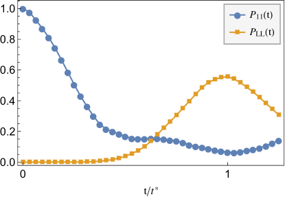
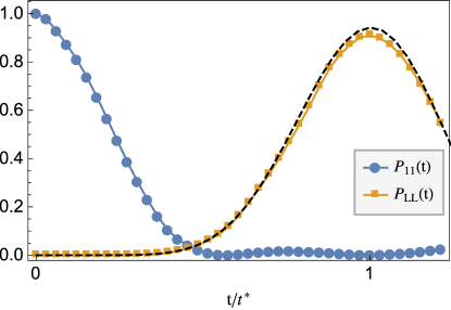
Figure 2: Edge delocalization for a two particle bound state: plot of the probability to have a bound particle in the first $P_{11}(t)$ and in the last $P_{LL}(t)$ site as a function of the time $t$, scaled for the transfer time $t^{*}\sim L/J_{\textrm{eff}}$ for a uniform chain with $L=5$ and $U/J=5$ in the initial state $|{\psi(0)}\rangle\propto(a_{1}^{\dagger})^{2}|{0}\rangle$. We add a local field $\mu_{j}=-\beta^{\prime}(\delta_{j,1}+\delta_{j,L})$ with strength $\beta^{\prime}=0$ (top), and $\beta^{\prime}=\beta_{\mathrm{opt}}^{\prime}=J^{2}/4U$ (bottom). To compare the results with the single particle case we plot, with a dashed black line, the probability $P_{L}(t)=|\langle 0|a_{L}|\psi(t)|^{2}$ for a single particle initially in $a_{1}^{\dagger}|{0}\rangle$ (here $t^{*}\sim L/J$).

Because the effective model in Eq. (2) is valid in the regime $U/J\gg 1$, we analyze deviations from the theoretical value of $\beta^{\prime}$, by evaluating the dynamics with exact diagonalization techniques as in compagno_toolbox_2015 ; banchi_perfect_2015 . Once initialized the system in $|{\psi(0)}\rangle\propto(a_{1}^{\dagger})^{2}|{0}\rangle$ we numerically find the value of $\beta^{\prime}$ that maximize the probability to find, at the transfer time $t^{*}\sim L/J_{\mathrm{eff}}$, the bound particle in the last site of the chain $P_{LL}(t^{*})$. We numerically find that, for a two particle bound state, the optimal values of $\beta^{\prime}$ completely agree with the theoretical model $\beta^{\prime}=J^{2}/4U$ independently from the length of the chain, as long as $U/J\gtrsim 5$.

When the hopping term $J$ and the onsite interaction $U$ have comparable amplitude, both the bound states and the single particle states contribute to the dynamics preiss_strongly_2015 . We expect that by increasing the onsite interaction the effects of the free particle states are reduced while the state transfer fidelity of a bound particle should converge to a constant value.

By analyzing $P_{LL}(t^{*})$ we find that, when the optimal value for the localized field $\beta^{\prime}=J^{2}/4U$ is added in a uniform chain, values of the onsite interaction above $U/J\gtrsim 4$ guarantee an almost constant value of transfer fidelity for a two particle bound state.

III.2.2 Optimal State Transfer of a Two Particle Bound state

The state transfer efficiency of a two particle bound state in a uniform chain can be improved by suitably tuning the tunneling couplings in the model in Eq. (1). Because a full engineering could be too demanding, here we consider the effect of a minimal engineering scheme banchi_long_2011 ; apollaro_99$$-fidelity_2012 , which consists of tuning the first and the last tunneling terms to $J_{1}=J_{L-1}=J_{0}$ while the rest of the chain has uniform couplings $J_{j}=J$. In this case the effective Hamiltonian (2) has effective interactions

$$J^{\rm eff}_{j}=\left\{\begin{array}[]{l@{\quad}cl}\frac{J_{0}^{2}}{2U}&{\rm for}&j=1,L-1~{},\\ \frac{J^{2}}{2U}&{\rm for}&j\neq 1,L-1~{},\end{array}\right.$$ (6)

$$B^{\rm eff}_{j}=\left\{\begin{array}[]{l@{\quad}cl}\frac{J_{0}^{2}}{2U}+U&\mathrm{for}&j=1,L,\\ \frac{J_{0}^{2}}{2U}+\frac{J^{2}}{2U}+U&\mathrm{for}&j=2,L-1,\\ \frac{J^{2}}{U}+U&{\rm for}&j=3,\dots,L-2.\end{array}\right.$$ (7)

To maximize the transfer fidelity one has then to remove the difference between the effective energies $B^{\rm eff}_{j}$, and to optimize the values of $J^{\rm eff}_{j}$ to achieve an optimal ballistic dynamics. Since the dynamics occurs in the effective subspace one can use the analytical theory presented in banchi_long_2011 to find the optimal value of $J_{0}^{\rm eff}\equiv\frac{J_{0}^{2}}{2U}$, given that the rest of the sites are coupled with a hopping strength $J^{\rm eff}\equiv\frac{J^{2}}{2U}$. Given the simple relationship between $J_{0}^{\rm eff}$ and the strength $J_{0}$ of the Bose-Hubbard tunneling between the edges and the bulk, it is then straightforward to obtain $J_{0}$. Once $J_{0}$ is found, one needs to add local chemical potentials in both the first and the last two sites to remove the local energy difference in $B^{\rm eff}_{j}$. By using our effective Hamiltonian expansion, we find that the state transfer is maximized by introducing two pairs of local fields, respectively $\mu_{j}=-\beta_{1}(\delta_{j,1}+\delta_{j,L})$ and $\mu_{j}=-\beta_{2}(\delta_{j,2}+\delta_{j,L-1})$, with strengths $\beta_{1}=\left(J_{0}^{2}-2J^{2}\right)/2U$ and $\beta_{2}=\left(J_{0}^{2}-J^{2}\right)/2U$. In Fig. 3 (top) we show the results obtained for the transfer fidelity $P_{LL}(t^{*})$ as a function of $U/J$ when we use minimal engineering and the compensating fields $\beta_{1}$ and $\beta_{2}$. We observe a significant improvement of transfer fidelity compared to the results for a uniform chain. In Fig. 3 (bottom) we also highlight the difference between the single-particle dynamics and the bound-particle case for finite interaction $U$. As expected, for strong inter-particle interaction $U$, a bound state behaves as a single particle state. To highlight that minimal engineered schemes already have a significant impact in reducing the dispersion in the system, in Fig. 3 (bottom) we show the dynamics of a bound state in a lattice. Specifically, we plot the probability $P_{jj}(t)=|\langle 0|a_{j}^{2}|\psi(t)\rangle|^{2}/2$ to have a two particle bound state in site $j$ as a function of the time $t/t^{*}$, for a minimal engineered chain with $L=21$ and $U/J=8$.

In analog fashion the Bose-Hubbard Hamiltonian couplings can be tuned so that the effective Hamiltonian coincides with the one allowing perfect state transfer christandl_perfect_2004 , though this is much more demanding because it requires the engineering of all tunneling rates $J_{j}$ and all the chemical potentials $\mu_{j}$.

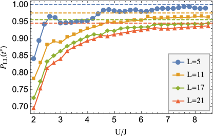
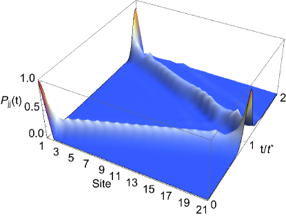
Figure 3: Optimal transfer of a two particle bound state: (top) analysis of the transfer fidelity $P_{LL}(t^{*})$ for the initial state $|{\psi(0)}\rangle\propto(a_{1}^{\dagger})^{2}|{0}\rangle$ as a function of the onsite interaction $U/J$ when the optimal transfer scheme $J_{1}=J_{L}=J_{0}$ and $J_{j}=J$ for $j\neq(1,L)$ is included in the model 1. Here we also add two local impurities $\mu_{j}=-\beta_{1}(\delta_{j,1}+\delta_{j,L})$ and $\mu_{j}=-\beta_{2}(\delta_{j,2}+\delta_{j,L-1})$ where $\beta_{1}=\left(J_{0}^{2}-2J^{2}\right)/2U$ and $\beta_{2}=\left(J_{0}^{2}-J^{2}\right)/2U$ to eliminate the edge-locking effect. The $J_{0}$ value is chosen by numerically maximizing the transfer fidelity in a single particle manifold banchi_long_2011 . To compare the difference between a single particle and a bound state, we plot (with a dashed line) also the single-particle transfer fidelity $P_{L}(t^{*})=|\langle 0|a_{L}|\psi(t^{*})\rangle|^{2}$ obtained for a system initially in $a_{1}^{\dagger}|{0}\rangle$. (bottom) Probability $P_{jj}(t)$ to have a two particle bound state in site $j$ at time $t/t^{*}$ for a minimal engineered chain with $L=21$ and $U/J=8$.

III.2.3 Environmental effects

State transfer schemes are generally robust against static imperfections in the couplings zwick_robustness_2011 ; pavlis_evaluation_2016 . On the other hand, we explicitly test the robustness of our scheme against dynamical environmental effect, specifically dephasing due to spontaneous emission, which represents the main source of decoherence in optical lattices. The dynamics of the system in the lowest band is typically modeled as a Master equation in Lindblad form kordas_non-equilibrium_2015 ; pichler_nonequilibrium_2010 ; sarkar_light_2014 :

$$\dot{\rho}=-i\left[H_{BH},\rho\right]+\Gamma\sum\limits_{i}\left(n_{i}\rho n_{i}-\frac{1}{2}n_{i}n_{i}\rho-\frac{1}{2}\rho n_{i}n_{i}\right).$$ (8)

Here $\Gamma$ is the effective scattering rate, and $H_{\mathrm{BS}}$ is the Bose-Hubbard Hamiltonian 1. We numerically solve Eq. (8) as shown in detail in C.

No relevant edge field optimal strength $\beta^{\prime}$ deviations are found when decoherence effects are introduced, for $\Gamma/J_{\mathrm{eff}}<0.1$, where $J_{\mathrm{eff}}=J^{2}/2U$. In Fig. 4 (top) we show how the transfer fidelity $P_{LL}(t^{*})$ is affected as a function of the damping rate $\Gamma/J_{\mathrm{eff}}$ in Eq. (8) for $U/J=3$.

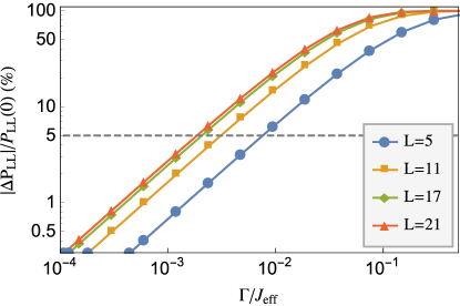
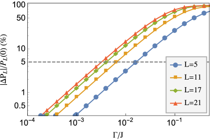
Figure 4: Decoherence effects for a two particle bound state: (top) relative variation $\Delta P_{LL}/P_{LL}(t^{*},\Gamma=0)$ of the transfer fidelity $P_{LL}(t^{*})$ with respect to the case in absence of decoherence, for a uniform chain with $U/J=3$ and length $L$. Here $\Delta P_{LL}=|P_{LL}(t^{*},\Gamma)-P_{LL}(t^{*},\Gamma=0)|$ and the dashed grey line is a threshold of a relative variation of the $5\%$. Several chain length $L$ are considered. (bottom) Relative variation $\Delta P_{L}/P_{L}(t^{*},\Gamma=0)$ for a single particle state initially in $a_{1}^{\dagger}|{0}\rangle$.

To better evaluate the difference with the zero decoherence case, we show in Fig. 4 the relative variation $|\Delta P_{LL}(t^{*})|/P_{LL}(0)=|P_{LL}(\Gamma)-P_{LL}(\Gamma=0)|/P_{LL}(\Gamma=0)$ with respect to the no decoherence case, as a function of the damping parameter $\Gamma/J_{\mathrm{eff}}$. We observe deviations of less than the $5\%$ for $\Gamma/J_{\mathrm{eff}}\simeq 10^{-2}-10^{-3}$ for chain lengths between $L\in\left\{5,\ldots,21\right\}$ which are typical values for blue detuned optical lattices sarkar_light_2014 ; pichler_nonequilibrium_2010 . In Fig. 4 (bottom) we show the effects of the decoherence in the state transfer fidelity for a single particle state, initially in $a_{1}^{\dagger}|{0}\rangle$.

III.2.4 NOON State Generation with a Two Particle bound state

In this section we consider an imperfect fractional revival by considering a uniform evolution, though the present results can be extended with a further engineering to achieve perfect fractional revivals.

We consider the simplest scheme where the wave-packet splitting is achieved by using a local barrier in the middle of the chain, as shown in Fig. 1 and discussed in compagno_toolbox_2015 . We set the value $\beta^{\prime}=J^{2}/4U$ for the edge fields $\mu_{j}=-\beta^{\prime}(\delta_{j,1}+\delta_{j,L})$ to remove edge locking. Then we add a local field in the middle of the chain $\mu_{j}=-\beta\delta_{j,L/2+1}$ to trigger a wave-packet splitting compagno_toolbox_2015 . Indeed, the extra barrier favors the splitting of the propagating bound particle wave-packet into a transmitted and reflected component. It has been shown in compagno_toolbox_2015 that for single particle quantum walk, the optimal 50/50 splitting is obtained when the strength $\beta$ of this extra barrier is equal to the hopping rate. We expect that when the bound particle impinges the splitting field because it behaves like an effective single particle, the output state, measured at the endpoints, will be $|{\psi(t^{*})}\rangle_{1L}=\frac{1}{\sqrt{2}}\left(|{2,0}\rangle+i|{0,2}\rangle\right)$, namely we generate a NOON state with two particles (here $|{2}\rangle=(a^{\dagger})^{2}|{0}\rangle/\sqrt{2}$). On the other hand if the two particles are non interacting $U/J=0$, the effect of the splitting field is to produce also a non-zero probability $P_{1L}(t^{*})$ to have one particle in each end laloe_quantum_2011 . We show, for a $L=5$ chain with $U/J=5$ in Fig. 5 that for a bound particle that term is suppressed at the transfer time $t^{*}$, as expected from a bound particle effective evolution.

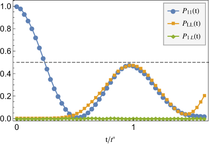
Figure 5: Two particle NOON state: plot of the probabilities $P_{ij}(t)$ to have one particle in site $i$ and the other in $j$, as a function of the time, in unit of the transfer time $t^{*}$, for two particles initially in $|{\psi(0)}\rangle\propto\left(a_{1}^{\dagger}\right)|{0}\rangle$. Here we consider a uniform chain with an impurity $\mu_{j}=-\beta\delta_{j,L/2+1}$ where $\beta=0.789(J^{2}/2U)$ in a a chain with $U/J=5$ and length $L=5$. The absence of the $P_{1L}(t^{*})$ term is an evidence that the output state at $t=t^{*}\simeq UL/J^{2}$ is the NOON state with two particles. The grey dashed line represents the results for an ideal lossless NOON state generation.

Therefore we can conclude that the output state is, when $U$ is large enough, the NOON state with two particles, apart from a damping factor due to dispersion. By performing an effective Hamiltonian expansion in the onsite interaction term we show that to have a balanced splitting in the effective space, the strength of the splitting field in the real chain must be $\beta=\beta^{50/50}=J^{2}/2U$, in the limit $L\gg 1$.

Finite length corrections are found numerically by finding the $\beta$ value for which the difference $P_{11}(t^{*})-P_{LL}(t^{*})$ is zero. As shown in the inset in Fig. 6, for a $L=5$ uniform chain, $\beta^{50/50}$ scales as $1/U$. The finite length factors, found from a fit over the data for several chain lengths, are shown in Fig. 6. By increasing the chain length $L$ the $\beta^{50/50}$ values are closer to $0.5J^{2}/U$ in agreement with the effective Hamiltonian analysis.

Figure 6: Finite-size effects in the two particle NOON state generation: analysis of the scaling factor $\alpha$ where $\beta^{50/50}=\alpha J^{2}/U$, as a function of the chain length $L$ for generating a two particle NOON state. The grey line represents the theoretical results from the effective Hamiltonian theory, which holds for $L\gg 1$. (Inset) Analysis of the optimal value of $\beta$ of the local field $\mu_{j}=-\beta\delta_{j,L/2+1}$ which produces the NOON state with two particles as a function of $U/J$ for $L=5$. The red line is the fit $\beta=\beta^{50/50}=0.395J^{2}/U$.

We underline that the NOON state creation efficiency can be made arbitrarily close to 100% by tuning the couplings in the effective bound particle subspace using the techniques for perfect splitting developed in banchi_perfect_2015 ; genest_quantum_2015 which require a complete engineering of the couplings in the Hamiltonian (1). In Section IV we propose two methods for detecting the NOON state generated by measuring interference fringes.

III.2.5 Even Chains

Here we clarify that our scheme is not limited to odd length chains but also can be applied to even chains by tuning both the middle tunneling coupling strength $J_{L/2}$, and adding two pairs of local fields, respectively $\mu_{j}=-\beta_{1}(\delta_{j,1}+\delta_{j,L})$ and $\mu_{j}=-\beta_{2}(\delta_{j,2}+\delta_{j,L-1})$ in the Hamiltonian (1). Using the results in compagno_toolbox_2015 for the splitting of a single particle we find, from the effective Hamiltonian model, that the optimal coupling strengths to generate a two particle NOON state between the endpoints of a uniform chain are respectively $J_{L/2}=J(\sqrt{2}-1)^{1/2}$, $\beta_{1}=J/4U$ and $\beta_{2}=J(2-\sqrt{2})/4U$.

III.3 Three Particles

The extension of the previous scheme to more than two particle bound states enhances its non-classical state generation capabilities, namely towards realizing small cat states between remote sites. As before the onsite interaction generates bound states with three particles when initially located in the same site. Similarly to the two particle case, one would expect that the results of the splitting process, when the onsite interaction is strong enough, is to produce a NOON state with $N=3$.

As for the two-particle case, for large onsite interactions the effective evolution in the bound particle subspace is described by Eq. (2). We consider a uniform chain, while a minimally engineered model is discussed in B. For a uniform chain the effective hopping is $J_{\mathrm{eff}}=3J^{3}/16U^{2}$. Moreover, to remove edge locking and compensate the energy gap between the endpoint sites and the bulk of the chain we have to introduce two local fields $\mu_{j}=-\beta^{\prime}\left(\delta_{j,1}+\delta_{j,L}\right)$. From our expansion we find for a uniform chain that $\beta^{\prime}=J^{2}/8U$. To check for finite-size correction to the above analytical prediction we numerically analyze the value of $\beta^{\prime}$ for several chain length $L$ for the initial state $|{\psi(0)}\rangle\propto\left(a_{1}^{\dagger}\right)^{3}|{0}\rangle$ as a function of the onsite interaction $U$. We find that with high accuracy the estimated field $\beta^{\prime}=J^{2}/8U$ is independent on $L$. We analyze the probability $P_{LLL}(t^{*})$ to have three particles in the site $L$ after time $t^{*}$ for a uniform chain as a function of the onsite interaction. We find that values of the onsite interaction above $U/J\gtrsim 4$ guarantee an almost constant value of transfer fidelity for chain lengths $L\in\left\{5,\ldots,21\right\}$.

In Fig. 7 we show the effect of decoherence due to spontaneous emission, Eq. (8) for several chain lengths $L$ as a function of the decoherence rate $\Gamma/J_{\mathrm{eff}}$ where $J_{\mathrm{eff}}=3J^{3}/16U^{2}$. We observe relative variation of less than the $5\%$ with respect to the decoherence free case, for $\Gamma/J_{\mathrm{eff}}\lesssim 1.3\times 10^{-4}$ up to $L=7$ sites.

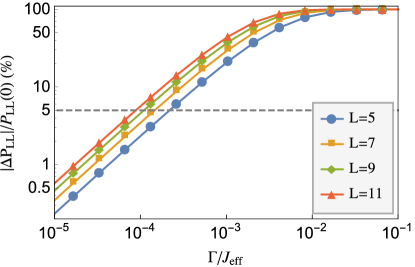
Figure 7: Decoherence effects for a three particle bound state: relative variation $\Delta P_{LL}/P_{LL}(t^{*},\Gamma=0)$, with respect to decoherence free case, for a uniform chain with $U/J=2$. Here $\Delta P_{LL}=|P_{LL}(t^{*},\Gamma)-P_{LL}(t^{*},\Gamma=0)|$ and the dashed grey line is a threshold of a relative variation of the $5\%$. Several chain length $L$ are considered.

The state transmission fidelity of a three bound particle state can be optimized by engineering the end tunneling couplings of the chain, as shown in B. In this case to bypass the edge-localization effects we also need to add a local chemical potential tuning in the first two and last two sites of the chain.

III.3.1 NOON State generation for a three particle bound state

In the non-interacting case $U/J=0$ when three particles are initially located in the first site $|{\psi(0)}\rangle\propto(a_{1}^{\dagger})^{3}|{0}\rangle$ an ideal beam splitter transformation generates as output a state with probabilities laloe_quantum_2011 : $P_{111}=P_{LLL}=1/8,\ P_{1LL}=P_{11L}=3/8$ where we define $P_{jkl}(t)=\frac{|\langle 0|a_{i}a_{j}a_{k}|\psi(t)\rangle|^{2}}{1+\delta_{ij}+\delta_{jk}+\delta_{ik}+2\delta_{ij}\delta_{jk}}$ the probability to have the three particles in the sites $i,j,k$. We expect that when the onsite interaction is strong enough, the bound particle behaves as an effective single bound particle, thus the terms $P_{1LL},P_{11L}$ are suppressed and the output state at the end points effectively results in the NOON state $|{\psi(t^{*})}\rangle_{1L}=\frac{1}{\sqrt{2}}\left(|{3,0}\rangle+i|{0,3}\rangle\right)$, where $|{3}\rangle=(a^{\dagger})^{3}|{0}\rangle/\sqrt{6}$. In Fig. 8 we plot, as a function of time (in $t^{*}\simeq L/J_{\mathrm{eff}}$ units) the probability to have a three particle bound state respectively, in the first site $P_{111}(t)$, in the last $P_{LLL}(t)$ and one particle in the first site and two in the last $P_{1LL}(t)$ in a uniform chain with $U/J=5$ and $L=5$. Here we set the edge fields strength to $\beta^{\prime}=J^{2}/8U$ and we find numerically that the splitting field to have a balanced splitting is $\beta=\beta^{50/50}=0.099J^{3}/U^{2}$. The absence of the term $P_{1LL}(t^{*})=P_{11L}(t^{*})$ is an evidence that a NOON state with three particle is generated between the edges of the chain.

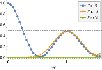
Figure 8: Three particle NOON state: joint probabilities $P_{ijk}(t)$ as a function of the time, in unit of the transfer time $t^{*}$, for three particles initially in $|{\psi(0)}\rangle\propto\left(a_{1}^{\dagger}\right)|{0}\rangle$ for a uniform chain with an impurity $\beta=0.099J^{3}/U^{2}$ and $\beta^{\prime}=J^{2}/8U$in the middle of the chain with $U/J=5$ and length $L=5$. The absence of the $P_{1LL}(t)$ term is an evidence that the output state at $t=t^{*}$ is the NOON state with two particles. The grey dashed line represents the results for an ideal lossless NOON state generation. We found also that $P_{1LL}(t)=P_{11L}(t)$.

From the effective Hamiltonian description we find that to generate a balanced splitting of a bound three particle wave-packet, we need to add a local field $\mu_{j}=-\beta^{50/50}\delta_{j,L/2+1}$ whose strength, when $L\gg 1$, is $\beta^{50/50}=J^{3}/8U^{2}$ (as explained in appendix $B$). However, finite size corrections change the value of $\beta^{50/50}$, and by performing a numerical fit over the data for a uniform chain with $L=5$ (whose results are shown in the inset of Fig. 9), we find that $\beta^{50/50}$ scales with the onsite interaction as $\beta^{50/50}=\alpha J^{3}/U^{2}$ where $\alpha\simeq 0.099$. Deviations from the theoretical value of $\beta^{50/50}=J^{3}/8U^{2}$, which are shown in Fig. 9, have been found by analyzing the results obtained for several chain length $L$. Here the dashed grey line represents the theoretical value of the coefficient $\alpha$ of the splitting field for $L\gg 1$.

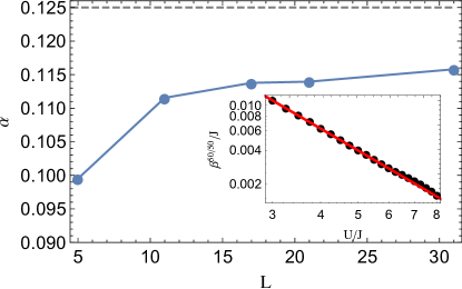
Figure 9: Finite-size effects in the three particle NOON state generation: analysis of the scaling factor $\alpha$ as a function of the chain length $L$ for a three particle bound state, where $\beta^{50/50}=\alpha J^{3}/U^{2}$. The dashed grey line represents the theoretical value from the effective Hamiltonian description. (Inset) Analysis of the optimal value of $\beta$ to produce the NOON state with three particles as a function of $U/J$ in a uniform chain with length $L=5$. The red line is the fit $\beta^{50/50}=\alpha J^{3}/U^{2}$ where $\alpha=0.099$.

IV NOON State Verification

The creation and the detection of a NOON state can be revealed by measuring the interference fringes in a Mach-Zehnder setup. After initializing the bound particles in the initial state $|{\psi(0)}\rangle\propto\left(a_{1}^{\dagger}\right)^{N}|{0}\rangle$, the NOON state is generated by the splitting field in the middle of the chain, as previously discussed. By freezing the dynamics of the system at the transfer time $t^{*}$, a controllable phase factor can be added using a local field in the last site of the chain. Finally, once lowered the lattice potential, a second beam splitter operation is performed by the splitting field which produces interference fringes at the endpoints of the chain at $2t^{*}$.

For an ideal lossless transformation the state at the two boundary sites of the chain at the transfer time $t^{*}$ would be

$$|{\psi(t^{*})}\rangle_{1L}=\frac{1}{\sqrt{2}}\left(|{N0}\rangle+i|{0N}\rangle\right)~{}.$$ (9)

Once we apply the phase transformation $\Phi=\mathrm{diag}(1,e^{i\phi})$ (namely a phase shift on site $L$), a second ideal beam splitting transformation would produce the output state at time $2t^{*}$:

$$|{\psi(2t^{*})}\rangle_{1L}=\frac{1}{2}\left[\left(1-e^{iN\phi}\right)|{N0}\rangle+i\left(1+e^{iN\phi}\right)|{0N}\rangle\right]~{},$$ (10)

where the phase accumulated is $N\phi$ with $N$ being the number of particle in the NOON state. Therefore the presence of a NOON state is revealed by measuring the interference fringes (i.e. the probability to have $N$ particle in the first site as a function of $\phi$). Although previous experimental results measured just the parity of single sites (which would exclude a direct observation of the $N=2$ case discussed so far), this detection issue in optical lattice has been recently circumvented up to four particles in the same site zupancic_ultra-precise_2016 .

We evaluate numerically the interference fringes for a two particle bound state in a uniform chain with length $L=5$ and $U/J=5$. To introduce a controllable phase factor between the endpoints of the chain we freeze the dynamics at time $t^{*}\simeq LU/J^{2}$, by increasing the lattice potential depth, then we apply a local field in the last site. The Hamiltonian (1) is then quenched at $t^{*}$ to

$$H^{\prime}=\sum\limits_{j=1}^{L}Un_{j}(n_{j}-1)-\beta_{L}n_{L}\ .$$ (11)

We let the system evolve for a time $t^{\prime}$ and the phase difference generated between site $L$ and $1$ is $\phi=\beta_{L}t^{\prime}$. Then for $t>t^{\prime}$ the lattice potential is lowered again and the dynamics is described again by the Hamiltonian (1). Finally we let the system evolve and we evaluate the probability $P_{11}$ to have the bound particle in the first site at the transfer time. An alternative approach, discussed in compagno_toolbox_2015 for the single particle case, is to add a further step-like potential on the right-half of the effective chain, which corresponds to a piecewise constant potential in the Bose-Hubbard model.

In Fig. 10 we show the results for $P_{11}$ as a function of the phase factor $\phi$. By comparing our data with the results of an ideal lossless transformation (line in Fig. 10) we observe the interference fringes are in the same positions as in the ideal transformation. The influence of the chain dispersion reduces the height of the peaks compared to the ideal case. However the efficiency of this scheme can be pushed up to 100% by engineering the chain couplings compagno_toolbox_2015 ; banchi_perfect_2015 in the effective subspace of bound particles.

Figure 10: NOON state detection with bound particles: interference fringes in a Mach-Zehnder scheme for a two particle bound state for a chain with $L=5$ and $U/J=5$. We plot the probability $P_{11}(t^{*})$ to have the bound state particle in the first site after an time evolution for $t^{*}\simeq LU/J^{2}$, when a phase factor $\phi$ is introduced in the system. The line data represent the result for an ideal lossless Mach-Zehnder transformation.

This method can be easily extended to bound states with a higher number of particles.

An alternative approach to detect the NOON state for $N=2$ is to quench the inter-particle interaction ($U/J=0$, i.e. via Feshbach resonances) just after the phase factor is added in the system. In the lossless case the final state of the two boundary sites is

$$|{\psi(t^{\prime\prime})}\rangle_{1L}\propto\left[(1-ie^{iN\phi})|{20}\rangle+(ie^{iN\phi}-1)|{02}\rangle+2i(1+e^{iN\phi})|{11}\rangle\right]~{}.$$

Here $t^{\prime\prime}$ is the transfer time of free particles in the lattice $t^{\prime\prime}\simeq L/J$. The probability to find one particle in each end at $t^{\prime\prime}$ is

$$P_{1L}(t^{\prime\prime})=\frac{2\left(\sin N\phi-1\right)}{\sin N\phi-3}~{}.$$ (12)

From the latter we see with a choice of $\phi=-5\pi/4$ the output state results in $|{\psi(t^{\prime\prime})}\rangle_{1L}=|{11}\rangle$, which can be measured using single particle fluorescence techniques. The latter scheme has two main advantages: first of all it circumvents the parity projection measurement issue, because the fringes measurement require only single atom detection. In second place the decoherence influence is reduced, because after the phase factor is added it exploits free particle propagation, which is faster compared to the bound state case. In Fig. 11 we show the results obtained for the probability to observe one particle in each end, in a chain with $L=5$ and $U/J=5$, at time $t^{\prime\prime}$, compared to the lossless case in Eq. (12).

Figure 11: NOON state detection after quenched inter-particle interaction: interference fringes after the quench to $U/J=0$. The chain has length $L=5$ and we set $U/J=5$ for generating the two particles NOON state in the edges at time $t^{*}\simeq LU/J^{2}$. Once the NOON state is generated the dynamics is frozen by increasing the lattice depth, then a controllable phase factor $\phi$ is added by tilting the lattice. Once the inter-particle interaction is quenched to $U/J=0$ we let the system evolve and we measure the probability $P_{1L}(t^{\prime\prime})$ where $t^{\prime\prime}\simeq L/J$ is the transfer time of the free chain.

V Quantum enhanced metrology

As shown in Fig. 10 the interference fringes using a $M=2$ NOON state have half the spacing compared to the single-particle case. This gives rise to a larger slope of the probabilities as a function of $\phi$ that, in turn, enables the estimation of the phase $\phi$ from the measurements with higher sensitivity dowling_quantum_2008 .

This argument can be made more precise by computing the quantum Fisher information $F_{Q}$, which provides a lower bound on the variance of an estimator $\hat{\phi}$ of the phase $\phi$ via the Cramér-Rao bound $\left(\Delta\hat{\phi}\right)^{2}\geq 1/(\nu F_{Q})$, where $\nu$ is the number of independent measurements. By the law of large numbers $\Delta\hat{\phi}$ decreases as $1/\sqrt{\nu}$ for increasing $\nu$. On the other hand, NOON states with $M$ particles provides a quantum enhanced sensitivity for phase estimation with a variance that decreases as $M^{-1}$. This scaling is obtained from the evaluation of the quantum Fisher information $F_{Q}$ that for pure states is hauke_measuring_2016 ; mazzarella_coherence_2011 :

$$F_{Q}=4\left(\langle\psi^{\prime}(\phi)|\psi^{\prime}(\phi)\rangle-|\langle\psi^{\prime}(\phi)|\psi(\phi)\rangle|^{2}\right),$$ (13)

where $|{\psi^{\prime}(\phi)}\rangle=\partial|{\psi(\phi)}\rangle/\partial\phi$. In our case the NOON state is generated by letting the initial state $|{\psi_{t=0}}\rangle\propto\left(a_{1}^{\dagger}\right)^{M}|{0}\rangle$ to evolve for $t\simeq LU^{M-1}/J^{M}$. A relative phase factor between the endpoints is then added, as described in the previous section, by using a local field in the last site of the chain. After these steps we get then the state $|{\psi(\phi)}\rangle=\exp\left(-in_{L}\phi\right)|{\psi_{t}}\rangle$ which, in the ideal case, would be a $\phi$-dependent NOON state $(|{M0}\rangle_{1L}+ie^{-i\phi M}|{0M}\rangle_{1L})/\sqrt{2}$ on sites $1,L$. Therefore, in general from Eq. (13) we get

$$F_{Q}=4\Delta n_{L}^{2}=4\left(\langle n_{L}^{2}\rangle-\langle n_{L}\rangle^{2}\right),$$ (14)

which in the ideal case results in $F_{Q}=M^{2}$. In our scheme, the ideal quantum limit can be achieved by using a fully engineered chain banchi_perfect_2015 which enables the creation of the ideal NOON state. This demonstrates the quantum enhanced sensitivity provided by ideal NOON states.

We now show that even the imperfect NOON states obtained with uniform chains are sufficient to achieve a quantum enhanced sensitivity. We consider a uniform chain with length $L=5$ and a bound state with $M={2,3}$. In Fig. 12 we plot the best achievable phase uncertainty $\Delta\phi=1/\sqrt{F_{Q}}$, in a single measurement $\nu=1$, as a function of the onsite interaction $U/J$ for a two and a three bound state. The grey and the red lines represent respectively the “classical” limit $\Delta\phi_{\mathrm{cl}}=1/\sqrt{M}$ (obtained e.g. using coherent states where $M$ is the average number of particles) and the ideal quantum limit $\Delta\phi_{\mathrm{quant}}=1/M$.

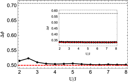
Figure 12: Phase estimation precision $\Delta\phi=1/\sqrt{F_{Q}}$, where $F_{Q}$ is the Quantum Fisher Information for the estimator $n_{L}$ in a uniform chain with $L=5$ respectively for a two particle bound state and for a three particle bound state (inset), as a function of the onsite interaction $U/J$. The red dashed/grey dotted lines represent the ideal quantum/classical lower bound, respectively $\Delta\phi_{\mathrm{quant}}=1/M$ and $\Delta\phi_{\mathrm{cl}}=1/\sqrt{M}$.

The black line on the other hand represents Eq. (14). Both for two and three particle bound states we observe an improvement in the phase estimation precision compared to the classical case, which is quite close to the ideal limit for an ideal NOON state and increases with the onsite interaction $U/J$.

VI Conclusion

In this paper we analyze the possibility to transfer states of bound particles between the endpoints of finite lattice and their use for small cat state (NOON state) generation, using a minimal control setup.

We derive an effective single particle theory for the dynamics of a bound particle state in a Bose-Hubbard model with tunable couplings, using an accurate effective Hamiltonian technique. By introducing suitable static local impurities in the edges of the lattice potential we show how to inhibit edge-localization effects and enable the bound state dynamics. This allows us to realize transformations between far sites, even when strongly interacting particles are involved. Specifically we show how state transfer coupling schemes (in particular minimal engineering schemes), developed for single particle states, can be introduced in our model to improve the efficiency. We then show how to split the propagating bound state wave-function to generate cat states (NOON states) between the endpoints of finite lattices with high fidelity, in a minimal control setup, by tuning a single local field in the middle of the chain. We analyze also how environmental effects affect our scheme, namely taking into account decoherence due spontaneous emission in an optical lattice setup, finding the parameters’ regime in which our scheme is robust.

Our model is of interest for state transfer application with $N\geq 2$ strongly interacting particles and for metrology application. In particular, compared to other systems, it can provide some advantages for sensing external local fields in a Mach-Zehnder configuration. Indeed we specifically show that, even in a uniform chain, the obtained NOON states give an improvement for the phase estimation between the output arms of an interferometer. Moreover, our method can be straightforwardly extended to fully engineered chains to realize 100% fidelity operations between distant sites, such as the perfect state transfer of bound particle states or the perfect NOON state generation in an arbitrary long chain. As a future perspective, it will be interesting to adapt pumping techniques angelakis or tunneling modulation techniques watanabe_efficient_2010 to speed up the transfer time, and thus enable the creation of higher NOON states compatible with the coherence time of the system.

Appendix A Effective Hamiltonian

For the sake of clarity and self-consistency, here we describe the effective Hamiltonian theory which has been derived and successfully applied in jia_integrated_2015 .

We assume that the Hilbert space is divided into a two subspace, the effective subspace and the irrelevant one, which are well separated in energy when the interaction strength $U$ is much greater than the chemical potential and the tunneling rates. We define a projection operator $\mathbb{P}$ which projects the states to the relevant subspace and the complementary operator $\mathbb{Q}{=}\mathbf{1}-\mathbb{P}$. Because $\mathbb{P}$ and $\mathbb{Q}$ operate onto disconnected subspaces we have

$$\mathbb{P}+\mathbb{Q} = \mathbf{1}~{},$$

$$\mathbb{P}\mathbb{Q} = \mathbb{Q}\mathbb{P}=0~{},$$ (15)

$$\mathbb{P}^{2} = \mathbb{P}~{},$$

$$\mathbb{Q}^{2} = \mathbb{Q}~{}.$$

Once Eq. (A) are applied on the Schrödinger equation, one obtains a system of two coupled equations for the dynamics in the relevant/irrelevant subspace:

$$i\partial_{t}\mathbb{P}|{\psi}\rangle = \left(\mathbb{P}H\mathbb{P}+\mathbb{P}H\mathbb{Q}\right)|{\psi}\rangle~{},$$ (16)

$$i\partial_{t}\mathbb{Q}|{\psi}\rangle = \left(\mathbb{Q}H\mathbb{P}+\mathbb{Q}H\mathbb{Q}\right)|{\psi}\rangle~{}.$$ (17)

Finally, using $\mathbb{P}^{2}{=}\mathbb{P}$ and $\mathbb{Q}^{2}{=}\mathbb{Q}$ one obtains the system

$$i\partial_{t}\left(\begin{array}[]{c}|{\psi_{p}}\rangle\\ |{\psi_{q}}\rangle\end{array}\right)=\left(\begin{array}[]{cc}H_{p}&V\\ V^{\dagger}&H_{q}\end{array}\right)\left(\begin{array}[]{c}|{\psi_{p}}\rangle\\ |{\psi_{q}}\rangle\end{array}\right)$$ (18)

whence

$$H_{p} = \mathbb{P}H\mathbb{P}~{},$$ (19)

$$H_{q} = \mathbb{Q}H\mathbb{Q}~{},$$ (20)

$$V = \mathbb{P}H\mathbb{Q}~{},$$ (21)

$$|{\psi_{P}}\rangle = \mathbb{P}\ |{\psi}\rangle~{},$$ (22)

$$|{\psi_{Q}}\rangle = \mathbb{Q}\ |{\psi}\rangle~{}.$$ (23)

Here $|{\psi_{p}}\rangle$ and $|{\psi_{q}}\rangle$ are respectively the projection of the state $|{\psi}\rangle$ in the relevant/irrelevant subspaces. In the interaction picture

$$|{\psi_{p}}\rangle = e^{-iH_{p}t}|{\hat{\phi}_{p}}\rangle~{},$$ (24)

$$|{\psi_{q}}\rangle = e^{-iH_{q}t}|{\hat{\phi}_{q}}\rangle~{},$$ (25)

the free evolution is eliminated:

$$i\partial_{t}|{\hat{\phi}_{p}}\rangle = e^{+iH_{p}t}Ve^{-iH_{q}t}|{\hat{\phi}_{q}}\rangle\equiv\hat{V}(t)|{\hat{\phi}_{q}}\rangle~{},$$ (26)

$$i\partial_{t}|{\hat{\phi}_{q}}\rangle = e^{+iH_{q}t}V^{\dagger}e^{-iH_{p}t}|{\hat{\phi}_{p}}\rangle\equiv\hat{V}^{\dagger}(t)|{\hat{\phi}_{p}}\rangle~{},$$ (27)

We introduce $U_{p}$ and $U_{q}$ the operators that diagonalize $H_{p}$ and $H_{q}$:

$$H_{p} = U_{p}\lambda_{p}U^{\dagger}_{p}~{},$$ (28)

$$H_{q} = U_{q}\lambda_{q}U^{\dagger}_{q}~{},$$ (29)

where $\lambda_{p}{=}\textrm{diag}\left\{\lambda_{p}^{i}\right\}$ and $\lambda_{q}{=}\textrm{diag}\left\{\lambda_{q}^{i}\right\}$, and defining

$$|{\tilde{\phi}_{p}}\rangle = U_{p}^{\dagger}|{\hat{\phi}_{p}}\rangle~{},$$ (30)

$$|{\tilde{\phi}_{q}}\rangle = U_{q}^{\dagger}|{\hat{\phi}_{q}}\rangle~{},$$ (31)

we have

$$i\partial_{t}|{\tilde{\phi}_{p}}\rangle = \tilde{V}(t)|{\tilde{\phi}_{q}}\rangle~{},$$ (33)

$$i\partial_{t}|{\tilde{\phi}_{q}}\rangle = \tilde{V}^{\dagger}(t)|{\tilde{\phi}_{p}}\rangle~{},$$ (34)

and

$$\tilde{V}(t)=U_{p}^{\dagger}\hat{V}(t)U_{q}=e^{i\lambda_{p}t}\hat{V}(t)e^{-i\lambda_{q}t}~{},$$ (35)

Assuming that the population of the irrelevant space is initially zero $|{\hat{\phi}_{q}(0)}\rangle=|{0}\rangle$, the formal solution of system (18) is, in components

$$\tilde{\phi}_{q,k}(t)=-i\sum\limits_{j}\int_{0}^{t}dt^{\prime}\ V_{jk}^{*}e^{i(\lambda_{q,k}-\lambda_{p,j})t^{\prime}}\tilde{\phi}_{p,j}(t^{\prime})~{},$$ (36)

After partial integration one finds

$$\begin{split}\tilde{\phi}_{q,k}(t)&=-i\sum\limits_{j}\left\{\frac{e^{i(\lambda_{q,k}-\lambda_{p.j})t^{\prime}}}{i(\lambda_{q,k}-\lambda_{p.j})}V_{jk}^{*}\tilde{\phi}_{p,j}(t^{\prime})\right|_{0}^{t}\\ &-\left.\int_{0}^{t}dt^{\prime}\ \frac{e^{i(\lambda_{q,k}-\lambda_{p.j})t^{\prime}}}{i(\lambda_{q,k}-\lambda_{p.j})}\frac{d}{dt^{\prime}}\tilde{\phi}_{p,j}(t^{\prime})\right\}~{}.\end{split}$$ (37)

The second integral can be neglected because carrying on the partial integration procedure the next term is of the order of $(\lambda_{q,k}-\lambda_{p.j})^{-2}$. Indeed for a large spectral separation between the relevant and the irrelevant subspaces, $|\lambda_{Q}^{k}-\lambda_{P}^{j}|{\gg}1$, and when the edge term is zero one has

$$\tilde{\phi}_{q,k}(t)=-\sum\limits_{j}\tilde{W}_{kj}(t)\tilde{\phi}_{p,j}(t)~{},$$ (38)

where

$$\tilde{W}_{kj}(t){=}V_{jk}^{*}\frac{\exp\left[i\left(\lambda_{Q}^{k}-\lambda_{P}^{j}\right)t\right]}{\lambda_{Q}^{k}-\lambda_{P}^{j}}~{}.$$ (39)

Finally one find that the effective Schrödinger equation for the relevant space dynamics is:

$$i\partial_{t}|{\psi_{p}}\rangle\simeq H_{\mathrm{eff}}|{\psi_{p}}\rangle~{},$$ (40)

where

$$H_{\mathrm{eff}}=H_{p}-VW~{},$$ (41)

and $W$ satisfies

$$H_{q}W-WH_{p}=V^{\dagger}.$$ (42)

When $H_{p}$ consists of a degenerate levels with energy $E_{0}$ the above effective theory corresponds to the usual degenerate perturbation theory mila_strong-coupling_2011 :

$$\langle\phi|H_{\mathrm{eff}}|\phi^{\prime}\rangle\simeq\langle\phi|H|\phi^{\prime}\rangle+\sum\limits_{m\in\mathcal{H}_{q}}\frac{\langle\phi|V|m\rangle\langle m|V|\phi^{\prime}\rangle}{E_{0}-E_{m}}+\cdots~{}.$$ (43)

where $\mathcal{H}_{p}$ and $\mathcal{H}_{q}$ are the relevant/irrelevant Hilbert subspaces and $|{\phi}\rangle,|{\phi^{\prime}}\rangle\in\mathcal{H}_{p}$.

We derive explicitly the effective Hamiltonian for a Bose-Hubbard model, Eq. (1). The Hilbert space $\mathcal{H}$ with fixed number of particle $M$ in a chain with length $L$ has size

$$\text{dim}\mathcal{H}=\frac{(M+L-1)!}{M!(L-1)!}$$ (44)

The relevant space $\mathcal{H}_{p}\equiv\mathcal{H}_{M}$ is defined as

$$\mathcal{H}_{p}=\left\{|{\psi_{m}^{b}}\rangle\in\mathcal{H}:\ |{\psi_{m}^{b}}\rangle=|{0,\ldots,0,M_{m},0,\ldots,0}\rangle\right\},$$ (45)

where $M_{m}=M$. Clearly $\text{dim}\mathcal{H}_{p}=L$. The irrelevant space $\mathcal{H}_{q}=\mathcal{H}\setminus\mathcal{H}_{p}$ is

$$\begin{split}\mathcal{H}_{q}=\left\{|{\psi_{m}^{u}}\rangle\in\mathcal{H}:\ |{\psi_{m}^{u}}\rangle=|{n_{1},\ldots,n_{L}}\rangle,\right.\\ \left.\text{where }\sum_{j}n_{j}=M\text{ and }n_{j}\neq M\right\}.\end{split}$$ (46)

Given the above definitions we rename the basis of the Hilbert space as $|{m}\rangle$, $m=1,\dots,{\rm dim}\mathcal{H}$ such that $|{m}\rangle=|{\psi^{b}_{m}}\rangle$ for $m=1,\dots,L$. The Hamiltonian then takes the following block form

$$H=\left(\begin{array}[]{c|c}H_{p}&V\\ \hline\cr V^{\dagger}&H_{q}\end{array}\right),$$ (47)

where each block can be evaluated explicitly with the following projection operators

$$\mathbb{P} =\sum_{m=1}^{L}|m\rangle\langle\psi_{m}^{b}|,$$ (48)

$$\mathbb{Q} =\sum_{m=1}^{\text{dim}H_{q}}|L+m\rangle\langle\psi_{m}^{u}|.$$ (49)

Clearly $\text{dim}\mathcal{H}_{p}=(L,L),\ \text{dim}\mathcal{H}_{q}=(\text{dim}\mathcal{H}-L,\text{dim}\mathcal{H}-L)$ and $\text{dim}V=(L,\text{dim}\mathcal{H}-L)$.

The effective Hamiltonian (41) can be computed explicitly using a series expansion for large $U_{j}=U$. The relevant Hamiltonian for the Bose-Hubbard model (1) takes the simple form

$$H_{p}=\sum_{m=1}^{L}\frac{U}{2}M(M-1)|m\rangle\langle m|-\sum_{m=1}^{L}\mu_{m}M|m\rangle\langle m|.$$ (50)

Similarly $H_{q}$ and $V$ can be computed explicitly. The effective model can be obtained by solving Eq. (41) and (42). In order to find the $W$ matrix we vectorize (see Appendix C) the Eq. (42) as

$$G\text{vec}(W)=\text{vec}(V^{\dagger}),$$ (51)

where

$$G=\left(\mathbf{1}_{\text{dim}H_{p}}\otimes H_{q}\right)-\left(H_{p}^{t}\otimes\mathbf{1}_{\text{dim}H_{q}}\right).$$ (52)

It it is convenient to write $G=G^{\text{large}}+G^{\text{small}}$ where

$$G^{\text{large}} =\mathbf{1}_{\text{dim}H_{p}}\otimes H_{q}^{\text{large}}-\left(H_{p}^{\text{large}}\right)^{t}\otimes\mathbf{1}_{\text{dim}H_{q}},$$ (53)

$$G^{\text{small}} =\mathbf{1}_{\text{dim}H_{p}}\otimes H_{q}^{\text{small}}-\left(H_{p}^{\text{small}}\right)^{t}\otimes\mathbf{1}_{\text{dim}H_{p}}.$$ (54)

and $H^{\text{large}}$ is the part of the Hamiltonian (1) that contains the terms in $U$: $H^{\text{large}}=\sum_{j=1}^{L}\frac{U}{2}n_{j}(n_{j}-1)\text{ and }H^{\text{small}}=H-H^{\text{large}}$. The system (51) can be formally solved by taking the inverse of the $G$ matrix as

$$\text{vec}(W)=\frac{1}{G^{\text{large}}+G^{\text{small}}}\text{vec}(V^{\dagger})$$ (55)

and using the following identity, valid for two operators $A$ and $B$:

$$\frac{1}{A+B}=\frac{1}{A}\left(1-B\frac{1}{A+B}\right).$$ (56)

Indeed one can easily find that

$$\begin{split}&\frac{1}{A}\left(1-B\frac{1}{A+B}\right)=A^{-1}(1-B(A+B)^{-1})=\\ &=A^{-1}\left[(A+B)(A+B)^{-1}-B(A+B)^{-1}\right]=\\ &=A^{-1}\left[A(A+B)^{-1}\right]=\frac{1}{A+B}.\end{split}$$ (57)

Using recursively the Eq. (56) one finds the Dyson expansion

$$\frac{1}{G^{\text{large}}+G^{\text{small}}}=\left(G^{\text{large}}\right)^{-1}\sum_{n=0}^{+\infty}(-1)^{n}(G^{\text{small}}\left(G^{\text{large}}\right)^{-1})^{n},$$ (58)

that corresponds to a serie expansion in the onsite interaction parameter $U$ (which is contained in $G^{\text{large}}$). Moreover,

$$G^{\text{large}}=-\frac{U}{2}\sum_{m=1}^{L}\sum_{n=1}^{\text{dim}H_{q}}g(n,m)~{}|{L{+}n,m}\rangle\langle{L{+}n,m}|,$$ (59)

where

$$g(n,m)=\sum_{j}M(M-1)\delta_{jm}-n_{j}(n_{j}-1)>0,$$

since in $\mathcal{H}_{q}$ it is $n_{j}<M$ and $\sum_{j}n_{j}=M$. Therefore, $G^{\text{large}}$ is diagonal and non-singular for each value of $M$. By truncating the expansion (58) at the relevant order $n$ in $U$ one obtains the matrix $W$ from Eq. (55) and then the effective Hamiltonian from Eq. (41), valid to the $n$-th order.

As an example of the general procedure outlined above we consider explicitly the first order solution where $M=2$ and (58) reduces to

$$(G^{\text{large}}+G^{\text{small}})^{-1} \approx(G^{\text{large}})^{-1}$$ (60)

$$=-U^{-1}\sum_{m=1}^{L}\sum_{n=1}^{\text{dim}H_{q}}|{L{+}n,m}\rangle\langle{L{+}n,m}|$$ (61)

$$=-\frac{\openone_{q}\otimes\openone_{p}}{U}~{}.$$ (62)

Therefore, according to (51), $W=-V^{\dagger}/U$, so

$$H_{\rm eff} \simeq-\sum_{m=1}^{L}\mu_{m}M|{m}\rangle\langle{m}|+\sum_{m,m^{\prime}=1}^{L}|{m}\rangle\frac{\langle{\psi_{m}^{b}}|V\mathbb{Q}V^{\dagger}|{\psi_{m^{\prime}}^{b}}\rangle}{U}\langle{m^{\prime}}|,$$ (63)

where we have explicitly omitted the terms proportional to the identity. For the interaction term $V$ between $\mathcal{H}_{p}$ and $\mathcal{H}_{q}$ we observe that the only non-zero matrix elements are $\langle\psi_{m}^{b}|a_{j}a_{j+1}^{\dagger}|\psi_{n}^{u}\rangle$ (as well as their Hermitian conjugate) when

$$|{\psi_{m}^{b}}\rangle =|{0,\ldots,M_{j},\ldots,0}\rangle$$ (64)

$$|{\psi_{n}^{u}}\rangle =|{0,\ldots,1_{j},(M-1)_{j+1},\ldots,0}\rangle.$$ (65)

These can give rise to a hopping from $|{m}\rangle$ to $|{m+1}\rangle$ only for $M=2$. Indeed, this is done with the following steps. Starting from $|{m}\rangle=|{0,\dots,2_{m},0\dots}\rangle$ the operator $a_{m}a_{m+1}^{\dagger}$ in $V$ maps this state to $|{0,\dots,1_{m},1_{m+1},0\dots}\rangle$ which is in $\mathcal{H}_{q}$. Then the operator $a_{m}a_{m+1}^{\dagger}$ in $V^{\dagger}$ maps that state to $|{m+1}\rangle=|{0,\dots,2_{m+1},0\dots}\rangle$. By generalizing the above argument, with simple calculations one finds then

$$H^{M=2}_{\rm eff} \simeq-\sum_{m=1}^{L}\mu_{m}M|{m}\rangle\langle{m}|+\sum_{m}^{L-1}\frac{J_{m}^{2}}{2U}\left(|{m}\rangle\langle{m+1}|+{\rm h.c.}\right).$$ (66)

The generalization to higher values of $M$ proceeds along the same lines. For instance for $M=3$ one has to consider the second order expansion in (58) which depends also on $G^{\text{small}}$. Indeed, an effective hopping can happen only via a three step procedure

$$|{m}\rangle =|{0,\dots,3_{m},0\dots}\rangle\to|{0,\dots,2_{m},1_{m+1}0\dots}\rangle$$ (67)

$$\to|{0,\dots,1_{m},2_{m+1}0\dots}\rangle$$ (68)

$$\to|{0,\dots,3_{m+1}0\dots}\rangle\equiv|{m+1}\rangle.$$ (69)

By doing explicit calculations we find the effective Hamiltonians mentioned in the main text.

Appendix B Minimal engineering of the Three Particle Bound state propagation

The state transfer fidelity of the three particle bound state can be improved by introducing an optimal coupling scheme, namely tuning the first and the last tunneling coupling to $J_{1}=J_{L-1}=J_{0}$ and the rest of the chain to $J_{j}=J$. We find that, in order to delocalize the bound state, two pairs of localized fields in the endpoints are necessary, respectively $\mu_{j}=-\beta_{1}(\delta_{j,1}+\delta_{j,L})$ and $\mu_{j}=-\beta_{2}(\delta_{j,2}+\delta_{j,L-1})$ where $\beta_{1}=(2J^{2}-J_{0}^{2})/8U$ and $\beta_{2}=(J^{2}-J_{0}^{2})/8U$. In this case the beam splitting condition for $L\gg 1$ is realized when a local field $\mu_{j}=-\beta\delta_{j,L/2+1}$ with strength $\beta=\tilde{\beta}J^{3}/8U^{2}$ is added in the middle of the chain. The effective Hamiltonian is it in this case

$$H_{\mathrm{opt}}^{III}/2J_{\mathrm{eff}}^{III}=\left(\begin{array}[]{ccccccc}U_{\mathrm{opt}}^{III}&\frac{J_{0}^{3}}{2J^{3}}&&&&&\\ \frac{J_{0}^{3}}{2J^{3}}&\ddots&1/2&&&&\\ &1/2&U_{\mathrm{opt}}^{III}&\ddots&&&\\ &&\ddots&U_{\mathrm{opt}}^{III}+\tilde{\beta}&\ddots&&\\ &&&\ddots&U_{\mathrm{opt}}^{III}&1/2&\\ &&&&1/2&\ddots&\frac{J_{0}^{3}}{2J^{3}}\\ &&&&&\frac{J_{0}^{3}}{2J^{3}}&U_{\mathrm{opt}}^{III}\end{array}\right)$$ (70)

where $J_{\mathrm{eff}}^{III}=3J^{3}/16U^{2}$, $U_{\mathrm{opt}}^{III}=8(U/J)^{3}+2U/J+16(J/U)^{2}$. In order to have a perfectly balanced beam splitter in this single-particle Hamiltonian, as shown in compagno_toolbox_2015 , one needs $\tilde{\beta}=1$. Therefore, $\beta^{50/50}{=}J^{3}/8U^{2}$. Our method is straightforwardly generalizable to bound states with a higher number of particles.

Appendix C Numerical solution of the master equation

In order to solve the Master equation (8) we exploit a vectorization procedure am-shallem_three_2015 which consists of representing a matrix as a vector, by using its representation in the canonical basis with a column ordering. For instance for a generic $2$x$2$ matrix $A$, its vectorization $\mathrm{vec}(A)$ is

$$A=\left(\begin{array}[]{cc}A_{11}&A_{12}\\ A_{21}&A_{22}\end{array}\right)=A_{11}\left(\begin{array}[]{cc}1&0\\ 0&0\end{array}\right)+A_{21}\left(\begin{array}[]{cc}0&0\\ 1&0\end{array}\right)+\ldots$$ (71)

$$\mathrm{vec}(A)=\left(\begin{array}[]{cccc}A_{11},&A_{21},&A_{12},&A_{22}\end{array}\right)^{t}~{}.$$ (72)

For a general size matrix $\rho$ the latter procedure corresponds to the mapping $v_{(k-1)L+j}=\rho_{jk}$ where $v=\mathrm{vec}(\rho)$. Once chosen this base the action of an operator $H$ on the left or the right of the density matrix $\rho$ can be written as

$$H\rho = \left(\mathbf{1}_{L}\otimes H\right)\mathrm{vec}(\rho)~{},$$ (73)

$$\rho H = \left(H^{t}\otimes\mathbf{1}_{L}\right)\mathrm{vec}(\rho)~{},$$ (74)

and for the dissipative part, by using the identities

$$\mathrm{vec}(ABC) = \left(C^{t}\otimes A\right)\mathrm{vec}(B)=\left(\mathbf{1}_{L}\otimes AB\right)\mathrm{vec}(C)=$$

$$= \left(C^{t}B^{t}\otimes\mathbf{1}_{L}\right)\mathrm{vec}(A)~{},$$

$$\mathrm{vec}(AB) = \left(\mathbf{1}_{L}\otimes A\right)\mathrm{vec}(B)=\left(B^{t}\otimes\mathbf{1}_{L}\right)\mathrm{vec}(A)~{},$$ (76)

we find that

$$n_{i}n_{i}\rho = \left(\mathbf{1}_{L}\otimes n_{i}n_{i}\right)\mathrm{vec}(\rho)~{},$$ (77)

$$\rho n_{i}n_{i} = \left((n_{i}n_{i})^{t}\otimes\mathbf{1}_{L}\right)\mathrm{vec}(\rho)~{},$$ (78)

$$n_{i}\rho n_{i} = \left((n_{i})^{t}\otimes n_{i}\right)\mathrm{vec}(\rho)~{},$$ (79)

hence if $H$ and $\rho$ describe a fixed particle number subspace one obtains the vectorised version of the master equation (8) namely

$$\mathrm{vec}(\dot{\rho})=\mathcal{L}_{v}\mathrm{vec}(\rho)~{},$$ (80)

where the operator $\mathcal{L}_{v}$ is defined as

$$\mathcal{L}_{v}= -i\left\{\left(\mathbf{1}_{L}\otimes H\right)-\left(H^{t}\otimes\mathbf{1}_{L}\right)\right\}-\gamma\sum\limits_{j}\left\{\left(n_{j}^{t}\otimes n_{j}\right)+\right.$$

$$-\left.\frac{1}{2}\left(\mathbf{1}_{L}\otimes n_{j}^{2}\right)-\frac{1}{2}\left((n_{j}^{2})^{t}\otimes\mathbf{1}_{L}\right)\right\}.$$

References

References

- (1) C. Weitenberg, M. Endres, J. F. Sherson, M. Cheneau, P. Schauß, T. Fukuhara, I. Bloch and S. Kuhr, Nature 471, 319 (2011).
- (2) P. M. Preiss, R. Ma, E. Tai, A. Lukin, M. Rispoli, P. Zupancic, Y. Lahini, R. Islam and M. Greiner, Science 347, 1229 (2015).
- (3) T. Fukuhara, P. Shauß, M. Endres, S. Hild, M. Cheneau, I. Bloch and C. Gross, Nature 502, 76 (2013).
- (4) T. Fukuhara, et al, Nat. Phys. 9, 235 (2013).
- (5) S. Murmann, A. Bergschneider, V. M. Klinkhamer, G. Zürn, T. Lompe and S. Jochim, Phys. Rev. Lett. 114, 080402 (2015).
- (6) P. M. Preiss, R. Ma, M. E. Tai, J. Simon and M. Greiner, Phys. Rev. A 91, 041602 (2015).
- (7) C. Robens, S. Brakhane, D. Meschede and A. Alberti, arXiv:1511.03569.
- (8) A. Celi, P. Massignan, J. Ruseckas, N. Goldman, I. B. Spielman, G. Juzeliūnas and M. Lewenstein, Phys. Rev. Lett. 112, 043001 (2014).
- (9) M. Mancini, et al, Science 349, 1510 (2015).
- (10) G. De Chiara and A. Sanpera, J. Low Temp. Phys. 165, 292 (2011).
- (11) R. Islam, R. Ma, P. M. Preiss, T. E. Tai, A. Lukin, M. Rispoli and M. Greiner, Nature 528, 77 (2015).
- (12) P. Zupancic, P. M. Preiss, R. Ma, A. Lukin, M. E. Tai, M. Rispoli, R. Islam and M. Greiner, Opt. Expr. 24, 13881 (2016).
- (13) H. Ott, Rep. Prog. Phys. 79, 054401 (2016).
- (14) D. K. Hoffmann, B. Deissler, W. Limmer and J. H. Denschlag, Appl. Phys. B 122, 227 (2016).
- (15) T. Kovachy, P. Asenbaum, C. Overstreet, C. A. Donnelly, S. M. Dickerson, A. Sugarbaker, J. M. Hogan and M. A. Kasevich, Nature 528, 530 (2015).
- (16) E. Rocco, R. N. Palmer, T. Valenzuela, V. Boyer, A. Freise and K. Bongs, New. J. Phys. 16, 093046 (2014).
- (17) H. Lee, P. Kok and J. P. Dowling, J. Mod. Opt. 49, 2325 (2002).
- (18) C. Gross, T. Zibold, E. Nicklas, J. Estève and M. K. Oberthaler, Nature 464, 1165 (2010).
- (19) C. Gross, J. Phys. B: At. Mol. Opt. Phys. 45, 103001 (2012).
- (20) J. P .Dowling, Contemp. Phys. 49, 125 (2008).
- (21) R. Demkowicz-Dobrzański, M. Jarzyna and J. Kołodyński, in Progress in Optics, Vol. 60, edited by E. Wolf (Elsevier, 2015).
- (22) Y. Israel, S. Rosen and Y. Silberberg, Phys. Rev. Lett. 112, 103604 (2014).
- (23) H. F. Hofmann and T. Ono, Phys. Rev. A 76, 031806 (2007).
- (24) I. Afek, O. Ambar and Y. Silberberg, Science 328, 879 (2010).
- (25) Y. Israel, I. Afek, S. Rosen, O. Ambar and Y. Silberberg, Phys. Rev. A 85, 022115 (2012).
- (26) P. Kok, H. Lee and J. P. Dowling, Phys. Rev. A 65, 052104 (2002).
- (27) W. J. Mullin and F. Laloë, J. Low Temp. Phys. 162, 250 (2010).
- (28) K. Stiebler, B. Gertjerenken, N. Teichmann and C. Weiss, J. Phys. B: At. Mol. Opt. Phys. 44, 055310 (2011).
- (29) G. Kordas, S. Wimberger and D. Witthaut, EPL 100, 30007 (2012).
- (30) A. M. Leung, K. W. Mahmud and W. P. Reinhardt, Mol. Phys. 110, 801 (2012).
- (31) L. Dell’Anna, G. Mazzarella, V. Penna and L. Salasnich, Phys. Rev. A 87, 053620 (2013).
- (32) K. Winkler, G. Thalhammer, F. Lang, R. Grimm, J. Hecker Denschlag, A. J. Daley, A. Kantian, H. P. Büchler and P. Zoller, Nature 76, 033606 (2007).
- (33) S. Fölling, S. Trotzky, P. Cheinet, M. Feld, R. Saers, A. Widera, T. Müller and I. Bloch, Nature 448, 1029 (2007).
- (34) D. Petrosyan, B. Schmidt, J. R. Anglin and M. Fleischhauer, Phys. Rev. A 76, 033606 (2007).
- (35) M. Valiente and D. Petrosyan, J. Phys. B: At. Mol. Opt. Phys. 41, 161002 (2008).
- (36) M. Valiente, D. Petrosyan and A. Saenz, Phys. Rev. A 81, 011601 (2010).
- (37) E. Compagno, L. Banchi and S. Bose, Phys. Rev. A 92, 022701 (2015).
- (38) L. Banchi, E. Compagno and S. Bose, Phys. Rev. A 91, 052323 (2015).
- (39) R. A. Pinto, M. Haque and S. Flach, Phys. Rev. A 79, 052118 (2009).
- (40) M. Haque, Phys. Rev. A 82, 012108 (2010).
- (41) M. Bello, C. E. Creffield and G. Platero, Sci. Rep. 6, 22562 (2016).
- (42) M. Bello, C. E. Creffield and G. Platero, arXiv:1608.00162.
- (43) A. R. Kolovsky, J. Link and S. Winberger, New. J. Phys. 14, 075002 (2012).
- (44) D. N. Maksimov, A. R. Kolovsky, Phys. Rev. A 89, 063612 (2014).
- (45) N. Jia, L. Banchi, A. Bayat, G. Dong and S. Bose, Sci. Rep. 5, 13665 (2015).
- (46) V. Alba, K. Saha and M. Haque, J. Stat. Mech., 10, P10018 (2013).
- (47) M. Lewenstein, A. Sanpera and V. Ahufinger, Ultracold Atoms in Optical Lattices (Oxford University Press, Oxford , 2012), p 51.
- (48) Y. Lahini, M. Verbin, S. D. Huber, Y. Bromberg, R. Pugatch and Y. Silberberg, Phys. Rev. A 86, 011603 (2012).
- (49) X. Qin, Y. Ke, X. Guan, Z. Li, N. Andrei and C. Lee, Phys. Rev. A 90, 062301 (2014).
- (50) A. G. Volosniev, D. Petrosyan, M. Valiente, D. V. Fedorov, A. S. Jensen and N. T. Zinner, Phys. Rev. A 91, 023620 (2015).
- (51) S. Lorenzo, T. J. G. Apollaro, S. Paganelli, G. M. Palma and F. Plastina, Phys. Rev. A 91, 042321 (2015).
- (52) T. J. G. Apollaro, S. Lorenzo, A. Sindona, S. Paganelli, G. L. Giorgi and F. Plastina, Phys. Scr., 014036 (2015).
- (53) R. Sousa and Y. Omar, New J. Phys. 16, 123003 (2014).
- (54) S. Paganelli, S. Lorenzo, T. J. G. Apollaro, F. Plastina and G. L. Giorgi, Phys. Rev. A 87, 062309 (2013).
- (55) M. Christandl, N. Datta, A. Ekert and A. J. Landahl, Phys. Rev. Lett. 92, 187902 (2004).
- (56) V. Kostak, G. M. Nikolopoulos and I. Jex, Phys. Rev. A 75, 042319 (2007).
- (57) A. Kay, J. Quant. Inf. 08, 641 (2010).
- (58) V. X. Genest, L. Vinet and A. Zhedanov, Ann. Phys. 371, 348 (2016).
- (59) J. M. Lemay, L. Vinet and A. Zhedanov, J. Phys. A 49, 335302 (2016).
- (60) L. Banchi and R. Vaia, J. of Math. Phys. 54, 043501 (2013).
- (61) L. Banchi, T. J. G. Apollaro, A. Cuccoli, R. Vaia and P. Verrucchi, New J. Phys. 13, 123006 (2011).
- (62) T. J. G. Apollaro, L. Banchi, A. Cuccoli, R. Vaia and P. Verrucchi, Phys. Rev. A 85, 052319 (2012).
- (63) A. Zwick, G. A. Álvarez, J. Stolze and O. Osenda, Phys. Rev. A 84, 022311 (2011).
- (64) A. K. Pavlis, G. M. Nikolopoulos and P. Lambropoulos, Quant. Inf. Proc., 15, 2553 (2016).
- (65) G. Kordas, D. Witthaut and S. Wimberger, Ann. der Physik 527, 619 (2015).
- (66) H. Pichler, A. J. Daley and P. Zoller, Phys. Rev. A 82, 063605 (2010).
- (67) S. Sarkar, S. Langer, J. Schachenmayer and A. J. Daley, Phys. Rev. A 90, 023618 (2014).
- (68) F. Laloë and W. J. Mullin, Found. Phys. 42, 53 (2011).
- (69) P. Hauke, M. Heyl, L. Tagliacozzo and P. Zoller, Nat. Phys., Advance Online Publication, 1 (2016).
- (70) G. Mazzarella, L. Salasnich, A. Parola and F. Toigo, Phys. Rev. A, 83, 053607 (2011).
- (71) F. Mila and K. P. Schmidt, in Introduction to Frustrated Magnetism: Materials, Experiments, Theory, Chapter 20, Springer Series in Solid-State Sciences, Vol 164, eds. C. Lacroix, F. Mila, and P. Mendels (Springer, Berlin Heidelberg, 2011) pp 537-559.
- (72) M. Am-Shallem, A. Levy, I. Schaefer and R. Kosloff, arXiv:1510.08634.
- (73) J. Tangpanitanon, V. M. Bastidas, S. Al-Assam, P. Roushan, D. Jaksch and D. G. Angelakis, arXiv:1607.04050.
- (74) G. Watanabe, Phys. Rev. A 81, 021604 (2010).