Instability in interacting dark sector: An appropriate Holographic Ricci dark energy model

Abstract

In this paper we investigate the consequences of phantom crossing considering the perturbative dynamics in models with interaction in their dark sector. By mean of a general study of gauge-invariant variables in comoving gauge, we relate the sources of instabilities in the structure formation process with the phantom crossing. In order to illustrate these relations and its consequences in more detail, we consider a specific case of an holographic dark energy interacting with dark matter. We find that in spite of the model is in excellent agreement with observational data at background level, however it is plagued of instabilities in its perturbative dynamics. We reconstruct the model in order to avoid these undesirable instabilities, and we show that this implies a modification of the concordance model at background. Also we find drastic changes on the parameters space in our model when instabilities are avoided.

I Introduction

It is well known that the measurements of the luminosity redshift of supernovae (type Ia) have proportioned growing evidence for a phase of accelerated expansion of current universeC1 ; C2 . However, other evidences of this accelerated expansion come from baryon acoustic oscillations C3 , anisotropies of the cosmic microwave background (CMB)C4 , and among other C5 , have confirmed this scenario. In order to obtain a phase of accelerated expansion in Einstein’s General Relativity it is necessary that the cosmological background dynamics be dominated by some exotic component with a negative pressure, known as dark energy (DE). Assuming that DE contributes to an important fraction of the content of the observable universe, it is instinctive and natural from the field theory to assume its interactions with other fields, e.g., dark matter (DM). It is well known that a suitable interaction between DE and DM can provide an novel mechanism to alleviate the cosmic coincidence problem C6 ; C7 . On the other hand, these models affect the structure formation and hence provide a different way to change the predictions of non-interacting models. Regarding this point, the interaction between DE and DM have been studied considering different types of observational data sets, see Refs.C8 ; C9 . For more comprehensive references of models with interacting DE and DM, see Refs.I1 ; I2 .

The study of structure formation in models of DE and DM, through the cosmological perturbations theory, plays a fundamental role when these models are confronted with the observations AC1 . These models imprint a signature on the CMB power spectrum AC2 ; AC3 and also the space of parameters is modifiedAC3 ; AC4 . For this reason the analysis of the cosmological perturbations is important and also need to be well-behaved. In particular for interacting models, the background dynamics with adiabatic initial conditions and the perturbation theory were analyzed in Ref.C10 . Here, the perturbative dynamics realizes unstable growing modes. A further analysis in models with an interacting DE component together with a constant equation of state (EoS) $w$, was considered in Ref. C11 . Here the authors found that perturbations were unstable and with a rapid growth of DE fluctuations. To avoid a possible conflict with the perturbative dynamics when the EoS parameter $w$ crosses the value $w=-1$, in Ref.Kunz:2006wc , the authors considered a new variable associated to the divergence of the velocity field. However, the new perturbations equations have a term associated to the pressure perturbation and, therefore, an adiabatic speed of sound. In this way, the authors introduced a free parameter in the adiabatic speed of sound, avoiding the divergences in the perturbations.

On the other hand, considering that observational-data tests of the $\Lambda$ cold dark matter ($\Lambda$CDM) model are not accurate enough to rule out adequately the large diversity of alternative DE models in the literature that have been proposed to account for the data. In modern cosmology, one can test the $\Lambda$CDM to describe an adequate DE model, assuming the DE as an effective fluid (or a scalar field) and considering its EoS as a free and dynamics parameter. Some candidates for this DE are the holographic models (HM) which give a specific classes of dynamic approaches to solve the cosmic coincidence problem and is another alternative to the standard $\Lambda$CDM model. These models are motivated from the Holographic principle which has its origin in the black hole and string theories HP1 . These HM have a direct connection between an ultraviolet and infrared cutoff HM1 ; HMM1 ; HMM2 . In this context, the infrared cutoff corresponds to a cosmological length scale, and by the other hand this connection between cutoffs ensures that the energy density does not exceed the energy in a given volume of a black hole of the equal size. Regarding the HM with interaction between DE and DM, this kind of models were studied in Refs.H0 ; HM2 ; HM3 . In particular we mention a specific model of HM in which the cutoff length is proportional to the Ricci scaleR1 ; V , see also Ref.V1 . In relation to the study of the dynamics of perturbations, this was analyzed in Refs.V0 ; V2 . The appearance of instabilities in the dark sector, through the perturbative dynamics, occurs when the EoS parameter $w$ crosses the value $w=-1$ in models with a dynamical EoS. In this context, the study of this crossing of the EoS parameter and the appearance of instabilities in the perturbative dynamics for non-interacting Ricci holographic model, was performed in Ref.DelCampo2013 .

In the present paper we study the background dynamics and also present the analysis of linear perturbations in the framework of gauge-invariant variables in comoving gauge, for the interacting dark sector, identifying the source of instabilities. In particular we consider that the dark energy density corresponds to the holographic Ricci DE model, and then we extended the study developed in Ref.DelCampo2013 , but now considering an interacting dark sector. Here we study the background equations, the linear perturbations and the appearance of instabilities. In order to evade these instabilities we develop an appropriate holographic Ricci interacting dark energy model and we find drastic changes on the constraints of the parameters.

This article is organized as follows. In Sect. II we present the background equations for the interacting dark sector. In Sect. III we analyze the dynamics of perturbations in a general framework for a single fluid and two interacting fluids. In Sect. IV we study the evolution of linear perturbations and identify the sources of instabilities. In Sect. V we consider a specific holographic dark energy model, known as Ricci DE. Here we study the background dynamics and analyze the observational tests on this model, considering the SNIa and $H(z)$ data sets. In Sect.VI we study the linear perturbations and identify the instabilities in our interacting model. We also analyze the high-redshift limit of our model and we compare it with $\Lambda$CDM model. In Sect. VII we study how to avoid these instabilities and develop an appropriate model . Finally, Sect. VIII summarizes our results and exhibits our conclusions.

II Background equations: dark energy- dark matter interaction

We consider a spatially flat Friedmann- Roberson-Walker universe dominated by two interacting components, dark energy (subscript $x$) and dark matter (subscript $m$) that behaves as pressureless dust. In this form, the total energy density is given by $\epsilon=\epsilon_{m}+\epsilon_{x}$ and the Friedmann equation can be written as

$$3H^{2}=\epsilon=\epsilon_{m}+\epsilon_{x},$$ (1)

where $H=\dot{a}/a$ is the Hubble rate and $a$ is the scale factor. For convenience we will use the units in which $8\pi G=c=\hbar=1$, and the dots mean derivatives with respect to the cosmological time.

On the other hand, we assume that both energy densities do not evolve separately, but rather they interact with each other through a source term, that enters the energy balance equations as

$$\dot{\epsilon}_{m}+3H\epsilon_{m}=Q,\,\,\;\;\mbox{and}\,\,\,\;\;\;\dot{\epsilon}_{x}+3H(\epsilon_{x}+p_{x})=-Q,$$ (2)

here $Q$ denotes the interaction term. If $Q>0$, the direction of energy transfer is from DE to DM, if $Q$ is negative then the direction of energy transfer occurs from DM to DE. We note that the total energy density $\epsilon=\epsilon_{m}+\epsilon_{x}$ is conserved. We also consider that the DE component obeys an EoS, such that $w_{x}\equiv\frac{p_{x}}{\epsilon_{x}}=\frac{p}{\epsilon_{x}}\equiv w$, where $w$ corresponds to the EoS parameter. Here the quantity $p_{x}$ denotes the pressure associated with the DE. In virtue of these quantities, the acceleration equation becomes

$$\dot{H} = -\frac{3}{2}H^{2}\left(1+\frac{w}{1+r}\right),\,\,\;\mbox{or equivalently}\;\,\,\,\,\,\frac{d\ln H}{d\ln a}=-\frac{3}{2}\left(1+\frac{w(a)}{1+r(a)}\right),$$ (3)

where $r\equiv\frac{\epsilon_{m}}{\epsilon_{x}}$ denotes the ratio between both energy densities. We also note that the total effective EoS of the cosmic medium $w_{total}=p/\epsilon$ can be written as

$$w_{total}=\frac{p}{\epsilon}=\frac{p_{x}}{\epsilon_{m}+\epsilon_{x}}=\frac{w}{1+r}.$$ (4)

From (2), the rate of change of the ratio between both energy densities $r$ becomes

$$\dot{r}=3Hr(1+r)\left[\frac{w}{1+r}+q_{m}\right]=3Hr(1+r)\left[w_{total}+q_{m}\right],$$ (5)

where the quantity $q_{m}$ is defined as

$$q_{m}\equiv\frac{Q}{3H\epsilon_{m}}.$$ (6)

In particular in the absence of interaction, we have that $q_{m}=0$.

III General remarks on perturbations: interacting model

III.1 Single fluid

In order to motivate the analysis of cosmological perturbations in DE models and its dynamics, we start by reviewing the perturbations for a single fluid.

We consider the dark sector has an energy-momentum tensor of a perfect fluid given by $T_{\mu\nu}=\epsilon u_{\mu}u_{\nu}+ph_{\mu\nu}$, where the tensor $h_{\mu\nu}$ is defined as $h_{\mu\nu}=g_{\mu\nu}+u_{\mu}u_{\nu}$ and $u_{\mu}\,u^{\mu}=-1$. Here, again $\epsilon$ represents the energy density, $p$ the pressure and $u^{\mu}$ corresponds to the 4-velocity of the dark fluid. From the conservation law of the energy-momentum tensor $T^{\mu\nu}_{;\nu}$=0, we obtain that the equations for timelike and spacelike parts are given by

$$\epsilon_{,\alpha}u^{\alpha}+\Theta\left(\epsilon+p\right)=0\,,$$ (7)

and

$$\left(\epsilon+p\right)\dot{u}^{\mu}+p_{,\alpha}h^{\alpha\mu}=0\,,$$ (8)

respectively. Here, the quantity $\Theta\equiv u^{\mu}_{;\mu}$ is the expansion scalar and $\dot{u}\equiv u^{\mu}_{;\nu}u^{\nu}$.

In order to calculate the perturbations, we consider the most general flat metric , containing only scalar perturbations of a homogeneous and isotropic background given by

$$\mbox{d}s^{2}=-\left(1+2\phi\right)\mbox{d}t^{2}+2a^{2}F_{,i}\mbox{d}t\mbox{d}x^{i}+a^{2}\left[\left(1-2\psi\right)\delta_{ij}\right.+\left.2E_{,i\,j}\right]\mbox{d}x^{i}\mbox{d}x^{j},\,$$ (9)

where $\phi=\phi(t,{\bf{x}})$, $F=F(t,{\bf{x}})$, $\psi=\psi(t,{\bf{x}})$ and $E=E(t,{\bf{x}})$ are metric perturbation, see Ref.bardee .

For the 4-velocity $u_{\mu}=(u_{0},u_{i})$ we get

$$u_{0}=1-\phi,\;\;\;\;\;\mbox{and}\qquad\,u_{i}=v_{,i}\,,$$ (10)

where $v$ denotes the scalar velocity perturbation. Considering the metric (9), we find that the quantity $\Theta=3H$, and its perturbation $\delta\Theta$ is given by

$$\delta\Theta=\frac{\nabla^{2}}{a^{2}}\left(v+\chi\right)-3\dot{\psi}-3H\phi\,,\,\,\,\mbox{where}\qquad\chi=\left(\dot{E}-F\right)\,.$$ (11)

The Eq. (7) can be rewritten up to zeroth and also to first order of perturbations, yielding

$$\dot{\epsilon}+\Theta\left(\epsilon+p\right)=0\,,\,\,\,\mbox{and}\qquad\dot{\delta\epsilon}-\dot{\epsilon}\phi+\delta\Theta\left(\epsilon+p\right)+\Theta\left(\delta\epsilon+\delta p\right)=0\,.$$ (12)

Usually the right equation of (12) can be written in function of density contrast defined as $\delta=\frac{\delta\epsilon}{\epsilon}$. However, the quantity $\delta$ is not gauge-invariant. Thus is suitable to describe the dynamics of perturbations in terms of gauge-invariant variables. In particular, in comoving gauge, these invariant quantities represent perturbations on comoving hypersurfaces. In the following, we will denote a superscript $c$ to all gauge-invariants in comoving gauge. These invariant quantities are defined as $\delta^{c}=\delta+\frac{\dot{\epsilon}}{\epsilon}\,v$, $\delta\Theta^{c}=\delta\Theta+\dot{\Theta}v$ and $\delta p^{c}=\delta p+\dot{p}\,v$, see Ref.Hipolito2009 . In virtue of these gauge-invariant quantities the right equation of (12) can be rewritten as

$$\dot{\delta}^{c}-\Theta\frac{p}{\epsilon}\delta^{c}+\left(1+\frac{p}{\epsilon}\right)\delta\Theta^{c}=0\,,$$ (13)

or equivalently

$$\delta^{c\prime\prime}+\left[\frac{3}{2}-\frac{15}{2}\frac{p}{\epsilon}+3\frac{p^{\prime}}{\epsilon^{\prime}}\right]\frac{\delta^{c\prime}}{a}-\left[\frac{3}{2}+12\frac{p}{\epsilon}-\frac{9}{2}\frac{p^{2}}{\epsilon^{2}}-9\frac{p^{\prime}}{\epsilon^{\prime}}\right]\frac{\delta^{c}}{a^{2}}+\frac{k^{2}}{a^{2}H^{2}}\frac{\delta p^{c}}{\epsilon a^{2}}=0\,,$$ (14)

where the primes denote derivatives with respect to the scale factor $a$ (for more details, see Refs.vomMarttens2014 ; Funo2014 ). Here we point out that this equation governs the dynamics of perturbations for the dark sector as a whole. Also considering at first order Eq.(8), we find the momentum balance equation becomes

$$\dot{v}+\phi+\frac{\delta p^{c}}{\epsilon+p}=0\,.$$ (15)

III.2 Interacting Two-component fluid: General Formalism

In this subsection we consider a general formalism to study the perturbative dynamics for two interacting fluids: DM that behaves as pressureless dust and DE. In the following, we will consider that both components are interacting and then the energy momentum tensor for each individual component is not conserved separately, i.e., $T^{\mu\nu}_{A;\nu}=Q^{\mu}_{A}$. Here $Q^{\mu}_{A}$ denotes the energy-momentum transfer vector between both fluids and ”A” label denotes both components: $A=m$ for dark matter and $A=x$ for dark energy.

By considering the timelike part of the balance equation and from the projection in the direction of the vector $u_{A\mu}$, we find that

$$\epsilon_{A,\mu}u^{\mu}_{A}+\Theta_{A}\left(\epsilon_{A}+p_{A}\right)=-u_{A\mu}Q^{\mu}_{A}=Q_{A}\,.$$ (16)

In general the expansion scalar $\Theta_{A}=u^{\mu}_{A;\mu}$ is different for each component of the dark sector, however up to zero order, or equivalently at the background level, the 4-velocities are $u^{\mu}_{m}=u^{\mu}_{x}=u^{\mu}$, then $\Theta_{A}=\Theta=3H$. We emphasize that Eq.(16) corresponds to the projections of vector $Q^{\alpha}_{A}$ along the 4-velocity $u_{A\alpha}$. In this way, the scalar quantity $u_{m\alpha}Q^{\alpha}=-u_{x\alpha}Q^{\alpha}_{x}=u_{\alpha}Q^{\alpha}=Q$. On the order hand, the perturbed time components of the 4-velocities, to first order, are given by $\delta u_{0}=\delta u^{0}=\delta u^{0}_{m}=\delta u^{0}_{x}=-\phi$.

Now the energy-momentum balance equations are given by taking the spacelike part of the vector $T^{\mu\nu}_{A;\nu}=Q^{\mu}_{A}$, resulting in

$$\left(\epsilon_{A}+p_{A}\right)\dot{u}_{A\mu}+p_{A,\alpha}h^{\alpha}_{A\mu}=h_{A\mu\alpha}Q^{\alpha}_{A}={\cal{Q}}_{A\mu}\,,$$ (17)

where again $\dot{u}_{A,\beta}=u^{\alpha}_{A;\beta}u_{A\alpha}$ and $p_{A}$ denotes the pressure of the $A$-fluid. Following Refs.q1 ; q2 the energy-momentum transfer $Q^{\alpha}$, can be decomposed in two parts, one proportional and other perpendicular to the total 4-velocity $u^{\alpha}$, so that

$$Q^{\alpha}=u^{\alpha}Q+{\cal{Q}}^{\alpha},\,\,\,\mbox{such that}\qquad u_{\alpha}{\cal{Q}}^{\alpha}=0,\,\,\,\mbox{and}\qquad Q=-u_{\mu}Q^{\mu}.$$ (18)

Also, we note that this decomposition of the vector $Q^{\alpha}$ implies that at first order, ${\cal{Q}}^{\alpha}=(0,{\cal{Q}}^{i})$, where ${\cal{Q}}^{i}$ corresponds to spatial vector up to first order. In virtue of these quantities, Eq. (16) for dark matter and for dark energy may be rewritten as

$$\epsilon_{m,\alpha}u^{\alpha}+\Theta_{m}\,\epsilon_{m}=Q\,,\,\;\;\;\mbox{and}\qquad\epsilon_{x,\alpha}u^{\alpha}+\Theta_{x}\,(\epsilon_{x}+p_{x})=-Q\,,$$ (19)

respectively. For the dark matter, we find that the energy balance can be obtained considering at first order of Eq. (16) in which

$$\dot{\delta\epsilon}_{m}-\dot{\epsilon}_{m}\phi+\Theta\delta\epsilon_{m}+\epsilon_{m}\delta\Theta_{m}=-\delta\left(u_{m\alpha}Q^{\alpha}\right)=\delta Q\,,$$ (20)

whereas for the dark energy we get

$$\dot{\delta\epsilon}_{x}-\dot{\epsilon}_{x}\phi+\Theta\left(\delta\epsilon_{x}+\delta p_{x}\right)+\delta\Theta_{x}\left(\epsilon_{x}+p_{x}\right)=\delta\left(u_{x\alpha}Q^{\alpha}\right)=-\delta Q\,.$$ (21)

Here we have introduced the functions of contrast of matter density $\delta_{m}=\frac{\delta\epsilon_{m}}{\epsilon_{m}}$ and dark energy density $\delta_{x}=\frac{\delta\epsilon_{x}}{\epsilon_{x}}$ respectively. However, these densities are not gauge-invariants and we shall describe our results in terms of gauge-invariants in comoving gauge. Following Ref.Vargas2012 we will consider the invariant quantities $\delta\Theta^{c}_{m}=\delta\Theta_{m}+\dot{\Theta}v$, $\delta^{c}_{m}=\delta_{m}+\frac{\dot{\epsilon}_{m}}{\epsilon_{m}}v$, and $\delta Q^{c}=\delta Q+\dot{Q}v$ in the comoving gauge. In this way, at first order the gauge-invariant equation for the dark matter contrast can be rewritten as

$$\dot{\delta}^{c}_{m}+\frac{\dot{\epsilon}_{m}}{\epsilon_{m}}\frac{\delta p^{c}}{\epsilon+p}+\delta\Theta^{c}_{m}=\frac{\delta Q^{c}}{\epsilon_{m}}-\frac{Q}{\epsilon_{m}}\delta^{c}_{m}.$$ (22)

Considering the most general perturbed metric given by Eq.(9), we find that the scalar perturbation $\Theta_{A}$ can be written as Funo2014

$$\delta\Theta_{A}=\frac{\nabla^{2}}{a^{2}}\left(v_{A}+\chi\right)-3\dot{\psi}-3H\phi\,,\,\,\,\,\mbox{where}\qquad\chi=\left(\dot{E}-F\right).$$ (23)

Here we have considered that $\Theta_{A}=u^{\mu}_{A;\mu}$, which corresponds to the scalar expansion for the $A$-component.

Also, at first order the energy-momentum balance Eq.(17) for both dark fluids becomes

$$\epsilon_{m}\left(\dot{v}_{m}+\phi\right)_{,i}={\cal{Q}}_{i}\,,\,\,\,\mbox{and}\qquad\left(\epsilon_{x}+p_{x}\right)\left(\dot{v}_{x}+\phi\right)_{,i}+\delta p^{c_{x}}_{,i}=-{\cal{Q}}_{i},$$ (24)

respectively. Here we mention that the combination $\dot{v}+\phi$ is a gauge-invariant quantity in the comoving gauge, and the quantity $p^{c_{x}}$ is defined as $p^{c_{x}}\equiv\delta p_{x}^{c}+\dot{p}_{x}v_{x}=\delta p^{c}+\dot{p}v_{x}$ i.e., comoving to the dark energy

IV Linear perturbations and source of instabilities: Relative energy-density perturbation

In order to analyze the perturbative dynamics in terms of gauge-invariant quantities, we will study the linear perturbations considering the relative energy-density perturbation $S^{c}$. Following Ref.DelCampo2013 we introduce the relative energy-density perturbation $S^{c}$, defined as $S^{c}=\Delta^{c}-\delta^{c}_{m}$, where $\Delta^{c}=\frac{\delta\epsilon^{c}}{\epsilon+p}$. As it was noticed in Ref.DelCampo2013 , the instabilities in the perturbative dynamics of the fluids are described in terms of this function.

In order to find the equation for the variable $S^{c}$, we need to rewrite Eq.(13) in terms of the dimensionless variable $\Delta^{c}$. Considering Ref.Hipolito2009 we have that

$$\Delta^{c}-\Theta\frac{\dot{p}}{\dot{\epsilon}}\Delta^{c}+\delta\Theta^{c}=0\,,$$ (25)

and now, combining with Eq.(22), we find that the equation for the relative perturbation $S^{c}$ results

$$\dot{S}^{c}+\Theta\,\frac{\delta p^{c}_{nad}}{\epsilon+p}+\delta\Theta^{c}-\delta\Theta^{c}_{m}=G\,,$$ (26)

where the function $G$ is defined as

$$G=G(q_{m},\delta Q^{c})=-\frac{\delta Q^{c}}{\epsilon_{m}}+3Hq_{m}\delta^{c}_{m}+3Hq_{m}\frac{\delta p^{c}}{\epsilon+p}.$$

Here, $\delta p^{c}$ corresponds to the gauge-invariant expression for pressure perturbation of the dark fluid, and the quantity $\delta p^{c}_{nad}$ denotes the non-adiabatic contribution of the pressure of the dark fluid. We mention that the relation between both quantities is given by $\delta p_{nad}=\delta p^{c}-\frac{\dot{p}}{\dot{\epsilon}}\delta\epsilon^{c}$. Also, by considering the interaction to first order and the comoving gauge, the quantities $\delta Q^{c}$ and $\delta\Theta^{c}$ are defined as $\delta Q^{c}=\delta Q+\dot{Q}v$ and $\delta\Theta^{c}=\delta\Theta+\dot{\Theta}v$, respectively.

Adding Eqs.(20) and (21) and comparing with Eq.(12), we get

$$\delta\Theta^{c}=\frac{\epsilon_{m}}{\epsilon+p}\delta\Theta_{m}^{c}+\frac{\epsilon_{x}+p_{x}}{\epsilon+p}\delta\Theta_{x}^{c}\,,$$ (27)

which allow us to write

$$\delta\Theta^{c}-\delta\Theta_{m}^{c}=\left(1-\frac{\epsilon_{m}}{\epsilon+p}\right)\left(\delta\Theta_{x}^{c}-\delta\Theta_{m}^{c}\right)=\left(1-\frac{\epsilon_{m}}{\epsilon+p}\right)\frac{\nabla^{2}}{a^{2}}\left(v_{x}-v_{m}\right)\,,$$ (28)

where we have used Eq.(23). Now combining Eqs.(24), (26), and (28), we find that the equation for the relative energy-density becomes

$$S^{c\prime\prime}+\left(1+a\frac{H^{\prime}}{H}+\tilde{A}(a)\right)\frac{S^{c\prime}}{a}+\tilde{B}(a)=0,$$ (29)

where

$$\tilde{A}(a)=\frac{3r}{1+w}(q_{m}+\hat{c^{2}_{s}})+2,\,\qquad\hat{c}^{2}_{s}\equiv\frac{p^{\prime}}{\epsilon^{\prime}},$$ (30)

and

$$\tilde{B}(a)=\frac{1}{aH}\left[\frac{3H}{\epsilon+p}\delta p^{c}_{nad}\right]^{\prime}+\frac{\tilde{A}(a)}{a^{2}H}\left[\frac{3H}{\epsilon+p}\delta p^{c}_{nad}\right]-\frac{\nabla^{2}}{a^{4}H^{2}}\frac{\delta p^{c_{x}}}{\epsilon+p}$$

$$-\frac{{\cal{Q}}}{a^{2}H^{2}\epsilon_{m}}-\tilde{A}(a)\frac{G}{a^{2}H}-\frac{G^{\prime}}{aH}.$$ (31)

Here, we observe that in the limit $Q\rightarrow 0$, the function $\tilde{A}(a)$ corresponds to the obtained in Ref.DelCampo2013 . As before the primes denote derivatives with respect to the scale factor and $\hat{c}_{s}$ denotes the total adiabatic speed of sound.

In this form, Eqs.(14) and (29) are the fundamental equations that govern the dynamics of perturbations in the case of interacting DE and DM fluids, since it allows us to find the perturbations $\delta^{c}_{m}$ and $\delta^{c}_{x}$. We mention that the Eqs.(14) and (29) are coupled (as we shall see in the next sections) and the sources of this coupling are the functions $\delta p_{nad}$, $\delta p^{c}_{x}$, and the interaction term $q_{m}$.

At this point we observe that, if any DE model has a dynamic EoS and it crosses the value $w=-1$ in any finite time, then there will exist a source of instabilities driven by the function $\tilde{A}(a)$. In particular, these instabilities shall appear in matter perturbations via the $S^{c}$-function independently of whether DE and DM are interacting or not. As we will mention in the next subsection, terms related to $\delta p^{c}_{nad}$ and $G$ do not present divergences. However we will have another contribution to the instabilities arising from the term related to the pressure perturbations $\delta p^{c_{x}}$.

IV.1 Pressure terms and perturbative dynamics

An interesting feature of the equations for $\delta^{c}$ and $S^{c}$ is that they are directly related to the non-adiabatic total pressure perturbation $\delta p^{c}$ and the dark energy pressure perturbation $\delta p^{c}_{x}$. In the following, we will express these two pressure perturbations as functions of $\delta^{c}$ and $S^{c}$, and then we will analyze the instabilities and its sources. Following Ref.Hipolito2010 , the non-adiabatic part of the total pressure perturbation $\delta p_{nad}$, can be written as

$$\delta p_{nad}^{c}=\delta p_{x,nad}^{c}+\epsilon_{m}\frac{\epsilon_{x}+p_{x}}{\epsilon+p}\frac{\dot{p}_{x}}{\dot{\epsilon}_{x}}\left(\frac{\delta\epsilon_{x}^{c}}{\epsilon_{x}+p_{x}}-\delta_{m}^{c}\right),$$ (32)

where

$$\,\delta p_{x,nad}^{c}=\delta p_{x}^{c}-\frac{\dot{p}_{x}}{\dot{\epsilon}_{x}}\delta\epsilon_{x}^{c}\,.$$

Here, $\delta p^{c}_{x,nad}$ corresponds to the non-adiabatic part of the dark energy pressure perturbation, which is intrinsic to dark energy. The equation for the total pressure perturbation $\delta p_{nad}$, given by Eq.(32), can be rewritten as

$$\delta p_{nad}^{c}=\delta p_{x,nad}^{c}+c^{2}_{s}\frac{\epsilon_{m}}{\epsilon+p}\left[-q_{m}\epsilon\delta^{c}+(\epsilon+p)S^{c}\right],$$ (33)

where the sound speed becomes

$$c^{2}_{s}\equiv\frac{p^{\prime}_{x}}{\epsilon^{\prime}_{x}}=w-\frac{1}{3}\frac{r(w+q_{m}+q_{m}r)}{q_{m}r+1+w}.$$

Here, we observe that in the limit $Q\rightarrow 0$ the sound speed $c^{2}_{s}$ has a divergence in the case when the EoS parameter $w\rightarrow-1$ and the dynamic of the pressure perturbations collapse. However, in the case with interaction, we note that the sound speed is finite when $w\rightarrow-1$ and this divergence does not occur in our case.

From Eq.(33) we observe that the non-adiabaticity of the dark sector arises from the non-adiabaticity of the dark energy and the relative entropy (the second term of Eq.(32)) between dark energy and dark matter fluid and also from the interaction $q_{m}\propto Q$ (see Eq.(6)). Now, and considering for simplicity that the dark energy is an adiabatic fluid, i.e., $\delta p_{x,nad}=0$, then from Eq.(33) the contribution to the non-adiabatic total pressure perturbation arises from the relative entropy between DM-DE and the interaction term $q_{m}$. In this form, the total pressure perturbation $\delta p^{c}=\delta p_{nad}+\dot{p}/\dot{\epsilon}\,\delta\epsilon^{c}$ reduces to

$$\delta p^{c}=(\hat{c}^{2}_{s}-q_{m}y_{1})\epsilon\delta^{c}+c^{2}_{s}\epsilon\frac{r}{1+r}S^{c}\,,$$ (34)

where

$$\hat{c}^{2}_{s}=\frac{c^{2}_{s}(q_{m}r+1+w)}{1+r+w}\,,\,\,\,\,\mbox{and}\qquad y_{1}=\frac{rc^{2}_{s}}{1+r+w}.$$ (35)

From Eq.(34) the term $3H\,\frac{\delta p_{nad}^{c}}{\epsilon+p}$ can be written as

$$3H\frac{\delta p_{nad}^{c}}{\epsilon+p}=f_{1}\delta^{c}+f_{2}S^{c},$$ (36)

where

$$f_{1}\equiv-3Hq_{m}(1+r)y_{1},\,\,\,\,\,f_{2}=3Hy_{1}.$$ (37)

Under the assumption that $\delta p_{x,nad}=0$, the function $G$ given by Eq.(26) takes the form

$$G=-\frac{\delta Q^{c}}{\epsilon_{m}}+g_{1}\delta^{c}+g_{2}S^{c},$$ (38)

where the coefficients $g_{1}$ and $g_{2}$ are given by

$$g_{1}\equiv 3Hv_{1}(1+\hat{c}_{s}^{2}-q_{m}y_{1}),\,\,\,\,\,g_{2}\equiv 3Hq_{m}\left(y_{1}-1\right),\,\,\;\;\mbox{and}\,\,\,\,\;\,\,v_{1}\equiv\frac{q_{m}(1+r)}{1+r+w},$$ (39)

respectively. Here we have considered Eq.(34).

In order to find the coupled set of equations for $\delta^{c}$ and $S^{c}$, with a general interaction term $Q$ and thus $\delta Q^{c}$, we need to find an expression for the pressure perturbation associated to the dark energy component $\delta p^{c_{x}}$ such that

$$\delta p^{c_{x}}=\delta p^{c}+\dot{p}v_{x}=\delta p^{c}+\dot{p}v+\dot{p}(v_{x}-v)=\delta p+\dot{p}(v_{x}-v),$$ (40)

where the difference between the scalar velocity perturbations $v_{x}-v$ is given by

$$v_{x}-v=\frac{\epsilon_{m}}{\epsilon+p}(v_{x}-v_{m}).$$ (41)

Now, and going to the $k$-space, where $k$ denotes the magnitude of the physical momentum ($k=|{\bf{k}}|$), we find that the difference between the velocity perturbation of DE and DM, $v_{x}-v_{m}$ results

$$v_{x}-v_{m}=\frac{a^{2}}{k^{2}}\frac{\epsilon+p}{\epsilon_{x}+p_{x}}\left[S^{c\prime}aH+(f_{1}-g_{1})\delta^{c}+(f_{2}-g_{2})S^{c}+\frac{\delta Q^{c}}{\epsilon_{m}}\right].$$ (42)

Here, we have considered Eqs.(26), (28), and (38), respectively.

In this way, the quantity $\frac{\delta p^{c_{x}}}{\epsilon+p}$ appearing in Eq.(31) becomes

$$\frac{\delta p^{c_{x}}}{\epsilon+p} = -3Hy_{1}\frac{k^{2}}{a^{2}}\left(1+q_{m}\frac{r}{1+w}\right)\left[(f_{1}-g_{1})\delta^{c}+(f_{2}-g_{2})S^{c}+aHS^{c\prime}+\frac{\delta Q^{c}}{\epsilon_{m}}\right]$$ (43)

$$+v_{1}\left(\frac{\hat{c}_{s}^{2}}{q_{m}}-y_{1}\right)\delta^{c}+y_{1}S^{c}.$$

We note that the expression given by Eq.(43) which appears in the Eq.(31), is also (joint with $\tilde{A}(a)$) responsible of the instabilities in the perturbative dynamics when the dynamical EoS parameter $w$ crosses the value $w=-1$.

Considering Eq.(34), we determine the equation for the gauge-invariant quantity $\delta^{c}$ given by

$$\delta^{c\,\prime\prime}+\left[\frac{3}{2}-\frac{15}{2}\frac{w}{1+r}+3\hat{c}^{2}_{s}\right]\frac{\delta^{c\,\prime}}{a}-\left[\frac{3}{2}+\frac{12w}{1+r}-\frac{9}{2}\left(\frac{w}{1+r}\right)^{2}-9\hat{c}^{2}_{s}+\frac{k^{2}}{a^{2}H^{2}}(q_{m}y_{1}-\hat{c}^{2}_{s})\right]\frac{\delta^{c}}{a^{2}}$$

$$=-\frac{k^{2}c^{2}_{s}}{a^{2}H^{2}}\frac{r}{1+r}\frac{S^{c}}{a^{2}}\,.$$ (44)

Also from Eqs.(29), (31), (36), (38), and (43), the equation for the relative energy-density perturbation can be written

$$S^{c\,\prime\prime}+\left[1+m+\frac{y_{2}}{H}\right]\frac{S^{c\,\prime}}{a}+\left[\frac{a}{H}y_{2}^{\,\prime}+\frac{y_{2}}{H}\left(m+\frac{3}{2}+\frac{3}{2}\frac{w}{1+r}\right)+\frac{k^{2}y_{1}}{a^{2}H^{2}}\right]\frac{S^{c}}{a^{2}}+\frac{v_{2}}{H}\frac{\delta^{c\,\prime}}{a}$$

$$+\left[\frac{a}{H}v_{2}^{\,\prime}+\frac{v_{2}}{H}\left(m+\frac{3}{2}+\frac{3}{2}\frac{w}{1+r}\right)+\frac{k^{2}v_{1}}{a^{2}H^{2}}\left(\frac{\hat{c}^{2}_{s}}{q_{m}}-y_{1}\right)\right]\frac{\delta^{c}}{a^{2}}$$

$$=-\frac{1}{a^{2}H}\left(m+\frac{3}{2}+\frac{3}{2}\frac{w}{1+r}\right)\frac{\delta Q^{c}}{\epsilon_{m}}-\frac{1}{aH}\left(\frac{\delta Q^{c}}{\epsilon_{m}}\right)^{\,\prime},$$ (45)

where the function $m$ is defined as

$$m=\frac{1}{2}-\frac{3}{2}\frac{w}{1+r}+\frac{3r}{1+w}(q_{m}+\hat{c}^{2}_{s}-q_{m}y_{1})-3y_{1},$$ (46)

with

$$y_{2}=3H\left[y_{1}(1-q_{m})+q_{m}\right]\,,\,\,\,\,\mbox{and}\qquad v_{2}=3Hv_{1}\left(q_{m}y_{1}-c_{s}^{2}r-1-\hat{c}^{2}_{s}\right).$$ (47)

The general Eqs. (44) and (45) allow us to obtain the solutions for the perturbations of the dark sector, consisting in DE and DM fluids, interacting through a $Q$ term and, accordingly, its perturbation $\delta Q^{c}$. Also we note that in the limit in which $Q$ equals to zero, the Eqs. (44) and (45) reduce to the equations obtained in Ref.DelCampo2013 .

As a concrete example, in the next section we will study a particular dynamical interacting dark energy model, where the energy density of the dark energy component has a holographic nature. In this form we will extend the work performed in Ref.DelCampo2013 adding an interaction between DM and Ricci-DE fluids. Also we shall illustrate, how a well-situated model from point of view of observational background tests, could be plagued of instabilities in its perturbative dynamics.

V Ricci dark energy: background dynamics

In this section we describe a cosmological interacting dark energy model, where the DE corresponds to the holographic Ricci model.

We begin by summarizing the characteristic of holographic DE with an energy density of energy $\epsilon_{x=H}\equiv\epsilon_{H}$, which interacts with dark matter $\epsilon_{m}$. Also the energy density of each component is related to the total dark sector with energy density ($\epsilon=\epsilon_{H}+\epsilon_{m}$), through $\epsilon_{m}=r(1+r)^{-1}\epsilon$ and $\epsilon_{H}=(1+r)^{-1}\epsilon$, where, as before, the rate $r$ is defined as $r=\frac{\epsilon_{m}}{\epsilon_{H}}$.

Following Refs.HM1 ; HMM1 holographic energy density is given by

$$\epsilon_{H}=3\,c^{2}\,L^{-2},$$ (48)

where $c^{2}$ is a constant and the factor 3 was introduced for mathematical convenience. On the other hand, the quantity $L$ is an infrared cutoff scale. Different alternatives of the infrared cutoff $L$ have been studied in the literature, see e.g., Refs.HM1 ; R1 ; V .

Differentiating Eq.(48) and considering Eq.(2) we get

$$\frac{Q}{\epsilon_{H}}=2\frac{\dot{L}}{L}-3H(1+w)\,.$$ (49)

In particular for the special case in which $Q=0$, the EoS parameter becomes $w=(2\dot{L}-3HL)/3HL$ and coincides with the obtained in Ref.DelCampo2011 .

Following Refs.R1 ; V the cutoff scale is given by $L^{2}=6R^{-1}$, where $R$ corresponds to the Ricci scalar $R=6(2H^{2}+\dot{H})$ and then, the dark energy density becomes $\epsilon_{H}=3c^{2}(2H^{2}+\dot{H})$.

From Eqs.(1) and (3) the EoS parameter becomes

$$w=\frac{1+r}{3}-\frac{2}{3c^{2}},\,\,\,\,\,\mbox{then}\qquad 3\dot{w}=\dot{r},\,\,\;\;\mbox{and}\qquad r=r_{0}+3(w-w_{0})\,,$$ (50)

here we observe that the parameter $c^{2}$ is associated to $r_{0}$ and $w_{0}$, such that $c^{2}=2(r_{0}-3w_{0}+1)^{-1}$.

Deriving the Ricci DE, for which $\epsilon_{H}\propto R$, and combining with Eq.(2), we find a relation between the EoS parameter $w$ and the interaction term $Q$, given by

$$\frac{Q}{H\epsilon_{H}}=-\frac{3}{1+r}\left[rw-\frac{\dot{w}}{H}\right]\,.$$ (51)

In particular, in the non-interacting case, the relation Eq.(51) becomes $r=\dot{w}/(wH)$, and the background dynamics and its cosmological consequences were studied in Ref.DelCampo2013 .

V.1 Specifying $Q$

Since both dark components are assumed to interact with each other through the term $Q$, we must to specify the energy transfer rate $Q$ in order to find solutions for the model studied here. Several possibilities have been studied in the literature for the transfer rate $Q$, see e.g. Ref. H0 ; Int1 . The most commonly used term $Q$ depends on the energy densities $\epsilon_{m}$, $\epsilon_{x}$, $\epsilon=\epsilon_{m}+\epsilon_{x}$ or combinations these, multiplied by a term with units of the inverse of time, i.e., a rate, where the rate is proportional to the Hubble parameter i.e., $Q=Q(H\epsilon_{m},H\epsilon_{x},H\epsilon)$. Other type of the energy transfer rate was considered from reheating models where this rate is just a constant Re and also for the curvaton field caseq2 .

In the following we will consider that the transfer rate $Q$ is proportional to the Hubble rate. In this form, we consider an interaction term given by

$$Q=\frac{\Theta}{\epsilon}\left(\beta_{1}\epsilon^{2}_{m}+\beta_{2}\epsilon_{m}\epsilon_{H}\right)\,,\;\;\;\;\mbox{with}\qquad{\cal{Q}}_{i}=0\,,$$ (52)

where at background level $\Theta=3H$. Here the parameters $\beta_{1}$ and $\beta_{2}$ are constants.

We note that from the ansatz given by Eq.(52) we have four different alternatives arising, namely; the case $\beta_{1}=\beta_{2}=0$ agrees to the non-interacting case, the case $\beta_{1}=\beta_{2}=\beta$ that corresponds to the interaction $Q=3H\epsilon_{m}$, the case $\beta_{1}=0$ gives $Q=3H\frac{\epsilon_{m}\epsilon_{H}}{\epsilon}$, and finally, the case where $\beta_{2}=0$, which corresponds to $Q=3H\frac{\epsilon_{m}^{2}}{\epsilon}$. These sets of energy transfer rate and others were analyzed and discussed in Ref.Int2 .

By considering the interaction term given by Eq. (52), we find an expression for the quantity $q_{m}$ in terms of the ratio $r=\epsilon_{m}/\epsilon_{H}$, given by

$$q_{m}=\frac{Q}{3H\epsilon_{m}}=\left(\beta_{1}\frac{r}{1+r}+\beta_{2}\frac{1}{1+r}\right)\,.$$ (53)

In order to achieve $q_{m}>0$ (or equivalently $Q>0$) and, considering that the rate $r$ satisfies the condition $r>0$, then the allowed range for the ratio $r$ becomes $0<r<-\beta_{2}/\beta_{1}$. Here, we note that one of the coupling constants should be negative.

Now, by combining Eqs. (5), (50) and (53) we find analytical solutions for the ratio $r=r(a)$ and the EoS parameter $w$ as functions of the scale factor $a$, wherewith

$$r=\frac{r_{0}D}{\left(Cr_{0}+D\right)a^{-3D}-Cr_{0}}\,,w=\frac{Dr_{0}-Cr_{0}\left(3w_{0}-r_{0}\right)+\left(3w_{0}-r_{0}\right)\left(Cr_{0}+D\right)a^{-3D}}{3[\left(Cr_{0}+D\right)a^{-3D}-Cr_{0}]},$$ (54)

where the constants $C$ and $D$ are defined as

$$C=\beta_{1}+\frac{1}{3}\,,\,\,\,\,\,\mbox{and}\qquad D=\beta_{2}+w_{0}-\frac{r_{0}}{3}\,,$$ (55)

respectively.

From Eq.(3) the Hubble rate as function of the scale factor can be written as

$$H(a)=H_{0}a^{-3/2}e^{\frac{3}{2}\int^{1}_{a}\frac{w}{1+r}dln\,a^{\prime}}\,,$$ (56)

where the rate $w/(1+r)$ that appears in the integral is given by

$$\frac{w}{1+r}=\frac{1}{3}\frac{Dr_{0}+\left(3w_{0}-r_{0}\right)[\left(Cr_{0}+D\right)a^{-3D}-Cr_{0}]}{Dr_{0}+\left(Cr_{0}+D\right)a^{-3D}-Cr_{0}}.$$ (57)

Here, we have considered that $H(a=a_{0}=1)=H_{0}$.

Now we shall perform an observational analysis of the model using the most recent compilations of SNIa (JLA compilation Betoule2014 ) and $H(z)$ (Farooq2013 ) data, only by considering background dynamics. In order to achieve this analysis and find the best-fit for the parameters which characterize our model, we have considered Eqs.(56) and (57).

.

V.2 Tests using SNIa and $H(z)$

In order to develop the observational analysis of the background dynamics we consider the SNIa test, using the JLA compilation Betoule2014 with 740 data points and we also consider the observational test corresponding to the recently updated Hubble $H(z)$ data Farooq2013 . Our tests are based on $\chi^{2}$-statistics, which will allow us to explore the space of parameters only by considering the background dynamics.

In our statistical analysis we consider the function $\chi^{2}$ defined as

$$\chi^{2}(\theta)=\Delta y(\theta)^{T}\mathbf{C}^{-1}\Delta y(\theta)\,,$$ (58)

where $\Delta y(\theta)=y_{i}-y(x_{i};\theta)$, $\theta$ corresponds to the free parameters, $\mathbf{C}$ denotes the covariance matrix of data $y_{i}$ and $y(x_{i}|\theta)$ represents the theoretical predictions for a given set of parameters. In the space of parameters the best fit is found by minimizing the $\chi^{2}$-function and the minimum of this function gives us an indication of the quality of the fit.

At this point, we consider the tests associated to distance modulus of type Ia supernovae, which is defined by

$$\mu(z,\theta)=5\,log_{10}(d_{L}(z,\theta))+42.38-5\,log_{10}h\,,$$ (59)

where the luminosity distance is defined as

$$d_{L}(z,\theta)=(1+z)H_{0}\int^{z}_{0}\frac{dz^{\prime}}{H(z^{\prime},\theta)}\,,$$ (60)

and $H_{0}=100\,h\mathrm{kms^{-1}Mpc^{-1}}$. Here, the Hubble rate $H(z)$ in terms of the redshift $z$ is given by Eq.(56), in which $a=(1+z)^{-1}$. Observational data points of the luminosity-distance modulus $\mu_{obs}$ were calculated using the relation Betoule2014

$$\mu_{obs}=m^{*}_{B}-(M_{B}-\alpha X_{1}+\beta C)\,,$$ (61)

where $m^{*}_{B}$ corresponds to the observed peak magnitude in rest frame $B$ band and the quantities $\alpha$, $\beta$ and $M_{B}$ are nuisance parameters. On the other hand, the parameter $X_{1}$ is related to the time stretching of the light-curves, and $C$ corrects the color at maximum brightness. In order to calculate completely the quantity $\mu_{obs}$ and its covariance matrix we consider the method suggested in Betoule2014 and the JLA compilation JLA . Moreover, we perform an analysis by using the compilation of the recently updated $H(z)$ data Farooq2013 , which were derived using the differential evolution of passively evolving galaxies as cosmic chronometers Simon2005 ; Stern2010 . For a combination of both tests we use the total $\chi^{2}$ such that $\chi^{2}_{total}=\chi^{2}_{SNIa}+\chi^{2}_{H(z)}$.

The results of the joint analysis are presented in Fig.1. The upper left-panel shows the constraint on the $\beta_{2}$-$w_{0}$ plane after marginalization in the parameter $\beta_{1}$, the upper right-panel represents the $\beta_{1}$-$w_{0}$ plane after marginalization in $\beta_{2}$, and the lower left-panel shows the $\beta_{1}$-$\beta_{2}$ plane after of the marginalization in the EoS parameter $w_{0}$. Also, in the lower right-panel, we show the plot of the distance luminosity in terms of the redshift $z$ for the best-fit values using the joint data, JLA SNIa +$H(z)$. In all the figures the lines represent the contours of the region corresponding to 1$\sigma$, 2$\sigma$ and 3$\sigma$.

From the background dynamics we find that the values of the best-fit for the parameters $\beta_{1}$, $\beta_{2}$, and $w_{0}$ are $\beta_{1}=-0.05^{+0.05+0.08+0.10}_{-0.05-0.07-0.09}$, $\beta_{2}=0.18^{+0.04+0.06+0.08}_{-0.04-0.06-0.08}$ and $w_{0}=-0.95^{+0.05+0.06+0.08}_{-0.05-0.07-0.09}$, respectively.

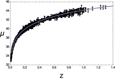
Figure 1: Background dynamics:Results of joint analysis by using $SNIa$ and $H(z)$ data. Here we have used $r_{0}=1/3$.

It is interesting to note that the parameter $\beta_{2}>\beta_{1}$ and that the present value for the EoS parameter $w_{0}$ is well supported by observational data C4 ; C5 . In spite that the model is in well-agreement with background data ($\chi^{2}_{\nu}\sim 1.12$), we will see in the next section, that the general model, together with its best-fit model, presents instabilities at perturbative level doing inviable the processes of structure formation and CMB anisotropies. In order to avoid the instabilities we can mention that it will be possible only reconstruct the model from an analysis of the perturbative dynamics. However, the reconstruction will have implications in the best-fit background model.

In the next section we will study the linear perturbations and instabilities for our interacting Ricci DE model.

VI Linear perturbations and instabilities: interacting Ricci dark energy model

In order to study the linear perturbations and the instabilities in our concrete example, we find that the perturbation, at linear order, of the interaction term $\delta Q^{c}$ can be written as

$$\delta Q^{c}=-{\epsilon_{m}}\left[aHv_{1}\delta^{c\prime}+g_{3}\delta^{c}+g_{4}S^{c}\right],$$ (62)

where the functions $g_{3}$ and $g_{4}$ are given by

$$g_{3}\equiv\frac{3H}{1+r+w}\left[q_{m}w-r(\beta_{1}-\beta_{2})\right]-3H\beta_{2},\,\,\mbox{and}\,\,g_{4}\equiv 3H\frac{r}{1+r+w}(\beta_{1}-\beta_{2})+3Hq_{m},$$

respectively. Here we have used Eqs.(25) and (52).

Now replacing Eq.(62) in Eq.(45), we obtain that the equation for $S^{c}$ becomes

$$S^{c\,\prime\prime}+\left(1+y_{3}+m\right)\frac{S^{c\,\prime}}{a}+\left(ay^{\prime}_{3}+y_{3}m+\frac{k^{2}y_{1}}{a^{2}H^{2}}\right)\frac{S^{c}}{a^{2}}=-\left[av^{\prime}_{3}+v_{3}m+\frac{k^{2}v_{1}}{a^{2}H^{2}}\left(\frac{\hat{c}^{2}_{s}}{q_{m}}-y_{1}\right)\right]\frac{\delta^{c}}{a^{2}}$$

$$-\left(v_{3}-v_{1}m-av^{\prime}_{1}-v_{1}\right)\frac{\delta^{c\,\prime}}{a}+v_{1}\delta^{c\,\prime\prime},$$ (63)

where

$$y_{3}=3y_{1}(1-q_{m})-\frac{3\,r(\beta_{1}-\beta_{2})}{1+r+w},\,\,\mbox{and}\,\,v_{3}=3v_{1}\left[y_{1}(q_{m}-1)-1-\hat{c}^{2}_{s}\right]+\frac{3(\beta_{2}+r\beta_{1}+w\beta_{2})}{1+r+w}\,.$$

Combining solutions of Eqs.(44) and (63) for our specific model we find that the matter density perturbation comoving to dark matter, results in

$$\delta^{c_{m}}_{m}=\frac{1+r}{1+r+w}\delta^{c}-S^{c}-3H^{2}(q_{m}-1)\frac{a^{2}}{k^{2}}\left(aS^{c\prime}+v_{3}\delta^{c}+y_{3}S^{c}-av_{1}\delta^{c\prime}\right),$$ (64)

and for the holographic Ricci dark energy density perturbation comoving to dark matter we get

$$\delta^{c_{m}}_{H}=\frac{w}{1+r+w}\delta^{c}+S^{c}+3H^{2}(1+r+w)\frac{a^{2}}{k^{2}}\left(aS^{c\prime}+v_{3}\delta^{c}+y_{3}S^{c}-av_{1}\delta^{c\prime}\right).$$ (65)

Here we have used Eq.(40).

In order to know the evolution of the perturbations $\delta^{c_{m}}_{m}$, it is necessary solve the system of equations given by (44)–(63). However, first we shall analyze the initial conditions of this perturbations considering the high-redshift limit.

.

VI.1 Analysis at High-redshifts and Comparing with $\Lambda$CDM

In the following we will analyze our results in high-redshift limit, in which $z\gg 1$ (or equivalently $a\ll 1$). At this limit we obtain that the expressions for the quantity $q_{m}$, given by Eq.(53), the rate $r$, and the EoS parameter $w$ from Eq.(54) become

$$q_{m}\rightarrow\frac{C\beta_{2}-D\beta_{1}}{C-D},\,\,\,\,\,r\rightarrow-\frac{D}{C},\,\,\mbox{and}\;\;\,w\rightarrow-\frac{D}{3C}-\frac{r_{0}}{3}+w_{0},\,\,\,\,\,(a\ll 1)$$ (66)

where $C$ and $D$ are given by Eq.(55). In particular, in the non-interacting case, i.e., $\beta_{1}=\beta_{2}=0$ where $C=1/3$ and $D=w_{0}-\frac{r_{0}}{3}$, we find that at high- redshift limit $q_{m}\rightarrow 0,\,\,\,\,\,r\rightarrow r_{0}-3w_{0},$ and $\,w\rightarrow 0$.

Figure 2: The evolution of the perturbation $\delta^{cm}_{m}$ versus the scale factor $a$, for three different scales $k$. Here we have considered the best fit values of our parameters in which $\beta_{1}=-0.05$, $\beta_{2}=0.18$ and $w_{0}=-0.95$, respectively.

On the other hand, we obtain that the Eq.(44) at high-redshift reduces to

$$\delta^{c\prime\prime}+c_{1}\frac{\delta^{c\prime}}{a}+c_{2}\frac{\delta^{c}}{a^{2}}=0,\;\;\,\,\,\,(a\ll 1),$$ (67)

where $c_{1}\approx\frac{3}{2}$ and $c_{2}\approx-\frac{3}{2}$. Here we have considered the value $r_{0}\approx\frac{1}{3}$ and the values of the best-fit: $\beta_{1}=-0.05$, $\beta_{2}=0.18$ and $w_{0}=-0.95$.

In particular for the non-interacting case ($\beta_{1}=\beta_{2}=0$), the Eq.(44) approaches exactly to the Einstein-de Sitter limit

$$\delta^{c\prime\prime}+\frac{3}{2a}\delta^{c\prime}-\frac{3}{2a^{2}}\delta^{c}=0,\,\,\,\,\,(a\ll 1).$$ (68)

Here we observe that Eqs.(67) and (68) are very similar, since the constants $c_{1}\approx-c_{2}\approx 2/3$ in Eq.(67).

Now considering Eq.(66), we find that the Eq.(63) at high-redshift becomes

$$S^{c\prime\prime}+c_{3}\frac{S^{c\prime}}{a}+c_{4}\frac{S^{c}}{a^{2}}+c_{5}\delta^{c\prime\prime}+c_{6}\frac{\delta^{c\prime}}{a}+c_{7}\frac{\delta^{c}}{a^{2}}=0,\,\,\,\,\,(a\ll 1),$$ (69)

where $c_{3}\approx\frac{3}{2}$ and $c_{4}\approx c_{5}\approx c_{6}\approx c_{7}\approx 0$. As before we have used the best -fit values.

For the non-interacting limit ($\beta_{1}=\beta_{2}=0$), we obtain

$$S^{c\prime\prime}+\frac{3}{2a}S^{c\prime}=0,\,\,\,\,\,(a\ll 1).$$ (70)

Again we note that Eqs.(69) and (70) are very similar for $S^{c\prime}$, since the constants $c_{4}\approx c_{5}\approx c_{6}\approx c_{7}\approx 0$. Also we observe that the solution of $S^{c}$ from Eq.(69) (or Eq. (70)) has two modes; one decaying solution (nonphysical) and the solution; $S^{c}$=constant. This last solution suggests that we could consider the adiabatic condition or equivalently $S^{c}\approx 0$ for the coupled system (see e.g., Ref.Hipolito2010 ).

In Fig.2 we show the evolution of $\delta^{cm}_{m}$ as a function of the scale factor $a$ for three different scales $k$. In order to write down values for the perturbation $\delta^{cm}_{m}$ and the scale factor, we solve numerically the Eqs. (44) and (63) by using the best fit values found in the previous section and adiabatic initial conditions. We observe that the behavior of $\delta^{cm}_{m}=\delta^{cm}_{m}(a)$ on different scales $k$ is similar. We also note that the perturbations slowly increase until approximately the value $a=1$ and then they start to oscillate before diverge. This instability occurs when the EoS parameter $w$ crosses the value $w=-1$ in its evolution, known as the phantom crossing , and then the perturbation collapses at this time and, in particular, at future values for the scale factor $a>1$.

It is interesting to compare our results for the matter perturbations of our holographic model with the behavior of the matter perturbations in $\Lambda$CDM model. Here we mention that the $\Lambda$CDM model can be obtained as a specific case of Eq.(44), since in this model the pressure $p=p_{\Lambda}=-\epsilon_{\Lambda}$=constant and then we have

$$\epsilon = \epsilon_{m}+\epsilon_{\Lambda},\,\,\,\;\;\;\frac{p}{\epsilon}=-\frac{\epsilon_{\Lambda}}{\epsilon_{\Lambda}+\epsilon_{m}}=-\frac{1}{1+r},$$

$$\mbox{and}\,\,\,\,\,r = r_{0}a^{-3}\,\,\,\,\,(\Lambda CDM).$$ (71)

In this form, Eq.(44) reduces to

$$\delta^{c\prime\prime}+\left[\frac{3}{2}-\frac{15}{2}\frac{p}{\epsilon}\right]\frac{\delta^{c\prime}}{a}-\left[\frac{3}{2}+12\frac{p}{\epsilon}-\frac{9}{2}\frac{p^{2}}{\epsilon^{2}}\right]\frac{\delta^{c}}{a^{2}}=0\,\,\,(\Lambda CDM).$$ (72)

Now considering that the perturbations $\delta\epsilon^{c}=\delta\epsilon_{m}^{c}$ since $\delta\epsilon_{\Lambda}=0$, we find that the relation between $\delta^{c}$ and $\delta^{c}_{m}$ can be written as

$$\delta^{c}=\frac{\delta\epsilon^{c}}{\epsilon}=\frac{\delta\epsilon_{m}^{c}}{\epsilon_{\Lambda}+\epsilon_{m}}=\delta_{m}^{c}\frac{r}{1+r}\,\,\,\,\,(\Lambda CDM),$$ (73)

and replacing this relation in Eq.(72) we obtain the standard expression for the matter energy perturbation given in $\Lambda CDM$ model

$$\delta_{m}^{c\prime\prime}+\frac{3}{2}\left(\frac{2+r}{1+r}\right)\frac{\delta_{m}^{c\prime}}{a}-\frac{3}{2}\left(\frac{r}{1+r}\right)\frac{\delta_{m}^{c}}{a^{2}}=0,\,\,\,\,\,(\Lambda CDM)$$ (74)

with the ratio $r=r(a)$ given by Eq.(71).

VII Avoiding instabilities and an appropriate model

In Sect. IV it was demonstrated that the perturbative dynamics of some dark energy models with a dynamical EoS parameter $w$ presents instabilities. The instabilities in the structure formation at linear regime are strongly related to the condition $1+w=0$ at finite time. In our analysis, the quantity $1+w$ appears in the coefficient $\tilde{A}$ of Eq.(30) and is hidden in the $\delta p^{c_{x}}$ term of function $\tilde{B}$ (see Eq. (43)). These are the sources of instabilities in the perturbative dynamics for any dark energy model with a dynamical EoS parameter $w$ with crossing phantom. As we noted, such perturbations become very large when the parameter $w$ approaches to $w\sim-1$. We also noted that this feature does not depend on the interaction term $Q$, since the quantity $1+w$ does not appear in the perturbation of the interaction term $\delta Q^{c}$.

In the following we will analyze the conditions for which the quantity $1+w$ becomes zero and study how to avoid this situation in our specific model, for any finite time.

From Eq.(54) we obtain that the quantity $1+w$ can be written as

$$1+w=\left[\frac{Dr_{0}-Cr_{0}\left(3w_{0}-r_{0}+3\right)+\left(3w_{0}-r_{0}+3\right)\left(Cr_{0}+D\right)a^{-3D}}{3\left(Cr_{0}+D\right)a^{-3D}-3Cr_{0}}\right]\,.$$ (75)

In order to avoid the instabilities we can consider that the quantity $1+w=0$ occurs for a determined value $a_{i}$ of the scale factor in Eq.(75), yielding

$$\left[Dr_{0}-Cr_{0}\left(3w_{0}-r_{0}+3\right)+\left(3w_{0}-r_{0}+3\right)\left(Cr_{0}+D\right)a^{-3D}\right]|_{a=a_{i}}=0\,,$$ (76)

in which for $a_{i}$ we get

$$a_{i}^{-3D}=\frac{Cr_{0}\left(3w_{0}-r_{0}+3\right)-Dr_{0}}{\left(3w_{0}-r_{0}+3\right)\left(Cr_{0}+D\right)}\,,$$ (77)

where $-3D=r_{0}-3w_{0}-\beta_{2}>0$. In order to evade the singularities in any finite time, we may considered that the scale factor $a_{i}\rightarrow\infty$ at a finite time in the future. In this form , from Eq.(77), we obtain that the condition $a_{i}\rightarrow\infty$ is satisfied in two cases; i) $Cr_{0}+D=0$ or ii) $3w_{0}-r_{0}=-3$. Analyzing separately for both cases we have that:

For the case in which $Cr_{0}+D=0$ (or equivalently $r_{0}=-(\beta_{2}+w_{0})/\beta_{1}$) we get

$$\frac{w}{1+r}=\frac{1}{3}\frac{D-C\left(3w_{0}-r_{0}\right)}{(D-C)}=\frac{w_{0}}{1+r_{0}}.$$ (78)

Now, replacing in Eq.(56) we find that the Hubble rate in terms of the scale factor $a$ becomes

$$H=H_{0}a^{-\frac{3}{2}\left(1+\frac{w_{0}}{1+r_{0}}\right)}\,\,\,\,\;\;\;\mbox{in which}\;\;\;\;\,\,\,\,a(t)\propto t^{\frac{2}{3(1+w_{0}/(1+r_{0}))}}.$$ (79)

Here, we note that this Hubble rate does not depend on the parameters which characterize the interaction term. We also note that this expression for the Hubble rate describes an universe without an acceleration phase in the case $1+r_{0}>-w_{0}$, then the model is disproved from observations. The acceleration phase occurs when $1+r_{0}<-w_{0}$, however this condition corresponds to phantom model, since $r_{0}>0$ then $w_{0}<-1$ and the instabilities take place at values for the scale factor such that $a_{i}<1$ (past time), then we discarded this phantom model. In this way, the first condition $Cr_{0}+D=0$ is not a suitable condition to avoid the instabilities.

Now let us analyze the second condition $3w_{0}-r_{0}=-3$. From this condition we note that the values $r_{0}$ and $w_{0}$ cannot be taken independently. Also, we note that as $r_{0}>0$ then the parameter $w_{0}>-1$. Considering the second condition we get that the parameter which characterizes the Ricci DE, $c^{2}$, becomes $c^{2}=2(r_{0}-3w_{0}+1)^{-1}=1/2$, independently of the values of $r_{0}$ and $w_{0}$. This result for the parameter $c^{2}=1/2$ of the Ricci DE coincides with the obtained in Refs.DelCampo2013 ; V0 from the analysis of the non-interacting case, where the instabilities in the non-adiabatic perturbations were considered.

As before we obtain that the quantity $1+w$ as a function of the scale factor becomes

$$1+w=1+\frac{Dr_{0}+3Cr_{0}-3\left(Cr_{0}+D\right)a^{-3D}}{3\left(Cr_{0}+D\right)a^{-3D}+3(D-C)r_{0}}=\frac{4Dr_{0}}{3\left(Cr_{0}+D\right)a^{-3D}+3(D-C)r_{0}}\,,$$ (80)

and from Eq.(56), the solution for the Hubble rate becomes

$$H=H_{0}a^{-3/2}\left[\frac{\left(Cr_{0}+D\right)a^{-3D}+\left(D-C\right)r_{0}}{D(1+r_{0})}\right]^{-1/2D}\,,$$ (81)

or equivalently

$$H=H_{0}a^{-3/2}\left[\left(1+\frac{3(\beta_{1}-\beta_{2})+4}{3(\beta_{2}-1)}\Omega_{m0}\right)\,a^{-3(\beta_{2}-1)}-\frac{3(\beta_{1}-\beta_{2})+4}{3(\beta_{2}-1)}\Omega_{m0}\right]^{-\frac{1}{2(\beta_{2}-1)}}.$$ (82)

Here we have used that $1=\Omega_{m0}+\Omega_{H0}$, then $\Omega_{m0}=3(1+w_{0})/[1+3(1+w_{0})]$.

Figure 3: Model without instabilities: Results of joint analysis by using SNIa and $H(z)$ data considering the second condition. Here we have considered Eq.(83) and $\Omega_{m0}=0.25$.

As before, we perform the same analysis of section V, considering the SNIa and $H(z)$ data sets. In Fig.(3) we show the constraints on the $\beta_{1}-\beta_{2}$ plane after marginalization in the parameter $\Omega_{m0}$ and the constraints on the $\beta_{2}-\Omega_{m0}$ plane after marginalization in the parameter $\beta_{1}$, considering Eq.(83). Again the lines represent the contours of the 1$\sigma$, 2$\sigma$ and 3$\sigma$ regions, respectively. We find that the values of the best-fit for the parameters $\beta_{1}$, $\beta_{2}$ and $\Omega_{m0}$ become $\beta_{1}=-0.03^{+0.04+0.07+0.08}_{-0.10-0.14-0.17}$, $\beta_{2}=0.22^{+0.09+0.14+0.18}_{-0.10-0.14-0.17}$, and $\Omega_{m0}=0.25^{+0.01+0.03+0.04}_{-0.01-0.02-0.03}$, respectively ($\chi^{2}_{\nu}\sim 1.17$). We note a drastic change in the values of the parameters in order to avoid the appearance of instabilities in the perturbative dynamics. We also note that form the best-fit, $\beta_{1}>\beta_{2}$, then the direction of energy transfer is from DE to DM, since $q_{m}>0$, or equivalently $Q>0$ (figure not shown). In particular, the value $\beta_{1}$ changes from $\beta_{1}=-0.05$ to $\beta_{1}=-0.03$, which represents an increase about of 40 percent, and for $\beta_{2}$ an increase about of 22$\%$.

In Fig.(4) we show the plot of the luminosity distance $\mu$ versus the redshift $z$ for the best-fit values in contrast with JLA SNIa data and considering the second condition $3w_{0}-r_{0}=-3$. Here we have used the values $\beta_{1}=-0.03$, $\beta_{2}=0.22$ and $\Omega_{m0}=0.25$ (best-fit values avoiding instabilities). We note that the solution of the Hubble rate, given by Eq.(83), presents an accelerate phase and is well supported by the observational data.

On the other hand, it is interesting to compare our model with the holographic Ricci DE model without DE-DM interaction, considering the reduced chi square $\chi^{2}_{\nu}$ statistical function with the same data set. In this form, we could determine which type of model best fits to the observation data, observing that model presents the lowest value of $\chi_{\nu}^{2}$. In the case without DE-DM interaction, the Hubble rate for the model without instabilities is given by DelCampo2013

$$H=H_{0}\left[\left(1-\frac{4}{3}\Omega_{m0}\right)\,+\frac{4}{3}\Omega_{m0}\,a^{-3}\right]^{\frac{1}{2}}.$$ (83)

Here, we note that we have only one free parameter, the matter density $\Omega_{m0}$. By performing joint tests using JLA SNIa and $H(z)$ data set we obtain that $\Omega_{m0}=0.22^{+0.01+0.03+0.04}_{-0.01-0.03-0.04}$ with $\chi^{2}_{\nu}\sim 1.18$. However, we observe that this goodness-of-fit is slightly higher than the case with interaction, since we have found the value $\chi^{2}_{\nu}\sim 1.17$. Unfortunately, because of the similitude in the values of $\chi^{2}_{\nu}$ obtained in both models, we cannot directly deduce which model realizes better the observational data. Strictly, our model presents a lower value in relation to the non-interacting model, then we may conclude that the most general case with energy transfer between DE-DM is well suited for to study and is well confronted with the observational data.

Figure 4: Model without instabilities: Plot of the luminosity distance $\mu$ versus the redshift $z$ for the best-fit values in contrast with JLA SNIa data and considering the second condition i.e., $3w_{0}-r_{0}=-3$. Here we have used the values $\beta_{1}=-0.03$, $\beta_{2}=0.22$.

In Figs.(5) and (6) we show the evolution of the perturbation $\delta^{cm}_{m}$ as a function of the scale factor $a$ for two different scales $k$: $k=0.05h^{-1}Mpc^{-1}$ and $k=1.5h^{-1}Mpc^{-1}$, respectively. Here, we have denoted as the Model 1 the model with instabilities and the Model 2 as the model without instabilities considering the second condition $3w_{0}-r_{0}=-3$ . As before, we find numerically the solutions for the coupled system Eqs. (44) and (63) by considering the best fit values found from the data analysis for both models, see Figs. (1) and (3). Here we have used the values $\beta_{1}=-0.05$, $\beta_{2}=0.18$ and $w_{0}=-0.95$ for the model 1, and $\beta_{1}=-0.03$, $\beta_{2}=0.22$ and $\Omega_{m0}=0.25$ for the model 2. We observe that by considering the second condition $3w_{0}-r_{0}=-3$ (model 2), we can evade the instabilities in the structure formation and then we obtain an appropriate model for the dark sector from the perturbative analysis.

Figure 5: The evolution of the perturbation $\delta^{cm}_{m}$ as function of the scale factor $a$, for the scale $k=0.05h^{-1}Mpc^{-1}$. Here we have used the values $\beta_{1}=-0.05$, $\beta_{2}=0.18$ and $w_{0}=-0.95$ for the model 1, and $\beta_{1}=-0.03$, $\beta_{2}=0.22$ and $\Omega_{m0}=0.25$ for the model 2.

VIII Conclusions

Figure 6: The evolution of the perturbation $\delta^{cm}_{m}$ as function of the scale factor $a$, for the scale $k=1.5h^{-1}Mpc^{-1}$. Here we have used the values $\beta_{1}=-0.05$, $\beta_{2}=0.18$ and $w_{0}=-0.95$ for the model 1, and $\beta_{1}=-0.03$, $\beta_{2}=0.22$ and $\Omega_{m0}=0.25$ for the model 2.

In this paper we have analyzed an interacting model of dark energy and dark matter in order to describe of late cosmic acceleration of the universe. Under a general formalism we have described the perturbative dynamics for these two interacting fluids. In this general analysis we have considered the timelike part of the balance equation, the momentum balance and the momentum transfer $Q^{\alpha}$ associated to the interaction term $Q$. From the functions of contrast for dark matter and dark energy we have studied the perturbative dynamics considering a gauge-invariant treatment in comoving gauge. On the other hand, we have obtained the total non-adiabatic and dark energy pressure perturbations and we found the relation between these gauge-invariant quantities. Also, we have identified the sources of instabilities in DE models with a dynamical EoS parameter that presents a phantom crossing. As a concrete example we have considered an interaction term $Q$ between the holographic Ricci-DE and DM. Here we have studied that the interaction term $Q$, depends on the energy densities of both components multiplied by a quantity with units of the inverse of time (proportional to the Hubble parameter). From the background equations we have obtained the constraints on the parameters characterizing the interaction by considering the observational analysis from the SNIa and $H(z)$ tests. Here from the background dynamics we have found that the best-fit values for the parameters of the interaction are $\beta_{1}=-0.05^{+0.05+0.08+0.10}_{-0.05-0.07-0.09}$, $\beta_{2}=0.18^{+0.04+0.06+0.08}_{-0.04-0.06-0.08}$, and for the EOS parameter $w_{0}=-0.95^{+0.05+0.06+0.08}_{-0.05-0.07-0.09}$. In our perturbative analysis we have found that, in this best-fit model, the instabilities appear at the moment when the EoS parameter $w$ crosses the value $w\sim-1$ and we have noted that this feature does not depend on the interaction term $Q$. In order to avoid these instabilities in the perturbative analysis and develop an appropriate model for any finite time, we have obtained a specific value of the scale factor denoted as $a_{i}$. From this value of $a_{i}$ we have obtained two independent conditions to avoid the instabilities in our specific model, namely: i) $Cr_{0}=-D$ and ii) $r_{0}=3(w_{0}+1)$. Considering the first condition we have found that if $w_{0}<1+r_{0}$, the model is disproved from observations, since under this requirement the model does not present an accelerate scenario. Otherwise if $w_{0}>1+r_{0}$, we have obtained an accelerate phase, however this condition corresponds to a phantom model, nothing that the instabilities take place in the past time. In this way, we have obtained that the first condition is not suitable. From the second condition i.e., $r_{0}=3(w_{0}+1)$, we have found an accelerate phase of the universe and also corresponds to an appropriate model for any finite time. In order to avoid the instabilities in the perturbative dynamics, we have noted that this result agrees with obtained in Ref.DelCampo2013 and becomes independently of the interaction term. Moreover we have obtained that the constraint on the Ricci parameter $c^{2}=1/2$ is fixed for the second condition, since as from background $c^{2}=2(r_{0}-3w_{0}+1)^{-1}$ and together the second condition $r_{0}=3(w_{0}+1)$, then $c^{2}=1/2$, independency of the values $r_{0}$ , $w_{0}$ and the energy transfer rate $Q$. Also, from this condition we have found, in order to have an appropriate model, a new sets of best-fit values for the interaction parameters given by $\beta_{1}=-0.03^{+0.04+0.07+0.08}_{-0.10-0.14-0.17}$, $\beta_{2}=0.22^{+0.09+0.14+0.18}_{-0.10-0.14-0.17}$, and $\Omega_{m0}=0.25^{+0.01+0.03+0.04}_{-0.01-0.02-0.03}$. Here we have observed a drastic change in the values of the parameters $\beta_{1}$ and $\beta_{2}$ in order to avoid the singularity from the perturbative dynamics. For the parameter $\beta_{1}$ we have found that the increased is the order of 40$\%$ and for $\beta_{2}$ is the order of 22$\%$.

Finally, we would like to point out that in models that have a phantom crossing, and in particular for the holographic models (with and without interaction), it is necessary to be cautious when only the background level observational tests are being considered. Here, we have shown that in spite of a good agreement with data and an adequate background dynamic, this could lead to inviable models at perturbative level.

IX Acknowledgments

R. H. was supported by Comisión Nacional de Ciencias y Tecnología of Chile through FONDECYT REGULAR Grant N₀ 1130628 and DI-PUCV 123.724. N. V. was supported by Comisión Nacional de Ciencias y Tecnología of Chile through FONDECYT Grant N₀ 3150490. WSHR was supported by Brazilian agencies CAPES (proccess No 99999.007393/2014-08) at the begining of this work, and FAPES at the end (BPC No 476/2013). WSHR is grateful for the hospitality of the Physics Department of McGill University where part of this work was developed.

References

- (1) A. Riess et al., Astron. J. 116, 1009 (1998).
- (2) S. Permutter et al., Astron. J. 517, 565 (1999).
- (3) M. Tegmark et al., Astron. J. 606, 702 (2004).
- (4) P. A. R. Ade et al., Astron. Astrophys. A16, 571 (2014); N. Aghanim et al. [Planck Collaboration], [arXiv:1507.02704 [astro-ph.CO]].
- (5) P. A. R. Ade et al. [Planck Collaboration], doi:10.1051/0004-6361/201525941 arXiv:1502.01591 [astro-ph.CO]; P. A. R. Ade et al. [Planck Collaboration], arXiv:1502.01589 [astro-ph.CO].
- (6) L. Amendola, Phys. Rev. D 62, 043511 (2000); L. Amendola and C. Quercellini, Phys. Rev. D 68, 023514 (2003); L. Amendola, S. Tsujikawa, and M. Sami, Phys. Lett. B 632, 155 (2006).
- (7) D. Pavon, W. Zimdahl, Phys. Lett. B 628, 206 (2005); S. Campo, R. Herrera, D. Pavon, Phys. Rev.D 78, 021302(R) (2008).
- (8) B. Wang, J. Zang, C.-Y. Lin, E. Abdalla, and S. Micheletti, Nucl. Phys. B 778, 69 (2007); S. Cao and N. Liang, Int. J. Mod. Phys. D 22 (2013).
- (9) Z. K. Guo, N. Ohta, and S. Tsujikawa, Phys. Rev. D 76, 023508 (2007); M. Le Delliou, R. Marcondes, G. Lima Neto, and E. Abdalla, Mon. Not. Roy. Astron. Soc. 453, 2 (2015); B. Wang, E. Abdalla, F. Atrio-Barandela and D. Pavon, arXiv:1603.08299 [astro-ph.CO].
- (10) W. Zimdahl and D. Pavon, Gen. Rel. Grav. 36, 1483 (2004); O. Bertolami, F. Gil Pedro and M. Le Delliou, Phys. Lett. B 654, 165 (2007).
- (11) W. Zimdahl, Int. J. Mod. Phys. D 14, 2319 (2005); R. G. Cai and A. Wang, JCAP 0503, 002 (2005); L. Amendola, G. Camargo Campos and R. Rosenfeld, Phys. Rev. D 75, 083506 (2007); G. Caldera-Cabral, R. Maartens and L. A. Urena-Lopez, Phys. Rev. D 79, 063518 (2009).
- (12) C. G. Park, J. C. Hwang, J. H. Lee, and H. Noh, Phys. Rev. Lett. 103, 151303 (2009).
- (13) R. Bean and O. Dore, Phys. Rev. D 69, 083503 (2004);
- (14) J. Weller and A. M. Lewis, Mon. Not. Roy. Astron. Soc. 346, 987 (2003);
- (15) G. B. Zhao, J. Q. Xia, M. Li, B. Feng, and Xinmin Zhang, Phys. Rev. D 72, 123515 (2005),
- (16) R. Bean, E. Flanagan and M. Trodden, Phys. Rev. D 78, 023009 (2008).
- (17) J. Valiviita , E. Majerotto and R. Maartens, J. Cosmol. Astropart. Phys. 07, 020 (2008).
- (18) M. Kunz and D. Sapone, Phys. Rev. D 74, 123503 (2006).
- (19) L. Susskind, J. Math. Phys. 36, 6377 (1995); J. M. Maldacena, Adv. Theor. Math. Phys. 2, 231 (1998); R. Bousso, Rev. Mod. Phys. 74, 825 (2000).
- (20) A. G. Cohen, D.B. Kaplan and A.E. Nelson, Phys. Rev. Lett. 82, 4971 (1999);
- (21) M. Li, Phys. Lett. B 603, 1 (2004).
- (22) S. Nojiri, S. D. Odintsov, Gen.Rel.Grav. 38 1285 (2006).
- (23) B. Wang, Y. g. Gong and E. Abdalla, Phys. Lett. B 624, 141 (2005); B. Wang, C. Y. Lin and E. Abdalla, Phys. Lett. B 637, 357 (2006); M. R. Setare, Eur. Phys. J. C 50, 991 (2007) ; R. C. G. Landim, Int.J.Mod.Phys. D 25, No. 4 1650050 (2016).
- (24) H. Kim, H. W. Lee and Y. S. Myung, Phys. Lett. B 632, 605 (2006).
- (25) W. Zimdahl and D. Pavon, Class. Quant. Grav. 24, 5461 (2007); Q. Wu, Y. Gong, A. Wang and J. S. Alcaniz, Phys. Lett. B 659, 34 (2008); J. Zhang, H. Liu and X. Zhang, Phys. Lett. B 659, 26 (2008); A. A. Sen and D. Pavon, Phys. Lett. B 664, 7 (2008); I. Duran, D. Pavon and W. Zimdahl, JCAP 1007, 018 (2010); K. Das and T. Sultana, Astrophys. Space Sci. 361, no. 2, 53 (2016).
- (26) R. Brustein and G. Veneziano, Phys. Rev. Lett. 84, 5695 (2000).
- (27) C. Gao, F. Q. Wu, X. Chen, and Y. G. Shen, Phys. Rev. D 79, 043511 (2009).
- (28) C. J. Feng, Phys. Lett. B 670, 231 (2008); X. Zhang, Phys. Rev. D 79, 103509 (2009); L. Xu and Y. Wang, JCAP 1006, 002 (2010); M. Suwa and T. Nihei, Phys. Rev. D 81, 023519 (2010).
- (29) K. Karwan and T. Thitapura, JCAP 1201, 017 (2012);
- (30) Yuting Wang, Lixin Xu and Yuanxing Gui, Phys. Rev. D 84, 063513 (2011); Chao-Jun Feng and Xin-Zhou Li, Phys. Lett. B680, 355 (2009).
- (31) S. del Campo, J. C. Fabris, R. Herrera and W. Zimdahl, Phys. Rev. D 87, no. 12, 123002 (2013).
- (32) J. Bardeen, Phys. Rev D 22, 1882 (1996).
- (33) W.S.Hipólito-Ricaldi, H.E.S. Velten and W. Zimdahl, JCAP, 06, 016 (2009).
- (34) A.Romero Fuño, W.S. Hipólito-Ricaldi and W. Zimdahl, MNRAS 57 no.3, 2958 (2016).
- (35) R.F. vom Marttens, W.S. Hipólito-Ricaldi and W. Zimdahl, JCAP, 08, 004 (2014).
- (36) H. Kodama and M. Sasaki, Prog. Theor. Phys. Suppl. 78, 1 (1984).
- (37) K. A. Malik, D. Wands and C. Ungarelli, Phys. Rev. D 67, 063516 (2003).
- (38) C. Zuñiga-Vargas, W.S. Hipólito-Ricaldi and W. Zimdahl, JCAP, 04, 032 (2012).
- (39) W. S. Hipolito-Ricaldi, H. E. S. Velten and W. Zimdahl, Phys. Rev. D 82, 063507 (2010).
- (40) S. del Campo, J.C. Fabris, R. Herrera and W. Zimdahl, Phys.Rev.D 83, 123006 (2011).
- (41) G. R. Farrar and P. J. E. Peebles, Astrophys. J. 604, 1 (2004); S. del Campo, R. Herrera and D. Pavon, Phys. Rev. D 70, 043540 (2004); R. Herrera, D. Pavon and W. Zimdahl, Gen. Rel. Grav. 36, 2161 (2004); S. del Campo, R. Herrera, G. Olivares and D. Pavon, Phys. Rev. D 74, 023501 (2006); Phys. Rev. D 75, 083506 (2007); S. del Campo, R. Herrera and D. Pavon, Int. J. Mod. Phys. D 20, 561 (2011).
- (42) M.S. Turner, Phys. Rev. D 28, 1243 (1983).
- (43) H. Wei and R. G. Cai, Eur. Phys. J. C 59, 99 (2009); H. M. Sadjadi and M. Alimohammadi, Phys. Rev. D 74, 103007 (2006); A. Sheykhi, Phys. Lett. B 681, 205 (2009); R. Herrera and N. Videla, Int. J. Mod. Phys. D 23, no. 08, 1450071 (2014); M. Szydłowski, A. Krawiec, A. Kurek and M. Kamionka, Eur. Phys. J. C 75, no. 99, 5 (2015); S. del Campo, R. Herrera and D. Pavón, Phys. Rev. D 91, no. 12, 123539 (2015).
- (44) M. Betoule et. al., Astron. Astrophys. 568, A22 (2014) .
- (45) O. Farooq, B. Ratra, Astrophys.J.. 766. L7 (2013).
- (46) http://supernovae.in2p3.fr/sdss_snls_jla/ReadMe.html.
- (47) J. Simon, L. Verde and R. Jimenez, , Phys. Rev. D 71 (2005) 123001 [arXiv:0412269].
- (48) D. Stern, R. Jimenez, L. Verde, M. Kamionkowski and S.A. Stanford, J. Cosmol. Astropart. Phys. 02, 008 (2010) . .