Approximate Bayesian Computation in Large Scale Structure: constraining the galaxy-halo connection
Abstract
Standard approaches to Bayesian parameter inference in large scale structure assume a Gaussian functional form (chi-squared form) for the likelihood. This assumption, in detail, cannot be correct. Likelihood free inferences such as Approximate Bayesian Computation (ABC) relax these restrictions and make inference possible without making any assumptions on the likelihood. Instead ABC relies on a forward generative model of the data and a metric for measuring the distance between the model and data. In this work, we demonstrate that ABC is feasible for LSS parameter inference by using it to constrain parameters of the halo occupation distribution (HOD) model for populating dark matter halos with galaxies.
Using specific implementation of ABC supplemented with Population Monte Carlo importance sampling, a generative forward model using HOD, and a distance metric based on galaxy number density, two-point correlation function, and galaxy group multiplicity function, we constrain the HOD parameters of mock observation generated from selected “true” HOD parameters. The parameter constraints we obtain from ABC are consistent with the “true” HOD parameters, demonstrating that ABC can be reliably used for parameter inference in LSS. Furthermore, we compare our ABC constraints to constraints we obtain using a pseudo-likelihood function of Gaussian form with MCMC and find consistent HOD parameter constraints. Ultimately our results suggest that ABC can and should be applied in parameter inference for LSS analyses.
keywords:
Large scale structure – cosmology – statistic1 Introduction
Cosmology was revolutionized in the 1990s with the introduction of likelihoods—probabilities for the data given the theoretical model—for combining data from different surveys and performing principled inferences of the cosmological parameters (White & Scott 1996; Riess et al. 1998). Nowhere has this been more true than in cosmic microwave background (CMB) studies, where it is nearly possible to analytically evaluate a likelihood function that involves no (or minimal) approximations (Oh et al. 1999, Wandelt et al. 2004, Eriksen et al. 2004, Planck Collaboration et al. 2014, 2015a).
Fundamentally, the tractability of likelihood functions in cosmology flows from the fact that the initial conditions are exceedingly close to Gaussian in form (Planck Collaboration et al. 2015b, c), and that many sources of measurement noise are also Gaussian (Knox 1995; Leach et al. 2008). Likelihood functions are easier to write down and evaluate when things are closer to Gaussian, so at large scales and in the early universe. Hence likelihood analyses are ideally suitable for CMB data.
In large-scale structure (LSS) with galaxies, quasars, and quasar absorption systems as tracers, formed through nonlinear gravitational evolution and biasing, the likelihood cannot be Gaussian. Even if the initial conditions are perfectly Gaussian, the growth of structure creates non-linearities which are non-Gaussian (see Bernardeau et al. 2002 for a comprehensive review). Galaxies form within the density field in some complex manner that is modeled only effectively (Dressler 1980; Kaiser 1984; Santiago & Strauss 1992; Steidel et al. 1998; see Somerville & Davé 2015 for a recent review). Even if the galaxies were a Poisson sampling of the density field, which they are not (Mo & White 1996; Somerville et al. 2001; Casas-Miranda et al. 2002), it would be tremendously difficult to write down even an approximate likelihood function (Ata et al. 2015).
The standard approach makes the strong assumption that the likelihood function for the data can be approximated by a pseudo-likelihood function that is a Gaussian probability density in the space of the two-point correlation function estimate. It is also typically limited to (density and) two-point correlation function (2PCF) measurements, assuming that these measurements constitute sufficient statistics for the cosmological parameters. As Hogg (in preparation) demonstrates, the assumption of a Gaussian pseudo-likelihood function cannot be correct (in detail) at any scale, since a correlation function, being related to the variance of a continuous field, must satisfy non-trivial positive-definiteness requirements. These requirements truncate function space such that the likelihood in that function space could never be Gaussian. The failure of this assumption becomes more relevant as the correlation function becomes better measured, so it is particularly critical on intermediate scales, where neither shot noise nor cosmic variance significantly influence the measurement.
Fortunately, these assumptions are not required for cosmological inferences, because high-precision cosmological simulations can be used to directly calculate LSS observables. Therefore, we can simulate not just the one- or two-point statistics of the galaxies, but also any higher order statistics that might provide additional constraining power on a model. In principle, there is therefore no strict need to rely on these common but specious analysis assumptions as it is possible to calculate a likelihood function directly from simulation outputs.
Of course, any naive approach to sufficiently simulating the data would be ruinously expensive. Fortunately, there are principled, (relatively) efficient methods for minimizing computation and delivering correct posterior inferences, using only a data simulator and some choices about statistics. In the present work, we use Approximate Bayesian Computation—ABC—which provides a rejection sampling framework (Pritchard et al. 1999) that relaxes the assumptions of the traditional approach.
ABC approximates the posterior probability distribution function (model given the data) by drawing proposals from the prior over the model parameters, simulating the data from the proposals using a forward generative model, and then rejecting the proposals that are beyond a certain threshold “distance” from the data, based on summary statistics of the data. In practice, ABC is used in conjunction with a more efficient sampling operation like Population Monte Carlo (PMC; Del Moral et al. 2006). PMC initially rejects the proposals from the prior with a relatively large “distance” threshold. In subsequent steps, the threshold is updated adaptively, and samples from the proposals that have passed the previous iteration are subjected to the new, more stringent, threshold criterion (Beaumont et al. 2009). In principle, the distance metric can be any positive definite function that compares various summary statistics between the data and the simulation.
In the context of astronomy, this approach has been used in a wide range of topics including image simulation calibration for wide field surveys (Akeret et al. 2015), the study of the morphological properties of galaxies at high redshifts (Cameron & Pettitt 2012), stellar initial mass function modeling (Cisewski et al. in preparation), and cosmological inference with with weak-lensing peak counts (Lin & Kilbinger 2015; Lin et al. 2016), Type Ia Supernovae (Weyant et al. 2013), and galaxy cluster number counts (Ishida et al. 2015).
In order to demonstrate that ABC can be tractably applied to parameter estimation in contemporary LSS analyses, we narrow our focus to inferring the parameters of a Halo Occupation Distribution (HOD) model. The foundation of HOD predictions is the halo model of LSS, that is, collapsed dark matter halos are biased tracers of the underlying cosmic density field (Press & Schechter 1974; Bond et al. 1991; Cooray & Sheth 2002). The HOD specifies how the dark matter halos are populated with galaxies by modeling the probability that a given halo hosts galaxies subject to some observational selection criteria (Lemson & Kauffmann 1999; Seljak 2000; Scoccimarro et al. 2001; Berlind & Weinberg 2002; Zheng et al. 2005). This statistical prescription for connecting galaxies to halos has been remarkably successful in reproducing the galaxy clustering, galaxy–galaxy lensing, and other observational statistics (Rodríguez-Torres et al. 2015; Miyatake et al. 2015), and is a useful framework for constraining cosmological parameters (van den Bosch et al. 2003; Tinker et al. 2005; Cacciato et al. 2013; More et al. 2013) as well as galaxy evolution models (Conroy & Wechsler 2009; Tinker et al. 2011; Leauthaud et al. 2012; Behroozi et al. 2013b; Tinker et al. 2013, Walsh et al. in preparation).
More specifically, we limit our scope to a likelihood analysis of HOD model parameter space, keeping cosmology fixed. We forward model galaxy survey data by populating pre-built dark matter halo catalogs obtained from high resolution N-body simulations (Klypin et al. 2011; Riebe et al. 2011) using 111http://halotools.readthedocs.org (Hearin et al. 2016a), an open-source package for modeling the galaxy-halo connection. Equipped with the forward model, we use summary statistics such as number density, two-point correlation function, galaxy group multiplicity function (GMF) to infer HOD parameters using ABC.
In Section 2 we discuss the algorithm of the ABC-PMC prescription we use in our analyses. This includes the sampling method itself, the HOD forward model, and the computation of summary statistics. Then in Section 3.1, we discuss the mock galaxy catalog, which we treat as observation. With the specific choices of ABC-PMC ingredients, which we describe in Section 3.2, in Section 3.3 we present the results of our parameter inference using two sets of summary statistics, number density and 2PCF and number density and GMF. We also include in our results, analogous parameter constraints from the standard MCMC approach, which we compare to ABC results in detail, Section 3.4. Finally, we discuss and conclude in Section 4.
2 Methods
2.1 Approximate Bayesian Computation
ABC is based on rejection sampling, so we begin this section with a brief overview of rejection sampling. Broadly speaking, rejection sampling is a Monte Carlo method used to draw samples from a probability distribution, , which is difficult to directly sample. The strategy is to draw samples from an instrumental distribution that satisfies the condition for all where is some scalar multiplier. The purpose of the instrumental distribution is that it is easier to sample than (see Bishop 2007 and refernces therein).
In the context of simulation-based inference, the ultimate goal is to sample from the joint probability of a simulation and parameters given observed data , the posterior probability distribution. From Bayes rule this posterior distribution can be written as
| (1) |
where is the prior distribution over the parameters of interest and is the evidence,
| (2) |
where the domain of the integral is all possible values of and . Since cannot be directly sampled, we use rejection sampling with instrumental distribution
| (3) |
and the choice of
| (4) |
Note that we do not ever need to know . The choices of and satisfy the condition
| (5) |
so we can sample by drawing from . In practice, this is done by first drawing from the prior and then generating a simulation via the forward model. Then is accepted if
| (6) |
where is drawn from . By repeating this rejection sampling process, we sample the distribution with the set of and that are accepted.
At this stage, ABC distinguishes itself by postulating that , the probability of observing data given simulation (not the likelihood), is proportional to the probability of the distance between the data and the simulation X being less than an arbitrarily small threshold
| (7) |
where is the distance between the data and simulation . Eq. 7 along with the rejection sampling acceptance criteria (Eq. 6), leads to the acceptance criteria for ABC: is accepted if .
The distance function is a positive definite function that measures the closeness of the data and the simulation. The distance can be a vector with multiple components where each component is a distance between a single summary statistic of the data and that of the simulation. In that case, the threshold in Eq. 7 will also be a vector with the same dimensions. is accepted if the distance vector is less than the threshold vector for every component.
The ABC procedure begins, in the same fashion as rejection sampling, by drawing from the prior distribution . The simulation is generated from using the forward model, . Then the distance between the data and simulation, , is calculated and compared to . If , is accepted. This process is repeated until we are left with a sample of that all satisfy the distance criteria. This final ensemble approximates the posterior probability distribution .
As it is stated, the ABC method poses some practical challenges. If the threshold is arbitrarily large, the algorithm essentially samples from the prior . Therefore a sufficiently small threshold is necessary to sample from the posterior probability distribution. However, an appropriate value for the threshold is not known a priori. Yet, even if an appropriate threshold is selected, a small threshold requires the entire process to be repeated for many draws of from until a sufficient sample is acquired. This often presents computation challenges.
We overcome some of the challenges posed by the above ABC method by using a Population Monte Carlo (PMC) algorithm as our sampling technique. PMC is an iterative method that performs rejection sampling over a sequence of distributions ( for iterations), with a distance threshold that decreases at each iteration of the sequence.
As illustrated in Algorithm 1, for the first iteration , we begin with an arbitrarily large distance threshold . We draw (hereafter referred to as particles) from the prior distribution . We forward model the simulation , calculate the distance , compare this distance to , and then accept or reject the draw. Because we set arbitrarily large, the particles essentially sample the prior distribution. This process is repeated until we accept particles. We then assign equal weights to the particles: .
For subsequent iterations () the distance threshold is set such that for all components . Although there is no general prescription, the distance threshold can be assigned based on the empirical distribution of the accepted distances of the previous iteration, . In Weyant et al. 2013, for instance, the threshold of the second iteration is set to the percentile of the distances in the first iterations; afterwards in the subsequent iterations, , is set to the percentile of the distances in the previous iteration. Alternatively, Lin & Kilbinger 2015 set to the median of the distances from the previous iteration. In Section 3, we describe our prescription for the distance threshold, which follows Lin & Kilbinger 2015.
Once is set, we draw a particle from the previous weighted set of particles . This particle is perturbed by a kernel, set to the covariance of . Then once again, we generate a simulation by forward modeling , calculate the distance , and compare the distance to the new distance threshold () in order to accept or reject the particle. This process is repeated until we assemble a new set of particles . We then update the particle weights according to the kernel, the prior distribution, and the previous set of weights, as described in Algorithm 1. The entire procedure is then repeated for the next iteration, .
There are a number of ways to specify the perturbation kernel in the ABC-PMC algorithm. A widely used technique is to define the perturbation kernel as a multivariate Gaussian centered on the weighted mean of the particle population with a covariance matrix set to the covariance of the particle population. This perturbation kernel is often called the global multivariate Gaussian kernel. For a thorough discussion of various schemes for specifying the perturbation kernel, we refer the reader to Filippi et al. 2011.
The iterations continue in the ABC-PMC algorithm until convergence is confirmed. One way to ensure convergence is to impose a threshold for the acceptance ratio, which is measured in each iteration. The acceptance ratio is the ratio of the number of proposals accepted by the distance threshold, to the full number of proposed particles at every step. Once the acceptance ratio for an iteration falls below the imposed threshold, the algorithm has converged and is suspended. Another way to ensure convergence is by monitoring the fractional change in the distance threshold () after each iteration. When the fractional change becomes smaller than some specified tolerance level, the algorithm has reached convergence. Another convergence criteria, is through the derived uncertainties of the inferred parameters measured after each iteration. When the uncertainties stabilize and show negligible variations, convergence is ensured. In Section 3.2 we detail the specific convergence criteria used in our analysis.
2.2 Forward model
2.2.1 Halo Occupation Modeling
ABC requires a forward generative model. In large scale structure studies, this implies a model that is able to generate a galaxy catalog. We then calculate and compare summary statistics of the data and model catalog in an identical fashion In this section, we describe the forward generative model we use within the framework of the halo occupation distribution.
The assumption that galaxies reside in dark matter halos is the bedrock underlying all contemporary theoretical predictions for galaxy clustering. The Halo Occupation Distribution (HOD) is one of the most widely used approaches to characterizing this galaxy-halo connection. The central quantity in the HOD is , the probability that a halo of mass hosts galaxies.
The most common technical methods for estimating the theoretical galaxy 2PCF utilize the first two moments of , which contain the necessary information to calculate the one- and two-halo terms of the galaxy correlation function:
| (8) |
and
| (9) |
In Eqs. (8) and (9), is the galaxy number density, is the halo mass function, the spatial bias of dark matter halos is and is the correlation function of dark matter. If we represent the spherically symmetric intra-halo distribution of galaxies by a unit-normalized then the quantity appearing in the above two equations is the convolution of with itself. These fitting functions are calibrated using -body simulations.
Fitting function techniques, however, require many simplifying assumptions. For example, Eqs. (8) and (9) assume that the galaxy distribution within a halo is spherically symmetric. These equations also face well-known difficulties of properly treating halo exclusion and scale-dependent bias, which results in additional inaccuracies commonly exceeding the level (van den Bosch et al. 2013). Direct emulation methods have made significant improvements in precision and accuracy in recent years (Heitmann et al. 2009, 2010); however, a labor- and computation-intensive interpolation exercise must be carried out each time any alternative statistic is explored, which is one of the goals of the present work.
To address these problems, throughout this paper we make no appeal to fitting functions or emulators. Instead, we use the package to populate dark matter halos with mock galaxies and then calculate our summary statistics directly on the resulting galaxy catalog with the same estimators that are used on observational data (Hearin et al. 2016a). Additionally, through our forward modeling approaching, we are able to explore observables beyond the 2PCF, such as the group multiplicity function, for which there is no available fitting function. This framework allows us to use group multiplicity function for providing quantitative constraints on the galaxy-halo connection. In the following section, we will show that using this observable, we can obtain constraints on the HOD parameters comparable to those found from the 2PCF measurements.
For the fiducial HOD used throughout this paper, we use the model described in Zheng et al. 2007. The occupation statistics of central galaxies follow a nearest-integer distribution with first moment given by
| (10) |
Satellite occupation is governed by a Poisson distribution with the mean given by
| (11) |
We assume that central galaxies are seated at the exact center of the host dark matter halo and are at rest with respect to the halo velocity, defined according to halo finder (Behroozi et al. (2013a)) as the mean velocity of the inner of particles in the halo. Satellite galaxies are confined to reside within the virial radius following an NFW spatial profile (Navarro et al. 2004) with a concentration parameter given by the relation (Dutton & Macciò 2014). The peculiar velocity of satellites with respect to their host halo is calculated according to the solution of the Jeans equation of an NFW profile (More et al. 2009). We refer the reader to Hearin et al. (2016b), Hearin et al. (2016a), and http://halotools.readthedocs.io for further details.
For the halo catalog of our forward model, we use the publicly available (Behroozi et al. 2013a) halo catalogs of the cosmological -body simulation (Riebe et al. 2011).222In particular, we use the halotools_alpha_version2 version of this catalog, made publicly available as part of Halotools. is a collision-less dark-matter only -body simulation. The CDM cosmological parameters of are , , , , , and . The gravity solver used in the -body simulation is the Adaptive Refinement Tree code (ART; Kravtsov et al. 1997) run on particles in a periodic box. particles have a mass of ; the force resolution of the simulation is kpc.
One key detail of our forward generative model is that when we populate the halos with galaxies, we do not populate the entire simulation volume. Rather, we divide the volume into a grid of cubic subvolumes, each with side lengths of . We refer to these subvolumes as . The first subvolume is reserved to generate the mock observations which we describe in Section 3.1. When we simulate a galaxy catalog for a given in parameter space, we randomly select one of the subvolumes from and then populate the halos within this subvolume with galaxies. We implement this procedure to account for sample variance within our forward generative model.
2.3 Summary Statistics
One of the key ingredients for parameter inference using ABC, is the distance metric between the data and the simulations. In essence, it quantifies how close the simulation is to reproducing the data. The data and simulation in our scenario (the HOD framework) are galaxy populations and their positions. A direct comparison, which would involve comparing the actual galaxy positions of the populations, proves to be difficult. Instead, a set of statistical summaries are used to encapsulate the information of the data and simulations. These quantities should sufficiently describe the information of the data and simulations while providing the convenience for comparison. For the positions of galaxies, sensible summary statistics, which we later use in our analysis, include
-
•
Galaxy number density, : the comoving number density of galaxies computed by dividing the comoving volume of the sample from the total number of galaxies. is measured in units of .
-
•
Galaxy two-point correlation function, : a measurement of the excess probability of finding a galaxy pair with separation over an random distribution. To compute in our analysis, for computational reasons, we use the Natural estimator (Peebles 1980):
(12) where and refer to counts of data-data and random-random pairs.
-
•
Galaxy group multiplicity function, : the number density of galaxy groups in bins of group richness where group richness is the number of galaxies within a galaxy group. We rely on a Friends-of-Friends (hereafter FoF) group-finder algorithm (Davis et al. 1985) to identify galaxy groups in our galaxy samples. That is, if the separation of a galaxy pair is smaller than a specified linking length, the two galaxies are assigned to the same group. The FoF group-finder has been used to identify and analyze the galaxy groups in the SDSS main galaxy sample (Berlind et al. (2006)). For details regarding the group finding algorithm, we refer readers to Davis et al. (1985).
In this study we set the linking length to be times the mean separation of galaxies which is given by . Once the galaxy groups are identified, we bin them into bins of group richness. The total number of groups in each bin is divided by the comoving volume to get — in units of .
3 ABC at work
With the methodology and the key components of ABC explained above, here we set out to demonstrate how ABC can be used to constrain HOD parameters. We start, in Section 3.1 by creating our “observation”. We select a set of HOD parameters which we deem as the “true” parameters and run it through our forward model producing a catalog of galaxy positions which we treat as our observation. Then, in Section 3.2, we explain the distance metric and other specific choices we make for the ABC-PMC algorithm. Ultimately, we demonstrate the use of ABC in LSS, in Section 3.3, where we present the parameter constraints we get from our ABC analyses. Lastly, in order to both assess the quality of the ABC-PMC parameter inference and also discuss the assumptions of the standard Gaussian likelihood approach, we compare the ABC-PMC results to parameter constraints using the standard approach in Section 3.4.
3.1 Mock Observations
In generating our “observations”, and more generally for our forward model, we adopt the HOD model from Zheng et al. (2007) where the expected number of galaxies populating a dark matter halo is governed by Eqs (10) and (11). For the parameters of the model used to generate the fiducial mock observations, we choose the Zheng et al. (2007) best-fit HOD parameters for the SDSS main galaxy sample with a luminosity threshold :
Since these parameters are used to generate the mock observation, they are the parameters that we ultimately want to recover from our parameter inference. We refer to them as the true HOD parameters. Plugging them into our forward model (Section 2.2), we generate a catalog of galaxy positions.
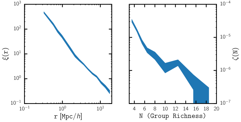
For our summary statistics of the catalogs we use: the mean number density , the galaxy two-point correlation function , and the group multiplicity function . Our mock observation catalog has and in Figure 1 we plot (left panel) and (right panel). The width of the shaded region represent the square root of the diagonal elements of the summary statistic covariance matrix, which is computed as we describe below.
We calculate using the natural estimator (Section 2.3) with fifteen radial bins. The edges of the first radial bin are and . The bin edges for the next 14 bins are logarithmically-spaced between and . We compute the as described in Section 2.3 with nine richness bins where the bin edges are logarithmically-spaced between and . To calculate the covariance matrix, we first run the forward model using the true HOD parameters for all halo catalog subvolumes: . We compute the summary statistics of each subvolume galaxy sample :
| (13) |
Then we compute the covariance matrix as
| (14) | |||||
| (15) |
Throughout our ABC-PMC analysis, we treat the , , and we describe in this section as if they were the summary statistics of actual observations. However, we benefit from the fact that these observables are generated from mock observations using the true HOD parameters of our choice: we can use the true HOD parameters to assess the quality of the parameter constraints we obtain from ABC-PMC.
3.2 ABC-PMC Design
In Section 2.1, we describe the key components of the ABC algorithm we use in our analysis. Now, we describe the more specific choices we make within the algorithm: the distance metric, the choice of priors, the distance threshold, and the convergence criteria. So far we have described three summary statistics: , , and . In order to explore the detailed differences in the ABC-PMC parameter constraints based on our choice of summary statistics, we run our analysis for two sets of observables: (, ) and (, ).
For both analyses, we use a multi-component distance (Silk et al. 2012, Cisewsky et al in preparation). Each summary statistic has a distance associated to it: , , and . We calculate each of these distance components as,
| (16) | |||||
| (17) | |||||
| (18) |
The superscripts and denote the data and model respectively. The data, are the observables calculated from the mock observation (Section 3.1). , , and are not the diagonal elements of the covariance matrix (14). Instead, they are diagonal elements of the covariance matrix .
We construct by populating the entire halo catalogs times repeatedly, calculating , , and for each realization, and then computing the covariance associated with these observables across all realizations. We highlight that differs from Eq. 14, in that it does not populate the subvolumes but the entire simulation and therefore does not incorporate sample variance. The ABC-PMC analysis instead accounts for the sample variance through the forward generative model, which populates the subvolumes in the same manner as the observations. We use , , and to ensure that the distance is not biased to variations of observables on specific radial or richness bin.
For our ABC-PMC analysis using the observables and , our distance metric while the distance metric for the ABC-PMC analysis using the observables and , is . To avoid any complications from the choice for our prior, we select uniform priors over all parameters aside from the scatter parameter , for which we choose a log-uniform prior. We list the range of our prior distributions in Table 1.
With the distances and priors specified, we now describe the distance thresholds and the convergence criteria we impose in our analyses. For the initial iteration, we set distance thresholds for each distance component to . This means, that the initial pool is simply sampled from the prior distribution we specify above. After the initial iteration, the distance threshold is adaptively lowered in subsequent iterations. More specifically, we follow the choice of Lin & Kilbinger (2015) and set the distance threshold to the median of , the multi-component distance of the previous iteration of particles ().
The distance threshold will progressively decrease. Eventually after a sufficient number of iterations, the region of parameter space occupied by will remain unchanged. As this happens, the acceptance ratio begins to fall significantly. When the acceptance ratio drops below , our acceptance ratio threshold of choice, we deem the ABC-PMC algorithm as converged. In addition to the acceptance ratio threshold we impose, we also ensure that distribution of the parameters converges – another sign that the algorithm has converged. Next, we present the results of our ABC-PMC analyses using the sets of observables (, ) and (, ).
| HOD Parameter | Prior | Range |
|---|---|---|
| Uniform | [0.8, 1.3] | |
| Log-Uniform | [0.1, 0.7] | |
| Uniform | [10.0, 13.0] | |
| Uniform | [11.02, 13.02] | |
| Uniform | [13.0, 14.0] |
3.3 Results: ABC
We describe the ABC algorithm in Section 2.1 and list the particular choices we make in the implementation in the previous section. Finally, we demonstrate how the ABC algorithm produces parameter constraints and present the results of our ABC analysis – the parameter constraints for the Zheng et al. (2007) HOD model.
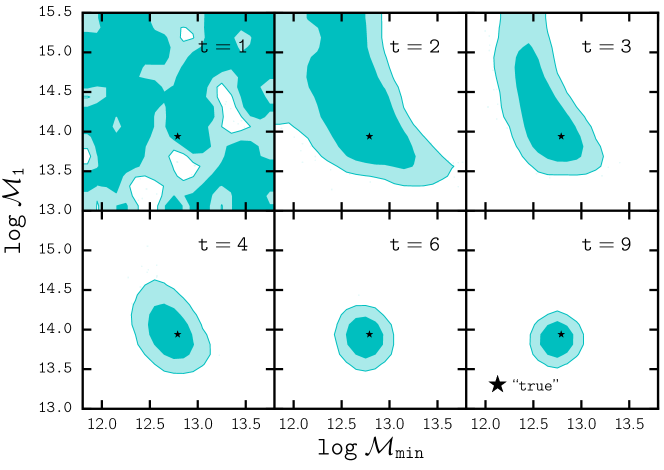
We begin with a qualitative demonstration of the ABC algorithm in Figure 2, where we plot the evolution of the ABC over the iterations to , in the parameter space of . The ABC procedure we plot in Figure 2 uses and for observables, but the overall evolution is the same when we use and . The darker and lighter contours represent the and confident regions of the posterior distribution over . For reference, we also plot the “true” HOD parameter (black star) in each of the panels. The parameter ranges of the panels are equivalent to the ranges of the prior probabilities we specify in Table 1.
For , the initial pool (top left), the distance threshold , so uniformly samples the prior probability over the parameters. At each subsequent iteration, the threshold is lowered (Section 3), so for panels, we note that the parameter spaced occupied by dramatically shrinks. Eventually when the algorithm begins to converge, , the contours enclosing the and confidence interval stabilize. At the final iteration (bottom right), the algorithm has converged and we find that lies within the confidence interval of the particle distribution. This distribution at the final iteration represents the posterior distribution of the parameters.
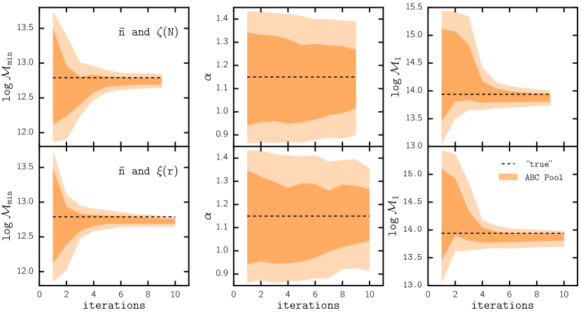
To better illustrate the criteria for convergence, in Figure 3, we plot the evolution of the distribution as a function of iteration for parameters (left), (center), and (right). The darker and lighter shaded regions correspond to the and confidence levels of the distributions. The top panels correspond to our ABC results using as observables and the bottom panels correspond to our results using . For each of the parameters in both top and bottom panels, we find that the distribution does not evolve significantly for . At this point additional iterations in our ABC algorithm will neither impact the distance threshold nor the posterior distribution of . We also emphasize that the convergence of the parameter distributions coincides with when the acceptance ratio, discussed in Section 3.2, crosses the predetermined shut-off value of . Based on these criteria, our ABC results for both and observables have converged.
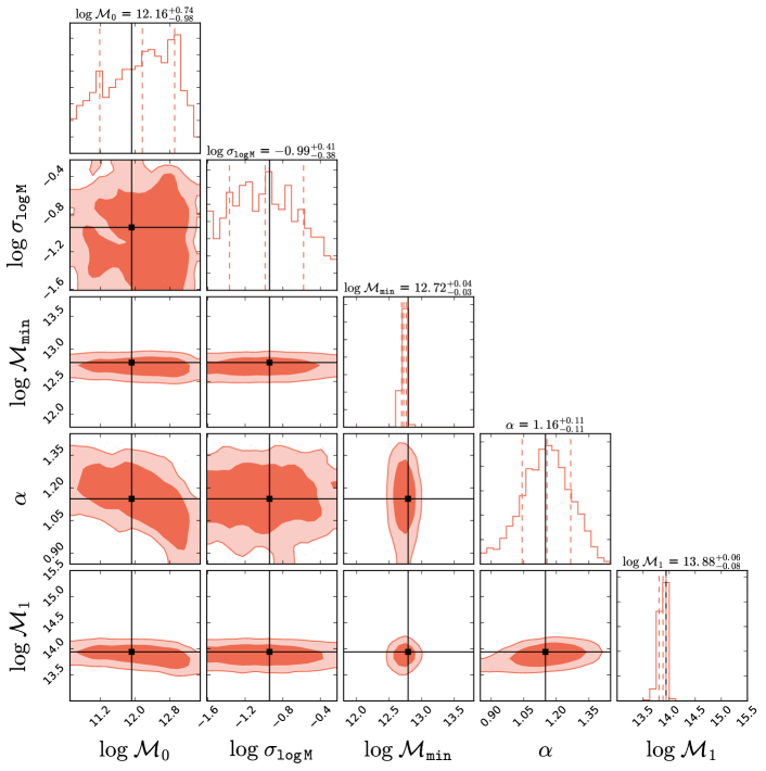
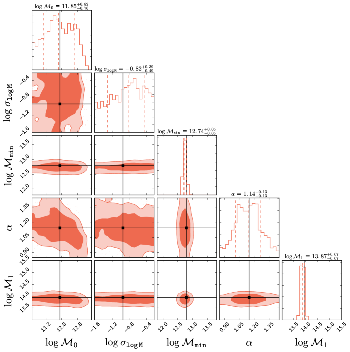
We present the parameter constraints from the converged ABC analysis in Figure 4 and Figure 5. Figure 4 shows the parameter constraints using and while Figure 5 plots the constraints using and . For both figures, the diagonal panels plot the posterior distribution of the HOD parameters with vertical dashed lines marking the (median) and confidence intervals. The off-diagonal panels plot the degeneracy between parameter pairs. To determine the accuracy of our ABC parameter constraints, we plot the “true” HOD parameters (black) in each of the panels. For both sets of observables, our ABC constraints are consistent with the “true” HOD parameters. For , , and , the true parameter values lie near the center of the confidence interval. For the other parameter, which have much tighter constraints, the true parameters lie within the confidence interval.
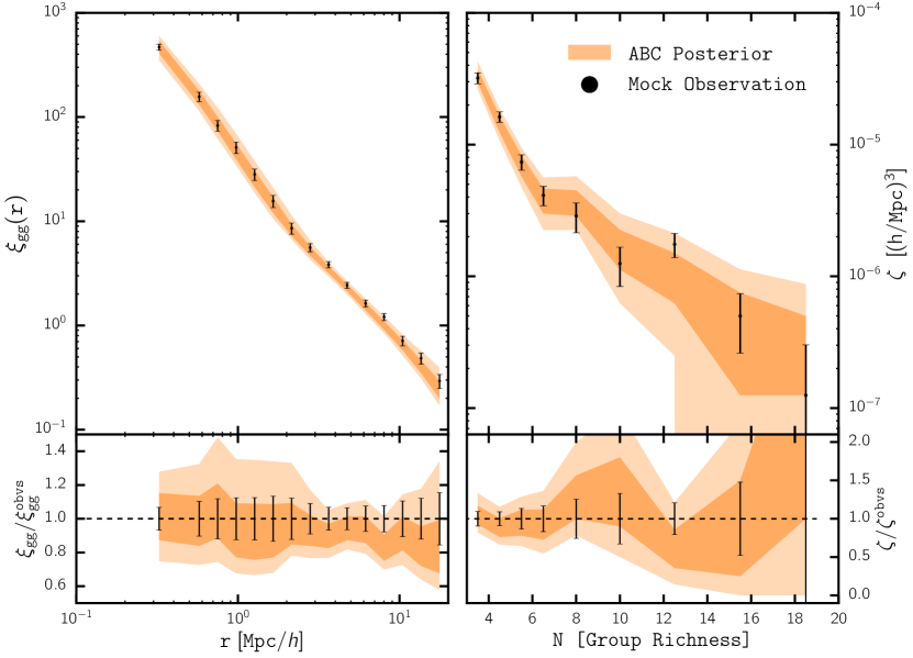
To further test the ABC results, in Figure 6, we compare (left) and (right) of the mock observations from Section 3.1 to the predictions of the ABC posterior distribution (shaded). The error bars of the mock observations represent the square root of the diagonal elements of the covariance matrix (Eq. 14) while the darker and lighter shaded regions represent the and confidence regions of the ABC posterior predictions. In the lower panels, we plot the ratio of the ABC posterior prediction and over the mock observation and . Overall, the ratio of the confidence region of ABC posterior predictions is consistent with unity throughout the and range. We observe slight deviations in the ratio for ; however, any deviation is within the uncertainties of the mock observations. Therefore, the observables drawn from the ABC posterior distributions are in good agreement with the observables of the mock observation.
The ABC results we obtain using the algorithm of Section 2.1 with the choices of Section 3.2 produce parameter constraints that are consistent with the “true” HOD parameters (Figures 4 and 5). They also produce observables and that are consistent with and . Thus, through ABC we are able to produce consistent parameter constraints. More importantly, we demonstrate that ABC is feasible for parameter inference in large scale structure.
3.4 Comparison to the Gaussian Pseudo-Likelihood MCMC Analysis
In order to assess the quality of the parameter inference described in the previous section, we compare the ABC-PMC results with the HOD parameter constraints from assuming a Gaussian likelihood function. The model used for the Gaussian likelihood analysis is different than the forward generative model adopted for the ABC-PMC algorithm, to be consistent with the standard approach.
In the ABC analysis, the model accounts for sample variance by randomly sampling a subvolume to be populated with galaxies. Instead, in the Gaussian pseudo-likelihood analysis, the covariance matrix is assumed to capture the uncertainties from sample variance. Hence, in the model for the Gaussian pseudo-likelihood analysis, we populate halos of the entire simulation rather than a subvolume. We describe the Gaussian pseudo-likelihood analysis below.
To write down the Gaussian pseudo-likelihood, we first introduce the vector : a combination of the summary statistics (observables) for a galaxy catalog. When we use and as observables in the analysis: ; when we use and as observables in the analysis: . Based on this notation, we can write pseudo-likelihood function as
| (19) |
where
| (20) |
the difference between , measured from the mock observation, and measured from the mock catalog generated from the model with parameters . here is the dimension of (for , ; for , ). is the inverse covariance matrix, which we estimate following Hartlap et al. (2007):
| (21) |
is the estimated covariance matrix, calculated using the corresponding block of the covariance matrix from Eq. 14, and is the number of mocks used for the estimation (; see Section 3.1). We note that in the dependence on the HOD parameters is neglected, so the second term in the expression of Eq. 19 can be neglected. Finally, using this pseudo-likelihood, we sample from the posterior distribution given the prior distribution using the MCMC sampler (Foreman-Mackey et al. 2013).
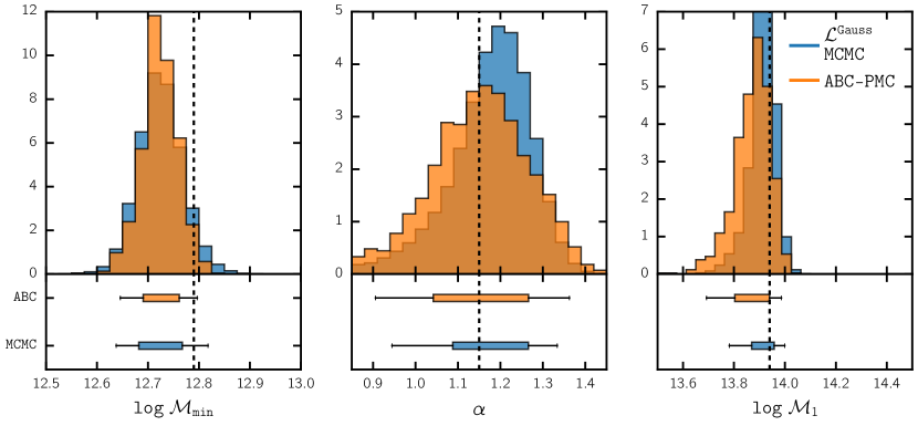
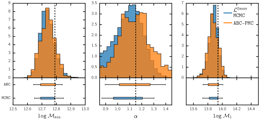
In Figures 7 and 8, we compare the results from ABC-PMC and Gaussian pseudo-likelihood MCMC analyses using and as observables, respectively. The top panels in each figure compares the marginalized posterior PDFs for three parameters of the HOD model: . The lower panels in each figure compares the and confidence intervals of the constraints derived from the two inference methods as a box plot. The “true” HOD parameters are marked by vertical dashed lines in each panel.
In both Figures 7 and 8, the marginalized posteriors for each of the parameters from both inference methods are comparable and consistent with the “true” HOD parameters. However, we note that there are minor discrepancies between the maringalized posterior distributions. In particular, the distribution for derived from ABC-PMC is less biased than the constraints from the Gaussian pseudo-likelihood approach.
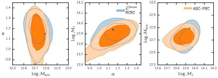
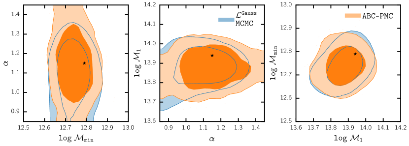
In Figures 9 and 10, we plot the contours enclosing the and confidence regions of the posterior probabilities of the two methods using and as observables respectively. In both figures, we mark the “true” HOD parameters (black star). The overall shape of the contours are in agreement with each other. However, we note that the contours for the ABC-PMC method are more extended along .
Overall, the HOD parameter constraints from ABC-PMC are consistent with those from the Gaussian pseudo-likelihood MCMC method; however, using ABC-PMC has a number of advantages. For instance, ABC-PMC utilizes a forward generative model. Our forward generative model accounts for sample variance. On the other hand, the Gaussian pseudo-likelihood approach, as mentioned earlier this section, does not account for sample variance in the model and relies on the covariance matrix estimate to capture the sample variance of the data.
Accurate estimation of the covariance matrix in LSS, however, faces a number of challenges. It is both labor and computationally expensive and dependent on the accuracy of simulated mock catalogs, known to be unreliable on small scales (see Heitmann et al. 2008; Chuang et al. 2015 and references therein). In fact, as Sellentin & Heavens (2016) points out, using estimates of the covariance matrix in the Gaussian psuedo-likelihood approach become further problematic. Even when inferring parameters from a Gaussian-distributed data set, using covariance matrix estimates rather than the true covariance matrix leads to a likelihood function that is no longer Gaussian. ABC-PMC does not depend on a covariance matrix estimate; hence, it does not face these problems.
In addition to not requiring accurate covariance matrix estimates, forward models of the ABC-PMC method, in principle, also have the advantage that they can account for sources of systematic uncertainties that affect observations. All observations suffer from significant systematic effects which are often difficult to correct. For instance, in SDSS-III BOSS (Dawson et al., 2013), fiber collisions and redshift failures siginifcantly bias measurements and analysis of observables such as or the galaxy powerspectrum (Ross et al., 2012; Guo et al., 2012; Hahn et al., 2017). In parameter inference, these systematics can affect the likelihood, and thus any analysis that requires writing down the likelihood, in unknown ways. With a forward generative model of the ABC-PMC method, the systematics can be simulated and marginalized out to achieve unbiased constraints.
Furthermore, ABC-PMC – unlike the Gaussian pseudo-likelihood approach – is agnostic about the functional form of the underlying distribution of the summary statistics (e.g. and ). As we explain throughout the paper, the likelihood function in LSS cannot be Gaussian. For , the correlation function must satisfy non-trivial positive-definiteness requirements and hence the Gaussian pseudo-likelihood function assumption is not correct in detail. In the case of , assuming a Gaussian functional form for the likelihood, which in reality is more likely Poisson, misrepresents the true likelihood function. In fact, this incorrect likelihood, may explain why the constraints on are less biased for the ABC-PMC analysis than the Gaussian-likelihood analysis in 10.
Although in our comparison using simple mock observations, we find generally consistent parameter constraints from both the ABC-PMC analysis and the standard Gaussian pseudo-likelihood analysis, more realistic scenarios present many factors that can generate inconsistencies. Consider a typical galaxy catalog from LSS observations. These catalogs consist of objects with different data qualities, signal-to-noise ratios, and systematic effects. For example, catalogs are often incomplete beyond some luminosity/redshift or have some threshold signal-to-noise ratio cut imposed on them.
These selection effects, coupled with the systematic effects earlier this section, make correctly predicting the likelihood intractable. In the standard Gaussian pseudo-likelihood analysis, and other analysis that require writing down a likelihood function, these effects can significantly bias the inferred parameter constraints. In these situations, employing ABC equipped with a generative forward model that incorproates selection and systematic effects may produce less biased parameter constraints.
Despite the advantages of ABC, one obstactle for adopting it to parameter inference has been the computational costs of generative forward models, a key element of ABC. By combining ABC with the PMC sampling method, however, ABC-PMC efficiently converges to give reliable posterior parameter constraints. In fact, in our analysis, the total computational resources required for the ABC-PMC analysis were comparable to the computational resources used for the Gaussian pseudo-likelihood analysis with MCMC sampling.
Applying ABC-PMC beyond the analysis in this work, to broader LSS analyses imposes some caveats. In this work, we focus on the galaxy-halo connection, so our generative forward model populates halos with galaxies. LSS analyses for inferring cosmological parameters would require generating halos by running cosmological simulations. The forward models also need to accurately model the observation systematic effects of the latest observations. Hence, accurate generative forward models in LSS analyses demand improvements in simulations and significant computational resources in order to infer unbiased parameter constraints. Recent cosmology simulations show promising improvements in both accuracy and speed (e.g. Feng et al., 2016). Such developements will be crucial for applying ABC-PMC to broader LSS analyses and exploiting the significant advantages that ABC-PMC offers.
4 Summary and Conclusion
Approximate Bayesian Computation, ABC, is a generative, simulation-based inference that can deliver correct parameter estimation with appropriate choices for its design. It has the advantage over the standard approach in that it does not require explicit knowledge of the likelihood function. It only relies on the ability to simulate the observed data, accounting for the uncertainties associated with observation and on specifying a metric for the distance between the observed data and simulation. When the specification of the likelihood function proves to be challenging or when the true underlying distribution of the observable is unknown, ABC provides a promising alternative for inference.
The standard approach to large scale structure studies relies on the assumption that the likelihood function for the observables – often two-point correlation function – given the model has a Gaussian functional form. In other words, it assumes that the statistical summaries are Gaussian distributed. In principle to rigorously test such an assumption, a large number of realistic simulations would need to be generated in order to examine the actual distribution of the observables. This process, however, is prohibitively—both labor and computationally —expensive. Therefore, our assumption of a Gaussian likelihood function remains largely unconfirmed and so unknown. Fortunately, the framework of ABC permits us to bypass any assumptions regarding the distribution of observables. Through ABC, we can provide constraints for our models without making the unexamined assumption of Gaussianity.
With the ultimate goal of demonstrating that ABC is feasible for LSS studies, we use it to constrain parameters of the halo occupation distribution, which dictates the galaxy-halo connection. We begin by constructing a mock observation of galaxy distribution with a chosen set of “true” HOD model parameters. Then we attempt to constrain these parameters using ABC. More specifically, in this paper:
-
•
We provide an explanation of the ABC algorithm and present how Population Monte Carlo can be utilized to efficiently reach convergence and estimate the posterior distributions of model parameters. We use this ABC-PMC algorithm with a generative forward model built with , a software package for creating catalogs of galaxy positions based on models of the galaxy-halo connection such as the HOD.
-
•
We choose , and as observables and summary statistics of the galaxy position catalogs. And for our ABC-PMC algorithm, we specify a multi-component distance metric, uniform priors, a median threshold implementation, and an acceptance rate-based convergence criterion.
-
•
From our specific ABC-PMC method, we obtain parameter constraints that are consistent with the “true” HOD parameters of our mock observations. Hence we demonstrate that ABC-PMC can be used for parameter inference in LSS studies.
-
•
We compare our ABC-PMC parameter constraints to constraints using the standard Gaussian-likelihood MCMC analysis. The constraints we get from both methods are comparable in accuracy and precision. However, for our analysis using and in particular, we obtain less biased posterior distributions when comparing to the “true” HOD parameters.
Based on our results, we conclude that ABC-PMC is able to consistently infer parameters in the context of LSS. We also find that the computation required for our ABC-PMC and standard Gaussian-likelihood analyses are comparable. Therefore, with the statistical advantages that ABC offers, we present ABC-PMC as an improved alternative for parameter inference.
Acknowledgements
We thank Jessie Cisewsky for reading and making valuable comments on the draft. We would also like to thank Michael R. Blanton, Jeremy R. Tinker, Uros Seljak, Layne Price, Boris Leidstadt, Alex Malz, Patrick McDonald, and Dan Foreman-Mackey for productive and insightful discussions. MV was supported by NSF grant AST-1517237. DWH was supported by NSF (grants IIS-1124794 and AST-1517237), NASA (grant NNX12AI50G), and the Moore-Sloan Data Science Environment at NYU. KW was supported by NSF grant AST-1211889. Computations were performed using computational resources at NYU-HPC. We thank Shenglong Wang, the administrator of NYU-HPC computational facility, for his consistent and continuous support throughout the development of this project. We would like to thank the organizers of the AstroHackWeek 2015 workshop (http://astrohackweek.org/2015/), since the direction and the scope of this investigation was —to some degree— initiated through discussions in this workshop. Throughout this investigation, we have made use of publicly available software packages and . We have also used the publicly available python implementation of the FoF algorithm (https://github.com/simongibbons/pyfof).
References
- Akeret et al. (2015) Akeret J., Refregier A., Amara A., Seehars S., Hasner C., 2015, J. Cosmology Astropart. Phys., 8, 043
- Ata et al. (2015) Ata M., Kitaura F.-S., Müller V., 2015, MNRAS, 446, 4250
- Beaumont et al. (2009) Beaumont M. A., Cornuet J.-M., Marin J.-M., Robert C. P., 2009, Biometrika, p. asp052
- Behroozi et al. (2013a) Behroozi P. S., Wechsler R. H., Wu H.-Y., 2013a, ApJ, 762, 109
- Behroozi et al. (2013b) Behroozi P. S., Wechsler R. H., Conroy C., 2013b, ApJ, 770, 57
- Berlind & Weinberg (2002) Berlind A. A., Weinberg D. H., 2002, ApJ, 575, 587
- Berlind et al. (2006) Berlind A. A., et al., 2006, ApJS, 167, 1
- Bernardeau et al. (2002) Bernardeau F., Colombi S., Gaztañaga E., Scoccimarro R., 2002, Phys. Rep., 367, 1
- Bishop (2007) Bishop C., 2007, Pattern Recognition and Machine Learning (Information Science and Statistics), 1st edn. 2006. corr. 2nd printing edn
- Bond et al. (1991) Bond J. R., Cole S., Efstathiou G., Kaiser N., 1991, ApJ, 379, 440
- Cacciato et al. (2013) Cacciato M., van den Bosch F. C., More S., Mo H., Yang X., 2013, MNRAS, 430, 767
- Cameron & Pettitt (2012) Cameron E., Pettitt A. N., 2012, MNRAS, 425, 44
- Casas-Miranda et al. (2002) Casas-Miranda R., Mo H. J., Sheth R. K., Boerner G., 2002, MNRAS, 333, 730
- Chuang et al. (2015) Chuang C.-H., et al., 2015, MNRAS, 452, 686
- Conroy & Wechsler (2009) Conroy C., Wechsler R. H., 2009, ApJ, 696, 620
- Cooray & Sheth (2002) Cooray A., Sheth R., 2002, Phys. Rep., 372, 1
- Davis et al. (1985) Davis M., Efstathiou G., Frenk C. S., White S. D. M., 1985, ApJ, 292, 371
- Dawson et al. (2013) Dawson K. S., et al., 2013, AJ, 145, 10
- Del Moral et al. (2006) Del Moral P., Doucet A., Jasra A., 2006, Journal of the Royal Statistical Society: Series B (Statistical Methodology), 68, 411
- Dressler (1980) Dressler A., 1980, ApJ, 236, 351
- Dutton & Macciò (2014) Dutton A. A., Macciò A. V., 2014, MNRAS, 441, 3359
- Eriksen et al. (2004) Eriksen H. K., et al., 2004, ApJS, 155, 227
- Feng et al. (2016) Feng Y., Chu M.-Y., Seljak U., 2016, preprint, (arXiv:1603.00476)
- Filippi et al. (2011) Filippi S., Barnes C., Stumpf M., 2011, arXiv preprint arXiv:1106.6280
- Foreman-Mackey et al. (2013) Foreman-Mackey D., Hogg D. W., Lang D., Goodman J., 2013, PASP, 125, 306
- Guo et al. (2012) Guo H., Zehavi I., Zheng Z., 2012, ApJ, 756, 127
- Hahn et al. (2017) Hahn C., Scoccimarro R., Blanton M. R., Tinker J. L., Rodríguez-Torres S., 2017, MNRAS,
- Hartlap et al. (2007) Hartlap J., Simon P., Schneider P., 2007, A&A, 464, 399
- Hearin et al. (2016a) Hearin A., et al., 2016a, preprint, (arXiv:1606.04106)
- Hearin et al. (2016b) Hearin A. P., Zentner A. R., van den Bosch F. C., Campbell D., Tollerud E., 2016b, MNRAS,
- Heitmann et al. (2008) Heitmann K., et al., 2008, Computational Science and Discovery, 1, 015003
- Heitmann et al. (2009) Heitmann K., Higdon D., White M., Habib S., Williams B. J., Lawrence E., Wagner C., 2009, ApJ, 705, 156
- Heitmann et al. (2010) Heitmann K., White M., Wagner C., Habib S., Higdon D., 2010, ApJ, 715, 104
- Ishida et al. (2015) Ishida E. E. O., Vitenti S. D. P., Penna-Lima M., Cisewski J., de Souza R. S., Trindade A. M. M., Cameron E., Busti V. C., 2015, Astronomy and Computing, 13, 1
- Kaiser (1984) Kaiser N., 1984, ApJ, 284, L9
- Klypin et al. (2011) Klypin A. A., Trujillo-Gomez S., Primack J., 2011, ApJ, 740, 102
- Knox (1995) Knox L., 1995, Phys. Rev. D, 52, 4307
- Kravtsov et al. (1997) Kravtsov A. V., Klypin A. A., Khokhlov A. M., 1997, ApJS, 111, 73
- Leach et al. (2008) Leach S. M., et al., 2008, A&A, 491, 597
- Leauthaud et al. (2012) Leauthaud A., et al., 2012, ApJ, 744, 159
- Lemson & Kauffmann (1999) Lemson G., Kauffmann G., 1999, MNRAS, 302, 111
- Lin & Kilbinger (2015) Lin C.-A., Kilbinger M., 2015, A&A, 583, A70
- Lin et al. (2016) Lin C.-A., Kilbinger M., Pires S., 2016, preprint, (arXiv:1603.06773)
- Miyatake et al. (2015) Miyatake H., et al., 2015, ApJ, 806, 1
- Mo & White (1996) Mo H. J., White S. D. M., 1996, MNRAS, 282, 347
- More et al. (2009) More S., van den Bosch F. C., Cacciato M., 2009, MNRAS, 392, 917
- More et al. (2013) More S., van den Bosch F. C., Cacciato M., More A., Mo H., Yang X., 2013, MNRAS, 430, 747
- Navarro et al. (2004) Navarro J. F., et al., 2004, MNRAS, 349, 1039
- Oh et al. (1999) Oh S. P., Spergel D. N., Hinshaw G., 1999, ApJ, 510, 551
- Peebles (1980) Peebles P. J. E., 1980, The large-scale structure of the universe
- Planck Collaboration et al. (2014) Planck Collaboration et al., 2014, A&A, 571, A16
- Planck Collaboration et al. (2015a) Planck Collaboration et al., 2015a, preprint, (arXiv:1502.01589)
- Planck Collaboration et al. (2015b) Planck Collaboration et al., 2015b, preprint, (arXiv:1502.01592)
- Planck Collaboration et al. (2015c) Planck Collaboration et al., 2015c, preprint, (arXiv:1502.02114)
- Press & Schechter (1974) Press W. H., Schechter P., 1974, ApJ, 187, 425
- Pritchard et al. (1999) Pritchard J. K., Seielstad M. T., Perez-Lezaun A., Feldman M. W., 1999, Molecular biology and evolution, 16, 1791
- Riebe et al. (2011) Riebe K., et al., 2011, preprint, (arXiv:1109.0003)
- Riess et al. (1998) Riess A. G., et al., 1998, AJ, 116, 1009
- Rodríguez-Torres et al. (2015) Rodríguez-Torres S. A., et al., 2015, preprint, (arXiv:1509.06404)
- Ross et al. (2012) Ross A. J., et al., 2012, MNRAS, 424, 564
- Santiago & Strauss (1992) Santiago B. X., Strauss M. A., 1992, ApJ, 387, 9
- Scoccimarro et al. (2001) Scoccimarro R., Sheth R. K., Hui L., Jain B., 2001, ApJ, 546, 20
- Seljak (2000) Seljak U., 2000, MNRAS, 318, 203
- Sellentin & Heavens (2016) Sellentin E., Heavens A. F., 2016, MNRAS, 456, L132
- Silk et al. (2012) Silk D., Filippi S., Stumpf M. P. H., 2012, preprint, (arXiv:1210.3296)
- Somerville & Davé (2015) Somerville R. S., Davé R., 2015, ARA&A, 53, 51
- Somerville et al. (2001) Somerville R. S., Lemson G., Sigad Y., Dekel A., Kauffmann G., White S. D. M., 2001, MNRAS, 320, 289
- Steidel et al. (1998) Steidel C. C., Adelberger K. L., Dickinson M., Giavalisco M., Pettini M., Kellogg M., 1998, ApJ, 492, 428
- Tinker et al. (2005) Tinker J. L., Weinberg D. H., Zheng Z., Zehavi I., 2005, ApJ, 631, 41
- Tinker et al. (2011) Tinker J., Wetzel A., Conroy C., 2011, preprint, (arXiv:1107.5046)
- Tinker et al. (2013) Tinker J. L., Leauthaud A., Bundy K., George M. R., Behroozi P., Massey R., Rhodes J., Wechsler R. H., 2013, ApJ, 778, 93
- Wandelt et al. (2004) Wandelt B. D., Larson D. L., Lakshminarayanan A., 2004, Phys. Rev. D, 70, 083511
- Weyant et al. (2013) Weyant A., Schafer C., Wood-Vasey W. M., 2013, ApJ, 764, 116
- White & Scott (1996) White M., Scott D., 1996, Comments on Astrophysics, 18
- Zheng et al. (2005) Zheng Z., et al., 2005, ApJ, 633, 791
- Zheng et al. (2007) Zheng Z., Coil A. L., Zehavi I., 2007, ApJ, 667, 760
- van den Bosch et al. (2003) van den Bosch F. C., Mo H. J., Yang X., 2003, MNRAS, 345, 923
- van den Bosch et al. (2013) van den Bosch F. C., More S., Cacciato M., Mo H., Yang X., 2013, MNRAS, 430, 725