The Molecular Clouds Fueling a 1/5 Solar Metallicity Starburst

Abstract

Using the Atacama Large Millimeter/submillimeter Array, we have made the first high spatial and spectral resolution observations of the molecular gas and dust in the prototypical blue compact dwarf galaxy . The $\rm{{}^{12}CO({2}-{1})}$ and $\rm{{}^{12}CO({3}-{2})}$ emission is clumpy and distributed throughout the central star-forming region. Only one of eight molecular clouds has associated star formation. The continuum spectral energy distribution is dominated by free-free and synchrotron; at 870µm, only 50% of the emission is from dust. We derive a CO-to-H₂ conversion factor using several methods, including a new method that uses simple photodissocation models and resolved CO line intensity measurements to derive a relationship that uniquely predicts $\alpha_{co}$ for a given metallicity. We find that the CO-to-H₂ conversion factor is 4 to 35 times that of the Milky Way (18.1 to 150.5  $\rm M_{\odot}(\rm K\,\rm{km\,s}^{-1}\,pc^{2})^{-1}$). The star formation efficiency of the molecular gas is at least 10 times higher than that found in normal spiral galaxies, which is likely due to the burst-dominated star formation history of  rather than an intrinsically higher efficiency. The molecular clouds within  resemble those in other strongly interacting systems like the Antennae: overall they have high size-linewidth coefficients and molecular gas surface densities. These properties appear to be due to the high molecular gas surface densities produced in this merging system rather than to increased external pressure. Overall, these results paint a picture of  as a complex, rapidly evolving system whose molecular gas properties are dominated by the large-scale gas shocks from its on-going merger.

I. Introduction

The high star formation rate surface densities and low metallicities found in blue compact dwarf galaxies represent one of the most extreme environments for star formation in the local universe, one more akin to that found in high redshift galaxies than in local spirals (Cardamone et al., 2009; Izotov et al., 2011). These global properties result in increased disruption of the interstellar medium by newly formed young massive stars (Krumholz et al., 2006; Murray et al., 2010), higher and harder radiation fields (Madden et al., 2006), and reduced dust content (Rémy-Ruyer et al., 2013), all of which may significantly change how the molecular gas within these galaxies transforms into stars. To date, however, the molecular gas fueling the starbursts within blue compact dwarfs remains poorly understood due to the intrinsically faint emission from the most common molecular gas tracers (CO and dust continuum). By quantifying the properties of molecular gas in blue compact dwarfs, we can determine how the physical conditions in these galaxies influence their molecular gas, and thus the formation of young massive stars, as well as gain insight into star formation in high redshift galaxies, where detailed observations are difficult.

Previous low-resolution studies of molecular gas in low-metallicity galaxies, including blue compact dwarfs, have shown that these galaxies have extremely high star formation rates compared to their CO luminosity – a key tracer of the bulk molecular gas – and that this ratio increases as the metallicity of a galaxy decreases (Taylor et al., 1998; Schruba et al., 2012). Taken by itself, this trend suggests that low-metallicity galaxies either have increased molecular star formation efficiency (i.e., less molecular gas is necessary to form a given amount of stars) or that CO emission is not as effective as tracer of molecular gas because of the decreased dust shielding and reduced abundance of molecules in low metallicity environments (i.e., less CO emission for a given amount of molecular gas). Distinguishing between these two scenarios, however, requires higher spatial resolution to directly measure the CO-to-H₂ conversion factor (and thus determine the total molecular gas mass) and to link the young massive stars within the galaxy to the giant molecular clouds from which they presumably form (although see Krumholz, 2012 and Glover & Clark, 2012 for arguments that neutral hydrogen may play an increasing role in star-forming clouds at low metallicity).

Resolved giant molecular cloud observations in low-metallicity galaxies have historically been very difficult because of the faint nature of the CO emission in these systems. One of the few resolved studies of giant molecular clouds in a sample of dwarf galaxies showed that the giant molecular clouds in these galaxies have similar sizes, linewidths, and CO-to-H₂ conversion factors to more massive spiral galaxies like the Milky Way, M33, and M31, which supports the idea of higher star formation efficiencies (Bolatto et al., 2008). In contrast, estimates of the CO-to-H₂ conversion factor from resolved dust observations find systematically higher values for low-metallicity galaxies, suggesting that dwarf galaxies have lower CO luminosities for a given amount of molecular gas (Leroy et al., 2011). These two apparently contradictory sets of observations can be reconciled if the reduced dust shielding for CO in low metallicity environments pushes the CO emission to the densest portion of the molecular cloud, while the H₂ remains distributed throughout the molecular cloud because it can self-shield. Therefore, the CO observations only trace the central regions of the molecular clouds, while the infrared observations trace the dust, which is well-mixed with the surrounding envelope of molecular gas (Bolatto et al., 2008; Leroy et al., 2011; Sandstrom et al., 2013).

The sensitivity of the previous generation of millimeter interferometers limited the sample in the most comprehensive study to date (Bolatto et al., 2008) to nearby galaxies ($\lesssim 4$ Mpc) with relatively high metallicities; only one galaxy has a metallicity less than 12+log(O/H)=8.2. Therefore, it is not surprising that these authors see little variation in the sizes, linewidths, and CO-to-H₂ conversion factors of low metallicity galaxies. Intriguingly, they do see hints that the lowest metallicity galaxy included in their sample (the Small Magellanic Cloud) may deviate from the fiducial trends seen in normal galaxies, although the deviations are relatively weak. This result suggests that expanding resolved molecular gas studies to lower metallicities and more extreme systems than possible with the previous generation of millimeter interferometers may uncover more variations in molecular cloud properties. Fortunately, today we have access to the Atacama Large Millimeter/submillimeter Array (ALMA), whose excellent sensitivity and resolution allow us to do just this.

The blue compact dwarf galaxy  represents a key test case for understanding how the properties of molecular clouds vary with metallicity and star formation rate surface density: this galaxy bridges the gap between ultra-low metallicity ($\sim 1/50Z_{\odot}$) starburst galaxies like SBS 0335-052 and I Zw 18 and starbursting galaxies with normal solar metallicities. Although  has only a moderate metallicity (12+log(O/H)=8.09; Guseva et al., 2000), roughly comparable to the SMC, its central star-forming region has an extraordinarily high star formation rate surface density of 520 $\rm{M}_{\odot}\,{\rm yr^{-1}\,kpc^{-2}}$ (Kepley et al., 2014), comparable to that found in more massive starburst galaxies. Crucially for our purposes, this galaxy is also only 10 Mpc away (Tully & Fisher, 1988), which is two to five times closer than other comparable galaxies like I Zw 18 and SBS0335-052. At this distance, we can resolve the giant molecular cloud fueling the starburst within  using only moderate angular resolution – 0.5″ corresponds to 24 pc linear resolution – allowing us to quantify the resolved properties of its molecular gas. By comparing these properties to those in other starburst galaxies of varying metallicity, we can begin to disentangle the relative effects of metallicity and high star formation rate surface density on the star formation efficiencies and CO luminosities in blue compact dwarf galaxies.

In this paper, we present new, high spatial and spectral resolution ALMA observations of the molecular gas and dust content of . Our goal is to understand how the interplay of intense star formation and low metallicity within this galaxy shapes its molecular gas and dust, and whether dust and molecular gas in this galaxy differs in key ways from that in other metal-rich star-forming galaxies. To do this, we measure the properties of the dust and giant molecular clouds within . We use these measurements to derive the CO-to-H₂ conversion factor ($\alpha_{co}$) – which underlies most of what we know about star formation beyond the Local Group – in  and compare it to other observational and theoretical estimates for this factor. Then we compare the molecular cloud properties in  to the cloud properties in other systems to see if there are systematic differences in cloud properties with metallicity and/or star formation rate surface density. Finally, we use these observations to place the properties of the molecular gas and star formation within  in the larger context of star formation within galaxies.

II. Data

This paper presents ALMA Cycle 1 (proposal 2012.1.00984.S; PI: A. Kepley) observations of the CO and continuum emission from the central starburst region of the prototypical blue compact dwarf galaxy  at 3, 1 mm, and 870µm. We describe the data calibration and imaging below. Tables 1 and 2 summarize the observations and spectral window configurations.

Table 1Observation Summary

	3 mm	1 mm	870µm
Date	2014 August 30	2014 June 14	2013 Oct 09
Number of Antennas	35	33	19
Mean Wind Speed ($\rm{m\,s}^{-1}$)	9	7	6
Mean Precipitable Water Vapor (mm)	3.38	0.51	0.42
Flux Calibrator	J0510+180	J0510+180	J0510+180
Bandpass Calibrator	J0532+0732	J0607-0834	J0423-0120
Phase Calibrator	J0607-0834	J0552+0313	J0552+0313

Table 2Spectral Window Setup

	Central Sky Frequency		Rest Frequency	Bandwidth	Bandwidth	Channel Width
Band	GHz	Line	GHz	MHz	$\rm{km\,s}^{-1}$	MHz	$\rm{km\,s}^{-1}$
3 mm	114.968	$\rm{{}^{12}CO({1}-{0})}$	115.27120	468.75	1220	0.1221	0.32
	112.712	Continuum	$\cdots$	2000.0	$\cdots$	15.625	$\cdots$
	102.420	Continuum	$\cdots$	2000.0	$\cdots$	15.625	$\cdots$
	100.535	Continuum	$\cdots$	2000.0	$\cdots$	15.625	$\cdots$
1 mm	230.110	$\rm{{}^{12}CO({2}-{1})}$	230.53800	468.75	611	0.1221	0.16
	219.598	$\rm{{}^{13}CO({2}-{1})}$	220.39868	468.75	640	0.1221	0.17
	233.370	Continuum	$\cdots$	2000.0	$\cdots$	15.625	$\cdots$
	215.902	Continuum	$\cdots$	2000.0	$\cdots$	15.625	$\cdots$
870 µm	344.262	$\rm{{}^{12}CO({2}-{1})}$	345.79599	1875.0	1634	0.488281	0.43
	330.261	$\rm{{}^{13}CO({2}-{1})}$	330.58797	1875.0	1703	0.488281	0.44
	342.270	Continuum	$\cdots$	2000.0	$\cdots$	15.625	$\cdots$
	332.145	Continuum	$\cdots$	2000.0	$\cdots$	15.625	$\cdots$

The 870µm and 1 mm data were calibrated in CASA (McMullin et al., 2007) using scripts provided by the North American ALMA Science Center (NAASC). First, the water vapor radiometer corrections and system temperatures were calculated and applied to the data, and the flux density of the flux calibrator was set. Then the bandpass solutions were calculated using the bandpass calibrator. Next the amplitudes and phases of the calibration sources were derived. The calibration sources had per-integration phases and per-scan amplitudes derived and applied and were flux-scaled. The selected 870µm phase calibrator was faint ($\sim$ 0.06 Jy), so we combined all four spectral windows and both polarizations to increase the signal-to-noise of the solutions for that band. Finally, we applied the per-scan phases, per-scan amplitudes, and fluxscale for the phase calibrator to the science target. The 3 mm data were calibrated using the CASA pipeline version Cycle2-R1-B, which follows a similar calibration procedure.

All of the observations used quasars instead of planets to calibrate the flux density scales, which introduces additional uncertainty into the flux density scale. For the 870µm observations, the flux of the “flux” calibrator (J0510+180) decreased by 30% between the two flux measurements bracketing our observations: its measured flux density was $1.090\pm 0.06$ Jy on 2013 September 29, but had dropped to $0.710\pm 0.04$ Jy by 2013 October 20 according to the ALMA Quasar Catalogue (Fomalont et al., 2014). Extrapolating between these two values gives a flux density for J0510+180 of 0.75 Jy. We used our bandpass calibrator (J0421-120), which had a more stable flux density value, to check the accuracy of our flux density scale. Adopting the extrapolated flux density for J0510+180 yields a flux density within 5% of its measured flux. For the 1 mm observations, the flux of J0510+180 at 1 mm was measured 15 days after the observations to be 1.5 Jy. We used this measurement to set our flux density scale. Unfortunately, the bandpass and phase calibrators did not have recently measured flux densities, so we could not use them to cross-check our flux density scale. At 3 mm, the flux calibrator J0510+180 was observed within two days of our observations and had a flux of 1.56 Jy. We conservatively assume that the flux density of our observations is accurate to within 10% for the 870µm data and within 20% for the 3 mm and 1 mm data.

The data were not self-calibrated because the line and continuum emission from the source was too faint. Self-calibration typically requires a signal-to-noise of approximately 10 on an individual baseline for times on the order of a few integrations. For both data sets, the signal-to-noise on timescales of a few integrations was less than 4 for the line and continuum data.

We imaged the data in CASA. Since we are interested in measuring and comparing the CO cloud properties, we imaged the line data sets with robust = 0 to maximize angular resolution while retaining some sensitivity to larger-scale emission. The line images were restricted to the overlapping region of uv-space between the two data sets and smoothed to the same beam size to ensure that we are comparing emission on the same size scales for both lines. We also created a naturally weighted $\rm{{}^{12}CO({2}-{1})}$ image without any uv restrictions, which will be the most sensitive to emission on large angular scales, to compare to previous single-dish observations by Albrecht et al. (2004). In addition to ¹²CO, there were several additional isotopologues of CO in this data set (see Table 2). We note that the spectral window intended for $\rm{{}^{13}CO({2}-{1})}$ missed the line and thus we did not produce a $\rm{{}^{13}CO({2}-{1})}$ image.

We also created a set of continuum images from both the ALMA data presented in this paper and the VLA data from Kepley et al. (2014). We optimized for flux recovery and matching uv distributions over resolution because the three different continuum emission components – synchrotron, free-free, and dust – will have different extents. We imposed a inner uv plane limit of 16$k\lambda$ to match the largest angular scale and tapered the naturally weighted data to a $1\arcsec$ resolution and restored the data with a common 1″ beam. This procedure provided the most accurate match to the uv coverage and resolution between the relatively heterogenous uv sampling at the different wavelengths, although it is lower resolution than our line data cubes. For the VLA data, the fluxes in these images are within 10% of the fluxes measured in Kepley et al. (2014): -7% for the 4.86GHz image, -6% for the 8.45 GHz image, and 1.5% for the 22.46GHz image. Based on the single-dish continuum measurements of Klein et al. (1991), we only recover $\sim$50% of the emission from this galaxy and thus are resolving out continuum emission on larger angular scales than we probe here (12.4″). See the analysis in §4.1 of Kepley et al. (2014) for a detailed discussion of this point.

Tables 3 and 4 give a summary of our image properties. The largest angular scale of these images is approximately 12.4″.

Table 3Line Image Properties

	Rest Frequency	FOV	u-v range		Beam	PA	Velocity Resolution	Noise
Transition	GHz	″	k$\lambda$	Weighting	″	°	$\rm{km\,s}^{-1}$	$\rm{mJy\ beam^{-1}}\$	K
$\rm{{}^{12}CO({3}-{2})}$	345.79599	18.2	16.6 - 496	robust = 0	$0.54\times 0.49$	28	2 $\rm{km\,s}^{-1}$	2.6	0.1
$\rm{{}^{12}CO({2}-{1})}$	230.53800	27.3	16.6 - 496	robust = 0	$0.54\times 0.49$	28	2 $\rm{km\,s}^{-1}$	3.74	0.3
$\rm{{}^{12}CO({1}-{0})}$	115.27120	54.7	16.6 - 496	robust = 0	$0.54\times 0.49$	28	2 $\rm{km\,s}^{-1}$	5.2	1.8
$\rm{{}^{13}CO({3}-{2})}$	330.58797	19.1	16.6 - 496	robust = 0	$0.54\times 0.49$	27	2$\rm{km\,s}^{-1}$	2.4	0.1

Table 4Continuum Image Properties

Wavelength	Frequency		FOV	Beam	PA	Noise
mm	GHz	Telescope	′	″	°	$\rm{\mu Jy\ beam^{-1}}\$	mK
0.86	344.9	ALMA	0.3	$1.0\times 1.0$	0	54.2	0.55
1.3	233.3	ALMA	0.45	$1.0\times 1.0$	0	63.1	1.4
2.7	112.7	ALMA	0.93	$1.0\times 1.0$	0	41.7	4.0
13	22.46	VLA	2.0	$1.0\times 1.0$	0	53.8	130.1
35	8.46	VLA	5.3	$1.0\times 1.0$	0	58.3	993.8
62	4.86	VLA	9.3	$1.0\times 1.0$	0	16.7	862.6

III. Results

III.1. Overview of the Data

The blue compact dwarf galaxy  consists of a central starburst region, visible as a compact ($\sim$8″ = 390pc) knot in the optical, embedded within an large neutral hydrogen envelope characterized by extended tidal tails (Figure 1). Given its morphology, the starburst is the likely result of a major merger between two dwarf galaxies (Baldwin et al., 1982; van Zee et al., 1998). The burst hosts at least three young massive clusters brighter than 30 Doradus (Kepley et al., 2014), but little is known about the molecular gas that is presumably fueling this extraordinary episode of star formation.

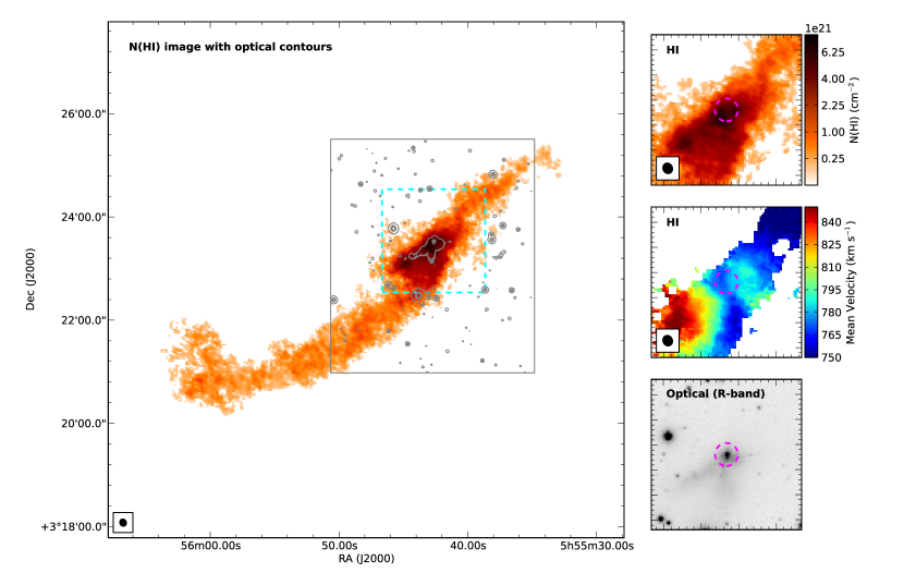
Figure 1.— The central starburst in  was likely triggered by a major merger between two dwarf galaxies as evidenced by its extended neutral hydrogen tails and compact optical emission. Left: Neutral hydrogen column density image (van Zee et al., 1998) with contours showing the R-band optical emission with the gray box showing the region observed in the optical (Gil de Paz et al., 2003). The tidal tails are seen in both neutral hydrogen and in the R-band optical image, although the neutral hydrogen tidal tails extend several times further than those seen in the optical. Right: A closer look at the neutral hydrogen and optical emission in the region outlined by the cyan box in the left panel. The right panels show (top to bottom) the neutral hydrogen column density, the neutral hydrogen mean velocity, and an optical R-band image. The field of view for the 870µm ALMA observations presented in this paper is shown as a magenta circle. These observations probe a region of relatively high HI column density ($5\times 10^{21}\,{\rm cm}^{-2}$) and a region where the HI velocity field undergoes a reversal. The optical nucleus is compact, as one would expect from an evolved merger remnant. The beam for the neutral hydrogen observations is shown in the lower left-hand corner of the relevant panels.

To quantify the properties of the molecular gas fueling the central starburst within , we used ALMA to observe $\rm{{}^{12}CO({1}-{0})}$, $\rm{{}^{12}CO({2}-{1})}$, and $\rm{{}^{12}CO({3}-{2})}$ as well as the continuum at 3 mm, 1 mm, and 870µm in a single field centered on the central starburst region, indicated by a magenta circle in the rightmost panels of Figure 1. Using high-resolution radio continuum observations, the star formation rate surface density in this region was found to be 520 $\rm{M}_{\odot}\,{\rm yr^{-1}\,kpc^{-2}}$ (Kepley et al., 2014): five orders of magnitude higher that of the solar neighborhood Milky Way value (0.003 $\rm{M}_{\odot}\,{\rm yr^{-1}\,kpc^{-2}}$) and the same order of magnitude as star formation rates in more massive starburst systems like LIRGs and ULIRGs (100-1000 $\rm{M}_{\odot}\,{\rm yr^{-1}\,kpc^{-2}}$; Kennicutt, 1998). This region also has high H I surface densities ($5\times 10^{21}{\rm cm}^{-2}$) consistent with the threshold for ${\rm H_{2}}$ formation in low metallicity galaxies (McKee & Krumholz, 2010; Wong et al., 2013) and is located near an H I velocity reversal (see the middle panel on the right-hand side of Figure 1).

Our observations detected $\rm{{}^{12}CO({2}-{1})}$ and $\rm{{}^{12}CO({3}-{2})}$ emission from the central region as well as continuum emission at all three wavelengths. We also have a global detection of $\rm{{}^{13}CO({3}-{2})}$ when we average over the main ridge of CO emission (Figure 2). The $\rm{{}^{12}CO({2}-{1})}$ emission generally has a higher brightness temperature than the $\rm{{}^{12}CO({3}-{2})}$ emission, but the $\rm{{}^{12}CO({3}-{2})}$ observations have better brightness temperature sensitivity ($\sigma_{T_{B}}\propto\sigma_{S_{\nu}}/\nu^{2}$), leading to higher signal-to-noise for the $\rm{{}^{12}CO({3}-{2})}$ data (Figure 4). The $\rm{{}^{12}CO({1}-{0})}$ line was not detected. However, given the higher noise in the $\rm{{}^{12}CO({1}-{0})}$ image (in K), this non-detection is consistent with the ratio between the $\rm{{}^{12}CO({2}-{1})}$ and $\rm{{}^{12}CO({1}-{0})}$ emission seen in  in other lower-resolution observations (0.5; Albrecht et al., 2004).

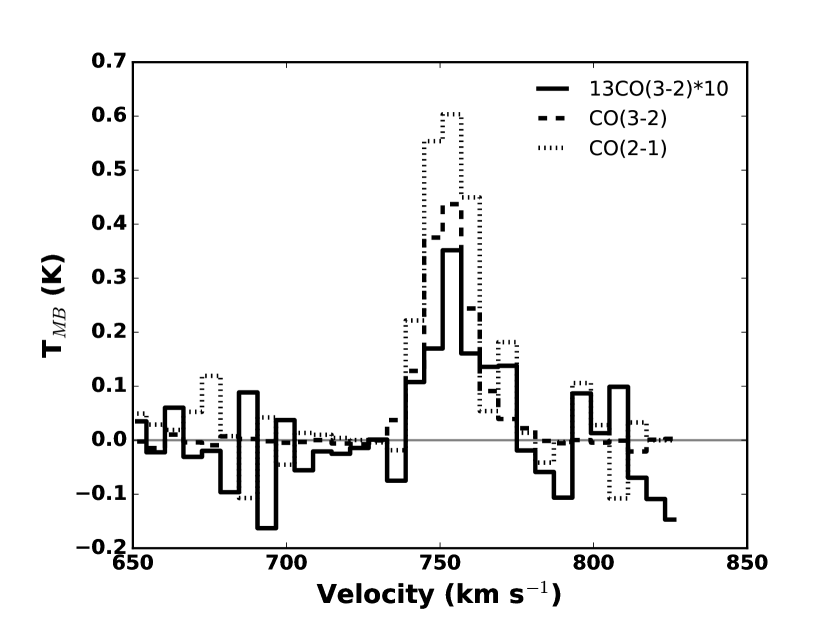
Figure 2.— Average $\rm{{}^{12}CO({3}-{2})}$, $\rm{{}^{12}CO({2}-{1})}$, and $\rm{{}^{13}CO({3}-{2})}$ spectra over the main CO ridge (extraction region corresponds to the region labeled BCD in Figure 4). We clearly detect $\rm{{}^{13}CO({3}-{2})}$ emission in the average spectrum, but do not detect it in the individual channel maps.

III.1.1 CO emission in

The observed $\rm{{}^{12}CO({2}-{1})}$ and $\rm{{}^{12}CO({3}-{2})}$ emission is clumpy and distributed throughout the central star-forming region of  (Figure 3). This CO distribution can be compared to distribution of young massive clusters traced by the 1.3 cm radio continuum emission from Kepley et al. (2014). These deep, high-resolution observations detect clusters with masses as low as $1.5\times 10^{4}\,\rm{M}_{\odot}$ anywhere within the $\rm{{}^{12}CO({3}-{2})}$ field of view. We find that only the western end of the main CO ridge is coincident with 1.3 cm continuum emission indicating recent star formation. The other 70% of the CO emission has no coincident 1.3 cm emission.

The morphology of the molecular gas emission in  strongly resembles that found in the nearby dwarf starburst galaxy NGC 1569 (Taylor et al., 1999), which is at a distance of 3.36 Mpc (Grocholski et al., 2008). In that galaxy, there are several well-separated molecular gas clouds. The molecular gas is not spatially associated with the two older ($>7$Myr) super star clusters found in the center of NGC 1569 (Hunter et al., 2000). However, the tip of one cloud is associated with an H ii region. This molecular gas distribution is in contrast to that found in observations with similar resolution of more massive (and metal-rich) starburst galaxies such as M82 (Keto et al., 2005) and the Antennae (Wei et al., 2012). In these galaxies, the molecular gas emission is much more extensive and complex, although in the case of M82 this may be more a result of the high inclination of this galaxy rather than the intrinsic molecular gas distribution. Separation of the molecular gas into individual molecular clouds for both the Antennae and M82 is much more difficult, and individually identified clouds frequently show signs of having multiple components along the line of sight (Keto et al., 2005; Wei et al., 2012). In both galaxies, the star formation appears to be concentrated on the edges of the molecular gas clouds (Keto et al., 2005; Wei et al., 2012).

The absence of 1.3 cm continuum emission from most of the CO clouds is unlikely to be the effect of extinction. Once emitted the 1.3 cm emission is unaffected by dust. We note, however, that dust can still absorb photons before they ionize the surrounding gas and produce free-free emission. This effect is roughly on the order of 30% for the Large Magellanic Cloud (Inoue, 2001) and decreases as a function of metallicity. It is also unlikely to be star formation below the 1.3 cm detection limit. The least massive CO cloud in our sample (Cloud E in Figure 12) has a mass of $\sim 2\times 10^{5}\,\rm{M}_{\odot}$, assuming the minimum $\alpha_{co}$ derived for  (see § III.2.2 for details). For a typical star formation efficiency of 3% (Heiderman et al., 2010), this implies a stellar mass of $\sim 0.5\times 10^{4}\,\rm{M}_{\odot}$ which is at the 1.3 cm detection limit. Higher $\alpha_{co}$ values for , which are likely, would imply even larger cluster masses. All this evidence suggests that the current star formation within  is associated only with the western edge of the main CO ridge and that the rest of the molecular gas does not appear to be forming stars.

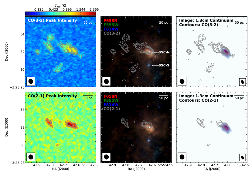
Figure 3.— The $\rm{{}^{12}CO({3}-{2})}$ and $\rm{{}^{12}CO({2}-{1})}$ emission detected by ALMA is clumpy and distributed throughout the central starburst region. Only 30% of the CO emission is coincident with star formation. Left Column: Peak intensity maps (in units of $T_{MB}$) for $\rm{{}^{12}CO({3}-{2})}$ (top) and $\rm{{}^{12}CO({2}-{1})}$ (bottom). Both images have the same resolution and are on the same color scale. The $\rm{{}^{12}CO({3}-{2})}$ contours start at 0.31 K and increase by factors of 1.3 and the $\rm{{}^{12}CO({2}-{1})}$ contours start at 1.16 K and increase by factors of $\sqrt{2}$. These images show that the $\rm{{}^{12}CO({2}-{1})}$ emission has a higher brightness temperature than the $\rm{{}^{12}CO({3}-{2})}$ emission, but the $\rm{{}^{12}CO({3}-{2})}$ data has less noise, giving the $\rm{{}^{12}CO({3}-{2})}$ data a higher signal to noise ratio. Middle Column: The contours for $\rm{{}^{12}CO({3}-{2})}$ (top) and $\rm{{}^{12}CO({2}-{1})}$ (bottom) emission overlaid on a three-color Hubble Space Telescope (HST) image showing the optical emission in the central starburst region of  (Kepley et al., 2014). This region hosts a number of young massive clusters and has a significant amount of ionized gas emission. The two super star clusters analyzed in Kepley et al. (2014) are labeled. Right Column: Image showing the 1.3 cm continuum, which is dominated by free-free emission from young massive stars (Kepley et al., 2014), with $\rm{{}^{12}CO({3}-{2})}$ (top) and $\rm{{}^{12}CO({2}-{1})}$ (bottom) contours overlaid. Only the western end of the main CO region has associated 1.3 cm emission. We note that the region shown has been choosen to highlight the structure of the molecular gas in the central starburst. One cloud (Cloud A in the terminology of § III.2.1) falls outside. This cloud can be seen in the lower right hand corner of Figure 4.

Given GMC-scale ($\sim 24$ pc) resolution of the $\rm{{}^{12}CO({3}-{2})}$ and $\rm{{}^{12}CO({2}-{1})}$ data, we do not expect all the molecular clouds within  to have associated star formation. On large ($\sim$ kpc) scales, the star formation rate surface density is strongly correlated with the molecular gas surface density (Wong & Blitz, 2002; Leroy et al., 2013). This relationship breaks down on smaller GMC-sized ($\sim 10-75$pc) scales because the observations are averaging over fewer molecular clouds, accentuating the evolutionary state of individual clouds (Schruba et al., 2010; Onodera et al., 2010; Chen et al., 2010).

Using the classification system of Kawamura et al. (2009), we can classify the molecular clouds within  into three different types. Type I clouds are the youngest molecular clouds and show no sign of current star formation. Type I clouds evolve into Type II clouds, which have H ii regions generated by the ionizing radiation from young massive clusters, but no visible optical clusters. Type III clouds represent the final evolutionary stage in a molecular cloud’s life. They have both H ii regions and visible optical clusters and are being destroyed by their embedded star formation. For the clouds in the LMC, Kawamura et al. (2009) estimated lifetimes for three types of clouds of 6Myr, 13Myr, and 7Myr, assuming a constant star formation rate. This classification system is analogous to the scheme developed by Whitmore et al. (2014) to classify molecular clouds within the Antennae galaxies.

In , cloud C would be classified as a Type III cloud. The remainder of the molecular clouds within  are Type I clouds. Using optical data, Kepley et al. (2014) determined that the optical cluster associated with the western end of the molecular gas ridge is less than 5 Myr old, which is consistent with the lifetime of Type III clouds in the LMC estimated by Kawamura et al. (2009). The optical cluster to the south of the main star forming region is 9.5 Myr old and shows no sign of associated molecular gas, which is again consistent with the timescale for Type III clouds in the LMC.

has three times more Type I clouds than one would predict based on the relative numbers of clouds in the LMC (7 instead of 2). Although we are in the realm of small number statistics, this difference is still significant. This preponderance of Type I clouds has several possible causes. First, the lifetimes of the Type I clouds in  could be longer than similar clouds in the LMC. Second, the Type I clouds all formed at the same time but have not yet had time to form stars. Third, these clouds are stochastic, unbound, agglomerations of molecular gas that will disperse in the future. Finally, any Type II and III clouds could have been rapidly destroyed via feedback from the central starburst within . Clouds in the process of destruction could also be fainter than Type I clouds and thus may be below our detection limit. Given the evolutionary history of , we suggest that the latter three possibilities are more likely, although we do not have enough evidence to definitely say which mechanism is at work.

For the entire galaxy, the CO line brightness temperature ratios are consistent with an optically thick blackbody with an excitation temperature of 10K, i.e., an ${\rm r_{32}}$ value of 0.7, ${\rm r_{31}}$ value of 0.54, and ${\rm r_{21}}$ value of 0.74. From our 870µm and 1 mm cubes, we find an ${\rm r_{32}}$ ratio of 0.7 with an uncertainty of 30% for the entire region; the large uncertainty in this value is due mainly to the overall uncertainty in the flux density calibrations. Adjusting for the relative beam sizes, single-dish observations by Albrecht et al. (2004) and Meier et al. (2001) found ${\rm r_{21}}$ values of 0.5 and $0.58\pm 0.16$, respectively. Both of these values are within the error of the ${\rm r_{21}}$ value we derive from our data. However, we note that the single dish observations will sample different mean molecular gas conditions from the higher resolution observations presented here, so exact correspondence is not expected. In general, the line ratios are not consistent with optically thin gas in local thermodynamic equilibrium (LTE). In that case, the line ratios would be greater than one, except for extremely low excitation temperatures ($\sim$few K). The $\rm{{}^{12}CO({3}-{2})}$ to $\rm{{}^{13}CO({3}-{2})}$ ratio averaged over the main CO ridge is $15\pm 12$, which is consistent with optically thin $\rm{{}^{13}CO({3}-{2})}$ and optically thick $\rm{{}^{12}CO({3}-{2})}$.

For the above arguments, we have assumed that the gas is in LTE. However, the CO in  does not necessarily have to be in LTE. If the gas does not have sufficiently high density, we could have line ratios that mimic the ratios from optically thick emission (less than unity) because the upper levels are not populated. Given that all other evidence suggests we are observing dense star-forming emission cores, we view this as an unlikely scenario.

The line ratios within  are consistent with the observed line ratios derived from single dish observations of a larger sample of dwarf starburst galaxies (including ) by Meier et al. (2001). That work found a mean, error-weighted value of ${\rm r_{31}}$ of $0.60\pm 0.06$, which is more similar to that found in LIRGs (0.47; 0.1-0.7 Leech et al., 2010) and in the centers of galaxies (0.2 to 0.7 and 0.61, respectively Mauersberger et al., 1999; Mao et al., 2010) than in nearby normal star-forming galaxies ($0.18\pm 0.02$; Wilson et al., 2012).

Although the ${\rm r_{32}}$ ratio is relatively constant across the face of the galaxy, there are two outliers: cloud G and the western edge of the main CO ridge. The ${\rm r_{32}}$ line brightness temperature ratio for cloud G (0.53) is consistent with a blackbody with a lower excitation temperature of $\sim$ 6K, which implies an ${\rm r_{31}}$ value of 0.34. The western edge of the main CO ridge has elevated ${\rm r_{32}}$ ratios roughly a factor of two, indicating higher CO excitation, which is consistent with presence of star formation in this region (Figure 5).

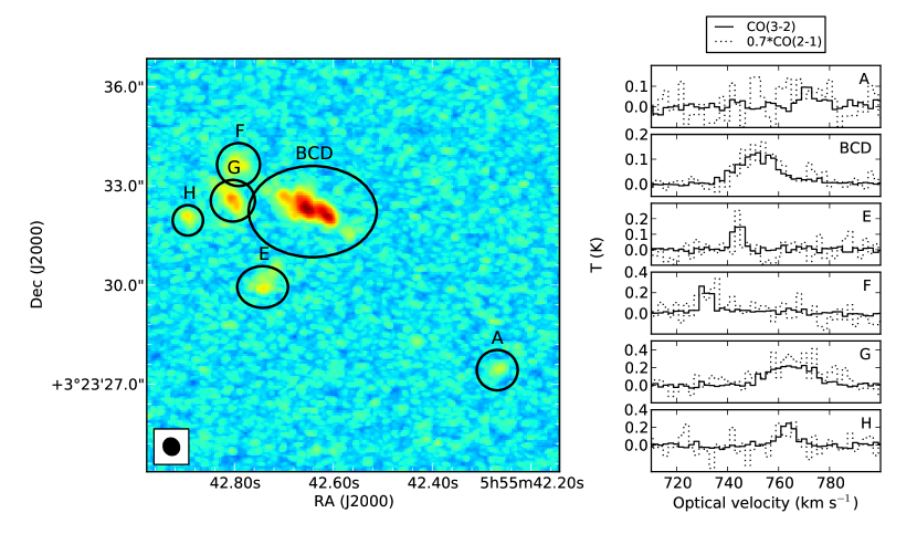
Figure 4.— $\rm{{}^{12}CO({3}-{2})}$ and $\rm{{}^{12}CO({2}-{1})}$ spectra from different regions in . On the left side of the image, the extraction regions are shown overlaid on a $\rm{{}^{12}CO({3}-{2})}$ image. These regions roughly correspond to the clouds identified in § III.2.1 and are labeled accordingly. The $\rm{{}^{12}CO({3}-{2})}$ and $\rm{{}^{12}CO({2}-{1})}$ spectra from each region are shown on the right. In general, the $\rm{{}^{12}CO({2}-{1})}$ emission is stronger than the $\rm{{}^{12}CO({3}-{2})}$ in , but the $\rm{{}^{12}CO({3}-{2})}$ observations have higher signal to noise. The ${\rm r_{32}}$ brightness temperature ratio is 0.7 for most regions, although cloud G has a lower ${\rm r_{32}}$ ratio of 0.5.

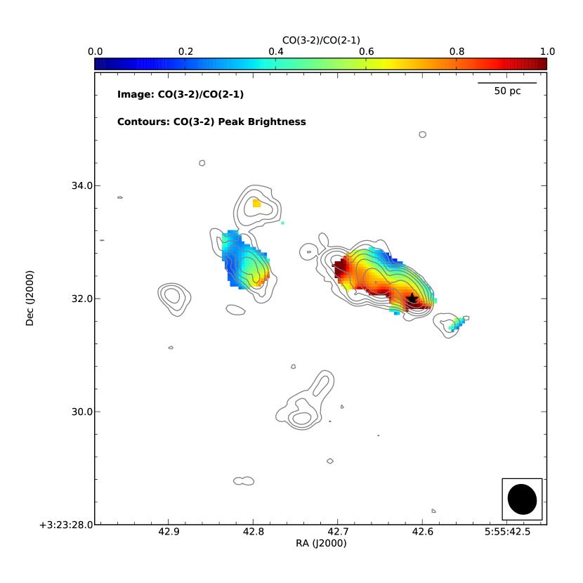
Figure 5.— The image shows the ${\rm r_{32}}$ brightness temperature ratio with contours showing $\rm{{}^{12}CO({3}-{2})}$ peak brightness temperature from Figure 3 overlaid. The location of the 1.3 cm continuum peak is indicated by a star. The ${\rm r_{32}}$ brightness temperature ratio is higher closer to the actively star-forming region in the center of .

The velocity field for  does not show strong evidence for rotation except for the main ridge of CO emission (Figure 6). The rest of the CO clouds appear to be relatively well separated in velocity space. Most of the clouds have velocity dispersions of $\sim$2 $\rm{km\,s}^{-1}$, except for the two bright emission peaks, which have larger velocity dispersions of $\sim$6 $\rm{km\,s}^{-1}$.

The $\rm{{}^{12}CO({3}-{2})}$ velocity field overlaps, but is not completely coincident with the H I velocity field (Figure 7). In the plane of the sky, the CO emission lies between two H I peaks, which we refer to as HI-I and HI-II. In velocity space, the CO clouds overlap the velocities of both peaks, although the CO main ridge appears to be more closely associated with the neutral hydrogen peak HI-I and the high velocity disperion region with HI-II.

Although  has not had its large-scale kinematics modeled in detail, its H I velocity field bears a strong resemblance to that of the merging galaxy NGC 7525, which has been modeled in detail by Hibbard & Mihos (1995). In particular, the H I velocity reversal within the field of view of the CO observations is consistent with gas from the progenitor galaxies flowing inward (c.f., Figure 6 in Hibbard & Mihos (1995), especially T=32 and T=40). It also agrees with the scenario presented in Brinks & Klein (1988) that the infalling gas from the progenitor systems may have led to the formation of molecular gas in and thus triggered the current burst of star formation in . High resolution N-body/SPH simulations of the merging galaxy Antennae have shown that a merger can produce an short-lived, off-center burst of star formation (Karl et al., 2010).

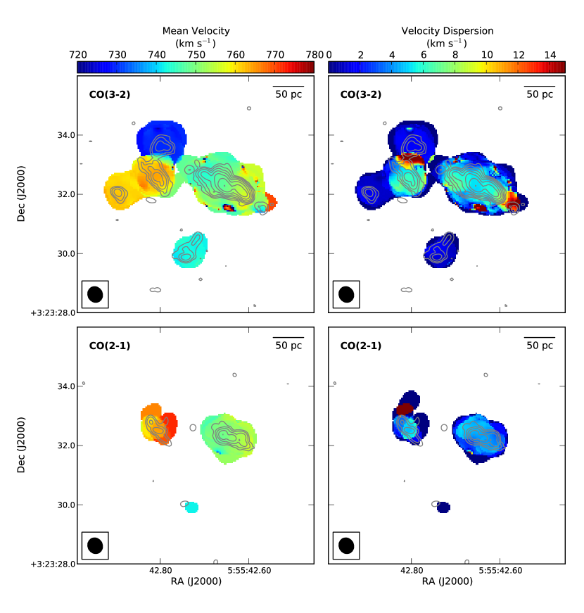
Figure 6.— Left column: The mean velocity for the $\rm{{}^{12}CO({3}-{2})}$ (top) and $\rm{{}^{12}CO({2}-{1})}$ (bottom) emission. The peak brightness temperature contours from Figure 3 are overlaid. Right column: The right column shows the velocity dispersion for the $\rm{{}^{12}CO({3}-{2})}$ (top) and $\rm{{}^{12}CO({2}-{1})}$ (bottom) emission. The peak brightness temperature contours from Figure 3 are overlaid. The velocity field for  shows little evidence for large scale rotation, except for the main CO emitting region. The velocity dispersions are highest in the brightest emitting CO clumps. In particular, the region near 05:55:42.8, 03:23:33, has an extremely high line width compared to the other regions ($\sim$6 $\rm{km\,s}^{-1}$ vs. $\sim$1-2 $\rm{km\,s}^{-1}$). The $\sim 10-14\rm{km\,s}^{-1}$ velocity widths just to the north of this region are due to the overlap of two different clouds. See Figure 12 and § III.2.1 for a discussion. We note that the region shown has been chosen to highlight the structure of the molecular gas in the central starburst. One cloud (Cloud A in the terminology of § III.2.1) falls outside. This cloud can be seen in the lower right hand corner of Figure 4.

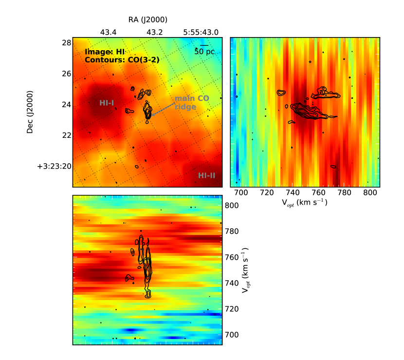
Figure 7.— A comparison of the H I and $\rm{{}^{12}CO({3}-{2})}$ data cubes. The cube has been rotated by 61 degrees so that the main ridge of CO emission runs up and down. The CO contours start at the three sigma noise level (0.087 $\rm{Jy\ beam^{-1}}\$) and increase by powers of two (0.174, 0.348, 0.696, …$\rm{Jy\ beam^{-1}}\$). The $\rm{{}^{12}CO({3}-{2})}$ emission lies between two H I peak (referred to here at HI-I and HI-II) and the velocities of the individual regions are coincident with the velocities of both H I peaks. The spatial distribution of the emission combined with the overlapping velocities suggests that the starburst in  may have been triggered by colliding gas clouds.

Approximately 30% of the total $\rm{{}^{12}CO({2}-{1})}$ emission in  is resolved out by our ALMA observations. The integrated $\rm{{}^{12}CO({2}-{1})}$ intensity for  from single dish observations with the IRAM 30m is 0.69 $\rm{K\,km\,s^{-1}}$ (Albrecht et al., 2004), while the integrated $\rm{{}^{12}CO({2}-{1})}$ intensity for the ALMA $\rm{{}^{12}CO({2}-{1})}$ cube smoothed to the same resolution (11″) is 27% lower (0.5 $\rm{K\,km\,s^{-1}}$; Figure 8). Although both the single dish and ALMA $\rm{{}^{12}CO({2}-{1})}$ profiles have similar central velocities, the ALMA $\rm{{}^{12}CO({2}-{1})}$ profile is missing emission in the line wings, suggesting that there is diffuse CO emission at non-systemic velocities. This result is consistent with CO observations in galaxies, in particular the Local Group dwarf galaxy IC 10 (Leroy et al., 2006).

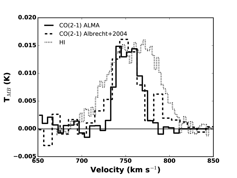
Figure 8.— A comparison of the ALMA $\rm{{}^{12}CO({2}-{1})}$ spectrum (solid black line) to a single dish $\rm{{}^{12}CO({2}-{1})}$ spectrum from the IRAM 30m (dashed line; Albrecht et al. 2004) shows that 38% of the $\rm{{}^{12}CO({2}-{1})}$ emission is resolved out of the ALMA observations. Although both profiles have similar central velocities, the ALMA $\rm{{}^{12}CO({2}-{1})}$ profile is missing emission in the line wings suggesting that there is diffuse CO emission at non-systemic velocities. Both $\rm{{}^{12}CO({2}-{1})}$ profiles peak near the peak of the neutral hydrogen profile (dotted line, maximum height scaled to 80% of the plot size), but have much narrower line widths.

III.1.2 Continuum Emission in

Dust is key to our picture of how CO emission changes with metallicity. As mentioned in the introduction, dust shields CO from disassociation, while ${\rm H_{2}}$ is able to self-shield. The reduced dust content found in low metallicity galaxies means less dust is available to shield CO, while the molecular gas itself is unaffected because H₂ self-shields. To explore the interplay of dust and CO emission in , we compile a submillimeter to centimeter continuum spectral energy distribution (SED) based on the ALMA data presented in this paper and archival centimeter VLA observations from Kepley et al. (2014). This SED contains synchrotron emission, free-free emission, and thermal emission from dust. Matched uv-coverage and resolution observations at multiple wavelengths are required to separate these components and characterize their properties.

Figure 9 shows matched beam and uv-coverage images for  from 6.2 cm through 870µm. The 6.2 cm, 3.5 cm, and 1.3 cm data were originally presented in Kepley et al. (2014) and have been re-imaged to match the uv-coverage and beam size of the ALMA observations. See Section II for details on the imaging process. The 3 mm continuum emission is compact and coincident with the free-free dominated 1.3 cm emission (Kepley et al., 2014). The emission is slightly extended at the highest (1 mm and 870µm) and lowest wavelengths (6.2 cm) indicating that the presence of emission from dust and synchrotron emission, respectively. We note that the morphology of the extended 870µm emission is similar to that of the $\rm{{}^{12}CO({3}-{2})}$ emission (overlaid as contours), while the 6.2 cm emission extends further south toward the older star-forming region (SSC-South using the terminology of Kepley et al., 2014). These images suggest that the millimeter and submillimeter continuum emission from this galaxy is dominated by free-free emission and that the dust does not dominate the continuum emission from  even at 870µm.

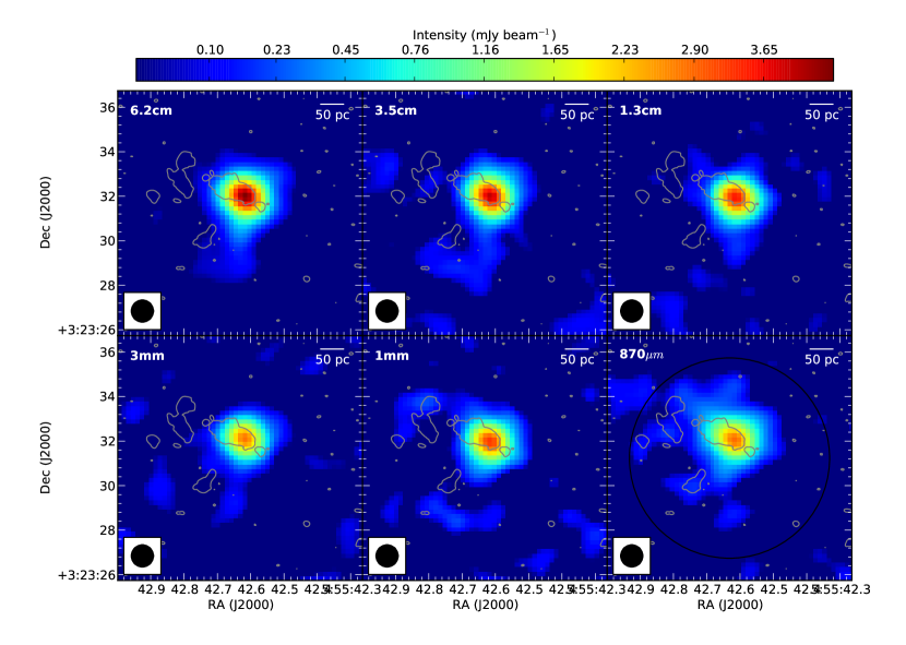
Figure 9.— Matched resolution and uv-coverage continuum images from 6.2 cm to 870µm of . The contours show the distribution of the $\rm{{}^{12}CO({3}-{2})}$ emission. The wavelength of the image is in the upper left, the image scale in the upper right, and the beam in the lower left. All six images have the same stretch to bring out the changes in extent and brightness of the emission as a function of wavelength. The 1 mm and 3 mm emission is compact and coincident with the 1.3 cm emission, which is dominated by free-free emission (Kepley et al., 2014). The slightly extended emission at 6.2 cm and 870µm is due to the presence of synchrotron and dust emission, respectively. The relatively consistent morphology and brightness of the continuum emission across all bands suggests that the continuum emission in  is dominated by free-free emission even up to 870µm. The large black circle in the bottom right panel shows the aperture used to extract the continuum flux densities.

To quantify this further, we have extracted the continuum spectral energy distribution (SED) in a $9\arcsec$ diameter aperture centered at (5:55:42.63161, 3:23:31.2387). The measured flux densities are given in Table 5. We fit a simple two power law model to these values:

$$\frac{S}{S_{0}}=p_{th}\left(\frac{\nu}{\nu_{0}}\right)^{-0.1}+(1-p_{th})\left(\frac{\nu}{\nu_{0}}\right)^{\alpha_{nt}}$$ (1)

where $S$ is the flux density at frequency $\nu$ compared to the flux density ($S_{o}$) at a fiducial frequency ($\nu_{0}$), $p_{th}$ is the thermal fraction emission, and $\alpha_{nt}$ is the spectral index of the non-thermal emission. The aperture was selected to completely encapsulate the continuum emission at all frequencies. For our fit, we excluded the 1 mm and 870µm data since these data points contain a contribution from dust and set $\nu_{0}$ to 4.86 GHz. The fit is shown in Figure 10. The best fit thermal fraction is 0.34 with a range of 0 to 0.7 and the best fit non-thermal spectral index is -0.3 with a range of -0.21 to -0.87. The reduced $\chi^{2}$ value for the best fit is 0.18. This fit shows that, up to 100 GHz, the emission from  is a combination of free-free and non-thermal emission. Only at frequencies greater than 100GHz do we see any indications of dust emission, and the contribution at those frequencies is relatively low: even at 870µm, the dust emission is only 50% of the total. We note that the present fit contains a greater contribution from synchrotron emission than the fit to only the VLA data points shown in Kepley et al. (2014). This difference is due to the different uv-coverage and resolution of the images. Here we have emphasized sensitivity to large-scale flux at the expense of resolution, making the synchrotron emission more pronounced because it is typically on larger scales. We note that the spectral index of the synchrotron emission is consistent between the old and new fits.

Table 5Radio/Submillimeter Continuum Spectrum of II Zw 40

	Frequency	Flux Density
Wavelength	GHz	mJy
6.2 cm	4.86	$9.4\pm 1.9$
3.5 cm	8.46	$7.5\pm 1.5$
1.3 cm	22.46	$7.1\pm 1.4$
2.7 mm	112.70	$4.7\pm 0.9$
1.3 mm	233.38	$5.9\pm 1.2$
870.0 µm	344.88	$7.7\pm 1.5$

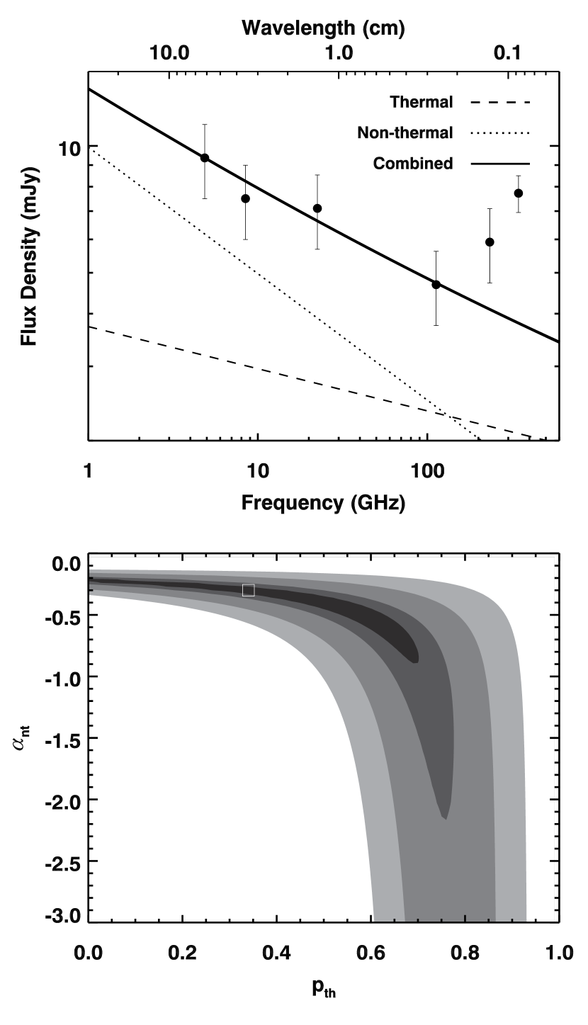
Figure 10.— Top: The global continuum spectral energy distribution for  from centimeter to millimeter wavelengths derived from matched uv-coverage and resolution images from the VLA (Kepley et al., 2014) and ALMA (this paper). The emission in this range consists of three components: synchrotron, which is strongest at lower frequencies, free-free, which has a mostly flat spectrum, and dust, which is strongest at the highest frequencies in this plot. The lines show the best two power law fit to the data points less than 230GHz. This plot shows that the synchrotron and thermal emission both contribute to the continuum spectral energy distribution at frequencies less than 100GHz and that only the 1 mm and 870µm points include a contribution from dust. Bottom: Reduced $\chi^{2}$ values for fits as a function of thermal fraction and non-thermal spectral index. The contours are 1.25, 2, 5, and 10 times the minimum reduced $\chi^{2}$ value. Our best fit value is shown as a white square.

To further explore the dust content of , we have added the mid- and far-infrared Herschel photometry and resulting fit from Rémy-Ruyer et al. (2013) to the ALMA and VLA data points to better capture the peak of the dust emission (Figure 11). To obtain an estimate of the dust mass from these points, we attempted to fit a modified black body to the dust emission:

$$F_{\nu}=\frac{M_{dust}\kappa(\lambda_{0})}{D^{2}}\left(\frac{\lambda}{\lambda_{0}}\right)^{-\beta}B_{\nu}(\lambda,T)$$ (2)

where $M_{dust}$ is the dust mass, $\kappa(\lambda_{0})$ is the dust absorption coefficient at the reference wavelength $\lambda_{0}$, $D$ is distance to the object, $\lambda$ is the observed wavelength, $\beta$ is the dust emissivity index, and $B_{\nu}(\lambda,T)$ is the Planck function. We assume a value for $\kappa(\lambda_{0})$ of 4.5 ${\rm m^{2}\,kg^{-1}}$. This value is based on the models of Zubko et al. (2004) and is the same value used in Rémy-Ruyer et al. (2013). All attempts to fit a modified blackbody through both the ALMA and Herschel data points yielded poor fits. The failure of these fits is most likely due to either large-scale dust emission being resolved out by ALMA or to the large difference between the apertures used for the Herschel and ALMA photometry: 132″ versus 9″. Although we could increase the aperture size for the ALMA data, the Herschel aperture is larger than our ALMA field of view (see Table 4).

Given our inability to fit both the ALMA and Herschel points simultaneously, we derive an estimate of the dust mass using only the ALMA data by setting $\beta$ and the temperature to the values derived by Rémy-Ruyer et al. (2013): 1.71 and 33K. We obtain a dust mass of $(1.8\pm 0.2)\times 10^{4}\ \rm{M}_{\odot}$, which is a factor of 10 less than the dust mass estimated by Rémy-Ruyer et al. (2013): $1.9\times 10^{5}\ \rm{M}_{\odot}$. We note that fixing the $\beta$ value only has a minor effect on the derived mass. Changing $\beta$ from 1.71 to 2.0 changes the mass by less than 10%. In addition, since our observations are on the Raleigh-Jeans tail of the dust distribution, our derived dust mass is only minimally affected by the assumed temperature: the mass-weighted temperature would need to have a factor of two uncertainty to produce a factor of two uncertainty in the mass .

Figure 11.— The global continuum spectral energy distribution for  from the centimeter (VLA; Kepley et al., 2014), millimeter/submillimeter (ALMA), and the far-infrared (Herschel; Rémy-Ruyer et al., 2013). We include a modified black body fit to the 1mm and 870µm points as well as the fit to the Herschel data points from Rémy-Ruyer et al. (2013) as a dot-dot-dash line. The VLA and ALMA points are shown as circles and the Herschel points are shown as inverted triangles. For the fit to the ALMA data points, the temperature and $\beta$ were fixed to the value derived from the Herschel measurements by Rémy-Ruyer et al. (2013) because this value is largely determined by the value of the dust peak traced by Herschel. We find a dust mass of $1.9\times 10^{4}$ $\rm{M}_{\odot}$, which is a factor of 10 lower than the dust mass derived using only Herschel photometry by Rémy-Ruyer et al. (2013). This result suggests that either a large amount of dust emission is being resolved out or that there is significant dust emission outside the aperture used for the ALMA photometry.

Armed with a dust mass for , we can calculate its gas-to-dust ratio ($\delta_{GDR}$), which links the gas and dust content within the galaxy. The gas-to-dust ratio is used as an alternative way to trace the molecular gas content of a galaxy (e.g., Israel, 1997; Leroy et al., 2011; Sandstrom et al., 2013). Here we use archival VLA neutral hydrogen data (van Zee et al., 1998) and the molecular gas measurements from Section III.2.2 to calculate the gas-to-dust ratio in  and compare it to theoretical estimates of the gast-to-dust ratio in low metalllicity systems.

The gas-to-dust ratio is defined as

$$\delta_{GDR}=\frac{\alpha_{co}{\rm L_{CO}}+M_{HI}}{M_{dust}}$$ (3)

where $\alpha_{co}$ is the CO-to-H₂ conversion factor in $\rm M_{\odot}(\rm K\,\rm{km\,s}^{-1}\,pc^{2})^{-1}$, ${\rm L_{CO}}$ is the CO luminosity in $\rm K\,\rm{km\,s}^{-1}\,pc^{2}$, and $M_{HI}$ and $M_{dust}$ are the neutral hydrogen and dust masses, respectively, in $\rm{M}_{\odot}$. Here we are defining $\delta_{GDR}$ in terms of masses, instead of surface densities, which requires us to match the apertures used to measure each quantity. In the same 9″ aperture as we used to measure the continuum SED, we measure an $M_{HI}$ of $6.0\times 10^{6}$ $\rm{M}_{\odot}$ and a $\rm{{}^{12}CO({3}-{2})}$ luminosity of $2.1\times 10^{5}$ $\rm K\,\rm{km\,s}^{-1}\,pc^{2}$, which corresponds to a $\rm{{}^{12}CO({1}-{0})}$ luminosity of $3.8\times 10^{5}$ $\rm K\,\rm{km\,s}^{-1}\,pc^{2}$ using an ${\rm r_{31}}$value of 0.54. From § III.2.2, we have estimates from $\alpha_{co}$ that range from 18.1 $\rm M_{\odot}(\rm K\,\rm{km\,s}^{-1}\,pc^{2})^{-1}$ to 150.5 $\rm M_{\odot}(\rm K\,\rm{km\,s}^{-1}\,pc^{2})^{-1}$. These values give a range for $\delta_{GDR}$ of 720 to 3500. We note that, if we are resolving out a significant amount of continuum emission, our $\delta_{GDR}$ will be overestimates (because we will have underestimated the dust content). The lower end of our estimated range range is similar to the Rémy-Ruyer et al. (2014) predicted value (645-660, depending on assumptions about $\alpha_{co}$). It is greater than, but still within an order of magnitude, of the $\delta_{GDR}$ predicted by the Leroy et al. (2011) (330) and the range of values given for blue compact dwarfs of similar metallicity by Hunt et al. (2014). We do not see any evidence for the dichotomy seen in Hunt et al. for the $\delta_{GDR}$ ratios for the very low metallicity galaxies I Zw 18 and SBS0335-052, although the metallicity of  is ten times higher than in both of those systems.

III.2. The Molecular Clouds Fueling the Starburst within

Observations of low metallicity galaxies with the spatial and spectral resolutions necessary to resolve individual molecular clouds are rare because of the faint nature of the CO emission in these galaxies. Previously, only a dozen or so galaxies had bright enough CO to obtain high resolution observations with sufficient signal to noise, e.g., Table 1 in Bolatto et al. (2008). These galaxies were typically limited either to very nearby galaxies or to those with relatively high metallicities (and thus brighter CO). The sensitivity and resolution of ALMA observations, like those presented here for , allow us to measure for the resolved molecular cloud properties in fainter and more extreme low metallicity systems, and compare them to the properties of molecular clouds in other galaxies.

Originally motivated by observations in the Milky Way (Larson, 1981; Solomon et al., 1987), the so-called Larson’s laws are commonly used to quantify and compare the giant molecular cloud properties in galaxies. The first relationship states that the linewidth of a molecular cloud scales with its size and is generally referred to as the size-linewidth relationship. The second relationship shows that the CO luminosity of a molecular cloud is correlated with its virial mass. This relationship is typically used to infer the conversion factor between the observed CO luminosity and the molecular gas mass of a cloud, under the assumptions that virial equilibrium holds and that the CO traces the full extent of the molecular gas. The final relationship, which is a consequence of the first two, states that molecular clouds all have approximately the same surface density. These relationships have been shown to be sensitive to the resolution and sensitivity limits of the data and the methods used to measure the cloud properties (e.g., Wong et al., 2011; Hughes et al., 2013). However, they continue to provide the basic framework for understanding giant molecular cloud populations.

In this section, we identify individual molecular clouds within , quantify their properties, and compare these properties to those of molecular clouds in other environments. Our comparison sample was selected to span a wide range of cloud properties and environments. It includes cloud samples from the Milky Way disk (Heyer et al., 2009), the center of the Milky Way (Oka et al., 2001), the nearby low metallicity irregular Large Magellanic Cloud (Wong et al., 2011), the Local Group dwarf starburst IC 10 (Leroy et al., 2006), the major merger referred to as the Antennae (Whitmore et al., 2014, Leroy et al. in prep), and the nuclear starburst galaxy NGC 253 (Leroy et al., 2015). To mitigate the effects of varying sensitivity and resolution, we have focused on comparison cloud samples whose original observations have relatively high ($\lesssim 50$pc) resolution and good surface brightness sensitivity and where the algorithms used to determine the cloud properties were similar to those used here, i.e., variants on the algorithm in Rosolowsky & Leroy (2006).

III.2.1 Measuring the Cloud Properties

We used the cprops algorithm (Rosolowsky & Leroy, 2006) to identify individual molecular clouds within  and calculate their properties. This algorithm identifies significant emission within a cube using a dilated mask and associates this emission with individual clouds using a modified watershed algorithm. The $\rm{{}^{12}CO({3}-{2})}$ data cube was used to identify the clouds because it has the highest signal-to-noise out of all our data sets. To identify significant emission, we used a three dimensional noise cube and required the emission to be greater than 5$\sigma$ in two adjacent channels to generate an initial mask. All pixels connected to this initial mask down to a 2$\sigma$ level were then added to the mask. To decompose the emission into individual clouds, we used a box of 0.35″ by 0.35″ by 6 $\rm{km\,s}^{-1}$; 0.35″ is 17pc at the adopted distance of . We rejected regions with a contrast less than 1.5$\sigma$ and areas less than the FWHM of the beam. We note that emission that can be associated with more than one cloud is not included in the mask. The measured cloud properties have been extrapolated down to 0K and corrected for the angular and velocity resolution of the data as described in Rosolowsky & Leroy (2006).

Our results do not depend strongly on the cube used for the decomposition, decomposition algorithm, or decomposition parameters. The cube decompositions for both the $\rm{{}^{12}CO({2}-{1})}$ and $\rm{{}^{12}CO({3}-{2})}$ both identify the brightest clouds. The main difference between the two cloud identifications is that the $\rm{{}^{12}CO({3}-{2})}$ emission spans a larger continuous area at high signal to noise; the $\rm{{}^{12}CO({2}-{1})}$ emission appears to be moderately clumpier because only the brightest peaks remain at high signal to noise. An alternative decomposition algorithm – clumpfind (Williams et al., 1994) – produces similar results when applied to our data to those generated by the cprops algorithm. Finally, changing the decomposition parameters only affects how many clouds the main molecular ridge is separated into. Depending on the parameters chosen, the ridge can either be identified as a single large cloud or up to four different clouds. We have tuned these parameters to match the number of clumps that can be distinguished by eye in the position-velocity plot of the $\rm{{}^{12}CO({3}-{2})}$ emission (Figure 12).

The cloud identifications are shown in Figure 12 overlaid on the $\rm{{}^{12}CO({3}-{2})}$ data and the cloud properties in Table 6. Since the clouds are largely Gaussian, the final cloud sizes and luminosities (and thus their associated properties like mass, etc) were taken from the Gaussian fit to the cloud sizes with the beam and channel width deconvolved. For clouds that were unresolved, we derive an upper limit on the radius of the cloud by calculating the diameter of a circle that has the same area as the area at half-maximum covered by the cloud.

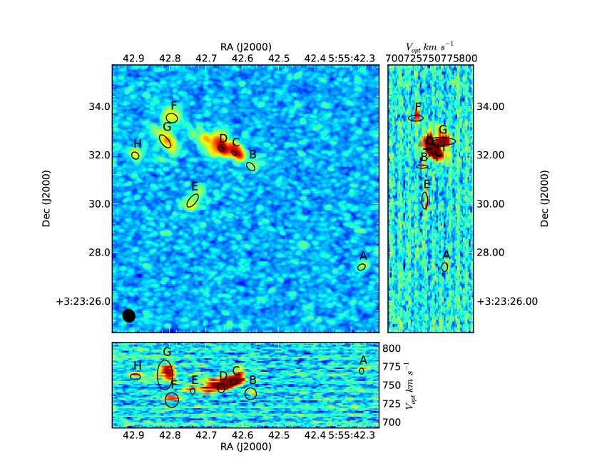
Figure 12.— Clump assignments as measured using the cprops algorithm overlaid on an image of the $\rm{{}^{12}CO({3}-{2})}$ cube in RA/Dec space (large square), RA/velocity space (bottom rectangle), and Dec/Velocity space (left rectangle).

Monte Carlo simulations were used to determine the errors on the measured properties. We added Gaussian noise with the same properties as the noise cube used to mask the emission to the image cube and calculated the properties of the resulting clumps. After 100 iterations, we calculated the standard deviation of the resulting clump properties and used this value as the error. For flux-related values, we added the errors on the derived flux (10% at 870µm and 20% at 1 mm; see Section II) in quadrature with the errors derived from the Monte Carlo simulations.

In the literature, the $\rm{{}^{12}CO({1}-{0})}$ transition is the most common tracer of molecular gas. To compare our data to the $\rm{{}^{12}CO({1}-{0})}$ data in the literature, we scale our $\rm{{}^{12}CO({3}-{2})}$ emission for all clouds, except cloud G, to the expected $\rm{{}^{12}CO({1}-{0})}$ value using a 10K blackbody, which is consistent with the line ratios for the entire galaxy (see Section III.1). Since cloud G has a significantly different value of ${\rm r_{32}}$, we scale its $\rm{{}^{12}CO({3}-{2})}$ emission to the expected $\rm{{}^{12}CO({1}-{0})}$ value using a 6K blackbody, which is consistent with the ratio seen in that cloud (again see Section III.1).

III.2.2 The CO-to-H₂ Conversion Factor

Since CO is used as the primary tracer of molecular gas beyond the Local Group, quantifying the relationship between CO emission and the amount of molecular gas in different environments is key for understanding the role of molecular gas in star formation throughout cosmic time. In the Milky Way, this conversion factor is typically 4.3 $\rm M_{\odot}(\rm K\,\rm{km\,s}^{-1}\,pc^{2})^{-1}$ (Bolatto et al., 2013). However, it is a factor of $\sim 5$ lower in starburst galaxies like LIRGs and ULIRGs and several times higher in low metallicity systems (Bolatto et al., 2013). As detailed in the introduction, the high $\alpha_{co}$ values in the latter systems are due to reduced dust shielding for the CO (e.g. Bolatto et al., 2008; Leroy et al., 2011). In contrast, the lower values of $\alpha_{co}$ in starburst galaxies are due to increased CO luminosity due to higher gas temperatures and broader velocity widths (e.g., Narayanan et al., 2012).

Assuming that the clouds in  are in virial equilibrium, we can derive $\alpha_{co}$ for molecular clouds within  by comparing the virial masses of the clouds with their CO luminosities. For , we derive a value for $\alpha_{co}$ of $18.1\pm 0.5$ $\rm M_{\odot}(\rm K\,\rm{km\,s}^{-1}\,pc^{2})^{-1}$ by fitting a slope to the resolved giant molecular cloud population in ${\rm L_{CO}}$-$M_{vir}$ space (Figure 13). This value is approximately four times higher than the Milky Way value, but is consistent with $\alpha_{co}$ values in other dwarf starburst galaxies derived using resolved CO observations (Bolatto et al., 2008). Two exceptions to this trend are Clouds E and C. Cloud E, the faintest cloud with virial mass estimate in our sample, is a more diffuse molecular cloud located south of the main star-forming region. However, given the errors on the associated luminosity, the $\alpha_{co}$ value for this cloud is broadly consistent with the derived $\alpha_{co}$ value above. Cloud C is associated with the central starburst. This cloud has the lowest ratio of virial mass to CO luminosity, suggesting that its $\alpha_{co}$ value may be more like that of a starburst galaxy. However, given that we only have an upper limit on its virial mass, this remains a suggestion rather than a definite statement.

Our $\alpha_{co}$ estimate is dependent on our assumed value of ${\rm r_{31}}$. If ${\rm r_{31}}$ is higher, i.e., the clouds are hotter, then the estimated $\rm{{}^{12}CO({1}-{0})}$ values will be smaller and the fitted $\alpha_{co}$ factor higher. If ${\rm r_{31}}$ is lower, i.e., the clouds are cooler, then the estimated $\rm{{}^{12}CO({1}-{0})}$ values will be larger and the fitted $\alpha_{co}$ factor lower. We note that we would require an ${\rm r_{31}}$ value of 0.12, implying an extremely cold cloud temperature ($\lesssim 3K$), for the $\alpha_{co}$ value derived from our data to be equal to the Milky Way value. This value is clearly at odds with the line ratios seen in  (§ III.1.1). We include the statistical errors on ${\rm r_{31}}$ (see Section III.1.1 for a dicussion) in our $\rm{{}^{12}CO({1}-{0})}$ luminosities in Figure 13. Based the errors for ${\rm r_{31}}$ ranges, it is unlikely that our derived $\alpha_{co}$ would be off by more than the error in ${\rm r_{31}}$ ($\sim$ 30%), although the unresolved points only have upper limits for their virial masses, and thus could drive the $\alpha_{co}$ factor lower.

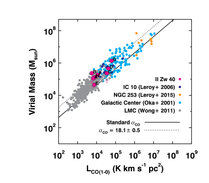
Figure 13.— The virial mass of the molecular clouds identified in § III.2.1 as a function of their CO luminosity. We also include clouds from our comparison samples: the Local Group dwarf starburst IC 10 (Leroy et al., 2006), the nuclear starburst NGC 253 (Leroy et al., 2015), the Milky Way center (Oka et al., 2001), and the Large Magellanic Cloud (Wong et al., 2011). Assuming that the clouds in  are in virial equilibrium, the relationship between these two quantities yields an estimate of the CO-to-H₂ conversion factor ($\alpha_{co}$). A fit to the resolved molecular clouds in this plot suggests that $\alpha_{co}$ is approximately four times its value in the Milky Way. This conversion factor is similar to the conversion factors seen in other low metallicity galaxies, rather than the conversion factors seen in more massive starbursting galaxies (LIRGs/ULIRGs).

In low metallicity systems, estimates of the CO-to-H₂ conversion factor derived using virial masses are systematically lower than the estimates derived using IR observations (e.g., Leroy et al., 2011). This offset is thought to be caused by the reduced dust content of low metallicity systems: dust is the primary shielding mechanism for CO, but H₂ molecules are able to self-shield. At solar metallicity, the H₂ and CO emission have similar physical extents. As the metallicity decreases, the amount of dust decreases, which decreases the shielding available for CO, driving it toward the centers of the molecular clouds (Bolatto et al., 2008). The molecular gas not traced by CO is commonly referred to as the “dark” molecular gas (Wolfire et al., 2010).

The systematic differences between CO and IR-based $\alpha_{co}$ estimates suggests that the $\alpha_{co}$ estimate for  derived here may underestimate the true $\alpha_{co}$ value for . Ideally, we would compare the CO-based $\alpha_{co}$ estimate for  to a measured IR-based value of $\alpha_{co}$ using far-infrared dust maps and neutral hydrogen (Leroy et al., 2011; Sandstrom et al., 2013). However, the spatial resolutions of the best possible neutral hydrogen and far-infrared observations are far too low to resolve the central star-forming region of : the maximum feasible resolution of neutral hydrogen observation is $\sim 5\arcsec$, while far-infrared observations from Herschel have resolutions ranging from $\sim 5\arcsec$ to $\sim 30\arcsec$. Although the 870µm continuum data presented here could be used to provide an estimate for the dust emission, the extended dust emission is only seen in the heavily tapered, low resolution image, not in an image with uv-coverage and resolution matched to that of the $\rm{{}^{12}CO({3}-{2})}$ observations.

We can use the total CO luminosity and derived dust mass along with an estimate of the gas-to-dust ratio ($\delta_{GDR}$) to estimate a value of $\alpha_{co}$ for the central star-forming region of . Rémy-Ruyer et al. (2013) provide an empirical estimate of the $\delta_{GDR}$ as a function of metallicity. For the metallicity of  (8.09; Guseva et al., 2000), the estimated $\delta_{GDR}$ is between 645-660. Here we adopt a mid-range value of 650. The total estimated $\rm{{}^{12}CO({1}-{0})}$ luminosity in this region (adopting the typical value of ${\rm r_{31}}$ in § III.2.1) is $3.8\times 10^{5}\ \rm K\,\rm{km\,s}^{-1}\,pc^{2}$, the dust mass for the central star-forming region is $1.4\times 10^{4}\ \rm{M}_{\odot}$ (see § III.1.2), and the neutral hydrogen mass for the same region is $6.0\times 10^{6}\ \rm{M}_{\odot}$. These values give an estimate of $\alpha_{co}$ of 14$\rm M_{\odot}(\rm K\,\rm{km\,s}^{-1}\,pc^{2})^{-1}$, which is consistent with the CO-based $\alpha_{co}$ estimate. However, this value is a lower limit, given that we may be underestimating the dust mass because we are resolving out continuum emission.

Finally, we can use the simple photodissociation model developed by Wolfire et al. (2010) to estimate $\alpha_{co}$. In this model, $\alpha_{co}$ depends strongly on the column density of the gas, which for resolved observations depends on the metallicity and integrated CO line intensity. Thus, with our resolved observations, we can independently derive an estimate for $\alpha_{co}$ based only on these two readily observed quantities. In the Appendix, we derive an expression for the ratio of $\alpha_{co}$ at a metallicity $Z$ to $\alpha_{co}$ at solar metallicity as a function of CO line intensity $W_{CO}$ and metallicity ($Z$). Taking values appropriate for  ($Z=0.2$ and $W_{CO(1-0)}$ between 0.85 and 2.6 $\rm{K\,km\,s^{-1}}$), we find that, according to this model, the $\alpha_{co}$ for  should be 15 to 35 times higher than the Milky Way value, lending support to the idea that the $\alpha_{co}$ value derived using virial mass estimates is indeed a lower limit on the $\alpha_{co}$ value in this galaxy. However, there is significant scatter in the CO line intensity values, suggesting that the assumption of constant CO surface brightness leading to constant molecular gas surface densities may not be valid. For , this leads to a factor of two scatter in the estimated $\alpha_{co}$value. We will explore the assumption of constant CO surface density in detail in a later section (§ III.2.4).

Our resolved observations provide the rare opportunity to compare our cloud-based estimates of $\alpha_{co}$ to model predictions of global $\alpha_{co}$ values in low metallicity environments. Narayanan et al. (2012) uses the results of Wolfire et al. (2010) to model populations of molecular clouds within galaxies. From their simulations, they derive a relationship between the surface brightness of CO and the metallicity of a galaxy. With our cloud-scale resolution, we are in a unique position to test the veracity of these models at low metallicity. Using their Equation 7, the metallicity of   and the average $\rm{{}^{12}CO({1}-{0})}$ surface brightness of its clouds from Figure 14 (1.8 $\rm{K\,km\,s^{-1}}$), we derive an estimate of $\alpha_{co}$ of 17.5, which is close to value we derive from the virial mass estimate. However, we note that the value derived here is in the low CO surface brightness limit where, according to Narayanan et al. (2012), the properties of the molecular clouds depend less on environment. Given the observational evidence for larger $\alpha_{co}$ values in low-metallicity galaxies, we suggest that the $\alpha_{co}$ values derived from these models may be underestimates for low metallicity systems.

The preceding discussion of $\alpha_{co}$ estimates has ignored any time-variable effects on the $\alpha_{co}$ value, which may be essential for starbursting systems like . Bursts of star formation like those found in  may increase the dichotomy between the dust-derived and virial-derived $\alpha_{co}$ estimates by increasing CO photodissociation. In pre-starburst systems, these $\alpha_{co}$ estimates may be closer together due to the reduced flux of ionizing photons.

III.2.3 The Molecular Star Formation Efficiency

With our estimates for $\alpha_{co}$ in hand, we can now derive a value for the molecular star formation efficiency within , which characterizes how well this galaxy is able to turn molecular gas into stars. For the entire central region, ${\rm L_{CO(3-2)}}$ is $2\times 10^{5}\ \rm K\,\rm{km\,s}^{-1}\,pc^{2}$, which corresponds to an ${\rm L_{CO(1-0)}}$ of $3.8\times 10^{5}\ \rm K\,\rm{km\,s}^{-1}\,pc^{2}$ using the appropriate value for ${\rm r_{31}}$ (see § III.1.1). To obtain an upper limit on the star formation efficiency, we use our largest estimate for $\alpha_{co}$: 150.5 $\rm M_{\odot}(\rm K\,\rm{km\,s}^{-1}\,pc^{2})^{-1}$. The star formation rate in the central region of  is 0.34 $\rm{M}_{\odot}\,yr^{-1}$ (Kepley et al., 2014). These values yield a molecular star formation efficiency for  of $6\times 10^{-9}\,{\rm yr}^{-1}$, which is approximately 10 times higher than the average star formation efficiencies found in nearby spirals (Leroy et al., 2008).

If we use the virial-based $\alpha_{co}$ estimate, we derive an even higher molecular star formation efficiency: $4\times 10^{-8}\,{\rm yr}^{-1}$. This value is two orders of magnitude higher than in normal spirals and is similar to the star formation efficiencies seen in starburst galaxies (Daddi et al., 2010). However, by using the virial-derived $\alpha_{co}$ measurement, we are only including the molecular gas emission from deep inside the molecular cloud rather than averaging the molecular gas over kpc regions as in Leroy et al. (2008) and Daddi et al. (2010). Therefore, the molecular star formation efficiency calculated using a virial-based $\alpha_{co}$ estimate may be expected to be higher because it includes only the densest molecular gas regions where stars are more likely to form, while the values given in Leroy et al. (2008) and Daddi et al. (2010) average over many of these such regions and also include diffuse molecular gas.

The molecular star formation efficiency values derived above do not take into account the star formation history of  and the effect of its young massive clusters on their surrounding molecular gas. In more massive galaxies, the star formation rate is roughly constant with time over kpc-sized regions or we would not see the observed level of agreement between different star formation rate tracers (Murphy et al., 2011, 2012; Leroy et al., 2012). A continuous star formation rate ensures a steady conversion of gas into stars, allowing the present star formation in these systems to be linked to the remaining gas supply. However, in the case of interacting systems like , their star formation varies with both position and time and their bursts of star formation dissociate the leftover molecular gas. These time dependent effects mean that one cannot directly link the present day star formation with the past molecular gas supply.

We suggest that the high molecular star formation efficiency seen in  is due to its rapidly changing, merger-driven star formation history, not an intrinsically high molecular star formation efficiency. For example, in , the massive cluster associated the molecular gas (SSC-N) is young ($\lesssim$ 5Myr; Kepley et al., 2014). The cluster immediately to the south (SSC-S) is much older (9.5 Myr) and shows no associated molecular gas. We can also see clear signs that SSC-N is destroying the surrounding molecular gas. As we saw in § III.1.1, the ${\rm r_{31}}$ ratios are elevated here, indicating hotter gas. Higher resolution observations of the ionized gas within cloud C show filamentary structures, suggesting that ionizing radiation from SSC-N is destroying its molecular envelope (Kepley et al., 2014). Therefore, understanding the observed molecular star formation efficiencies in galaxies like  requires careful modeling of the star formation histories in these systems and the effects of the young massive clusters on the surrounding interstellar medium.

III.2.4 CO Surface Brightnesses and Mass Surface Densities

As discussed in §III.2, there is increasing evidence that the third Larson’s relation – molecular clouds have constant mass surface densities – is the result of the sensitivity and resolution limits of earlier surveys (Wong et al., 2011; Hughes et al., 2013). However, there do appear to be systematic offsets in the surface density of clouds between galaxies that have been attributed to differences in pressure (Hughes et al., 2013). In this section, we explore whether the molecular clouds within  have constant surface brightnesses and thus constant mass surface densities and compare these quantities to the surface brightnesses and surface densities in our comparison sample.

Figure 14 compares CO luminosity as function of cloud size for both  and the comparison sample. The left panel includes the measured $\rm{{}^{12}CO({3}-{2})}$ values for both the Antennae and   while the right panel has the estimated $\rm{{}^{12}CO({1}-{0})}$ values for  and the measured $\rm{{}^{12}CO({1}-{0})}$ values from galaxies in the comparison sample. Lines of constant surface brightness are shown as dot-dashed lines and the sensitivity and resolution limit of the  data is shown as a dotted line.

These plots show that, for the most part, the clouds in  have lower CO surface brightnesses than clouds in the Galactic Center, NGC 253, and the Antennae. These surface brightnesses are comparable to clouds found in the LMC and IC 10. Therefore, the globally low CO luminosity in  is due to low overall CO surface brightnesses, not a few high surface brightness clouds with very low filling factors. If  is representative of dwarf starburst galaxies as a whole, then we can expect that they will also have low overall CO surface brightnesses. The exception to the low-surface brightness trend is Cloud C: it has a comparable surface brightness to clouds in the Antennae, the Galactic Center, and NGC 253. This cloud is also the only cloud in  with active star formation.

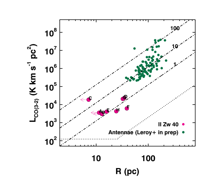
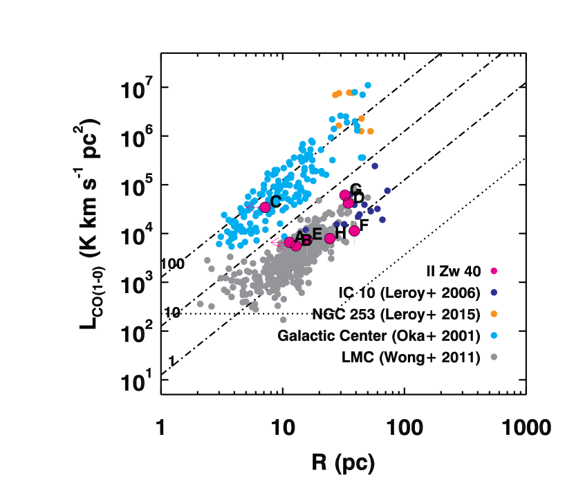
Figure 14.— ${\rm L_{CO(3-2)}}$ (left) and ${\rm L_{CO(1-0)}}$ (right) in  and the comparison sample as a function of cloud radius. The dash-dotted lines are lines of constant surface brightness (1, 10, 100 $\rm{K\,km\,s^{-1}}$) and the dotted line indicates the sensitivity and resolution limits of the  data. In general, the clouds in  have lower CO surface brightnesses than the clouds seen in higher metallicity galaxies like the Antennae, NGC 253, and the center of our own Galaxy. The clouds in  have similar surface brightness to the clumps in the LMC and the Local Group dwarf starburst IC 10. The one exception is cloud C, which higher CO surface brightness comparable to the CO surface brightnesses in the Galactic Center, NGC 253, and the Antennae. This cloud is also the only cloud in  with active star formation.

Figure 14 also shows that the molecular clouds within a particular galaxy tend to have similar CO surface brightness, i.e., the clouds fall along a diagonal line in ${\rm L_{CO}}$ versus radius plots. For our data, however, any systematic variations in the CO surface brightness could also be due to differences in $\alpha_{co}$, not just differences in the mass surface density of clouds, To account for the difference $\alpha_{co}$ values, we plot the CO-derived cloud mass versus radius for  and the comparison sample as a function of size in Figure 15. This plot shows that the CO-derived mass surface densities of molecular clouds within  are on average higher than those in the LMC or IC 10 and are comparable to the CO-derived mass surface densities of clouds within the Antennae and the Galactic Center. Based on these results, the low CO luminosities seen in  are the result of higher $\alpha_{co}$ factors rather than low surface density molecular gas, showing that the clouds within  have normal mass surface densities compared to clouds in other galaxies.

Systematic uncertainities with the values of $\alpha_{co}$ and ${\rm r_{31}}$ will impact the location of the  clouds on these plots. Smaller values of ${\rm r_{31}}$, which imply colder molecular gas, will move the clouds to higher ${\rm L_{CO}}$ values in the right panel of Figure 14. For the mass versus radius plots, the ${\rm r_{31}}$ and $\alpha_{co}$ affect the result in opposite directions: increasing ${\rm r_{31}}$ leads to lower ${\rm L_{CO}}$ values and thus lower mass surface densities, while increasing $\alpha_{co}$ leads to higher mass surface densities. Given that the values we derive for ${\rm r_{31}}$ and $\alpha_{co}$ are consistent with values derived in similar galaxies (see § III.1.1 and § III.2.2), it is relatively unlikely that we have major systematic errors in our derivations of $\alpha_{co}$ and ${\rm r_{31}}$.

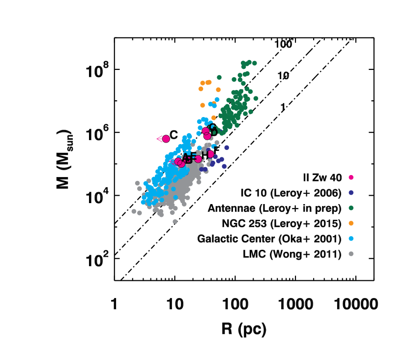
Figure 15.— CO-derived mass as a function of radius for  and the comparison sample. The dashed-dotted lines indicated lines of constant mass surface density (100, 10, 1 $\rm M_{\odot}pc^{-2}$). When the proper $\alpha_{co}$ conversion factor is used, the clouds in  have similar mass surface densities to those in the Galactic Center, the Antennae, and NGC 253 and on the upper end of those in IC 10 and the LMC. Therefore, the low CO surface brightnesses in  are due to the lower $\alpha_{co}$ value in this galaxy, not clouds with intrinsically low mass surface densities.

To explore the trend of mass surface density with metallicity further, we plot the CO surface brightness as a function of metallicity in the left panel of Figure 16. For this plot, we have selected comparison galaxies with CO observations at comparable spatial resolution ($\sim 30$pc) with a range of metallicities including the Milky Way (Heyer et al., 2009), the LMC (Wong et al., 2011), IC 10 (Leroy et al., 2006), NGC 1569, NGC 205, and SMC (Bolatto et al., 2008), M31 (Scruba et al. in prep), M33 (Rosolowsky et al., 2007), the Antennae (Whitmore et al., 2014, ; Leroy et al. in prep), and NGC 253 (Leroy et al., 2015). As expected, we find that the CO surface brightness for galaxies with metallicities less than 12+log(O/H)=8.6 is less than or equal to 10 $\rm{K\,km\,s^{-1}}$. However, when the proper $\alpha_{co}$ values are applied to the data, we find that at least two of the galaxies (II Zw 40 and the LMC) have larger mass surface densities than expected if we applied a Galactic $\alpha_{co}$ value to a CO surface brightness limit of 10$\rm{K\,km\,s^{-1}}$. This result shows that the low CO surface brightnesses seen in low metallicity galaxies do not necessarily mean that the molecular gas surface densities in these galaxies are low.

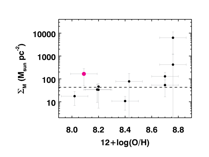
Figure 16.— CO surface brightness (left) and mass surface density (right) of clouds as a function of metallicity for  (magenta point) and galaxies with CO observations at comparable spatial resolutions ($\sim 30$pc). The CO surface brightnesses for galaxies with metallicities less than 12+log(O/H)=8.6 are less than or equal to 10 $\rm{K\,km\,s^{-1}}$(dashed line). However, when the appropriate $\alpha_{co}$ values are applied to the data, the molecular surface densities in two of our low metallicity galaxies ( and the LMC) exceed the expected 10 $\rm{K\,km\,s^{-1}}$ mass surface density for a Galactic $\alpha_{co}$ value. Therefore, the low CO surface brightnesses found in low metallicity systems does not necessarily imply that these systems have low molecular gas mass surface densities.

III.2.5 The Size-Linewidth Relationship

The last fundamental molecular cloud relationship we will investigate is the size-linewidth relationship, which is thought to arise from the turbulent cascade of energy within a molecular cloud. The location of clouds within this plot reflects the combined effects of virial equilibrium, turbulence, and external pressure. For viralized clouds, the normalization of this relationship is set by cloud surface density. As we saw in § III.2.4, the surface brightnesses of clouds in the Milky Way (Solomon et al., 1987; Heyer et al., 2009) and in high resolution studies of nearby galaxies (Wong et al., 2011; Bolatto et al., 2008) are similar and thus their clouds fall along the same size-linewidth relationship. Higher surface densities clouds like those seen in the nuclear starburst NGC 253 (Leroy et al., 2015) and in the Antennae (Whitmore et al., 2014, Leroy et al. in prep) have higher normalization factors due to their high gas surface densities. Finally, clouds can be elevated beyond the nominal normalization factor derived from their surface densities by higher external pressures, such as those found in the center of the Milky Way (Oka et al., 2001).

Figure 17 compares the sizes and linewidths of clouds within  to those in our comparison samples. We find that the molecular clouds within  have larger than average linewidths for their size compared to clouds in the Milky Way, suggesting that external pressure and/or high gas surface densities play a significant role in shaping the molecular clouds within this galaxy. We note that IC 10, one of the few other dwarf starbursts with measured molecular cloud properties, displays similar properties to , but that clouds in the LMC generally have smaller linewidths compared to those in . Deep neutral hydrogen observations suggest that IC 10 is either an advanced merger or has an infalling gas cloud (Ashley et al., 2014). The molecular clouds in this galaxy also lie largely on the edges of super-shells produced by stellar winds and supernovae generated by its on-going burst of star formation (Leroy et al., 2006).

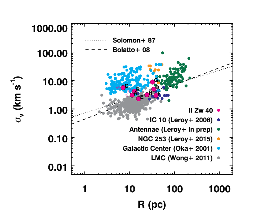
Figure 17.— The size-linewidth relationship for molecular clouds within  and our comparison galaxies. The clouds in  are shown as magenta circles outlined in black and labeled. The points show different comparison samples of clouds including: the Large Magellanic Cloud (gray points; Wong et al., 2011), the Local Group dwarf starburst IC 10 (purple points; Leroy et al., 2006), the massive late-stage merger referred to as the Antennae (dark green points; Whitmore et al., 2014, Leroy et al., in prep), the nuclear starburst NGC 253 (orange points; Leroy et al., 2015), and the center of the Milky Way (cyan points; Oka et al., 2001). The lines show the fiducial size-linewidth relationships from Solomon et al. (1987) (dotted) and Bolatto et al. (2008) (dashed). The clouds within  lie above the fiducial size-linewidth relationship seen in the Milky Way and the relationship seen in the LMC and have similar velocities for their size to clouds in the Galactic Center, the Antennae, and the dwarf starburst IC 10. This trend suggests that either external pressure or turbulence play a key role in driving the linewidths of the clouds within .

To further distinguish between the different samples, we compare the distribution of the square of the coefficient of the size-linewidth relationship ($C^{2}=\sigma_{v}^{2}/R$), which is proportional to the molecular gas surface density if the cloud is in virial equilibrium, in the different samples (Figure 18). This plot makes clear that the  clouds have the largest overlap with the clouds seen in the Antennae, although they do also overlap the upper end of the Milky Way molecular clouds and the lower end of the molecular clouds in NGC 253 and the Inner Galaxy. Again, the clouds in  and the nearby dwarf starburst galaxy IC 10 have similar values. This result suggests that the clouds in  have higher surface densities than found in the disk of the Milky Way (if they are in virial equilibrium).

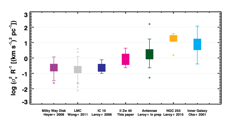
Figure 18.— Distribution of the coefficient of the size-linewidth relationship squared ($\sigma_{V}^{2}/R$), which is proportional to the GMC surface density in virial equilibrium, for  and comparison sample. The lower and upper ends of the box demarcate the first and fourth quartile. The whiskers at the tops of the box extend to the minimum and maximum of the distribution or 1.5 times the mininum or maximum. Outliers are shown as circles. Although all samples have a wide range of values, the size-linewidth coefficients in  are most similar to those seen in the Antennae. Like , the Antennae are undergoing a major merger between two galaxies, although for the Antennae the progenitor galaxies are more massive than the dwarf progenitors involved in the  merger. The size-linewidth coefficients for the nuclear starburst NGC 253 and the center of the Milky Way are, in general, larger than the coefficients for either the Antennae or . The distribution of size-linewidth points in IC 10, a dwarf starburst galaxy in the Local Group, is similar, although not quite as high as that for . IC 10 shows signs of large-scale gas shocks. The neutral hydrogen distribution of IC 10 is consistent with either late-stage merger or an infalling gas cloud (Ashley et al., 2014) and the molecular gas lies on the edges of the super-shells created by the on-going burst of star formation in this galaxy (Leroy et al., 2006).

To investigate whether high external pressures may be playing a role in , we compare the size-linewidth coefficient squared to the surface density of the molecular gas determined using CO in Figure 19. Clouds in virial equilibrium will fall along the solid line in this diagram, while clouds requiring high external pressures will fall above the line. The dashed lines indicate the required external pressure to maintain virial equilibrium. However, since we have assumed virial equlibrium to determine $\alpha_{co}$ (see III.2.2), our clouds will fall along the virial equilibrium line by design.

To show the effects of different $\alpha_{co}$ assumptions, we include in Figure 19 points using our CO-based $\alpha_{co}$ measurements (large magenta points) as well as a Milky Way $\alpha_{co}$ value and the dust-based $\alpha_{co}$ estimate derived in III.2.2 (small magenta points to the left and right of the virial equilibrium line, respectively). Using a Milky Way $\alpha_{co}$ value would imply that our clouds require external pressures ranging over two orders of magnitude from $10^{4}\ \rm{K\,cm^{-3}}$ to $10^{6}\ \rm{K\,cm^{-3}}$, while a dust-based $\alpha_{co}$ estimate would imply that all of our clouds are sub-virial and collapsing. Although these effects could arise in strong turbulent flows, we argue that the more likely origin of the large linewidths with  is high surface densities generated by the large scale gas shocks driven by its on-going merger since our CO-derived $\alpha_{co}$ factor is consistent with CO-based measurements of $\alpha_{co}$ in other galaxies with similar metallicity (see § III.2.2). Given this, we do not find any strong evidence that the clouds within  require high external pressures to maintain their large linewidths.

The two clouds with the greatest deviations from the size-linewidth relationship – clouds C and G – occupy interesting regions of this diagram. Cloud C lies below the virial equilibrium line even with using our adopted $\alpha_{co}$ value. This cloud appears to have already collapsed and formed multiple young massive clusters. High resolution radio continuum images find at least three embedded sources with ionizing photon fluxes comparable to 30 Doradus – the closest example of a starburst – associated with cloud C (Kepley et al., 2014). The optical cluster near cloud C has an age of less than 5Myr, which supports the idea that cloud C recently collapsed. Cloud G, which also has line ratios consistent with colder CO, would require the highest external pressures ($10^{6}\ \rm{K\,cm^{-3}}$) to maintain virial equilibrium, suggesting that it could be a progenitor of a super star cluster (Johnson et al., 2015).

A related key parameter for quantifying the clouds within  is the turbulent Mach number (Leroy et al., 2015):

$$\mathcal{M}=\sqrt{3}\sigma_{1d}/c_{s}$$ (4)

where $\sigma_{1d}$ is the one dimensional velocity dispersion and $c_{s}$ is the sound speed. We adopt a value of 0.2 $\rm{km\,s}^{-1}$ for $c_{s}$, which assumes an isothermal molecular gas with a temperature of 10K. We note that the gas temperature may be higher closer to the star-forming region. The value used here reflects the average temperature of the molecular clouds throughout the central region. The median Mach number of clouds in  is $\sim 36$ with values ranging from 20 to 76. Comparing these values with those for giant molecular clouds in the Milky Way and in NGC 253 (see Table 4 in Leroy et al., 2015), we find that the median Mach number within  is higher than that found in molecular clouds in the Milky Way disk (11), but below that of the clouds in the nuclear starburst galaxy NGC 253 (85). The Mach number within  is consistent with the increased Mach numbers necessary to produce virialized clouds.

Overall, these results suggest that the large-scale gas shocks due to ’s on-going merger are driving high molecular gas surface densities in , leading to elevated linewidths. We caution that  is clearly a rapidly evolving system. It is possible that some (or all) of the molecular gas structures we see here are transient, unbound features that will not collapse to form stars. However, our estimates of $\alpha_{co}$ are consistent with other virial equilibrium based estimates of this value at low metallicity (see § III.2.2 for a discussion), which suggests that the  clouds identified here are most likely bound objects.

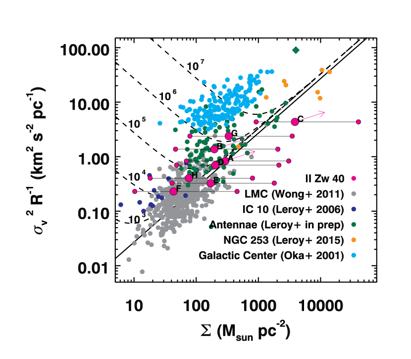
Figure 19.— The coefficient of the size-linewidth relationship squared ($\sigma_{V}^{2}/R$) as a function of molecular gas surface density derived from CO observations for molecular clouds within  and our sample of comparison galaxies. Clouds on the solid line are in virial equilibrium, while clouds above the line require external pressures to maintain equilibrium. The dotted lines indicate the required external pressures in units of $\rm{K\,cm^{-3}}$. The clouds in  are shown as magenta circles outlined in black. The large magenta circles use our CO-based $\alpha_{co}$ measurement (see § III.2.2), while the small circles on the left side of the diagram use a Milky Way estimate (4.3$\rm M_{\odot}(\rm K\,\rm{km\,s}^{-1}\,pc^{2})^{-1}$) and those on the right side of the diagram use our dust-derived $\alpha_{co}$ estimate (see III.2.2). The points show different comparison samples of clouds including: the Large Magellanic Cloud (gray points; Wong et al., 2011), the Local Group dwarf starburst IC 10 (purple points; Leroy et al., 2006), the massive late-stage merger referred to as the Antennae (dark green points; Leroy et al., in prep) with the candidate super star cluster progenitor referred to as the Firecracker (Johnson et al., 2015) shown as a dark green diamond, the nuclear starburst NGC 253 (orange points; Leroy et al., 2015), and the center of the Milky Way (cyan points; Oka et al., 2001). The  clouds will lie on the virial equilibrium line in this diagram because we have assumed virial equilibrium to derive the $\alpha_{co}$ value. However, we argue that the CO-based $\alpha_{co}$ value used here is approximately correct because it agrees with $\alpha_{co}$ values determined in other systems with similar metallicities. Adopting a Milky Way $\alpha_{co}$ factor would require that the clouds be confined by external pressures ranging from $10^{4}\ \rm{K\,cm^{-3}}$ to $10^{6}\ \rm{K\,cm^{-3}}$, while adopting a dust-based $\alpha_{co}$ estimate would imply that all of our clouds are sub-virial and collapsing. Thus, the large linewidths in  appear to be the result of the high gas surface densities due to ’s on-going merger and not large external pressures.

IV. Summary and Conclusions

In this paper, we present high-resolution ($\sim 24$ pc) ALMA observations of $\rm{{}^{12}CO({3}-{2})}$ and $\rm{{}^{12}CO({2}-{1})}$ emission and 3 mm, 1 mm, and 870µm continuum emission in the prototypical blue compact dwarf galaxy . Our goal is to characterize the molecular gas content within this unique, low metallicity and high star formation rate surface density environment and compare it to the molecular clouds properties seen in other environments to gain insight into the fundamental physical processes driving star formation in galaxies.

Due to the combination of relatively bright line emission and excellent surface brightness sensitivity, our highest signal-to-noise CO detection is $\rm{{}^{12}CO({3}-{2})}$ in ALMA Band 7. The distribution of the CO emission tracing the molecular clouds and various star formation tracers is consistent with a picture of merger-driven star formation within . The CO emission within this galaxy is clumpy and distributed throughout the central star-forming region of  and its kinematics are similar, but not identical to, that of the galaxy’s neutral hydrogen reservoir. Only one of the molecular clouds traced by the CO emission has associated star formation, suggesting that the other clouds, in particular the relatively cold cloud G, will serve as future sites for star formation or are transient molecular features.

The centimeter through submillimeter continuum spectral energy distribution of  is dominated by free-free and synchrotron emission. Dust emission only begins to play a role at 1 mm and is only 50% of the total emission at 870µm. We derive a total dust mass of $1.4\times 10^{4}\ \rm{M}_{\odot}$ and a gas-to-dust ratio of between 770 and 3500. The lower end of this range is consistent with other estimates based on far-infrared data. The gas-to-dust ratio derived here may be an overestimate if we have resolved out significant continuum emission.

Using the high spatial resolution provided by ALMA, we have used the $\rm{{}^{12}CO({3}-{2})}$ data to measure the giant molecular cloud sizes, line widths, and luminosities within  and compared their properties with populations of clouds in other fiducial star-forming environments including the Galactic Center (Oka et al., 2001), the Large Magellanic Cloud (Wong et al., 2011), the Local Group low metallicity irregular IC 10 (Leroy et al., 2006), the nuclear starburst NGC 253 (Leroy et al., 2015), and the merging Antennae system (Whitmore et al., 2014, Leroy et al. in prep).

Using our CO and continuum data, we find that the CO-to-H₂ conversion factor in  is at least four times higher than in the Milky Way (18.1 $\rm M_{\odot}(\rm K\,\rm{km\,s}^{-1}\,pc^{2})^{-1}$) and may be as much as 35 times higher (150 $\rm M_{\odot}(\rm K\,\rm{km\,s}^{-1}\,pc^{2})^{-1}$). The lower limit is based on an average virial equilibrium estimate for the resolved clouds in . This value is comparable to CO-based virial equilibrium measurements in other low metallicity galaxies. The upper limit is based on a new method that uses simple photodissociation models by Wolfire et al. (2010) and the resolved line intensity to uniquely predict $\alpha_{co}$. We note that the CO-to-H₂ conversion factors based on the numerical models of Narayanan et al. (2012) may underestimate the conversion factor, especially in low metallicity systems.

We use the derived conversion factor to estimate the molecular star formation efficiency of . We find that even using our largest estimate of the CO-to-H₂ conversion factor the molecular star formation efficiency of  is still larger than the typical value by a factor of 10. This high value could be due to truly high molecular star formation efficiencies in these systems, or more likely, time-dependent evolutionary effects due to ’s on-going merger. We also find that the low CO surface brightnesses in  and other low metallicity galaxies from the literature do not necessarily imply that these systems have low molecular gas surface densities. The low CO surface brightness in these galaxies appears to be due to reduced dust shielding for CO, not to intrinsically low surface density molecular gas.

The properties of the clouds within  reveal that the large-scale gas shocks produced by its on-going merger and subsequent star formation may play a key role in shaping the molecular clouds. On average, the clouds in  lie above the Milky Way size-linewidth relationship and have higher size linewidth coefficients. Their size-linewidths coefficients, which are proportional to the virial mass surface densities, are comparable to those found the Antennae, which is a late-stage merger, and IC 10, whose neutral hydrogen distribution is consistent with either an advanced merger or an infalling gas cloud and whose molecular gas lies on the edges of large-scale shells due to on-going star formation. They are lower than those in the nuclear starburst NGC 253 or the Galactic Center. Increased surface densities leading to higher linewidths appear to the origin of the elevated size-linewidth coefficients in , rather than large external pressures. We note that this result does depend on the adopted $\alpha_{co}$ value.

Using  as a template, we can extend our results to make several inferences about properties of molecular gas in blue compact dwarfs. First, the properties of the molecular gas in  are driven by the large-scale gas shocks induced by its on-going merger, not by its metallicity. The low metallicity of this galaxy only affects the observability of the most commonly used molecular gas tracer CO.  is not a unique case; many blue compact dwarf galaxies appear to be the result of mergers or interactions (Martínez-Delgado et al., 2012; Lelli et al., 2014; Stierwalt et al., 2015). Indeed, unresolved, single-dish $\rm{{}^{12}CO({3}-{2})}$ and $\rm{{}^{12}CO({1}-{0})}$ observations of a sample of eight dwarf starburst galaxies have also found that the line ratios and derived densities and temperatures of the molecular gas in their sample have more in common with that of starburst galaxies than of low metallicity galaxies (Meier et al., 2001).

Second, as  shows, the star formation histories of blue compact dwarfs are complex and vary rapidly with time, unlike larger spiral galaxies which more or less continuously form stars at a low rate. In other words, blue compact dwarfs are more like firecrackers than the slow-burning bonfires of spiral galaxies. Therefore, comparing present day gas content to current star formation to derive molecular star formation efficiencies and other related quantities in blue compact dwarfs is misleading at best. The high molecular gas star formation efficiencies seen here in  and claimed for other galaxies (Turner et al., 2015) are likely the result of the massive burst of star formation – which establishes a source as a blue compact dwarf galaxy – using up a majority of the molecular gas in a galaxy. Building up larger samples of molecular gas in dwarf galaxies in different evolutionary stages – now possible with the power of ALMA – is key to understanding the properties of their molecular gas and star formation in these sources.

Based on our results, we suggest two avenues for future studies of the molecular gas in these unique systems. First, CO detection experiments for low-metallicity galaxies like  should focus on the $\rm{{}^{12}CO({2}-{1})}$ or $\rm{{}^{12}CO({3}-{2})}$ transitions, which are significantly brighter than the ground state transition. In particular for ALMA, Band 7 observations of $\rm{{}^{12}CO({3}-{2})}$ should have the highest signal-to-noise, assuming that other blue compact dwarf galaxies have similar CO excitations.

Second, although the sensitivity and resolution of ALMA allow us to extend detailed CO studies to galaxies like , the use of other molecular gas tracers in these galaxies needs to be explored. One commonly used tracer of molecular gas is dust continuum emission. Although this is a powerful tracer, as we have demonstrated here, the dust emission in these galaxies is faint even at 870µm and blended with free-free emission. Higher resolution ($\sim 1\arcsec$) far-infared and neutral hydrogen observations would be another way to probe the molecular gas content of these galaxies, but require the development of a high resolution far-infrared telescope and something like the Square Kilometer Array (SKA). Another promising tracer might be CI (Glover & Clark, 2015b) or CII (Glover & Clark, 2015a), which may be prevalent throughout molecular cloud envelope, but may also extend beyond the cloud.

Appendix A Derivation of Predicted CO-to-H₂ Conversion Factor as a Function of Metallicity and Integrated CO Line Intensity

In the Wolfire et al. (2010) models of the dark molecular gas, the estimated CO-to-H₂ conversion factor depends strongly on the average extinction through the giant molecular cloud, which is turn depends on both the metallicity of the system and the column density of the giant molecular cloud. For extragalactic observations that do not resolve molecular clouds, the column density must be assumed and is commonly set to values similar to those found in Milky Way clouds. For resolved observations like those presented in this paper, the observed CO brightness of the cloud adds an additional constraint

$$\bar{N}_{22}={\rm X_{CO}}(Z)W_{CO}/(1\times 10^{22}cm^{-2})$$ (A1)

where $W_{CO}$ has units of $\rm{K\,km\,s^{-1}}$and ${\rm X_{CO}}$ has units of ${\rm cm}^{-2}\,({\rm K}\,\rm{km\,s}^{-1})^{-1}$. Thus, in the resolved case, the estimated CO-to-H₂ conversion factor depends both on the metallicity, the CO line intensities, and itself. In this appendix, we solve for the estimated CO-to-H₂ conversion factor as a function of metallicity and CO line intensity.

Following Wolfire et al. (2010), Bolatto et al. (2013) derive the following relationship between the mean extinction through a cloud and value of $\alpha_{co}$ relative to the value at solar metallicity

$$\frac{{\rm X_{CO}}\ (Z^{\prime})}{{\rm X_{CO}}\ (Z^{\prime}=1)}=\exp{\left[\left(\frac{4.0\Delta A_{V}}{\bar{A}_{V,MW}}\right)\left(\frac{1-Z^{\prime}}{Z^{\prime}}\right)\right]}$$ (A2)

where $Z^{\prime}$ is the metallicity of the galaxy relative to solar, ${\rm X_{CO}}(Z^{\prime})$ is the value of ${\rm X_{CO}}$ at metallicity $Z^{\prime}$, ${\rm X_{CO}}(Z^{\prime}=1)$ is the value of ${\rm X_{CO}}$ at solar metallicity ($2\times 10^{-2}\ {\rm cm}^{-2}\,({\rm K}\,\rm{km\,s}^{-1})^{-1}$; Bolatto et al., 2013), $\Delta A_{v}$ difference in extinction between the CO-dark layer of gas and the CO-emitting layer, and $\bar{A}_{V,MW}$ is the mean extinction through the giant molecular cloud. The mean extinction through the giant molecular cloud is given by the expression

$$\bar{A}_{V}=5.26\,\delta_{DGR}^{\prime}\,\bar{N}_{22}$$ (A3)

where $\delta_{DGR}^{\prime}$ is the dust-to-gas ratio relative to the local Galactic value and $\bar{N}_{22}$ is the mean hydrogen column density of the cloud in units of $10^{22}\,\rm{cm}^{-2}$. For $\bar{A}_{V,MW}$, the quantity $\delta_{DGR}^{\prime}$ equals one. Substituting Equations (A1) and (A3) into Equation (A2), we obtain

$$\frac{{\rm X_{CO}}\ (Z^{\prime})}{{\rm X_{CO}}\ (Z^{\prime}=1)}=\exp{\left[\left(\frac{{\rm X_{CO}}(Z^{\prime}=1)}{{\rm X_{CO}}(Z^{\prime})}\right)\left(\frac{7.604\times 10^{21}\Delta A_{V}}{W_{CO}{\rm X_{CO}}(Z^{\prime}=1)}\right)\left(\frac{1-Z^{\prime}}{Z^{\prime}}\right)\right]},$$ (A4)

which we rearrange to obtain

$$\frac{{\rm X_{CO}}(Z^{\prime})}{{\rm X_{CO}}(Z^{\prime}=1)}\ln{\left(\frac{{\rm X_{CO}}(Z^{\prime})}{{\rm X_{CO}}(Z^{\prime}=1)}\right)}=\left(\frac{7.604\times 10^{21}\Delta A_{V}}{W_{CO}{\rm X_{CO}}(Z^{\prime}=1)}\right)\left(\frac{1-Z^{\prime}}{Z^{\prime}}\right).$$ (A5)

We use Equation (A5) to calculate how the value of ${\rm X_{CO}}$ changes with the $W_{CO}$ and $Z^{\prime}$. The term $\Delta A_{V}$ has only a weak dependence on metallicity, so we adopt the mean value for $\Delta A_{V}$ from (Wolfire et al., 2010): 0.7. The solution to this equation is of the form

$$x=\exp{(W(c))}$$ (A6)

where $W(c)$ is the Lambert W function, $x$ is ${\rm X_{CO}}(Z^{\prime})/{\rm X_{CO}}(Z^{\prime}=1)$, and $c$ is the right hand size of Equation (A5). The value for the ${\rm X_{CO}}$ ratio is plotted in Figure 20 as a function of integrated line intensity ($W_{CO}$) and metallicity ($Z^{\prime}$).

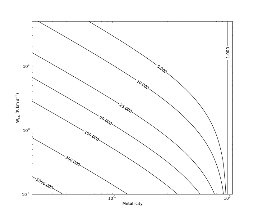
Figure 20.— The ratio ${\rm X_{CO}}(Z^{\prime})/{\rm X_{CO}}(Z^{\prime}=1)$ as a function of integrated line intensity ($W_{CO}$) and metallicity relative to solar ($Z^{\prime}$). This calculation takes into account the strong dependence of the fraction of dark molecular gas on the column density of the molecular gas.

Table 6Properties of Giant Molecular Clouds Within

	RA	Dec	V	$L_{CO(3-2)}$			$L_{CO(2-1)}$			$L_{CO(1-0)}$			$\sigma_{v}$	$R$	$M_{v}$	$T_{b}(3-2)$	$T_{b}(2-1)$
Label	J2000	J2000	$\rm{km\,s}^{-1}$	$\rm K\,\rm{km\,s}^{-1}\,pc^{2}$			$\rm K\,\rm{km\,s}^{-1}\,pc^{2}$			$\rm K\,\rm{km\,s}^{-1}\,pc^{2}$			$\rm{km\,s}^{-1}$	pc	$10^{5}M_{\odot}$	K	K
(1)	(2)	(3)	(4)	(5)			(6)			(7)			(8)	(9)	(10)	(11)	(12)
A	5:55:42.268	3:23:27.45	769.0	3600	$\pm$	400	1100	$\pm$	200	6600	$\pm$	3400	3.08 $\pm$ 0.02	$<$11.4	$<$1.1	0.9	1.0
B	5:55:42.572	3:23:31.57	738.5	3000	$\pm$	300	1900	$\pm$	400	5600	$\pm$	2900	4.19 $\pm$ 0.04	$<$12.8	$<$2.3	0.5	0.8
C	5:55:42.620	3:23:32.13	754.7	18700	$\pm$	2000	18300	$\pm$	3700	34500	$\pm$	17600	5.58 $\pm$ 0.07	$<$7.2	$<$2.3	1.3	2.5
D	5:55:42.654	3:23:32.30	746.1	22900	$\pm$	2400	39500	$\pm$	7900	42200	$\pm$	21500	4.92 $\pm$ 0.05	34.6 $\pm$ 1.2	4.6 $\pm$ 0.2	1.4	2.8
E	5:55:42.733	3:23:30.18	742.1	4100	$\pm$	400	2900	$\pm$	600	7500	$\pm$	3800	2.28 $\pm$ 0.02	15.9 $\pm$ 3.8	0.4 $\pm$ 0.1	0.7	1.5
F	5:55:42.790	3:23:33.56	730.1	6100	$\pm$	600	4600	$\pm$	900	11300	$\pm$	5800	2.99 $\pm$ 0.03	38.8 $\pm$ 0.7	1.9 $\pm$ 0.1	0.7	1.1
G	5:55:42.808	3:23:32.61	763.8	20700	$\pm$	2100	26900	$\pm$	5400	60900	$\pm$	31100	8.79 $\pm$ 0.04	32.5 $\pm$ 0.5	13.7 $\pm$ 0.3	0.9	2.2
H	5:55:42.891	3:23:32.03	761.4	4300	$\pm$	400	3000	$\pm$	600	7900	$\pm$	4000	3.13 $\pm$ 0.03	24.4 $\pm$ 0.9	1.3 $\pm$ 0.1	0.7	1.2

Note. — Column (1): Cloud label. Columns (2) and (3): Right Ascension and Declination of the luminosity weighted center of the cloud in J2000. Column (4): Mean luminosity-weighted velocity of cloud in the LSRK frame. Column (5): Measured $\rm{{}^{12}CO({3}-{2})}$ luminosity. Column (6): Measured $\rm{{}^{12}CO({2}-{1})}$ luminosity. Column (7): Estimate of $\rm{{}^{12}CO({1}-{0})}$ luminosity based on observed $\rm{{}^{12}CO({3}-{2})}$ luminosity and ${\rm r_{31}}$ ratio (see §III.2.1 for details). Column (8): Linewidth of cloud derived using $\rm{{}^{12}CO({3}-{2})}$ data. Column (9): Size of cloud derived using $\rm{{}^{12}CO({3}-{2})}$ data. (see §III.2.1 for details). Column (10): Virial mass of cloud derived using $\rm{{}^{12}CO({3}-{2})}$ data (see §III.2.1 for details). Column (11) and Column (12): Peak $\rm{{}^{12}CO({3}-{2})}$ and $\rm{{}^{12}CO({2}-{1})}$ temperature of the cloud.

References

- Albrecht et al. (2004) Albrecht, M., Chini, R., Krügel, E., Müller, S. A. H., & Lemke, R. 2004, A&A, 414, 141
- Ashley et al. (2014) Ashley, T., Elmegreen, B. G., Johnson, M., Nidever, D. L., Simpson, C. E., & Pokhrel, N. R. 2014, AJ, 148, 130
- Baldwin et al. (1982) Baldwin, J. A., Spinrad, H., & Terlevich, R. 1982, MNRAS, 198, 535
- Bolatto et al. (2008) Bolatto, A. D., Leroy, A. K., Rosolowsky, E., Walter, F., & Blitz, L. 2008, ApJ, 686, 948
- Bolatto et al. (2013) Bolatto, A. D., Wolfire, M., & Leroy, A. K. 2013, ARA&A, 51, 207
- Brinks & Klein (1988) Brinks, E., & Klein, U. 1988, MNRAS, 231, 63P
- Cardamone et al. (2009) Cardamone, C., Schawinski, K., Sarzi, M., Bamford, S. P., Bennert, N., Urry, C. M., Lintott, C., Keel, W. C., Parejko, J., Nichol, R. C., Thomas, D., Andreescu, D., Murray, P., Raddick, M. J., Slosar, A., Szalay, A., & Vandenberg, J. 2009, MNRAS, 399, 1191
- Chen et al. (2010) Chen, C.-H. R., Indebetouw, R., Chu, Y.-H., Gruendl, R. A., Testor, G., Heitsch, F., Seale, J. P., Meixner, M., & Sewilo, M. 2010, ApJ, 721, 1206
- Daddi et al. (2010) Daddi, E., Elbaz, D., Walter, F., Bournaud, F., Salmi, F., Carilli, C., Dannerbauer, H., Dickinson, M., Monaco, P., & Riechers, D. 2010, ApJ, 714, L118
- Fomalont et al. (2014) Fomalont, E., van Kempen, T., Kneissl, R., Marcelino, N., Barkats, D., Corder, S., Cortes, P., Hills, R., Lucas, R., Manning, A., & Peck, A. 2014, The Messenger, 155, 19
- Gil de Paz et al. (2003) Gil de Paz, A., Madore, B. F., & Pevunova, O. 2003, ApJS, 147, 29
- Glover & Clark (2012) Glover, S. C. O., & Clark, P. C. 2012, MNRAS, 421, 9
- Glover & Clark (2015a) —. 2015a, ArXiv e-prints
- Glover & Clark (2015b) —. 2015b, ArXiv e-prints
- Grocholski et al. (2008) Grocholski, A. J., Aloisi, A., van der Marel, R. P., Mack, J., Annibali, F., Angeretti, L., Greggio, L., Held, E. V., Romano, D., Sirianni, M., & Tosi, M. 2008, ApJ, 686, L79
- Guseva et al. (2000) Guseva, N. G., Izotov, Y. I., & Thuan, T. X. 2000, ApJ, 531, 776
- Heiderman et al. (2010) Heiderman, A., Evans, II, N. J., Allen, L. E., Huard, T., & Heyer, M. 2010, ApJ, 723, 1019
- Heyer et al. (2009) Heyer, M., Krawczyk, C., Duval, J., & Jackson, J. M. 2009, ApJ, 699, 1092
- Hibbard & Mihos (1995) Hibbard, J. E., & Mihos, J. C. 1995, AJ, 110, 140
- Hughes et al. (2013) Hughes, A., Meidt, S. E., Colombo, D., Schinnerer, E., Pety, J., Leroy, A. K., Dobbs, C. L., García-Burillo, S., Thompson, T. A., Dumas, G., Schuster, K. F., & Kramer, C. 2013, ApJ, 779, 46
- Hunt et al. (2014) Hunt, L. K., Testi, L., Casasola, V., García-Burillo, S., Combes, F., Nikutta, R., Caselli, P., Henkel, C., Maiolino, R., Menten, K. M., Sauvage, M., & Weiss, A. 2014, A&A, 561, A49
- Hunter et al. (2000) Hunter, D. A., O’Connell, R. W., Gallagher, J. S., & Smecker-Hane, T. A. 2000, AJ, 120, 2383
- Inoue (2001) Inoue, A. K. 2001, AJ, 122, 1788
- Israel (1997) Israel, F. P. 1997, A&A, 328, 471
- Izotov et al. (2011) Izotov, Y. I., Guseva, N. G., & Thuan, T. X. 2011, ApJ, 728, 161
- Johnson et al. (2015) Johnson, K. E., Leroy, A. K., Indebetouw, R., Brogan, C. L., Whitmore, B. C., Hibbard, J., Sheth, K., & Evans, A. S. 2015, ApJ, 806, 35
- Karl et al. (2010) Karl, S. J., Naab, T., Johansson, P. H., Kotarba, H., Boily, C. M., Renaud, F., & Theis, C. 2010, ApJ, 715, L88
- Kawamura et al. (2009) Kawamura, A., Mizuno, Y., Minamidani, T., Filipović, M. D., Staveley-Smith, L., Kim, S., Mizuno, N., Onishi, T., Mizuno, A., & Fukui, Y. 2009, ApJS, 184, 1
- Kennicutt (1998) Kennicutt, Jr., R. C. 1998, ApJ, 498, 541
- Kepley et al. (2014) Kepley, A. A., Reines, A. E., Johnson, K. E., & Walker, L. M. 2014, AJ, 147, 43
- Keto et al. (2005) Keto, E., Ho, L. C., & Lo, K.-Y. 2005, ApJ, 635, 1062
- Klein et al. (1991) Klein, U., Weiland, H., & Brinks, E. 1991, A&A, 246, 323
- Krumholz (2012) Krumholz, M. R. 2012, ApJ, 759, 9
- Krumholz et al. (2006) Krumholz, M. R., Matzner, C. D., & McKee, C. F. 2006, ApJ, 653, 361
- Larson (1981) Larson, R. B. 1981, MNRAS, 194, 809
- Leech et al. (2010) Leech, J., Isaak, K. G., Papadopoulos, P. P., Gao, Y., & Davis, G. R. 2010, MNRAS, 406, 1364
- Lelli et al. (2014) Lelli, F., Verheijen, M., & Fraternali, F. 2014, MNRAS, 445, 1694
- Leroy et al. (2006) Leroy, A., Bolatto, A., Walter, F., & Blitz, L. 2006, ApJ, 643, 825
- Leroy et al. (2012) Leroy, A. K., Bigiel, F., de Blok, W. J. G., Boissier, S., Bolatto, A., Brinks, E., Madore, B., Munoz-Mateos, J.-C., Murphy, E., Sandstrom, K., Schruba, A., & Walter, F. 2012, AJ, 144, 3
- Leroy et al. (2011) Leroy, A. K., Bolatto, A., Gordon, K., Sandstrom, K., Gratier, P., Rosolowsky, E., Engelbracht, C. W., Mizuno, N., Corbelli, E., Fukui, Y., & Kawamura, A. 2011, ApJ, 737, 12
- Leroy et al. (2015) Leroy, A. K., Bolatto, A. D., Ostriker, E. C., Rosolowsky, E., Walter, F., Warren, S. R., Donovan Meyer, J., Hodge, J., Meier, D. S., Ott, J., Sandstrom, K., Schruba, A., Veilleux, S., & Zwaan, M. 2015, ApJ, 801, 25
- Leroy et al. (2008) Leroy, A. K., Walter, F., Brinks, E., Bigiel, F., de Blok, W. J. G., Madore, B., & Thornley, M. D. 2008, AJ, 136, 2782
- Leroy et al. (2013) Leroy, A. K., Walter, F., Sandstrom, K., Schruba, A., Munoz-Mateos, J.-C., Bigiel, F., Bolatto, A., Brinks, E., de Blok, W. J. G., Meidt, S., Rix, H.-W., Rosolowsky, E., Schinnerer, E., Schuster, K.-F., & Usero, A. 2013, AJ, 146, 19
- Madden et al. (2006) Madden, S. C., Galliano, F., Jones, A. P., & Sauvage, M. 2006, A&A, 446, 877
- Mao et al. (2010) Mao, R.-Q., Schulz, A., Henkel, C., Mauersberger, R., Muders, D., & Dinh-V-Trung. 2010, ApJ, 724, 1336
- Martínez-Delgado et al. (2012) Martínez-Delgado, D., Romanowsky, A. J., Gabany, R. J., Annibali, F., Arnold, J. A., Fliri, J., Zibetti, S., van der Marel, R. P., Rix, H.-W., Chonis, T. S., Carballo-Bello, J. A., Aloisi, A., Macciò, A. V., Gallego-Laborda, J., Brodie, J. P., & Merrifield, M. R. 2012, ApJ, 748, L24
- Mauersberger et al. (1999) Mauersberger, R., Henkel, C., Walsh, W., & Schulz, A. 1999, A&A, 341, 256
- McKee & Krumholz (2010) McKee, C. F., & Krumholz, M. R. 2010, ApJ, 709, 308
- McMullin et al. (2007) McMullin, J. P., Waters, B., Schiebel, D., Young, W., & Golap, K. 2007, in Astronomical Society of the Pacific Conference Series, Vol. 376, Astronomical Data Analysis Software and Systems XVI, ed. R. A. Shaw, F. Hill, & D. J. Bell, 127
- Meier et al. (2001) Meier, D. S., Turner, J. L., Crosthwaite, L. P., & Beck, S. C. 2001, AJ, 121, 740
- Murphy et al. (2012) Murphy, E. J., Bremseth, J., Mason, B. S., Condon, J. J., Schinnerer, E., Aniano, G., Armus, L., Helou, G., Turner, J. L., & Jarrett, T. H. 2012, ApJ, 761, 97
- Murphy et al. (2011) Murphy, E. J., Condon, J. J., Schinnerer, E., Kennicutt, R. C., Calzetti, D., Armus, L., Helou, G., Turner, J. L., Aniano, G., Beirão, P., Bolatto, A. D., Brandl, B. R., Croxall, K. V., Dale, D. A., Donovan Meyer, J. L., Draine, B. T., Engelbracht, C., Hunt, L. K., Hao, C.-N., Koda, J., Roussel, H., Skibba, R., & Smith, J.-D. T. 2011, ApJ, 737, 67
- Murray et al. (2010) Murray, N., Quataert, E., & Thompson, T. A. 2010, ApJ, 709, 191
- Narayanan et al. (2012) Narayanan, D., Krumholz, M. R., Ostriker, E. C., & Hernquist, L. 2012, MNRAS, 421, 3127
- Oka et al. (2001) Oka, T., Hasegawa, T., Sato, F., Tsuboi, M., Miyazaki, A., & Sugimoto, M. 2001, ApJ, 562, 348
- Onodera et al. (2010) Onodera, S., Kuno, N., Tosaki, T., Kohno, K., Nakanishi, K., Sawada, T., Muraoka, K., Komugi, S., Miura, R., Kaneko, H., Hirota, A., & Kawabe, R. 2010, ApJ, 722, L127
- Rémy-Ruyer et al. (2014) Rémy-Ruyer, A., Madden, S. C., Galliano, F., Galametz, M., Takeuchi, T. T., Asano, R. S., Zhukovska, S., Lebouteiller, V., Cormier, D., Jones, A., Bocchio, M., Baes, M., Bendo, G. J., Boquien, M., Boselli, A., DeLooze, I., Doublier-Pritchard, V., Hughes, T., Karczewski, O. Ł., & Spinoglio, L. 2014, A&A, 563, A31
- Rémy-Ruyer et al. (2013) Rémy-Ruyer, A., Madden, S. C., Galliano, F., Hony, S., Sauvage, M., Bendo, G. J., Roussel, H., Pohlen, M., Smith, M. W. L., Galametz, M., Cormier, D., Lebouteiller, V., Wu, R., Baes, M., Barlow, M. J., Boquien, M., Boselli, A., Ciesla, L., De Looze, I., Karczewski, O. Ł., Panuzzo, P., Spinoglio, L., Vaccari, M., & Wilson, C. D. 2013, A&A, 557, A95
- Rosolowsky et al. (2007) Rosolowsky, E., Keto, E., Matsushita, S., & Willner, S. P. 2007, ApJ, 661, 830
- Rosolowsky & Leroy (2006) Rosolowsky, E., & Leroy, A. 2006, PASP, 118, 590
- Sandstrom et al. (2013) Sandstrom, K. M., Leroy, A. K., Walter, F., Bolatto, A. D., Croxall, K. V., Draine, B. T., Wilson, C. D., Wolfire, M., Calzetti, D., Kennicutt, R. C., Aniano, G., Donovan Meyer, J., Usero, A., Bigiel, F., Brinks, E., de Blok, W. J. G., Crocker, A., Dale, D., Engelbracht, C. W., Galametz, M., Groves, B., Hunt, L. K., Koda, J., Kreckel, K., Linz, H., Meidt, S., Pellegrini, E., Rix, H.-W., Roussel, H., Schinnerer, E., Schruba, A., Schuster, K.-F., Skibba, R., van der Laan, T., Appleton, P., Armus, L., Brandl, B., Gordon, K., Hinz, J., Krause, O., Montiel, E., Sauvage, M., Schmiedeke, A., Smith, J. D. T., & Vigroux, L. 2013, ApJ, 777, 5
- Schruba et al. (2012) Schruba, A., Leroy, A. K., Walter, F., Bigiel, F., Brinks, E., de Blok, W. J. G., Kramer, C., Rosolowsky, E., Sandstrom, K., Schuster, K., Usero, A., Weiss, A., & Wiesemeyer, H. 2012, AJ, 143, 138
- Schruba et al. (2010) Schruba, A., Leroy, A. K., Walter, F., Sandstrom, K., & Rosolowsky, E. 2010, ApJ, 722, 1699
- Solomon et al. (1987) Solomon, P. M., Rivolo, A. R., Barrett, J., & Yahil, A. 1987, ApJ, 319, 730
- Stierwalt et al. (2015) Stierwalt, S., Besla, G., Patton, D., Johnson, K., Kallivayalil, N., Putman, M., Privon, G., & Ross, G. 2015, ApJ, 805, 2
- Taylor et al. (1999) Taylor, C. L., Hüttemeister, S., Klein, U., & Greve, A. 1999, A&A, 349, 424
- Taylor et al. (1998) Taylor, C. L., Kobulnicky, H. A., & Skillman, E. D. 1998, AJ, 116, 2746
- Tully & Fisher (1988) Tully, R. B., & Fisher, J. R. 1988, Catalog of Nearby Galaxies, ed. Tully, R. B. & Fisher, J. R.
- Turner et al. (2015) Turner, J. L., Beck, S. C., Benford, D. J., Consiglio, S. M., Ho, P. T. P., Kovács, A., Meier, D. S., & Zhao, J.-H. 2015, Nature, 519, 331
- van Zee (2000) van Zee, L. 2000, AJ, 119, 2757
- van Zee et al. (1998) van Zee, L., Skillman, E. D., & Salzer, J. J. 1998, AJ, 116, 1186
- Wei et al. (2012) Wei, L. H., Keto, E., & Ho, L. C. 2012, ApJ, 750, 136
- Whitmore et al. (2014) Whitmore, B. C., Brogan, C., Chandar, R., Evans, A., Hibbard, J., Johnson, K., Leroy, A., Privon, G., Remijan, A., & Sheth, K. 2014, ApJ, 795, 156
- Williams et al. (1994) Williams, J. P., de Geus, E. J., & Blitz, L. 1994, ApJ, 428, 693
- Wilson et al. (2012) Wilson, C. D., Warren, B. E., Israel, F. P., Serjeant, S., Attewell, D., Bendo, G. J., Butner, H. M., Chanial, P., Clements, D. L., Golding, J., Heesen, V., Irwin, J., Leech, J., Matthews, H. E., Mühle, S., Mortier, A. M. J., Petitpas, G., Sánchez-Gallego, J. R., Sinukoff, E., Shorten, K., Tan, B. K., Tilanus, R. P. J., Usero, A., Vaccari, M., Wiegert, T., Zhu, M., Alexander, D. M., Alexander, P., Azimlu, M., Barmby, P., Brar, R., Bridge, C., Brinks, E., Brooks, S., Coppin, K., Côté, S., Côté, P., Courteau, S., Davies, J., Eales, S., Fich, M., Hudson, M., Hughes, D. H., Ivison, R. J., Knapen, J. H., Page, M., Parkin, T. J., Rigopoulou, D., Rosolowsky, E., Seaquist, E. R., Spekkens, K., Tanvir, N., van der Hulst, J. M., van der Werf, P., Vlahakis, C., Webb, T. M., Weferling, B., & White, G. J. 2012, MNRAS, 424, 3050
- Wolfire et al. (2010) Wolfire, M. G., Hollenbach, D., & McKee, C. F. 2010, ApJ, 716, 1191
- Wong & Blitz (2002) Wong, T., & Blitz, L. 2002, ApJ, 569, 157
- Wong et al. (2011) Wong, T., Hughes, A., Ott, J., Muller, E., Pineda, J. L., Bernard, J.-P., Chu, Y.-H., Fukui, Y., Gruendl, R. A., Henkel, C., Kawamura, A., Klein, U., Looney, L. W., Maddison, S., Mizuno, Y., Paradis, D., Seale, J., & Welty, D. E. 2011, ApJS, 197, 16
- Wong et al. (2013) Wong, T., Xue, R., Bolatto, A. D., Leroy, A. K., Blitz, L., Rosolowsky, E., Bigiel, F., Fisher, D. B., Ott, J., Rahman, N., Vogel, S. N., & Walter, F. 2013, ApJ, 777, L4
- Zubko et al. (2004) Zubko, V., Dwek, E., & Arendt, R. G. 2004, ApJS, 152, 211