Key Words: Teleportation, Quantum computation, Birman–Murakami–Wenzl algebra

PACS numbers: 03.67.Lx, 03.65.Ud, 02.10.Kn

1 Introduction

Quantum entanglement [1, 2] is the key reason why the quantum information processing outperforms the classical information processing, and has been widely exploited in quantum information and computation science. With the help of quantum entanglement, an unknown quantum state can be transported from one place to another place, dubbed quantum teleportation [3, 4, 5, 6]. On the other respect, there are natural similarities between quantum entanglement and topological entanglement [7, 8], where the latter characterizes topological configurations of links or knots [9]. Nontrivial unitary solutions of the Yang–Baxter equation [10], called the Yang–Baxter gates, have been introduced to clarify such similarities [11, 12, 13, 14]. They can detect knots or links and can be viewed as quantum gates to perform universal quantum computation as well. Note that a thorough understanding about a relation between quantum entanglement and topological entanglement remains unclear.

The Yang–Baxter equation [10] arose in the study of both 1+1-dimensional quantum many-body systems and vertex models in statistics physics, and its solution naturally gives rise to a representation of the braid group describing links or knots [9]. Both the Temperley–Lieb algebra [15] and the BMW algebra [16] are exploited in the systematic construction of solutions of the Yang–Baxter equation [17, 18, 19]. The Temperley–Lieb algebra is associated with solutions of the Yang–Baxter equation with two distinctive eigenvalues and is related to the Jones polynomial in knot theory [9], whereas the BMW algebra is associated with solutions of the Yang–Baxter equation with three distinctive eigenvalues and is related to the Kauffman polynomial in knot theory [9].

Previous research has extensively studied the relationship between quantum teleportation, the Temperley–Lieb algebra and the Yang–Baxter equation [20, 21]. The extended Temperley–Lieb diagrammatical approach [20, 21] is devised to characterize topological features of quantum entanglement and quantum teleportation. However, the former research either concentrates on the topic of quantum teleportation using the Yang–Baxter gate or on the topic of quantum teleportation using the Temperley–Lieb projector. Since a representation of the BMW algebra is generated by both the Yang–Baxter gate and the Temperley–Lieb projector, there remains a natural question to be answered: what about quantum teleportation using the BMW algebra? In this paper, we investigate this problem and expect to find something novel which is not presented in [20, 21].

In the two spin-1/2 representation of the BMW algebra [22, 23], we view the Temperley–Lieb projector as a two-qubit quantum measurement operator and the unitary braid representation as a two-qubit entangling gate (the Yang–Baxter gate). We show that the Temperley–Lieb projector and the Yang–Baxter gate are capable of performing the quantum teleportation protocol, respectively. Besides, we study the teleportation-based quantum computation [24, 25] using the Yang–Baxter gate. Furthermore, we realize that the tangle relations defining the BMW algebra involving both the Temperley–Lieb projector and the Yang–Baxter gate give rise to the teleportation protocol directly. Moreover, we are able to construct interesting representations of the BMW algebra in the extended Temperley–Lieb diagrammatical approach [20, 21] different from the representation in [22, 23].

The paper is organized as follows. Section 2 reviews the two spin-1/2 realization of the BMW algebra. Section 3 and 4 perform the quantum teleportation protocol via the Temperley–Lieb projector and the Yang–Baxter gate, respectively. Section 5 is about the teleportation-based quantum computation set by the Yang–Baxter gate. Section 6 presents the quantum teleportation interpretation of the tangle relations in the BMW algebra. Section 7 describes a method of constructing a general representation of the tangle relations of the BMW algebra. Section 8 is on concluding remarks. Four appendices are added to complete the paper. Appendix A reviews a relation between the Brauer algebra and quantum teleportation [20], since the BMW algebra is a deformation of the Brauer algebra [26]. Appendix B collects the extended Temperley–Lieb configurations of the Yang–Baxter gate which are not in the main context of the paper. Appendix C shows the procedure of constructing interesting representations of the BMW algebra. Appendix D introduces the new conventions and notations to simplify some complicated algebraic relations in the paper.

2 Review on the BMW algebra

In this section, we make a brief sketch on the definition of the BMW algebra [16] and its two spin-1/2 representation [22] in the viewpoint of quantum information and computation. Meanwhile, we set up notations and conventions for the whole paper. In addition, we make a simple study on the Brauer algebra [26] in Appendix A whose deformation is the BMW algebra.

The BMW algebra $B_{n}(w,\sigma)$ [16] contains two complex parameters $w$ and $\sigma$, and it has two types of generators: the one denoted as $e_{i}$ associated with the Temperley–Lieb algebra [15] and the other one denoted as $b_{i}$ associated with the braid group [9], with $i=1,\ldots,n-1$. The Temperley–Lieb idempotents $e_{i}$ satisfy the defining relations of the Temperley–Lieb algebra,

$$\begin{array}[]{ll}e_{i}^{2}=e_{i},&e_{i}e_{i\pm 1}e_{i}=d^{-2}e_{i},\\ e_{i}e_{j}=e_{j}e_{i},&|i-j|\geq 2,\end{array}$$ (1)

with $d$ called the loop parameter. The braid generators $b_{i}$ satisfy the defining relations of the braid group,

$$\begin{array}[]{ll}b_{i}b_{i\pm 1}b_{i}=b_{i\pm 1}b_{i}b_{i\pm 1},&\\ b_{i}b_{j}=b_{j}b_{i},&|i-j|\geq 2.\end{array}$$ (2)

The first type of the mixed relations between the Temperley–Lieb idempotents $e_{i}$ and the braid generators $b_{i}$ are given by

$$\begin{array}[]{ll}b_{i}-b_{i}^{-1}=w(1\!\!1-de_{i}),&\\ e_{i}b_{i}=b_{i}e_{i}=\sigma e_{i},&\\ b_{i\pm 1}e_{i}b_{i\pm 1}=b_{i}^{-1}e_{i\pm 1}b_{i}^{-1},&\end{array}$$ (3)

where $1\!\!1$ denotes the identity operator, and the second type of the mixed relations are given by

$$\begin{array}[]{ll}b_{i\pm 1}b_{i}e_{i\pm 1}=e_{i}b_{i\pm 1}b_{i}=de_{i}e_{i\pm 1},\end{array}$$ (4)

which are called the tangle relations in this paper. Note that there is a constraint relation among the three parameters $d,\sigma,w$ given by $d=1-(\sigma-\sigma^{-1})/w$.

A tensor product representation of the BMW algebra $B_{n}(w,\sigma)$ can be in general constructed in the following way. The Temperley–Lieb idempotents $e_{i}$ and the braid generators $b_{i}$ assume the respective forms,

$$e_{i} = 1\!\!1^{\otimes(i-1)}\otimes E\otimes 1\!\!1^{\otimes(n-i-1)},$$ (5)

$$b_{i} = 1\!\!1^{\otimes(i-1)}\otimes B\otimes 1\!\!1^{\otimes(n-i-1)},$$ (6)

where the symbol $E$ is called the Temperley–Lieb matrix and the symbol $B$ is called the braid matrix. It means that the Temperley–Lieb idempotents $e_{i}$ and the braid generators $b_{i}$ are acting on the vector space of the $i$th and $i+1$th sites. Furthermore, the braid matrix $B$ has three distinctive eigenvalues denoted as $\lambda_{1}$, $\lambda_{2}$ and $\lambda_{3}$ with the constraint relation $\lambda_{2}\lambda_{3}=-1$. The parameter $\sigma$ is set as $\sigma=\lambda_{1}$, and the parameter $w$ is set as $w=\lambda_{2}+\lambda_{3}$.

A spin-1/2 representation is characterized by the two-dimensional Hilbert space $\mathcal{H}_{2}$ with the basis states $|0\rangle$ and $|1\rangle$. In convention, the state $|0\rangle$ stands for spin up and the state $|1\rangle$ for spin down. A single qubit in quantum information and computation [1, 2] can be physically realized as a spin-1/2 representation, and its quantum state has the form $|\alpha\rangle=a|0\rangle+b|1\rangle$ with complex numbers $a$ and $b$ satisfying $|a|^{2}+|b|^{2}=1$. A quantum gate is defined as a unitary transformation acting on qubits, for example, a single qubit gate including the identity operator $1\!\!1_{2}$, the Pauli $X$ gate and the Pauli $Z$ gate given by

$$1\!\!1_{2}=\left(\begin{array}[]{cc}1&0\\ 0&1\\ \end{array}\right),\quad X=\left(\begin{array}[]{cc}0&1\\ 1&0\\ \end{array}\right),\quad Z=\left(\begin{array}[]{cc}1&0\\ 0&-1\\ \end{array}\right).$$ (7)

Note that $Z|i\rangle=(-1)^{i}|i\rangle$ with $i=0,1$ and the Pauli $Y$ gate is defined as $Y=ZX$.

A two spin-1/2 representation, which can be recognized as a physical realization of a two-qubit system, is described by the four-dimensional Hilbert space $\mathcal{H}_{2}\otimes\mathcal{H}_{2}$ with the tensor product basis states $|i,j\rangle$ or $|ij\rangle$ with $i,j=0,1$. An example for the two spin-1/2 representation of the BMW algebra has been shown in [22], in which the associated Temperley–Lieb matrix $E$ has the form

$$E=\frac{1}{4}\left(\begin{array}[]{cccc}1&ie^{-i\phi}&ie^{-i\phi}&e^{-2i\phi}\\ -ie^{i\phi}&1&1&-ie^{-i\phi}\\ -ie^{i\phi}&1&1&-ie^{-i\phi}\\ e^{2i\phi}&ie^{i\phi}&ie^{i\phi}&1\\ \end{array}\right),$$ (8)

with the real number $\phi$, and the associated braid matrix $B$ has the form

$$B=\frac{e^{i\frac{3\pi}{4}}}{2}\left(\begin{array}[]{cccc}1&-e^{-i\phi}&-e^{-i\phi}&-e^{-2i\phi}\\ e^{i\phi}&1&-1&e^{-i\phi}\\ e^{i\phi}&-1&1&e^{-i\phi}\\ -e^{2i\phi}&-e^{i\phi}&-e^{i\phi}&1\\ \end{array}\right),$$ (9)

with three distinctive eigenvalues $\lambda_{1}=e^{i5\pi/4}$, $\lambda_{2}=e^{i3\pi/4}$ and $\lambda_{3}=e^{i\pi/4}$, $\lambda_{2}$ being double-degenerated. The parameters $\sigma$, $w$ and $d$ in the BMW algebra $B_{n}(w,\sigma)$ can be calculated as

$$\sigma=\lambda_{1}=e^{i5\pi/4},\quad w=\lambda_{2}+\lambda_{3}=\sqrt{2}i,\quad d=1-(\sigma-\sigma^{-1})/w=2.$$ (10)

In this paper, since the Temperley–Lieb matrix $E$ satisfies the idempotent relation $E^{2}=E$, it is viewed as a two-qubit projective measurement operator. On the other respect, the braid matrix $B$ is unitary satisfying $B^{\dagger}B=BB^{\dagger}=1\!\!1_{4}$, and thus it is a two-qubit quantum gate [1, 2], called the Yang–Baxter gate [20] in the following study.

3 Quantum teleportation using the Temperley–Lieb projector

In this section, we construct a complete set of two-qubit projective measurement operators with the Temperley–Lieb projector $E$ (8) as a special case, and then exploit such a set to describe the quantum teleportation protocol in the extended Temperley–Lieb diagrammatical approach [20, 21].

3.1 The Temperley–Lieb projector as a two-qubit measurement operator

In quantum information and computation [1, 2], the well-known complete set of two-qubit projective measurement operators is formed by the Bell states [21, 27] given by

$$|\psi(ij)\rangle=(1\!\!1_{2}\otimes W_{ij})|\Psi\rangle,\quad i,j=0,1,$$ (11)

with the single-qubit gate $W_{ij}=X^{i}Z^{j}$ and the EPR pair $|\Psi\rangle=\frac{1}{\sqrt{2}}(|00\rangle+|11\rangle)$, and the Bell projective measurement operator is denoted by $|\psi(ij)\rangle\langle\psi(ij)|$. Note that the Bell states $|\psi(ij)\rangle$ form an orthonormal basis for the two-qubit Hilbert space $\mathcal{H}_{2}\otimes\mathcal{H}_{2}$, named the Bell basis. The orthonormal condition for the Bell basis (or the orthonormal condition for the Bell projective measurement operators) is given by

$$\langle\psi(i_{2}j_{2})|\psi(i_{1}j_{1})\rangle=\delta_{i_{1}i_{2}}\delta_{j_{1}j_{2}},$$ (12)

with the Kronecker delta function $\delta_{ij}=1$ for $i=j$ and $\delta_{ij}=0$ for $i\neq j$, which is equivalent to

$$\frac{1}{2}\mathrm{tr}\left(W^{\dagger}_{i_{2}j_{2}}W_{i_{1}j_{1}}\right)=\delta_{i_{1}i_{2}}\delta_{j_{1}j_{2}},$$ (13)

with the index ${\dagger}$ denoting the Hermitian conjugation.

In view of the construction of the Bell projective measurement operators $|\psi(ij)\rangle\langle\psi(ij)|$, we reformulate the Temperley–Lieb projector $E$ (8) as a two-qubit projective operator,

$$E=|\Psi_{M_{00}}\rangle\langle\Psi_{M_{00}}|,$$ (14)

where the Bell-like state $|\Psi_{M_{00}}\rangle$ denotes the EPR pair $|\Psi\rangle$ with the local action of the single-qubit gate $M_{00}$,

$$|\Psi_{M_{00}}\rangle=(1\!\!1_{2}\otimes M_{00})|\Psi\rangle.$$ (15)

After calculation, the single-qubit gate $M_{00}$ can be expressed as a product of elementary single-qubit gates, $M_{00}=R_{\phi}HSHR_{\phi}$. The symbols $H$, $S$ and $R_{\phi}$ stand for the Hadamard gate, the phase gate and the phase shift gate [1, 2], respectively, and they are given by

$$H=\frac{1}{\sqrt{2}}\left(\begin{array}[]{cc}1&1\\ 1&-1\\ \end{array}\right),\quad S=\left(\begin{array}[]{cc}1&0\\ 0&i\\ \end{array}\right),\quad R_{\phi}=\left(\begin{array}[]{cc}1&0\\ 0&e^{i\phi}\\ \end{array}\right).$$ (16)

Note that both the Pauli $Z$ gate (7) and the phase gate $S$ are special cases of the phase shift gate $R_{\phi}$, namely $Z=R_{\pi}$ and $S=R_{\pi/2}$.

Furthermore, a complete set of two-qubit projective measurement operators $E_{ij}$ including the Temperley–Lieb projector $E$ (8) as a special case, $E=E_{00}$, can be constructed in the way

$$E_{ij}=|\Psi_{M_{ij}}\rangle\langle\Psi_{M_{ij}}|,\quad i,j=0,1,$$ (17)

with $|\Psi_{M_{ij}}\rangle=(1\!\!1_{2}\otimes M_{ij})|\Psi\rangle$, where the single-qubit gates $M_{ij}$ have the form

$$M_{00}=R_{\phi}HSHR_{\phi},\quad M_{01}=R_{\phi}ZR_{\phi},\quad M_{10}=XZ,\quad M_{11}=R_{\phi}HS^{\dagger}HR_{\phi}.$$ (18)

Note that the Bell-like states $|\Psi_{M_{ij}}\rangle$ form an orthonormal basis for the two-qubit Hilbert space $\mathcal{H}_{2}\otimes\mathcal{H}_{2}$ with the orthonormal condition given by

$$E_{i_{1}j_{1}}E_{i_{2}j_{2}}=\delta_{i_{1}i_{2}}\delta_{j_{1}j_{2}}E_{i_{1}j_{1}},$$ (19)

equivalent to

$$\frac{1}{2}\mathrm{tr}\left(M^{\dagger}_{i_{2}j_{2}}M_{i_{1}j_{1}}\right)=\delta_{i_{1}i_{2}}\delta_{j_{1}j_{2}}.$$ (20)

Here we make remarks about both the Bell states $|\psi(ij)\rangle$ and the Bell-like states $|\Psi_{M_{ij}}\rangle$. First, both states can be exactly determined by the complete basis of unitary operators $W_{ij}$ (or $M_{ij}$) [28]. Second, they are maximally entangled states in quantum information science [1, 2]. Third, all of the associated two-qubit projective measurement operators are able to generate the representation of the Temperley–Lieb algebra [20], and thus all of them can be called the Temperley–Lieb algebra projector.

3.2 Extended Temperley–Lieb configuration of quantum teleportation

In the extended Temperley–Lieb diagrammatical approach [20, 21], the Bell state $|\Psi\rangle$ is pictured as a cup configuration and its complex conjugation $\langle\Psi|$ is pictured as a cap configuration; a single-qubit gate acting on the Bell states is pictured as a solid point on associated configurations. Thus the Bell projective measurement operators $|\psi(ij)\rangle\langle\psi(ij)|$ have a diagrammatical representation shown as

$$\begin{array}[]{c}\begin{picture}(65.0,30.0)\put(62.0,18.0){\line(0,1){12.0}} \put(52.0,18.0){\line(0,1){12.0}} \put(52.0,18.0){\line(1,0){10.0}} \put(62.0,24.0){\circle*{2.0}} \put(64.0,23.0){\tiny{$W_{ij}$}} \put(6.0,14.0){$|\psi(ij)\rangle\langle\psi(ij)|=$} \put(52.0,0.0){\line(0,1){12.0}} \put(62.0,0.0){\line(0,1){12.0}} \put(52.0,12.0){\line(1,0){10.0}} \put(62.0,6.0){\circle*{2.0}} \put(64.0,5.0){\tiny{$W_{ij}^{\dagger}$}} \end{picture}\end{array}$$ (22)

where the diagram is read from the bottom to the top corresponding to the convention that the algebraic expression is read from the right to the left. Furthermore, the solid point representing a single-qubit gate $U$ on the cup or cap configuration is able to flow from the one branch to the other branch with an additional transpose on such the gate $U$, shown in

$$\begin{array}[]{c}\begin{picture}(45.0,16.0)\put(2.0,0.0){\line(0,1){12.0}} \put(12.0,0.0){\line(0,1){12.0}} \put(2.0,0.0){\line(1,0){10.0}} \put(12.0,6.0){\circle*{2.0}} \put(14.0,5.0){\tiny{$U$}} \put(23.0,6.0){$=$} \put(32.0,5.0){\tiny{$U^{T}$}} \put(40.8,6.0){\circle*{2.0}} \put(40.8,0.0){\line(0,1){12.0}} \put(50.8,0.0){\line(0,1){12.0}} \put(40.8,0.0){\line(1,0){10.0}} \end{picture}\end{array}$$ (24)

which is related to the algebraic formula

$$(1\!\!1_{2}\otimes U)|\Psi\rangle=(U^{T}\otimes 1\!\!1_{2})|\Psi\rangle,$$ (25)

with the symbol $T$ denoting the matrix transpose. Note that the property that a single-qubit gate flows on the configuration plays a crucial role in the extended Temperley–Lieb diagrammatical approach to quantum teleportation [20, 21].

In quantum teleportation [3, 4, 5, 6], Alice has an unknown qubit $|\alpha\rangle$ to be transmitted to Bob and meanwhile shares the Bell state $|\Psi\rangle$ with Bob, namely, Alice and Bob prepare the state $|\alpha\rangle\otimes|\Psi\rangle$. Such the initial state has the extended Temperley–Lieb configuration,

$$\begin{array}[]{c}\begin{picture}(70.0,16.0)\put(10.0,7.0){$|\alpha\rangle\otimes|\Psi\rangle=$} \put(45.0,0.0){\makebox(4.0,4.0)[]{$\nabla$}} \put(47.0,3.7){\line(0,1){10.3}} \put(57.0,0.0){\line(0,1){14.0}} \put(67.0,0.0){\line(0,1){14.0}} \put(57.0,0.0){\line(1,0){10.0}} \end{picture}\end{array}$$ (27)

where the qubit $|\alpha\rangle$ is depicted as a vertical line with the symbol $\nabla$ at the bottom. Now Alice performs the Bell projective measurement $|\psi(ij)\rangle\langle\psi(ij)|\otimes 1\!\!1_{2}$ on her qubits, which is illustrated in the extended Temperley–Lieb configuration,

$$\begin{array}[]{c}\begin{picture}(80.0,45.0)\put(10.0,0.0){\makebox(4.0,4.0)[]{$\nabla$}} \put(12.0,4.0){\line(0,1){20.0}} \put(22.0,18.0){\circle*{2.0}} \put(23.0,17.0){\tiny{$W_{ij}^{\dagger}$}} \put(22.0,0.0){\line(0,1){24.0}} \put(32.0,0.0){\line(0,1){42.0}} \put(8.0,12.0){\line(1,0){0.5}}\put(9.0,12.0){\line(1,0){0.5}}\put(10.0,12.0){\line(1,0){0.5}}\put(11.0,12.0){\line(1,0){0.5}}\put(12.0,12.0){\line(1,0){0.5}}\put(13.0,12.0){\line(1,0){0.5}}\put(14.0,12.0){\line(1,0){0.5}}\put(15.0,12.0){\line(1,0){0.5}}\put(16.0,12.0){\line(1,0){0.5}}\put(17.0,12.0){\line(1,0){0.5}}\put(18.0,12.0){\line(1,0){0.5}}\put(19.0,12.0){\line(1,0){0.5}}\put(20.0,12.0){\line(1,0){0.5}}\put(21.0,12.0){\line(1,0){0.5}}\put(22.0,12.0){\line(1,0){0.5}}\put(23.0,12.0){\line(1,0){0.5}}\put(24.0,12.0){\line(1,0){0.5}}\put(25.0,12.0){\line(1,0){0.5}}\put(26.0,12.0){\line(1,0){0.5}}\put(27.0,12.0){\line(1,0){0.5}}\put(28.0,12.0){\line(1,0){0.5}}\put(29.0,12.0){\line(1,0){0.5}}\put(30.0,12.0){\line(1,0){0.5}}\put(31.0,12.0){\line(1,0){0.5}}\put(32.0,12.0){\line(1,0){0.5}}\put(33.0,12.0){\line(1,0){0.5}}\put(34.0,12.0){\line(1,0){0.5}}\put(35.0,12.0){\line(1,0){0.5}}\put(36.0,12.0){\line(1,0){0.5}}\put(37.0,12.0){\line(1,0){0.5}} \put(22.0,0.0){\line(1,0){10.0}} \put(12.0,24.0){\line(1,0){10.0}} \put(12.0,30.0){\line(1,0){10.0}} \put(12.0,30.0){\line(0,1){12.0}} \put(22.0,30.0){\line(0,1){12.0}} \put(22.0,36.0){\circle*{2.0}} \put(23.0,35.0){\tiny{$W_{ij}$}} \put(40.0,21.0){\makebox(14.0,10.0)[]{$=\frac{1}{2}$}} \put(62.0,30.0){\line(1,0){10.0}} \put(62.0,30.0){\line(0,1){12.0}} \put(72.0,30.0){\line(0,1){12.0}} \put(72.0,36.0){\circle*{2.0}} \put(73.0,35.0){\tiny{$W_{ij}$}} \put(80.0,0.0){\makebox(4.0,4.0)[]{$\nabla$}} \put(82.0,4.0){\line(0,1){38.0}} \put(82.0,21.0){\circle*{2.0}} \put(84.0,20.0){\tiny{$W_{ij}$}} \end{picture}\end{array}$$ (29)

with the dashed line denoting the time boundary between the initial state and the Bell measurements. On the left of the diagram, the identity operator $1\!\!1_{2}$ is drawn as the single vertical line; after the single-qubit gate $W^{\dagger}_{ij}$ flows from Alice’s system to Bob’s system with the transpose, $(W^{\dagger}_{ij})^{T}=W_{ij}$, the unknown qubit $|\alpha\rangle$ has been transferred from Alice to Bob because of the topological deformation. On the right of the diagram, the factor $1/2$ is a normalization factor contributed by a pair of vanishing cup and cap configurations. Therefore, this diagram (29) is related to the algebraic formalism

$$(|\psi(ij)\rangle\langle\psi(ij)|\otimes 1\!\!1_{2})(|\alpha\rangle\otimes|\Psi\rangle)=\frac{1}{2}|\psi(ij)\rangle\otimes W_{ij}|\alpha\rangle,$$ (30)

which is formulated, with the completeness relation of Bell projective measurement operators, $\sum_{i,j=0}^{1}|\psi(ij)\rangle\langle\psi(ij)|=1\!\!1_{4}$, as

$$|\alpha\rangle\otimes|\Psi\rangle=\frac{1}{2}\sum_{i,j=0}^{1}|\psi(ij)\rangle\otimes W_{ij}|\alpha\rangle,$$ (31)

called the teleportation equation in [21, 27]. Finally, Bob has to acquire the Bell measurement results labeled as $(i,j)$ from Alice in order to apply the unitary correction operations $W^{\dagger}_{ij}$ on his qubit to obtain the unknown state $|\alpha\rangle$. Note that the teleportation protocol of Bob sending an unknown qubit $|\alpha\rangle$ to Alice can be characterized in

$$|\Psi\rangle\otimes|\alpha\rangle=\frac{1}{2}\sum_{i,j=0}^{1}W^{T}_{ij}|\alpha\rangle\otimes|\psi(ij)\rangle,$$ (32)

called the transpose teleportation equation in [27].

3.3 Quantum teleportation using the Temperley–Lieb projector $E_{ij}$ (17)

In quantum teleportation [3, 4, 5, 6], we are allowed to replace the initial maximal entanglement resource $|\Psi\rangle$ with the Bell-like state $|\Psi_{M_{00}}\rangle$ (15) and replace the Bell projective measurement operator $|\psi(ij)\rangle\langle\psi(ij)|$ with the Bell-like projective operator $E_{ij}$ (17). Similar to the teleportation configuration (29) using $|\Psi\rangle$ and $|\psi(ij)\rangle\langle\psi(ij)|$, the teleportation of an unknown qubit $|\alpha\rangle$ from Alice to Bob using $|\Psi_{M_{00}}\rangle$ and $E_{ij}$ has the extended Temperley–Lieb configuration given by

$$\begin{array}[]{c}\begin{picture}(80.0,45.0)\put(32.0,6.0){\circle*{2.0}} \put(33.0,5.0){\tiny{$M_{00}$}} \put(10.0,0.0){\makebox(4.0,4.0)[]{$\nabla$}} \put(12.0,4.0){\line(0,1){20.0}} \put(22.0,18.0){\circle*{2.0}} \put(23.0,17.0){\tiny{$M_{ij}^{\dagger}$}} \put(22.0,0.0){\line(0,1){24.0}} \put(32.0,0.0){\line(0,1){42.0}} \put(8.0,12.0){\line(1,0){0.5}}\put(9.0,12.0){\line(1,0){0.5}}\put(10.0,12.0){\line(1,0){0.5}}\put(11.0,12.0){\line(1,0){0.5}}\put(12.0,12.0){\line(1,0){0.5}}\put(13.0,12.0){\line(1,0){0.5}}\put(14.0,12.0){\line(1,0){0.5}}\put(15.0,12.0){\line(1,0){0.5}}\put(16.0,12.0){\line(1,0){0.5}}\put(17.0,12.0){\line(1,0){0.5}}\put(18.0,12.0){\line(1,0){0.5}}\put(19.0,12.0){\line(1,0){0.5}}\put(20.0,12.0){\line(1,0){0.5}}\put(21.0,12.0){\line(1,0){0.5}}\put(22.0,12.0){\line(1,0){0.5}}\put(23.0,12.0){\line(1,0){0.5}}\put(24.0,12.0){\line(1,0){0.5}}\put(25.0,12.0){\line(1,0){0.5}}\put(26.0,12.0){\line(1,0){0.5}}\put(27.0,12.0){\line(1,0){0.5}}\put(28.0,12.0){\line(1,0){0.5}}\put(29.0,12.0){\line(1,0){0.5}}\put(30.0,12.0){\line(1,0){0.5}}\put(31.0,12.0){\line(1,0){0.5}}\put(32.0,12.0){\line(1,0){0.5}}\put(33.0,12.0){\line(1,0){0.5}}\put(34.0,12.0){\line(1,0){0.5}}\put(35.0,12.0){\line(1,0){0.5}}\put(36.0,12.0){\line(1,0){0.5}}\put(37.0,12.0){\line(1,0){0.5}} \put(22.0,0.0){\line(1,0){10.0}} \put(12.0,24.0){\line(1,0){10.0}} \put(12.0,30.0){\line(1,0){10.0}} \put(12.0,30.0){\line(0,1){12.0}} \put(22.0,30.0){\line(0,1){12.0}} \put(22.0,36.0){\circle*{2.0}} \put(23.0,35.0){\tiny{$M_{ij}$}} \put(40.0,21.0){\makebox(14.0,10.0)[]{$=\frac{1}{2}$}} \put(62.0,30.0){\line(1,0){10.0}} \put(62.0,30.0){\line(0,1){12.0}} \put(72.0,30.0){\line(0,1){12.0}} \put(72.0,36.0){\circle*{2.0}} \put(73.0,35.0){\tiny{$M_{ij}$}} \put(80.0,0.0){\makebox(4.0,4.0)[]{$\nabla$}} \put(82.0,4.0){\line(0,1){38.0}} \put(82.0,21.0){\circle*{2.0}} \put(84.0,20.0){\tiny{$M_{00}M^{*}_{ij}$}} \end{picture}\end{array}$$ (34)

corresponding to the algebraic formula

$$(|\Psi_{M_{ij}}\rangle\langle\Psi_{M_{ij}}|\otimes 1\!\!1_{2})(|\alpha\rangle\otimes|\Psi_{M_{00}}\rangle)=\frac{1}{2}|\Psi_{M_{ij}}\rangle\otimes M_{00}M^{*}_{ij}|\alpha\rangle$$ (35)

with the symbol $*$ denoting the complex conjugation, which can be reformulated as the form of the teleportation equation,

$$|\alpha\rangle\otimes|\Psi_{M_{00}}\rangle=\frac{1}{2}\sum_{i,j=0}^{1}|\Psi_{M_{ij}}\rangle\otimes M_{00}M^{*}_{ij}|\alpha\rangle.$$ (36)

It is worth mentioning that the single-qubit gate $M_{00}$ initially acting on the Bell state $|\Psi\rangle$ has been transferred to Bob from Alice and has become the single-qubit gate acting on Bob’s qubit.

Furthermore, the extended Temperley–Lieb configuration of teleportation of an unknown qubit $|\alpha\rangle$ from Bob to Alice can be drawn as

$$\begin{array}[]{c}\begin{picture}(80.0,45.0)\put(30.0,0.0){\makebox(4.0,4.0)[]{$\nabla$}} \put(32.0,4.0){\line(0,1){20.0}} \put(22.0,0.0){\line(0,1){24.0}} \put(12.0,0.0){\line(0,1){42.0}} \put(12.0,0.0){\line(1,0){10.0}} \put(22.0,24.0){\line(1,0){10.0}} \put(22.0,30.0){\line(1,0){10.0}} \put(22.0,30.0){\line(0,1){12.0}} \put(32.0,30.0){\line(0,1){12.0}} \put(32.0,36.0){\circle*{2.0}} \put(33.0,35.0){\tiny{$M_{ij}$}} \put(32.0,18.0){\circle*{2.0}} \put(33.0,17.0){\tiny{$M_{ij}^{\dagger}$}} \put(22.0,6.0){\circle*{2.0}} \put(23.0,5.0){\tiny{$M_{00}$}} \put(8.0,12.0){\line(1,0){0.5}}\put(9.0,12.0){\line(1,0){0.5}}\put(10.0,12.0){\line(1,0){0.5}}\put(11.0,12.0){\line(1,0){0.5}}\put(12.0,12.0){\line(1,0){0.5}}\put(13.0,12.0){\line(1,0){0.5}}\put(14.0,12.0){\line(1,0){0.5}}\put(15.0,12.0){\line(1,0){0.5}}\put(16.0,12.0){\line(1,0){0.5}}\put(17.0,12.0){\line(1,0){0.5}}\put(18.0,12.0){\line(1,0){0.5}}\put(19.0,12.0){\line(1,0){0.5}}\put(20.0,12.0){\line(1,0){0.5}}\put(21.0,12.0){\line(1,0){0.5}}\put(22.0,12.0){\line(1,0){0.5}}\put(23.0,12.0){\line(1,0){0.5}}\put(24.0,12.0){\line(1,0){0.5}}\put(25.0,12.0){\line(1,0){0.5}}\put(26.0,12.0){\line(1,0){0.5}}\put(27.0,12.0){\line(1,0){0.5}}\put(28.0,12.0){\line(1,0){0.5}}\put(29.0,12.0){\line(1,0){0.5}}\put(30.0,12.0){\line(1,0){0.5}}\put(31.0,12.0){\line(1,0){0.5}}\put(32.0,12.0){\line(1,0){0.5}}\put(33.0,12.0){\line(1,0){0.5}}\put(34.0,12.0){\line(1,0){0.5}}\put(35.0,12.0){\line(1,0){0.5}}\put(36.0,12.0){\line(1,0){0.5}}\put(37.0,12.0){\line(1,0){0.5}} \put(40.0,21.0){\makebox(14.0,10.0)[]{$=\frac{1}{2}$}} \put(72.0,30.0){\line(1,0){10.0}} \put(72.0,30.0){\line(0,1){12.0}} \put(82.0,30.0){\line(0,1){12.0}} \put(82.0,36.0){\circle*{2.0}} \put(83.0,35.0){\tiny{$M_{ij}$}} \put(60.0,0.0){\makebox(4.0,4.0)[]{$\nabla$}} \put(62.0,4.0){\line(0,1){38.0}} \put(62.0,21.0){\circle*{2.0}} \put(64.0,20.0){\tiny{$M^{T}_{00}M^{\dagger}_{ij}$}} \end{picture}\end{array}$$ (38)

which is associated with the transpose teleportation equation

$$|\Psi_{M_{00}}\rangle\otimes|\alpha\rangle=\frac{1}{2}\sum_{i,j=0}^{1}M^{T}_{00}M^{\dagger}_{ij}|\alpha\rangle\otimes|\Psi_{M_{ij}}\rangle.$$ (39)

Comparing the equation (31) and the equation (32), we see that the matrix transpose is performed from $W_{ij}$ to $W^{T}_{ij}$. By contrast, looking at the equation (36) and the equation (39), we have no transpose because of $(M_{00}M^{*}_{ij})^{T}\neq M^{T}_{00}M^{\dagger}_{ij}$.

Moreover, when $i=j=0$, the single-qubit gate $M_{00}M^{*}_{ij}$ in the teleportation equation (36) is identity, $M_{00}M^{*}_{00}=1\!\!1_{2}$, and the Bell-like state $|\Psi_{M_{00}}\rangle$ can be prepared by applying the Bell-like projective measurement operator $E_{00}$ (17). Thus the teleportation of an unknown qubit $|\alpha\rangle$ from Alice to Bob can be viewed using the Bell-like projective measurement operator $E_{00}$,

$$(E_{00}\otimes 1\!\!1_{2})(|\alpha\rangle\otimes E_{00})=\frac{1}{2}(|\Psi_{M_{00}}\rangle\otimes|\alpha\rangle)(1\!\!1_{2}\otimes\langle\Psi_{M_{00}}|),$$ (40)

which can be derived from the equation (35). Similarly, the teleportation of an unknown qubit $|\alpha\rangle$ from Bob to Alice can be described in the way

$$(1\!\!1_{2}\otimes E_{00})(E_{00}\otimes|\alpha\rangle)=\frac{1}{2}(|\alpha\rangle\otimes|\Psi_{M_{00}}\rangle)(\langle\Psi_{M_{00}}|\otimes 1\!\!1_{2}),$$ (41)

where $M^{T}_{00}M^{\dagger}_{00}=1\!\!1_{2}$ has been exploited. Hence the operators $(E_{00}\otimes 1\!\!1_{2})(1\!\!1_{2}\otimes E_{00})$ and $(1\!\!1_{2}\otimes E_{00})(E_{00}\otimes 1\!\!1_{2})$ are capable of describing the teleportation protocol: the projector $E_{00}$ on the right works as the state preparation channel and the projector $E_{00}$ on the left as the Bell measurement. In general, quantum teleportation can be performed using the operators $(E_{ij}\otimes 1\!\!1_{2})(1\!\!1_{2}\otimes E_{lm})$ and $(1\!\!1_{2}\otimes E_{lm})(E_{ij}\otimes 1\!\!1_{2})$ where $E_{ij}$ is not required the same as $E_{lm}$.

4 Quantum teleportation using the Yang–Baxter gate

In this section, we study the application of the Yang–Baxter gate $B$ (9) to quantum teleportation. First of all, we show that this gate can be regarded as a generalization of the Bell transform [27] which is a unitary basis transformation from the product states to the Bell states. In view of previous research [27] of quantum teleportation using the Bell transform, we introduce the extended Temperley–Lieb configurations of the Yang–Baxter gate $B$ and focus on the extended Temperley–Lieb configuration of the teleportation operator $(B\otimes 1\!\!1_{2})(1\!\!1_{2}\otimes B)$.

4.1 The Yang–Baxter gate $B$ (9) is the Bell transform

The Yang–Baxter gate $B$ (9) acting on the product states gives rise to the Bell states with the local action of single-qubit gates modulo a global phase factor,

$$B|ij\rangle=e^{i\alpha_{B}}(R_{\phi}\otimes R_{\phi}H)|\psi(ji)\rangle,$$ (42)

where $e^{i\alpha_{B}}$ is a phase factor depending on the indices $i$ and $j$ with $i,j=0,1$. Interestingly, the inverse of the Yang–Baxter gate $B$, denoted by $B^{\dagger}$, acting on the product basis, also generates the Bell basis with the local action of single-qubit gates,

$$B^{\dagger}|ij\rangle=e^{i\alpha_{B^{\dagger}}}(R_{\phi}\otimes R_{\phi}H)|\psi(j+1,i+1)\rangle,$$ (43)

where the factor $\alpha_{B^{\dagger}}$ is distinctive with $\alpha_{B}$. Therefore, both the $B$ and $B^{\dagger}$ gates are a generalization of the Bell transform [27] with the additional local action of single-qubit gates. For simplicity, we call the Yang–Baxter gate $B$ as the Bell transform in this paper.

Obviously, the Yang–Baxter gate $B$ (or $B^{\dagger}$) is a maximally entangling two-qubit gate [1, 2], since the Bell states are maximally entangling two-qubit states and the local action of single-qubit gates does not change the entanglement property of the Bell states. Any two-qubit gate $U$ [29] is locally equivalent to the two-qubit gate $e^{i(aX\otimes X+bY\otimes Y+cZ\otimes Z)}$ modulo local action of single-qubit gates with three non-local real parameters $(a,b,c)$, and the entangling power [30] of the two-qubit gate $U$ can be defined as

$$e_{p}(U)=1-\cos^{2}2a\cos^{2}2b\cos^{2}2c-\sin^{2}2a\sin^{2}2b\sin^{2}2c$$ (45)

ranged from 0 to 1, where $e_{p}(U)=1$ means that the $U$ gate is a maximally entangled two-qubit gate. After some algebra, the non-local parameters $(a,b,c)$ for the Yang–Baxter gate $B$ take the value of $(\frac{\pi}{4},\frac{\pi}{4},0)$, so $e_{p}(B)=1$.

In addition, the Yang–Baxter gate $B$ can be decomposed as a tensor product of elementary quantum gates expressed as

$$B=e^{i\frac{3}{4}\pi}(R_{\phi}\otimes R_{\phi})\textit{CZ}(HZ\otimes HZ)\textit{CZ}(R_{\phi}^{\dagger}\otimes R_{\phi}^{\dagger}),$$ (46)

where the CZ gate [1, 2] has the conventional form

$$\textit{CZ}=|0\rangle\langle 0|\otimes 1\!\!1_{2}+|1\rangle\langle 1|\otimes Z.$$ (47)

The quantum circuit corresponding to such a decomposition is illustrated in

(48)

where the over-crossing feature in the box means that the $B$ gate is a braiding operator [9], and the overall phase $e^{i\frac{3}{4}\pi}$ is neglected, and the configuration of two solid points connected with a vertical line represents the CZ gate (47). Note that the decomposition (46) of the $B$ gate using at least two CZ gates is optimal according to the criterion [31] of calculating the least number of the CZ gate to perform a given two-qubit gate.

4.2 Extended Temperley–Lieb configurations of the Yang–Baxter gate $B$ (9)

In accordance with previous research [21, 27], a given Yang–Baxter gate is allowed to have various of equivalent extended Temperley–Lieb configurations. Here we investigate at least five types of extended Temperley–Lieb configurations of the Yang–Baxter gate $B$ (9), three of which will be presented in this subsection and the remaining two of which will be presented in Appendix B.

The formula (42) verifies that the Yang–Baxter gate $B$ (9) is the Bell transform (44) and the associated Bell transform is expressed as

$$B=\sum_{k,l=0}^{1}e^{i\alpha_{B}}(R_{\phi}\otimes R_{\phi}H)|\psi(lk)\rangle\langle kl|.$$ (49)

With the definition of the Bell basis (11) and the flow (25) of a single-qubit gate on the Bell state $|\Psi\rangle$, the Yang–Baxter gate $B$ can be further reformulated as

$$B=\sum_{k,l=0}^{1}(1\!\!1_{2}\otimes V_{kl})|\Psi\rangle\langle kl|$$ (50)

with $V_{kl}=e^{i\alpha_{B}}R_{\phi}HX^{l}Z^{k}R_{\phi}$. So the first extended Temperley–Lieb configuration of the Yang–Baxter gate $B$ is pictured as

$$\begin{array}[]{c}\begin{picture}(100.0,40.0)\par\put(15.0,-2.0){\footnotesize{$B$}} \par\put(9.0,29.0){\line(0,1){6.0}} \put(9.0,11.0){\line(0,-1){6.0}} \put(27.0,29.0){\line(0,1){6.0}} \put(27.0,11.0){\line(0,-1){6.0}} \par\put(6.0,8.0){\line(0,1){24.0}} \put(30.0,8.0){\line(0,1){24.0}} \put(6.0,8.0){\line(1,0){24.0}} \put(6.0,32.0){\line(1,0){24.0}} \par\put(9.0,29.0){\line(1,-1){18.0}} \put(9.0,11.0){\line(1,1){7.3}} \put(27.0,29.0){\line(-1,-1){7.3}} \par\put(40.0,19.0){$=\sum_{k,l=0}^{1}$} \par\put(84.0,23.0){\line(0,1){12.0}} \put(74.0,23.0){\line(0,1){12.0}} \put(74.0,23.0){\line(1,0){10.0}} \put(84.0,29.0){\circle*{2.0}} \put(86.0,28.0){\tiny{$V_{kl}$}} \par\put(74.0,5.0){\line(0,1){10.0}} \put(84.0,5.0){\line(0,1){10.0}} \put(84.0,11.0){\circle*{2.0}} \put(85.0,10.0){\tiny{$X^{l}$}} \put(74.0,11.0){\circle*{2.0}} \put(75.0,10.0){\tiny{$X^{k}$}} \par\put(71.9,15.0){\tiny{$\triangle$}} \put(81.9,15.0){\tiny{$\triangle$}} \par\end{picture}\end{array}$$ (51)

where the vertical line with the symbol $\triangle$ represents the state $\langle 0|$ and such the line with the action of the Pauli gate $X$ represents the state $\langle 1|$. Note that this configuration is read from the bottom to the top, different from the convention of reading the quantum circuit (48) from the left to the right.

Furthermore, the formula (43) verifies that the inverse of the Yang–Baxter gate $B$ is also the Bell transform (44) and surprisingly after some algebra the Yang–Baxter gate $B$ can be related to the inverse of Yang–Baxter gate $B$ with the local action of the single-qubit gate,

$$B=\sum_{i,j=0}^{1}|ij\rangle\langle\Psi|(1\!\!1_{2}\otimes U_{ij})$$ (52)

with $U_{ij}=e^{-i\alpha_{B^{\dagger}}}R_{\phi}^{\dagger}Z^{i+1}X^{j+1}HR_{\phi}^{\dagger}$. Thus the second extended Temperley–Lieb configuration of the Yang–Baxter gate $B$ is shown in

$$\begin{array}[]{c}\begin{picture}(100.0,40.0)\par\put(15.0,-2.0){\footnotesize{$B$}} \par\put(9.0,29.0){\line(0,1){6.0}} \put(9.0,11.0){\line(0,-1){6.0}} \put(27.0,29.0){\line(0,1){6.0}} \put(27.0,11.0){\line(0,-1){6.0}} \par\put(6.0,8.0){\line(0,1){24.0}} \put(30.0,8.0){\line(0,1){24.0}} \put(6.0,8.0){\line(1,0){24.0}} \put(6.0,32.0){\line(1,0){24.0}} \par\par\par\put(9.0,29.0){\line(1,-1){18.0}} \put(9.0,11.0){\line(1,1){7.3}} \put(27.0,29.0){\line(-1,-1){7.3}} \par\put(40.0,19.0){$=\sum_{i,j=0}^{1}$} \par\put(84.0,25.0){\line(0,1){10.0}} \put(74.0,25.0){\line(0,1){10.0}} \put(84.0,29.0){\circle*{2.0}} \put(85.0,28.0){\tiny{$X^{j}$}} \put(74.0,29.0){\circle*{2.0}} \put(75.0,28.0){\tiny{$X^{i}$}} \par\put(72.2,23.0){\tiny{$\nabla$}} \put(82.2,23.0){\tiny{$\nabla$}} \par\put(74.0,5.0){\line(0,1){12.0}} \put(84.0,5.0){\line(0,1){12.0}} \put(74.0,17.0){\line(1,0){10.0}} \put(83.9,11.0){\circle*{2.0}} \put(85.9,10.0){\tiny{$U_{ij}$}} \par\end{picture}\end{array}$$ (53)

which appears quite different from the configuration (51), although they describe the same Yang–Baxter gate $B$ (9).

Moreover, the third extended Temperley–Lieb configuration of the Yang–Baxter gate $B$ is due to the application of the spectral theorem [1], that is, the Yang–Baxter gate $B$ has the decomposition

$$B=\sum_{i,j=0}^{1}\lambda_{ij}E_{ij},$$ (54)

where the Temperley–Lieb projectors $E_{ij}$ (17) are eigenstates of the Yang–Baxter gate $B$ with the respective eigenvalues $\lambda_{00}=e^{i5\pi/4}$, $\lambda_{01}=\lambda_{10}=e^{i3\pi/4}$ and $\lambda_{11}=e^{i\pi/4}$. The associated extended Temperley–Lieb configuration of the Yang–Baxter gate $B$ is shown as

$$\begin{array}[]{c}\begin{picture}(100.0,40.0)\par\put(15.0,-2.0){\footnotesize{$B$}} \par\put(9.0,29.0){\line(0,1){6.0}} \put(9.0,11.0){\line(0,-1){6.0}} \put(27.0,29.0){\line(0,1){6.0}} \put(27.0,11.0){\line(0,-1){6.0}} \par\put(6.0,8.0){\line(0,1){24.0}} \put(30.0,8.0){\line(0,1){24.0}} \put(6.0,8.0){\line(1,0){24.0}} \put(6.0,32.0){\line(1,0){24.0}} \par\put(9.0,29.0){\line(1,-1){18.0}} \put(9.0,11.0){\line(1,1){7.3}} \put(27.0,29.0){\line(-1,-1){7.3}} \par\put(36.0,19.0){$=\sum_{i,j=0}^{1}\lambda_{ij}$} \par\put(88.0,23.0){\line(0,1){12.0}} \put(78.0,23.0){\line(0,1){12.0}} \put(78.0,23.0){\line(1,0){10.0}} \put(88.0,29.0){\circle*{2.0}} \put(90.0,28.0){\tiny{$M_{ij}$}} \par\put(78.0,5.0){\line(0,1){12.0}} \put(88.0,5.0){\line(0,1){12.0}} \put(78.0,17.0){\line(1,0){10.0}} \put(87.9,11.0){\circle*{2.0}} \put(89.9,10.0){\tiny{$M^{\dagger}_{ij}$}} \par\end{picture}\end{array}$$ (55)

with single-qubit gates $M_{ij}$ defined in (18).

Although three configurations (51), (53) and (55) of the Yang–Baxter gate $B$ are equivalent, when and how they will be exploited completely depend on a specific circumstance; for example, the first and second configurations are immediately applied in the following subsection and the third configuration will be used in Section 6.

4.3 Quantum teleportation using the Yang–Baxter gate $B$ (9)

The quantum teleportation [3, 4, 5, 6] can be characterized by the teleportation operator [21, 27], which is the tensor product in terms of the identity operator, the Bell transform and its inverse. Here the Yang–Baxter gate $B$ is the Bell transform (44), see (42) and (50), and especially the inverse of the Yang–Baxter gate $B$ is related to the Yang–Baxter gate $B$ by the local action of single-qubit gates, see (43) and (52). Hence we define the teleportation operator as the tensor product in terms of the identity operator and the Yang–Baxter gate $B$, namely $(B\otimes 1\!\!1_{2})(1\!\!1_{2}\otimes B)$ for simplicity (instead of $(B^{-1}\otimes 1\!\!1_{2})(1\!\!1_{2}\otimes B)$ orginally introduced in [21, 27]).

With two types of the extended Temperley–Lieb configurations (51) and (53) of the Yang–Baxter gate $B$, the extended Temperley–Lieb configuration of the teleportation operator $(B\otimes 1\!\!1_{2})(1\!\!1_{2}\otimes B)$ is illustrated in

$$\begin{array}[]{c}\begin{picture}(30.0,70.0)\par\par\put(-66.0,25.0){\line(0,1){6.0}} \put(-66.0,7.0){\line(0,-1){6.0}} \put(-48.0,25.0){\line(0,1){6.0}} \put(-48.0,7.0){\line(0,-1){6.0}} \par\put(-69.0,4.0){\line(0,1){24.0}} \put(-45.0,4.0){\line(0,1){24.0}} \put(-69.0,4.0){\line(1,0){24.0}} \put(-69.0,28.0){\line(1,0){24.0}} \par\par\par\put(-66.0,25.0){\line(1,-1){18.0}} \put(-66.0,7.0){\line(1,1){7.3}} \put(-48.0,25.0){\line(-1,-1){7.3}} \par\par\put(-84.0,55.0){\line(0,1){6.0}} \put(-84.0,37.0){\line(0,-1){6.0}} \put(-66.0,55.0){\line(0,1){6.0}} \put(-66.0,37.0){\line(0,-1){6.0}} \par\put(-87.0,34.0){\line(0,1){24.0}} \put(-63.0,34.0){\line(0,1){24.0}} \put(-87.0,34.0){\line(1,0){24.0}} \put(-87.0,58.0){\line(1,0){24.0}} \par\put(-84.0,55.0){\line(1,-1){18.0}} \put(-84.0,37.0){\line(1,1){7.3}} \put(-66.0,55.0){\line(-1,-1){7.3}} \par\par\put(-48.0,31.0){\line(0,1){30.0}} \put(-84.0,31.0){\line(0,-1){30.0}} \par\par\put(-40.0,29.0){$=$} \par\par\par\put(-30.0,29.0){$\sum_{i,j,k,l=0}^{1}$} \par\put(14.5,48.0){\line(0,1){12.0}} \put(2.0,48.0){\line(0,1){12.0}} \put(14.5,54.0){\circle*{2.0}} \put(15.5,53.0){\tiny{$X^{j}$}} \put(2.0,54.0){\circle*{2.0}} \put(3.0,53.0){\tiny{$X^{i}$}} \par\put(-0.2,45.0){{\scriptsize$\nabla$}} \put(12.3,45.0){\scriptsize{$\nabla$}} \par\put(14.5,30.0){\circle*{2.0}} \put(16.0,29.0){\tiny{$U_{ij}$}} \par\put(14.5,0.0){\line(0,1){12.0}} \put(27.0,0.0){\line(0,1){12.0}} \put(27.0,6.0){\circle*{2.0}} \put(28.0,5.0){\tiny{$X^{l}$}} \put(14.5,6.0){\circle*{2.0}} \put(15.5,5.0){\tiny{$X^{k}$}} \par\put(12.3,12.0){\tiny{$\triangle$}} \put(24.8,12.0){\tiny{$\triangle$}} \par\put(2.0,0.0){\line(0,1){37.5}} \put(2.0,37.5){\line(1,0){12.5}} \put(14.5,22.5){\line(0,1){15.0}} \put(27.0,22.5){\line(0,1){37.5}} \put(14.5,22.5){\line(1,0){12.5}} \par\put(27.0,30.0){\circle*{2.0}} \put(28.5,29.0){\tiny{$V_{kl}$}} \par\put(40.0,29.0){$=\sum_{i,j,k,l=0}^{1}$} \par\put(94.5,48.0){\line(0,1){12.0}} \put(82.0,48.0){\line(0,1){12.0}} \put(94.5,54.0){\circle*{2.0}} \put(95.5,53.0){\tiny{$X^{j}$}} \put(82.0,54.0){\circle*{2.0}} \put(83.0,53.0){\tiny{$X^{i}$}} \par\put(79.8,45.0){{\scriptsize$\nabla$}} \put(92.3,45.0){\scriptsize{$\nabla$}} \par\par\put(94.5,0.0){\line(0,1){12.0}} \put(107.0,0.0){\line(0,1){12.0}} \put(107.0,6.0){\circle*{2.0}} \put(108.0,5.0){\tiny{$X^{l}$}} \put(94.5,6.0){\circle*{2.0}} \put(95.5,5.0){\tiny{$X^{k}$}} \par\put(92.3,12.0){\tiny{$\triangle$}} \put(104.8,12.0){\tiny{$\triangle$}} \par\put(82.0,0.0){\line(0,1){37.5}} \put(82.0,37.5){\line(1,0){12.5}} \put(94.5,22.5){\line(0,1){15.0}} \put(107.0,22.5){\line(0,1){37.5}} \put(94.5,22.5){\line(1,0){12.5}} \par\put(107.0,54.0){\circle*{2.0}} \put(108.5,53.0){\tiny{$W_{i,j,k,l}$}} \par\end{picture}\end{array}$$ (56)

where the single-qubit gate $U_{ij}$ (52) flows from Alice’s system to Bob’s system with the transpose and the single-qubit gate $W_{i,j,k,l}$ has the form

$$W_{i,j,k,l}=V_{kl}U^{T}_{ij}=(-1)^{l\cdot(k+j+1)}e^{i(\alpha_{B}-\alpha_{B^{\dagger}})}R_{\phi}X^{j+k+1}Z^{i+l+1}R_{\phi}^{\dagger}.$$ (57)

In view of this configuration, it is obvious that an unknown qubit $|\alpha\rangle$ can be transmitted from Alice to Bob by topological deformation with the additional action of the single-qubit gate $W_{i,j,k,l}$. Consider the action of the teleportation operator $(B\otimes 1\!\!1_{2})(1\!\!1_{2}\otimes B)$ on the initial state $|\alpha\rangle|kl\rangle$. With the help of the configuration (56), the corresponding teleportation equation is expressed as

$$(B\otimes 1\!\!1_{2})(1\!\!1_{2}\otimes B)|\alpha\rangle|kl\rangle=\frac{1}{2}\sum_{i,j=0}^{1}|ij\rangle\otimes W_{i,j,k,l}|\alpha\rangle,$$ (58)

where the factor $1/2$ is due to the vanishing of a pair of cup and cap configurations. To complete the teleportation protocol, Alice performs the product basis measurement $|ij\rangle\langle ij|$ on her qubits and then informs the measurement results $(i,j)$ to Bob. Afterwards, Bob applies the unitary correction gate $W^{\dagger}_{i,j,k,l}$ on his qubit to obtain the transmitted state $|\alpha\rangle$.

Two remarks are made. First, the fact that the teleportation operator $(B\otimes 1\!\!1_{2})(1\!\!1_{2}\otimes B)$ successfully describes quantum teleportation means that the definition of the Bell transform (44) with additional local action of single-qubit gates is an appropriate generalization of the definition of the Bell transform in [27]. Second, the notation $W_{i,j,k,l}$ (58) is not the notation $W_{ij}$ in (11). The single-qubit gate $W_{i,j,k,l}$ in the teleportation equation (58) is in general not the Pauli gate because single-qubit gates $V_{kl}$ (50) and $U_{ij}$ (52) are usually not the Pauli gates, whereas the corresponding single-qubit gate in the teleportation equation derived in [21, 27] is always the Pauli gate. In this sense, quantum teleportation using the Yang–Baxter gate $B$ (9) is beyond the standard quantum teleportation in [3, 4, 5, 6] and [21, 27].

5 Teleportation-based quantum computation using the Yang–Baxter gate

In fault-tolerant quantum computation [1, 2], Clifford gates [1, 32] such as the Hadamard gate and the phase gate (16) and the CZ gate (47), can be fault-tolerantly performed in a systematic approach, but how a non-Clifford gate such as a specific phase shift gate $R_{\phi}$ (16) with $\phi=\pi/8$ (called the $\pi/8$ gate or the $T$ gate, $T=R_{\pi/8}$), can be fault-tolerantly performed is not that explicit. Teleportation-based quantum computation [24, 25] is a type of fault-tolerant quantum computation in which the problem of how to fault-tolerantly perform non-Clifford gates becomes the problem of how to fault-tolerantly perform Clifford gates with the aid of quantum teleportation.

In this section, first of all, we verify the Yang–Baxter gate $B_{0}$ (59) as a Clifford gate, which is the Yang–Baxter gate $B$ (9) with the specific phase parameter $\phi=0$, and derive the teleportation equations using such the gate $B_{0}$. Secondly, we study the fault-tolerant construction of single-qubit gates and two-qubit gates in teleportation-based quantum computation using the Yang–Baxter gate $B_{0}$ (59).

5.1 The Yang–Baxter gate $B_{0}$ (59) is a Clifford gate

A Clifford gate [1, 32] is expressed as a tensor product of the Hadamard gate $H$ and the phase gate $S$ (16) and the CZ gate (47); equivalently, tensor products of the Pauli matrices with phase factors $\pm 1$, $\pm i$ are preserved under conjugation of Clifford gates. Hence the Pauli gates with overall phases $\pm 1$, $\pm i$ are the simplest examples for Clifford gates. Note that Clifford gates play crucial roles in fault-tolerant quantum computation [1, 32].

The Yang–Baxter gate $B$ (9) is in general not a Clifford gate due to the phase shift gate $R_{\phi}$ (16) in its decomposition formula (46). When the phase factor is zero, namely $\phi=0$, however, the phase shift gate $R_{\phi}$ becomes the identity matrix and the associated Yang–Baxter gate denoted as $B_{0}$ given by

$$B_{0}=\textit{CZ}(HZ\otimes HZ)\textit{CZ}$$ (59)

with $Z=S^{2}$ modulo the overall phase $e^{i\frac{3}{4}\pi}$ is obviously a Clifford gate. The transformation properties of tensor products of the Pauli matrices under conjugation by the Yang–Baxter gate $B_{0}$ shown below

$$\begin{array}[]{ll}B_{0}(X\otimes 1\!\!1_{2})B_{0}^{\dagger}=-(1\!\!1_{2}\otimes X),&B_{0}(1\!\!1_{2}\otimes X)B_{0}^{\dagger}=-(X\otimes 1\!\!1_{2}),\\ B_{0}(Z\otimes 1\!\!1_{2})B_{0}^{\dagger}=(X\otimes Z),&B_{0}(1\!\!1_{2}\otimes Z)B_{0}^{\dagger}=(Z\otimes X),\end{array}$$ (60)

also verify the Yang–Baxter gate $B_{0}$ as a Clifford gate.

The Yang–Baxter gate $B$ (9) and its inverse $B^{\dagger}$ are the Bell transform (44), and thus the Yang–Baxter gate $B_{0}$ (59) and its inverse $B_{0}^{\dagger}$ are too. The $B_{0}$ gate acting on the product basis gives rise to the Bell basis with the local action of the Hadamard gate,

$$B_{0}|ij\rangle=(-1)^{i+j+i\cdot j}(1\!\!1_{2}\otimes H)|\psi(ji)\rangle,$$ (61)

which is the special case of (42) with $\phi=0$, and the same is true for the gate $B_{0}^{\dagger}$,

$$B^{\dagger}_{0}|ij\rangle=(-1)^{i\cdot j}(1\!\!1_{2}\otimes H)|\psi(j+1,i+1)\rangle,$$ (62)

which is the special example of (43) with $\phi=0$.

Consider the special case of the teleportation equation (58) at $\phi=0$. The associated teleportation operator $(B_{0}\otimes 1\!\!1_{2})(1\!\!1_{2}\otimes B_{0})$ gives rise to the teleportation equation

$$(B_{0}\otimes 1\!\!1_{2})(1\!\!1_{2}\otimes B_{0})|\alpha\rangle|kl\rangle=\frac{1}{2}\sum_{i,j=0}^{1}|ij\rangle\otimes K_{i,j,k,l}|\alpha\rangle$$ (63)

where single-qubit gates $K_{i,j,k,l}=(-1)^{j\cdot l+i\cdot j+k}X^{j+k+1}Z^{i+l+1}$ are the Pauli gates with phase factors. Furthermore, the teleportation operator can be defined in the other way, namely $(1\!\!1_{2}\otimes B_{0})(B_{0}\otimes 1\!\!1_{2})$ (refer to [21]), and it is related to the teleportation equation

$$(1\!\!1_{2}\otimes B_{0})(B_{0}\otimes 1\!\!1_{2})|kl\rangle|\alpha\rangle=\frac{1}{2}\sum_{i,j=0}^{1}L_{i,j,k,l}|\alpha\rangle\otimes|ij\rangle,$$ (64)

where $L_{i,j,k,l}=(-1)^{i\cdot k+i\cdot j+l}X^{i+l+1}Z^{j+k+1}$. Both types of the teleportation equations using the Yang–Baxter gate $B_{0}$ are to be exploited in the fault-tolerant construction of quantum gates in teleportation-based quantum computation in the following subsection.

5.2 Fault-tolerant construction of a universal quantum gate set

The detailed strategy of fault-tolerantly constructing single-qubit gates and two-qubit gates in teleportation-based quantum computation has been presented in [21], and hence we will make a brief sketch on the relevant results in this paper.

In quantum circuit model [1], single-qubit gates with an entangling two-qubit gate form a universal quantum gate set, namely all quantum gates can be generated as a tensor product of gates from this gate set. All single-qubit gates can be generated from the Hadamard gate $H$ and the $T$ gate ($T=R_{\pi/8}$) [33]. The Yang–Baxter gate $B_{0}$ (59) is the Bell transform and so it is a maximal entangling two-qubit gate. Therefore, the quantum gate set including the single-qubit gates $H$, $T$ and the Yang–Baxter gate $B_{0}$ is a universal quantum gate set.

To fault-tolerantly perform a single-qubit gate $U$ on an unknown qubit state $|\alpha\rangle$, namely $U|\alpha\rangle$, we prepare the product state $|\alpha\rangle|kl\rangle$, then firstly apply $(1\!\!1_{2}\otimes B_{0})$ and secondly apply $(1\!\!1_{2}\otimes 1\!\!1_{2}\otimes U)$, so that the prepared state has the form,

$$(1\!\!1_{2}\otimes 1\!\!1_{2}\otimes U)(1\!\!1_{2}\otimes B_{0})|\alpha\rangle|kl\rangle,$$ (65)

where the single-qubit gate $U$ is acting on the entangled state $B_{0}|kl\rangle$. Thirdly, we apply $(B_{0}\otimes 1\!\!1_{2})$ on such the prepared state in order to derive the teleportation equation given by

$$(B_{0}\otimes 1\!\!1_{2})(1\!\!1_{2}\otimes 1\!\!1_{2}\otimes U)(1\!\!1_{2}\otimes B_{0})|\alpha\rangle|kl\rangle=\frac{1}{2}\sum_{i,j=0}^{1}|ij\rangle\otimes R_{i,j,k,l}U|\alpha\rangle,$$ (66)

where $R_{i,j,k,l}=UK_{i,j,k,l}U^{\dagger}$. Finally, we apply the local unitary correction operator $(1\!\!1_{2}\otimes 1\!\!1_{2}\otimes R^{\dagger}_{i,j,k,l})$ to obtain the expected result $U|\alpha\rangle$. When the single-qubit gate $U$ is a Clifford gate such as the Hadamard gate $H$, the related single-qubit gates $R(H)_{i,j,k,l}$ have the form

$$R(H)_{i,j,k,l}=HK_{i,j,k,l}H^{\dagger}=(-1)^{j\cdot l+i\cdot j+k}Z^{j+k+1}X^{i+l+1},$$ (67)

which are Pauli gates with overall phases. When $U$ is a non-Clifford gate such as the $T$ gate, the single-qubit gates $R(T)_{i,j,k,l}$ have the form

$$R(T)_{i,j,k,l}=TK_{i,j,k,l}T^{\dagger}=(-1)^{j\cdot l+i\cdot j+k}\left(\frac{X-\sqrt{-1}Y}{\sqrt{2}}\right)^{j+k+1}Z^{i+l+1},$$ (68)

with $\sqrt{-1}$ denoting the imaginary unit, which are the Clifford gates. Therefore, the task of fault-tolerantly performing the non-Clifford gate $T$ in teleportation-based quantum computation has changed as the task of fault-tolerantly preparing the initial state $(1\!\!1_{2}\otimes 1\!\!1_{2}\otimes T)(1\!\!1_{2}\otimes B_{0})|\alpha\rangle|kl\rangle$ and fault-tolerantly performing the Clifford gate $R(T)_{i,j,k,l}$.

To fault-tolerantly perform the Yang–Baxter gate $B_{0}$ on an unknown two-qubit state $|\alpha\beta\rangle$, namely $B_{0}|\alpha\beta\rangle$, we fault-tolerantly prepare the initial state

$$(1\!\!1_{2}\otimes B_{0}\otimes 1\!\!1_{2})(B_{0}\otimes B_{0})(|k_{1}l_{1}\rangle\otimes|k_{2}l_{2}\rangle),$$ (69)

and then perform a three-fold tensor product of the Yang–Baxter gate $B_{0}$ on such the prepared state, so that we have the teleportation equation

$$(B_{0}\otimes B_{0}\otimes B_{0})(1\!\!1_{2}\otimes B_{0}\otimes B_{0}\otimes 1\!\!1_{2})(|\alpha\rangle\otimes|k_{1}l_{1}\rangle)\otimes(|k_{2}l_{2}\rangle\otimes|\beta\rangle)$$ (70)

$$= \frac{1}{4}\sum_{i_{1},j_{1}=0}^{1}\sum_{i_{2},j_{2}=0}^{1}(1\!\!1_{4}\otimes Q\otimes P\otimes 1\!\!1_{4})(|i_{1}j_{1}\rangle\otimes B_{0}|\alpha\beta\rangle\otimes|i_{2}j_{2}\rangle),$$

where the tensor product of the single-qubit gates $Q$ and $P$ is defined as

$$Q\otimes P=B_{0}(K_{i_{1},j_{1},k_{1},l_{1}}\otimes L_{i_{2},j_{2},k_{2},l_{2}})B_{0}^{\dagger},$$ (71)

with the single-qubit gates $K_{i_{1},j_{1},k_{1},l_{1}}$ and $L_{i_{2},j_{2},k_{2},l_{2}}$ defined in the teleportation equations (63) and (64), respectively. After some algebra, the single-qubit gates $Q$ and $P$ are found to be the Pauli gates with phase factors,

$$Q = (-1)^{(k_{1}+1)\cdot(i_{1}+l_{1}+1)+1}X^{i_{1}+i_{2}+l_{1}+l_{2}}Z^{j_{2}+k_{2}+1};$$ (72)

$$P = (-1)^{i_{2}\cdot(k_{2}+j_{2}+1)+1}Z^{i_{1}+l_{1}+1}X^{j_{1}+k_{1}+j_{2}+k_{2}},$$ (73)

where the relations (60) have been exploited.

6 Interpretation of the tangle relations (4) of the BMW algebra via quantum teleportation

In the previous sections, we have reformulated the standard description of quantum teleportation using the Temperley–Lieb projector and described both quantum teleportation protocol and teleportation-based quantum computation using the Yang–Baxter gate. On the other hand, the mixed relations of the BMW algebra involving both the Temperley–Lieb projector and the Yang–Baxter gate, such as the tangle relations (4), have not been considered so far. In this section, therefore, we clearly show that the tangle relations of the BMW algebra have a natural interpretation of quantum teleportation.

First of all, from the tangle relations (4), we derive the constraint equations of single-qubit gates $M_{ij}$ (18) which define both the Temperley–Lieb projector $E_{ij}$ (17) and the Yang–Baxter gate $B$ (54). For convenience, we make a theorem to summarize our research results and present a detailed proof for it. Secondly, throughout the proof, we realize that the tangle relations of the BMW algebra are associated with the teleportation equations characterizing quantum teleportation, which is summarized in the corollary to the theorem.

Theorem 1.

In terms of the Temperley–Lieb matrix $E$ (8) and the Yang–Baxter gate $B$ (9), the four matrix expressions of the tangle relations (4) of the BMW algebra given by

$$(B\otimes 1\!\!1_{2})(1\!\!1_{2}\otimes B)(E\otimes 1\!\!1_{2}) = 2(1\!\!1_{2}\otimes E)(E\otimes 1\!\!1_{2});$$ (74)

$$(1\!\!1_{2}\otimes B)(B\otimes 1\!\!1_{2})(1\!\!1_{2}\otimes E) = 2(E\otimes 1\!\!1_{2})(1\!\!1_{2}\otimes E);$$ (75)

$$(E\otimes 1\!\!1_{2})(1\!\!1_{2}\otimes B)(B\otimes 1\!\!1_{2}) = 2(E\otimes 1\!\!1_{2})(1\!\!1_{2}\otimes E);$$ (76)

$$(1\!\!1_{2}\otimes E)(B\otimes 1\!\!1_{2})(1\!\!1_{2}\otimes B) = 2(1\!\!1_{2}\otimes E)(E\otimes 1\!\!1_{2}),$$ (77)

are respectively reduced to the constraint equations of single-qubit gates $M_{ij}$ (18) given by

$$\sum_{k,l=0}^{1}\lambda_{ij}\lambda_{kl}M_{kl}M^{*}_{ij}M^{T}_{00}M^{\dagger}_{kl} = 2M_{00}M^{*}_{ij};$$ (78)

$$\sum_{k,l=0}^{1}\lambda_{ij}\lambda_{kl}M^{T}_{kl}M^{\dagger}_{ij}M_{00}M^{*}_{kl} = 2M^{T}_{00}M^{\dagger}_{ij};$$ (79)

$$\sum_{k,l=0}^{1}\lambda_{ij}\lambda_{kl}M_{kl}M^{*}_{00}M^{T}_{ij}M^{\dagger}_{kl} = 2M^{T}_{ij}M^{\dagger}_{00};$$ (80)

$$\sum_{k,l=0}^{1}\lambda_{ij}\lambda_{kl}M^{T}_{kl}M^{\dagger}_{00}M_{ij}M^{*}_{kl} = 2M_{ij}M^{*}_{00},$$ (81)

where the parameters $\lambda_{ij}$ are the eigenvalues of the Yang–Baxter gate $B$ (54) and single-qubit gates $M_{ij}$ (18) are bases of unitary matrices defining the Temperley–Lieb projector $E_{ij}$ (17).

Proof.

As an example, let us derive the first constraint equation (78) of single-qubit gates $M_{ij}$ from the first tangle relation (74). We apply both sides of the equation (74) on $|\Psi_{M_{00}}\rangle\otimes|\alpha\rangle$ with the Bell-like state $|\Psi_{M_{00}}\rangle$ (15) and an unknown qubit $|\alpha\rangle$, so that we have

$$(B\otimes 1\!\!1_{2})(1\!\!1_{2}\otimes B)\left(|\Psi_{M_{00}}\rangle\otimes|\alpha\rangle\right)=2(1\!\!1_{2}\otimes E)(|\Psi_{M_{00}}\rangle\otimes|\alpha\rangle),$$ (82)

where $E=|\Psi_{M_{00}}\rangle\langle\Psi_{M_{00}}|$ has been exploited.

With the teleportation equation (41), the right-hand side of the equation (82) is equal to $|\alpha\rangle\otimes|\Psi_{M_{00}}\rangle$, which can be further reformulated with the teleportation equation (36), so that we have

$$2(1\!\!1_{2}\otimes E)(|\Psi_{M_{00}}\rangle\otimes|\alpha\rangle)=\frac{1}{2}\sum_{i,j=0}^{1}|\Psi_{M_{ij}}\rangle\otimes M_{00}M^{*}_{ij}|\alpha\rangle.$$ (83)

With the spectral decomposition of the Yang–Baxter gate $B$ (54), the left-hand side of the equation (82) can be calculated as follows,

$$(B\otimes 1\!\!1_{2})(1\!\!1_{2}\otimes B)(|\Psi_{M_{00}}\rangle\otimes|\alpha\rangle)$$ (84)

$$= \sum_{i,j=0}^{1}\sum_{k,l=0}^{1}\lambda_{ij}\lambda_{kl}\left((M_{ij},M^{\dagger}_{ij})\otimes 1\!\!1_{2}\right)\left(1\!\!1_{2}\otimes(M_{kl},M^{\dagger}_{kl})\right)\left(|\Psi_{M_{00}}\rangle\otimes|\alpha\rangle\right)$$

$$= \frac{1}{4}\sum_{i,j=0}^{1}\sum_{k,l=0}^{1}\lambda_{ij}\lambda_{kl}|\Psi_{M_{ij}}\rangle\otimes M_{kl}M^{*}_{ij}M^{T}_{00}M^{\dagger}_{kl}|\alpha\rangle,$$

where the symbol $(M_{ij},M^{\dagger}_{ij})$ denotes the Bell-like projective measurement operator,

$$(M_{ij},M^{\dagger}_{ij})\equiv|\Psi_{M_{ij}}\rangle\langle\Psi_{M_{ij}}|.$$ (85)

Comparing both the equation (83) and the equation (84), we have

$$\frac{1}{4}\sum_{i,j=0}^{1}\sum_{k,l=0}^{1}\lambda_{ij}\lambda_{kl}|\Psi_{M_{ij}}\rangle\otimes M_{kl}M^{*}_{ij}M^{T}_{00}M^{\dagger}_{kl}|\alpha\rangle=\frac{1}{2}\sum_{i,j=0}^{1}|\Psi_{M_{ij}}\rangle\otimes M_{00}M^{*}_{ij}|\alpha\rangle,$$ (86)

which gives rise to the first constraint equation (78). Note that the relation (78) is the necessary and sufficient condition for the relation (86) due to the facts that the Bell-like states $|\Psi_{M_{ij}}\rangle$ form an orthonormal basis of the two-qubit Hilbert space and the unknown state $|\alpha\rangle$ is arbitrary.

Similarly, the remaining tangle relations (75)-(77) can be replaced by

$$(1\!\!1_{2}\otimes B)(B\otimes 1\!\!1_{2})(|\alpha\rangle\otimes|\Psi_{M_{00}}\rangle) = 2(E\otimes 1\!\!1_{2})(|\alpha\rangle\otimes|\Psi_{M_{00}}\rangle);$$ (87)

$$(\langle\Psi_{M_{00}}|\otimes\langle\alpha|)(1\!\!1_{2}\otimes B)(B\otimes 1\!\!1_{2}) = 2(\langle\Psi_{M_{00}}|\otimes\langle\alpha|)(1\!\!1_{2}\otimes E);$$ (88)

$$(\langle\alpha|\otimes\langle\Psi_{M_{00}}|)(B\otimes 1\!\!1_{2})(1\!\!1_{2}\otimes B) = 2(\langle\alpha|\otimes\langle\Psi_{M_{00}}|)(E\otimes 1\!\!1_{2}),$$ (89)

which can be respectively used to derive the constraint relations (79)-(81). ∎

Obviously, the above algebraic proof has a topological diagrammatical interpretation in the extended Temperley–Lieb diagrammatical approach. Note that the operator $(B\otimes 1\!\!1_{2})(1\!\!1_{2}\otimes B)$ in the tangle relations (74)-(77) does not play as the teleportation operator in the teleportation equation (58) because it is not acting on the product state. Hence it is not appropriate to choose the extended Temperley–Lieb configurations of the Yang–Baxter gate $B$ such as (51) and (53) in the following discussion. Instead, we take account of the configuration (55) of the Yang–Baxter gate $B$ to study the configuration of the tangle relations of the BMW algebra. The topological diagrammatical representation for the algebraic calculation in (84) is illustrated in

$$\begin{array}[]{c}\begin{picture}(78.0,78.0)\par\par\put(-86.0,40.0){\line(0,1){6.0}} \put(-86.0,22.0){\line(0,-1){23.0}} \put(-68.0,40.0){\line(0,1){6.0}} \put(-68.0,22.0){\line(0,-1){18.5}} \par\put(-89.0,19.0){\line(0,1){24.0}} \put(-65.0,19.0){\line(0,1){24.0}} \put(-89.0,19.0){\line(1,0){24.0}} \put(-89.0,43.0){\line(1,0){24.0}} \par\put(-86.0,40.0){\line(1,-1){18.0}} \put(-86.0,22.0){\line(1,1){7.5}} \put(-68.0,40.0){\line(-1,-1){7.5}} \par\par\put(-104.0,70.0){\line(0,1){6.0}} \put(-104.0,52.0){\line(0,-1){6.0}} \put(-86.0,70.0){\line(0,1){6.0}} \put(-86.0,52.0){\line(0,-1){6.0}} \par\put(-107.0,49.0){\line(0,1){24.0}} \put(-83.0,49.0){\line(0,1){24.0}} \put(-107.0,49.0){\line(1,0){24.0}} \put(-107.0,73.0){\line(1,0){24.0}} \par\put(-104.0,70.0){\line(1,-1){18.0}} \put(-104.0,52.0){\line(1,1){7.5}} \put(-86.0,70.0){\line(-1,-1){7.5}} \par\par\put(-68.0,46.0){\line(0,1){30.0}} \put(-104.0,46.0){\line(0,-1){47.0}} \put(-104.0,-1.0){\line(1,0){18.0}} \par\put(-86.0,8.0){\circle*{2.0}} \put(-84.0,7.0){\tiny{$M_{00}$}} \par\put(-70.5,0.0){\footnotesize{$\nabla$}} \par\par\par\put(-60.0,35.0){$=\sum_{i,j,k,l=0}^{1}\lambda_{ij}\lambda_{kl}$} \par\put(14.5,60.0){\line(0,1){15.0}} \put(2.0,60.0){\line(0,1){15.0}} \put(2.0,60.0){\line(1,0){12.5}} \put(14.5,67.5){\circle*{2.0}} \put(15.5,66.5){\tiny{$M_{ij}$}} \par\put(14.5,45.0){\circle*{2.0}} \put(16.0,44.0){\tiny{$M^{\dagger}_{ij}$}} \par\put(14.5,0.0){\line(0,1){30.0}} \put(27.0,3.5){\line(0,1){26.5}} \put(2.0,0.0){\line(1,0){12.5}} \put(14.5,30.0){\line(1,0){12.5}} \put(27.0,22.5){\circle*{2.0}} \put(28.0,21.5){\tiny{$M^{\dagger}_{kl}$}} \par\put(24.5,0.0){\footnotesize{$\nabla$}} \par\put(2.0,0.0){\line(0,1){52.5}} \put(2.0,52.5){\line(1,0){12.5}} \put(14.5,37.5){\line(0,1){15.0}} \put(27.0,37.5){\line(0,1){37.5}} \put(14.5,37.5){\line(1,0){12.5}} \par\put(27.0,45.0){\circle*{2.0}} \put(28.5,44.0){\tiny{$M_{kl}$}} \par\put(14.5,8.0){\circle*{2.0}} \put(15.5,7.0){\tiny{$M_{00}$}} \par\put(34.0,35.0){$=\frac{1}{4}\sum_{i,j,k,l=0}^{1}\lambda_{ij}\lambda_{kl}$} \par\put(115.5,30.0){\line(0,1){15.0}} \put(103.0,30.0){\line(0,1){15.0}} \put(103.0,30.0){\line(1,0){12.5}} \put(115.5,37.5){\circle*{2.0}} \put(116.5,36.5){\tiny{$M_{ij}$}} \par\put(128.0,34.0){\line(0,1){11.0}} \par\put(128.0,37.5){\circle*{2.0}} \put(129.5,36.5){\tiny{$M_{kl}M^{*}_{ij}M^{T}_{00}M^{\dagger}_{kl}$}} \par\put(125.5,30.0){\footnotesize{$\nabla$}} \par\end{picture}\end{array}$$ (90)

where the factor $\frac{1}{4}$ is due to the vanishing of two pairs of the cap and cup configurations in the topological straightening deformation and before such the deformation all relevant single-qubit gates have to be moved with the matrix transpose rule (25) of flowing a single-qubit gate.

Looking at both the algebraic and topological proofs for Theorem 1, we see that each of the tangle relations of the BMW algebra is associated with the corresponding teleportation equation. This observation can be summarized in Corollary 1 to Theorem 1.

Corollary 1.

The four matrix expressions of the tangle relations (74)-(77) of the BMW algebra are respectively associated with the teleportation equations,

$$|\alpha\rangle\otimes|\Psi_{M_{00}}\rangle = \frac{1}{2}\sum_{i,j=0}^{1}|\Psi_{M_{ij}}\rangle\otimes M_{00}M^{*}_{ij}|\alpha\rangle;$$ (91)

$$|\Psi_{M_{00}}\rangle\otimes|\alpha\rangle = \frac{1}{2}\sum_{i,j=0}^{1}M^{T}_{00}M^{\dagger}_{ij}|\alpha\rangle\otimes|\Psi_{M_{ij}}\rangle;$$ (92)

$$\langle\alpha|\otimes\langle\Psi_{M_{00}}| = \frac{1}{2}\sum_{i,j=0}^{1}\langle\Psi_{M_{ij}}|\otimes\langle\alpha|M^{T}_{ij}M^{\dagger}_{00};$$ (93)

$$\langle\Psi_{M_{00}}|\otimes\langle\alpha| = \frac{1}{2}\sum_{i,j=0}^{1}\langle\alpha|M_{ij}M^{*}_{00}\otimes\langle\Psi_{M_{ij}}|.$$ (94)

Proof.

For example, we draw Figure 1 to understand the relationship between the tangle relation (74) and the teleportation equation (36) or (91). In Figure 1, the top two diagrams represent the tangle relation (74) and the bottom two diagrams are derived from the top two diagrams, respectively, with the topological straightening deformation. The bottom two diagrams are just both sides of the teleportation equation (91). Note that the constraint relation (78) has been already assumed in our study. Similarly, the other three tangle relations (75)-(77) respectively lead to the teleportation equations (92)-(94). ∎

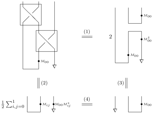
Figure 1: Relationship between the tangle relation (74) and the teleportation equation (36) or (91) in the topological diagrammatical representation. Let us explain the symbols (1), (2), (3) and (4), respectively. (1) The top two diagrams represent the tangle relation (82). (2) With the extended Temperley–Lieb configuration (55) of the Yang–Baxter gate $B$ and the constraint relation (78), the left-hand side of the tangle relation (74) can be simplified into the right-hand side of the teleportation equation (91), refer to both (84) and (90). (3) The right-hand side of the tangle relation (74) can be deformed into the left-hand side of the teleportation equation (91) with the topological straightening operation. (4) The bottom two diagrams represent the teleportation equation (91).

Therefore, in the extended Temperley–Lieb diagrammatical approach, the tangle relations (4) of the BMW algebra consisting of both the Temperley–Lieb projector and the Yang–Baxter gate admit an interesting interpretation of quantum teleportation. Note that such the relationship is independent of the specific representation of the Temperley–Lieb projector and the Yang–Baxter gate, such as (8) and (9) presented in the reference [22]. In view of this fact, furthermore, we will investigate the subject of how to derive a general representation of the BMW algebra in the extended Temperley–Lieb diagrammatical approach in the next section.

7 General construction of a representation of the tangle relations (4) of the BMW algebra

It is well-known that how to construct an interesting braid representation (2) (or an interesting solution of the Yang–Baxter equation [10]) is always a meaningful and challenge problem in the research frontier, refer to [9, 10, 11, 12, 13, 21, 34], and the same is true for the construction of an interesting representation of the BMW algebra [16], refer to [9, 17, 18, 19, 22, 23]. In the previous research [21], a method of constructing the Yang–Baxter gate in the extended Temperley–Lieb diagrammatical approach has been proposed, and hence in this section we want to exploit the extended Temperley–Lieb diagrammatical approach to construct interesting representations of the BMW algebra different from the representation using the Temperley–Lieb projector $E$ (8) and the Yang–Baxter gate $B$ (9). In view of the research result in the last section that the tangle relations (4) of the BMW algebra have a natural interpretation of quantum teleportation in the extended Temperley–Lieb diagrammatical approach, first of all, we focus on the general construction of the representation of the tangle relations (4) of the BMW algebra.

Looking at Theorem 1, we see that the tangle relations of the BMW algebra give rise to the constraint relations of single-qubit gates defining both the Temperley–Lieb projector and the Yang–Baxter gate. Hence we assume that the Temperley–Lieb projector $\tilde{E}$ and the Yang–Baxter gate $U$ have the form in terms of the Bell-like basis $|\Psi_{U_{ij}}\rangle$ given by

$$|\Psi_{U_{ij}}\rangle=(1\!\!1_{2}\otimes U_{ij})|\Psi\rangle$$ (95)

with single-qubit gates $U_{ij}$ satisfying the orthonormal condition

$$\frac{1}{2}\mathrm{tr}\left(U^{\dagger}_{i_{2}j_{2}}U_{i_{1}j_{1}}\right)=\delta_{i_{1}i_{2}}\delta_{j_{1}j_{2}},$$ (96)

and then require them to satisfy the tangle relations of the BMW algebra in order to derive the constraint equations of single-qubit gates $U_{ij}$.

Theorem 2.

The Temperley–Lieb projector $\tilde{E}$ assumes the form $\tilde{E}=|\Psi_{U_{mn}}\rangle\langle\Psi_{U_{mn}}|$ with specified $m,n$ and the Yang–Baxter gate $U$ assumes the form of the spectral decomposition given by

$$U=\sum_{i,j=0}^{1}\mu_{ij}|\Psi_{U_{ij}}\rangle\langle\Psi_{U_{ij}}|,$$ (97)

with eigenvalues $\mu_{ij}$. When single-qubit gates $U_{ij}$, $i,j=0,1$ and the specified single-qubit gate $U_{mn}$ satisfy the constraint relations:

$$\frac{1}{2}\sum_{k,l=0}^{1}\mu_{ij}\mu_{kl}U^{\dagger}_{mn}U_{kl}U_{ij}^{*}U_{mn}^{T}U^{\dagger}_{kl}U_{mn} = U^{*}_{ij}U^{T}_{mn};$$ (98)

$$\frac{1}{2}\sum_{k,l=0}^{1}\mu_{ij}\mu_{kl}U_{mn}^{*}U^{T}_{kl}U_{ij}^{\dagger}U_{mn}U^{*}_{kl}U^{T}_{mn} = U^{\dagger}_{ij}U_{mn};$$ (99)

$$\frac{1}{2}\sum_{k,l=0}^{1}\mu_{ij}\mu_{kl}U^{\dagger}_{mn}U_{kl}U_{mn}^{*}U_{ij}^{T}U^{\dagger}_{kl}U_{mn} = U^{*}_{mn}U^{T}_{ij};$$ (100)

$$\frac{1}{2}\sum_{k,l=0}^{1}\mu_{ij}\mu_{kl}U_{mn}^{*}U^{T}_{kl}U^{\dagger}_{mn}U_{ij}U^{*}_{kl}U^{T}_{mn} = U^{\dagger}_{mn}U_{ij},$$ (101)

the Temperley–Lieb projector $\tilde{E}$ and the Yang–Baxter gate $U$ satisfy the tangle relations (4) of the BMW algebra.

Proof.

The proof is a direct generalization of the proof for Theorem 1. For example, we derive the constraint relation (98) from the tangle relation using the Temperley–Lieb projector $\tilde{E}$ and the Yang–Baxter gate $U$ given by

$$(U\otimes 1\!\!1_{2})(1\!\!1_{2}\otimes U)(\tilde{E}\otimes 1\!\!1_{2})=2(1\!\!1_{2}\otimes\tilde{E})(\tilde{E}\otimes 1\!\!1_{2}).$$ (102)

Both sides of the equation (102) acting on $|\Psi_{M_{00}}\rangle\otimes|\alpha\rangle$ give rise to

$$\sum_{i,j=0}^{1}\sum_{k,l=0}^{1}\mu_{ij}\mu_{kl}\left((U_{ij},U^{\dagger}_{ij}),1\!\!1_{2}\right)\left(1\!\!1_{2},(U_{kl},U^{\dagger}_{kl})\right)\left(|\Psi_{U_{mn}}\rangle\otimes|\alpha\rangle\right)$$ (103)

$$= 2\left(1\!\!1_{2},(U_{mn},U^{\dagger}_{mn})\right)\left(|\Psi_{U_{mn}}\rangle\otimes|\alpha\rangle\right),$$

with the Bell-like projector $(U_{ij},U^{\dagger}_{ij})$ defined in (85), which can be simplified with the help of extended Temperley–Lieb configurations such as (38) and (90),

$$\frac{1}{4}\sum_{i,j=0}^{1}\sum_{k,l=0}^{1}|\Psi_{U_{ij}}\rangle\otimes\mu_{ij}\mu_{kl}U_{kl}U_{ij}^{*}U_{mn}^{T}U^{\dagger}_{kl}|\alpha\rangle=U^{T}_{mn}U^{\dagger}_{mn}|\alpha\rangle\otimes|\Psi_{U_{mn}}\rangle.$$ (104)

Furthermore, with the teleportation equation of describing the transport of the unknown qubit $|\beta\rangle=U^{T}_{mn}U^{\dagger}_{mn}|\alpha\rangle$,

$$|\beta\rangle\otimes|\Psi_{U_{mn}}\rangle=\frac{1}{2}\sum_{i,j=0}^{1}|\Psi_{U_{ij}}\rangle\otimes U_{mn}U^{*}_{ij}|\beta\rangle,$$ (105)

which can be derived with the extended Temperley–Lieb configuration (34), the equation (104) leads to the constraint relation of single-qubit gates $U_{ij}$,

$$\frac{1}{2}\sum_{k,l=0}^{1}\mu_{ij}\mu_{kl}U_{kl}U_{ij}^{*}U_{mn}^{T}U^{\dagger}_{kl}U_{mn}U^{*}_{mn}=U_{mn}U^{*}_{ij},$$ (106)

which is equivalent to (98). ∎

Corollary 2.

The eigenvalues $\mu_{ij}$ of the Yang–Baxter gate $U$ (97) satisfy the constraint relation

$$\frac{1}{2}\sum_{k,l=0}^{1}\mu_{mn}\mu_{kl}=1,$$ (107)

when the Temperley–Lieb projector $\tilde{E}$ and the Yang–Baxter gate $U$ satisfy the tangle relations (4) of the BMW algebra.

Proof.

The trace of the constraint relation (98) has the form

$$\frac{1}{2}\sum_{k,l=0}^{1}\mu_{ij}\mu_{kl}\mathrm{tr}\left(U^{\dagger}_{mn}U_{kl}U_{ij}^{*}U_{mn}^{T}U^{\dagger}_{kl}U_{mn}\right)=\mathrm{tr}\left(U^{*}_{ij}U^{T}_{mn}\right)$$ (108)

which leads to

$$\frac{1}{2}\sum_{k,l=0}^{1}\mu_{ij}\mu_{kl}\delta_{im}\delta_{jn}=\delta_{im}\delta_{jn},$$ (109)

where the orthonormal condition (96) for the Bell-like basis states $|\Psi_{U_{ij}}\rangle$ has been applied. Both sides of the constraint relation (109) have the summation over the indices $i$, $j$, which completes the proof for the corollary. ∎

As an example, we solve the constraint relations (98)-(101) to obtain interesting representations of the BMW algebra. The unitary bases $U_{ij}$ are set as $W_{ij}=X^{i}Z^{j}$ defining the Bell states $|\psi(ij)\rangle$ (11), and the unitary matrix $U_{mn}$ defining the Temperley–Lieb projector $\tilde{E}$ is also chosen as $U_{mn}=X^{m}Z^{n}$. The detailed calculation is shown in Appendix C, and the results are summarized as follows.

• The Temperley–Lieb projector $\tilde{E}$ has the form

  $$\tilde{E}=\frac{1}{2}\left(\begin{array}[]{cccc}1&0&0&\epsilon\\ 0&0&0&0\\ 0&0&0&0\\ \epsilon&0&0&1\\ \end{array}\right),$$ (110)

  where $\epsilon=1$ for $\tilde{E}=|\psi(00)\rangle\langle\psi(00)|$ and $\epsilon=-1$ for $\tilde{E}=|\psi(01)\rangle\langle\psi(01)|$, and the associated Yang–Baxter gate $U$ has the form

  $$U=\left(\begin{array}[]{cccc}\cos\phi&0&0&i\sin\phi\\ 0&-i\epsilon\sin\phi&\pm\cos\phi&0\\ 0&\pm\cos\phi&-i\epsilon\sin\phi&0\\ i\sin\phi&0&0&\cos\phi\\ \end{array}\right),$$ (111)

  or

  $$U=\left(\begin{array}[]{cccc}0&0&0&e^{i\phi}\\ 0&\epsilon e^{-i\phi}&0&0\\ 0&0&\epsilon e^{-i\phi}&0\\ e^{i\phi}&0&0&0\\ \end{array}\right),$$ (112)

  with $\phi\in[0,2\pi)$.

• The Temperley–Lieb projector $\tilde{E}$ has the form

  $$\tilde{E}=\frac{1}{2}\left(\begin{array}[]{cccc}0&0&0&0\\ 0&1&\epsilon&0\\ 0&\epsilon&1&0\\ 0&0&0&0\\ \end{array}\right),$$ (113)

  where $\epsilon=1$ for $\tilde{E}=|\psi(10)\rangle\langle\psi(10)|$ and $\epsilon=-1$ for $\tilde{E}=|\psi(11)\rangle\langle\psi(11)|$, and the corresponding Yang–Baxter gate $U$ has the form

  $$U=\left(\begin{array}[]{cccc}i\sin\phi&0&0&\cos\phi\\ 0&\pm\cos\phi&-i\epsilon\sin\phi&0\\ 0&-i\epsilon\sin\phi&\pm\cos\phi&0\\ \cos\phi&0&0&i\sin\phi\\ \end{array}\right),$$ (114)

  or

  $$U=\left(\begin{array}[]{cccc}e^{i\phi}&0&0&0\\ 0&0&\epsilon e^{-i\phi}&0\\ 0&\epsilon e^{-i\phi}&0&0\\ 0&0&0&e^{i\phi}\\ \end{array}\right),$$ (115)

  with $\phi\in[0,2\pi)$.

In the viewpoint of the extended Temperley–Lieb diagrammatical approach [21], Theorem 2 can be easily generalized. We consider the general case for the construction of the representation of the tangle relations (4) in which a two-qubit projective measurement operator $\tilde{E}$ and a two-qubit gate $G$ are involved, namely that the Temperley–Lieb projector $\tilde{E}$ and the Yang–Baxter gate $G$ are not supposed.

Theorem 3.

A two-qubit projector measurement operator $\tilde{E}=|\Psi_{U_{mn}}\rangle\langle\Psi_{U_{mn}}|$ and a two-qubit quantum gate $G$ given by

$$G=\sum_{i,j,k,l=0}^{1}\tilde{G}_{ij,kl}|\Psi_{U_{ij}}\rangle\langle\Psi_{U_{kl}}|$$ (116)

with 16 entries of complex numbers $\tilde{G}_{ij,kl}$ form the representation of the tangle relations (4) when the constraint relations

$$\frac{1}{2}\sum_{k_{1},l_{1}=0}^{1}\sum_{i_{2},j_{2},k_{2},l_{2}=0}^{1}\tilde{G}_{i_{1}j_{1},k_{1}l_{1}}\tilde{G}_{i_{2}j_{2},k_{2}l_{2}}U^{\dagger}_{mn}U_{i_{2}j_{2}}U^{*}_{k_{1}l_{1}}U^{T}_{mn}U_{k_{2}l_{2}}^{\dagger}U_{mn}= U^{*}_{i_{1}j_{1}}U^{T}_{mn};$$ (117)

$$\frac{1}{2}\sum_{k_{1},l_{1}=0}^{1}\sum_{i_{2},j_{2},k_{2},l_{2}=0}^{1}\tilde{G}_{i_{1}j_{1},k_{1}l_{1}}\tilde{G}_{i_{2}j_{2},k_{2}l_{2}}U^{*}_{mn}U^{T}_{i_{2}j_{2}}U^{\dagger}_{k_{1}l_{1}}U_{mn}U^{*}_{k_{2}l_{2}}U^{T}_{mn}= U^{\dagger}_{i_{1}j_{1}}U_{mn};$$ (118)

$$\frac{1}{2}\sum_{k_{1},l_{1}=0}^{1}\sum_{i_{2},j_{2},k_{2},l_{2}=0}^{1}\tilde{G}_{i_{1}j_{1},k_{1}l_{1}}\tilde{G}_{i_{2}j_{2},k_{2}l_{2}}U^{\dagger}_{mn}U_{i_{2}j_{2}}U^{*}_{mn}U^{T}_{k_{1}l_{1}}U_{k_{2}l_{2}}^{\dagger}U_{mn}= U^{*}_{mn}U^{T}_{i_{1}j_{1}};$$ (119)

$$\frac{1}{2}\sum_{k_{1},l_{1}=0}^{1}\sum_{i_{2},j_{2},k_{2},l_{2}=0}^{1}\tilde{G}_{i_{1}j_{1},k_{1}l_{1}}\tilde{G}_{i_{2}j_{2},k_{2}l_{2}}U^{*}_{mn}U^{T}_{i_{2}j_{2}}U^{\dagger}_{mn}U_{k_{1}l_{1}}U^{*}_{k_{2}l_{2}}U^{T}_{mn}= U^{\dagger}_{mn}U_{i_{1}j_{1}},$$ (120)

are satisfied.

The proof for Theorem 3 is a direct generalization of the proof for Theorem 2, and so it is omitted here. About how to solve these constraint relations to obtain an interesting representation of the tangle relations (4) is a challenge problem in future research, because the result may be not a representation of the BMW algebra but indeed has an interesting interpretation of quantum teleportation. In addition, the constraint relations (98)-(101) and the constraint relations (117)-(120) can be reformulated with the new conventions and notations, refer to Appendix D.

8 Concluding remarks

In this paper, we describe quantum teleportation protocol [3, 4, 5, 6] and teleportation-based quantum computation [24, 25] using the generators of the BMW algebra including both the Yang–Baxter gate and the Temperley–Lieb projector. We point out that the tangle relations defining the BMW algebra have a close connection with the teleportation process, and thus the extended Temperley–Lieb diagrammatical approach [20, 21] properly characterizes the topological feature of quantum teleportation. We propose a meaningful approach of constructing a general representation of the tangle relations of the BMW algebra and obtain interesting representations of the BMW algebra.

Notes Added. After this paper is done, we are occasionally informed that the Yang–Baxter gates (111) and (114) have been already presented in the preprint [34]. As a matter of fact, these gates are derived in two essentially different approaches. We derive such the Yang–Baxter gates in the extended Temperley–Lieb diagrammatical approach [20, 21], whereas the authors of [34] obtain them via the algebraic approach of the cyclic group. We study and look for interesting representations of the BMW algebra, which are not involved in [34].

Appendix A The Brauer algebra and quantum teleportation

It is well-known that the BMW algebra [16] is the algebraic deformation of the Brauer algebra [26]. Quantum teleportation using the Brauer algebra has been explored in [20], which originally motivated the authors to study quantum teleportation using the BMW algebra and write down the present paper. Here we make a simple sketch on the Brauer algebra and its relation to quantum teleportation.

The Brauer algebra $D_{n}(d)$ [26] with the loop parameter $d$ is generated by the Temperley–Lieb idempotents $e_{i}$ and the permutations $v_{i}$ with $i=1,\ldots,n-1$. The Temperley–Lieb idempotents $e_{i}$ satisfy the algebraic relations,

$$\begin{array}[]{ll}e_{i}^{2}=e_{i}&e_{i}e_{i\pm 1}e_{i}=d^{-2}e_{i},\\ e_{i}e_{j}=e_{j}e_{i}&|i-j|\geq 2,\end{array}$$ (121)

and the permutation generators $v_{i}$ satisfy

$$v_{i}^{2}=1\!\!1,\quad v_{i}v_{i\pm 1}v_{i}=v_{i\pm 1}v_{i}v_{i\pm 1}.$$ (122)

Both generators satisfy the first type of the mixed relations,

$$e_{i}v_{i}=v_{i}e_{i}=e_{i},$$ (123)

and the second type of the mixed relations,

$$v_{i\pm 1}v_{i}e_{i\pm 1}=e_{i}v_{i\pm 1}v_{i}=de_{i}e_{i\pm 1},$$ (124)

which are called the tangle relations of the Brauer algebra in this paper.

A tensor product representation of the Brauer algebra can be constructed in terms of the Bell state projector $|\Psi\rangle\langle\Psi|$ (11) and the permutation gate $P$ defined by $P|ij\rangle=|ji\rangle$ as follows

$$e_{i} = 1\!\!1^{\otimes(i-1)}\otimes|\Psi\rangle\langle\Psi|\otimes 1\!\!1^{\otimes(n-i-1)},$$ (125)

$$v_{i} = 1\!\!1^{\otimes(i-1)}\otimes P\otimes 1\!\!1^{\otimes(n-i-1)},$$ (126)

with the loop parameter $d=2$. Using the Bell state projector $|\Psi\rangle\langle\Psi|$, we perform the teleportation process in the way

$$(|\Psi\rangle\langle\Psi|\otimes 1\!\!1_{2})(|\alpha\rangle\otimes|\Psi\rangle)=\frac{1}{2}|\Psi\rangle\otimes|\alpha\rangle,$$ (127)

which is a special case of (30) for $i=j=0$. In terms of the permutation gate $P$, we define the teleportation operator as $(1\!\!1_{2}\otimes P)(P\otimes 1\!\!1_{2})$ to swap the quantum state in the way

$$(1\!\!1_{2}\otimes P)(P\otimes 1\!\!1_{2})(|\alpha\rangle\otimes|ij\rangle)=|ij\rangle\otimes|\alpha\rangle.$$ (128)

With the configuration (22) of the Bell state projector $|\Psi\rangle\langle\Psi|$ and the extended Temperley–Lieb configuration of the permutation gate $P$,

$$\begin{array}[]{c}\begin{picture}(130.0,32.0)\par\put(20.0,16.0){$P=\sum_{i,j=0}^{1}(-1)^{i\cdot j}$} \par\put(92.0,18.0){\line(0,1){12.0}} \put(82.0,18.0){\line(0,1){12.0}} \put(82.0,18.0){\line(1,0){10.0}} \put(92.0,24.0){\circle*{2.0}} \put(94.0,23.0){\tiny{$W_{ij}$}} \put(82.0,0.0){\line(0,1){12.0}} \put(92.0,0.0){\line(0,1){12.0}} \put(82.0,12.0){\line(1,0){10.0}} \put(92.0,6.0){\circle*{2.0}} \put(94.0,5.0){\tiny{$W^{\dagger}_{ij}$}} \put(110.0,12.0){,} \end{picture}\end{array}$$ (129)

we reformulate the tangle relations (124) of the Brauer algebra as

$$(P\otimes 1\!\!1_{2})(1\!\!1_{2}\otimes P)\left(|\Psi\rangle\otimes|\alpha\rangle\right)=2(1\!\!1_{2}\otimes|\Psi\rangle\langle\Psi|)\left(|\Psi\rangle\otimes|\alpha\rangle\right)$$ (130)

which can be reduced into the teleportation equation (31), refer to the proof for Corollary 1.

When the permutation gate $P$ is replaced with the Yang–Baxter gate $B$ (9), the above representation of the Brauer algebra is substituted by the representation of the BMW algebra, so the study of quantum teleportation using the Brauer algebra in [20] naturally points towards the study of quantum teleportation using the BMW algebra in this paper.

Appendix B More on the extended Temperley–Lieb configurations of the Yang–Baxter gate $B$ (9)

It is obvious that the extended Temperley–Lieb configurations [20, 21] play the essential roles throughout this paper. In accordance with the reference [21], a Yang–Baxter gate allows various but equivalent extended Temperley–Lieb configurations. For example, three distinct configurations of the Yang–Baxter gate $B$ (9) are presented in Subsection 4.2. Here another two extended Temperley–Lieb configurations of the Yang–Baxter gate $B$ are introduced and they may be useful elsewhere.

The Yang–Baxter gate $B$ (9) can be related to the Temperley–Lieb projector $E$ (8) in the way

$$B=\tilde{U}+2ie^{i\frac{3}{4}\pi}E,$$ (131)

where $\tilde{U}$ is a unitary matrix with the decomposition

$$\tilde{U}=e^{i\frac{3}{4}\pi}1\!\!1_{4}+\sqrt{2}\left(|\psi(10)\rangle\langle\psi(10)|+|\Psi_{R_{2\phi}}\rangle\langle\Psi_{R_{2\phi}}|\right),$$ (132)

with $|\psi(10)\rangle=(1\!\!1_{2}\otimes X)|\Psi\rangle$ and $|\Psi_{R_{2\phi}}\rangle=(1\!\!1_{2}\otimes R_{2\phi})|\Psi\rangle$, $R_{2\phi}$ denoting the phase shift gate (16), and the associated extended Temperley–Lieb configuration is illustrated in

$$\begin{array}[]{c}\begin{picture}(130.0,40.0)\par\put(-25.0,-2.0){\footnotesize{$B$}} \par\put(-31.0,29.0){\line(0,1){6.0}} \put(-31.0,11.0){\line(0,-1){6.0}} \put(-13.0,29.0){\line(0,1){6.0}} \put(-13.0,11.0){\line(0,-1){6.0}} \par\put(-34.0,8.0){\line(0,1){24.0}} \put(-10.0,8.0){\line(0,1){24.0}} \put(-34.0,8.0){\line(1,0){24.0}} \put(-34.0,32.0){\line(1,0){24.0}} \par\par\par\put(-31.0,29.0){\line(1,-1){18.0}} \put(-31.0,11.0){\line(1,1){7.3}} \put(-13.0,29.0){\line(-1,-1){7.3}} \par\par\put(-3.0,19.0){$=e^{i\frac{3}{4}\pi}$} \par\put(32.0,5.0){\line(0,1){30.0}} \put(22.0,5.0){\line(0,1){30.0}} \par\par\put(40.0,19.0){$+\sqrt{2}$} \par\put(72.0,23.0){\line(0,1){12.0}} \put(62.0,23.0){\line(0,1){12.0}} \put(62.0,23.0){\line(1,0){10.0}} \put(72.0,29.0){\circle*{2.0}} \put(74.0,28.0){\tiny{$X$}} \par\put(62.0,5.0){\line(0,1){12.0}} \put(72.0,5.0){\line(0,1){12.0}} \put(62.0,17.0){\line(1,0){10.0}} \put(72.0,11.0){\circle*{2.0}} \put(74.0,10.0){\tiny{$X$}} \par\put(80.0,19.0){$+\sqrt{2}$} \par\put(112.0,23.0){\line(0,1){12.0}} \put(102.0,23.0){\line(0,1){12.0}} \put(102.0,23.0){\line(1,0){10.0}} \put(112.0,29.0){\circle*{2.0}} \put(114.0,28.0){\tiny{$R_{2\phi}$}} \par\put(102.0,5.0){\line(0,1){12.0}} \put(112.0,5.0){\line(0,1){12.0}} \put(102.0,17.0){\line(1,0){10.0}} \put(112.0,11.0){\circle*{2.0}} \put(114.0,10.0){\tiny{$R^{\dagger}_{2\phi}$}} \par\put(118.0,19.0){$+2ie^{i\frac{3}{4}\pi}$} \par\put(156.0,23.0){\line(0,1){12.0}} \put(146.0,23.0){\line(0,1){12.0}} \put(146.0,23.0){\line(1,0){10.0}} \put(156.0,29.0){\circle*{2.0}} \put(158.0,28.0){\tiny{$M_{00}$}} \par\put(146.0,5.0){\line(0,1){12.0}} \put(156.0,5.0){\line(0,1){12.0}} \put(146.0,17.0){\line(1,0){10.0}} \put(156.0,11.0){\circle*{2.0}} \put(158.0,10.0){\tiny{$M_{00}^{\dagger}$}} \par\end{picture}\end{array}$$ (133)

where the two vertical lines represent for the identity matrix $1\!\!1_{4}$.

Note that the single-qubit gate $M_{00}$ is defined as $M_{00}=R_{\phi}HSHR_{\phi}$ (18). And bring such decomposition of the $M_{00}$ gate into the relation (131). After some algebra, the Yang–Baxter gate $B$ takes another form

$$B=e^{i\frac{3}{4}\pi}\left(1\!\!1_{4}-|\psi(10)\rangle\langle\psi(10)|-|\Psi_{R_{2\phi}}\rangle\langle\Psi_{R_{2\phi}}|-e^{-i\phi}|\Psi_{R_{2\phi}}\rangle\langle\psi(10)|+e^{i\phi}|\psi(10)\rangle\langle\Psi_{R_{2\phi}}|\right),$$ (134)

and its extended Temperley–Lieb configuration is shown below

$$\begin{array}[]{c}\begin{picture}(135.0,40.0)\par\put(-25.0,-2.0){\footnotesize{$B$}} \par\put(-31.0,29.0){\line(0,1){6.0}} \put(-31.0,11.0){\line(0,-1){6.0}} \put(-13.0,29.0){\line(0,1){6.0}} \put(-13.0,11.0){\line(0,-1){6.0}} \par\put(-34.0,8.0){\line(0,1){24.0}} \put(-10.0,8.0){\line(0,1){24.0}} \put(-34.0,8.0){\line(1,0){24.0}} \put(-34.0,32.0){\line(1,0){24.0}} \par\put(-31.0,29.0){\line(1,-1){18.0}} \put(-31.0,11.0){\line(1,1){7.3}} \put(-13.0,29.0){\line(-1,-1){7.3}} \par\put(-6.0,19.0){$=e^{i\frac{3}{4}\pi}($} \par\put(32.0,5.0){\line(0,1){30.0}} \put(22.0,5.0){\line(0,1){30.0}} \par\par\put(40.0,19.0){$-$} \par\put(62.0,23.0){\line(0,1){12.0}} \put(52.0,23.0){\line(0,1){12.0}} \put(52.0,23.0){\line(1,0){10.0}} \put(62.0,29.0){\circle*{2.0}} \put(64.0,28.0){\tiny{$X$}} \par\put(52.0,5.0){\line(0,1){12.0}} \put(62.0,5.0){\line(0,1){12.0}} \put(52.0,17.0){\line(1,0){10.0}} \put(62.0,11.0){\circle*{2.0}} \put(64.0,11.0){\tiny{$X$}} \par\put(70.0,19.0){$-$} \par\put(92.0,23.0){\line(0,1){12.0}} \put(82.0,23.0){\line(0,1){12.0}} \put(82.0,23.0){\line(1,0){10.0}} \put(92.0,29.0){\circle*{2.0}} \put(94.0,28.0){\tiny{$R_{2\phi}$}} \par\put(82.0,5.0){\line(0,1){12.0}} \put(92.0,5.0){\line(0,1){12.0}} \put(82.0,17.0){\line(1,0){10.0}} \put(92.0,11.0){\circle*{2.0}} \put(94.0,10.0){\tiny{$R^{\dagger}_{2\phi}$}} \par\put(95.0,19.0){$-e^{-i\phi}$} \par\put(127.0,23.0){\line(0,1){12.0}} \put(117.0,23.0){\line(0,1){12.0}} \put(117.0,23.0){\line(1,0){10.0}} \put(127.0,29.0){\circle*{2.0}} \put(129.0,28.0){\tiny{$R_{2\phi}$}} \par\put(117.0,5.0){\line(0,1){12.0}} \put(127.0,5.0){\line(0,1){12.0}} \put(117.0,17.0){\line(1,0){10.0}} \put(127.0,11.0){\circle*{2.0}} \put(129.0,10.0){\tiny{$X$}} \par\put(133.0,19.0){$+e^{i\phi}$} \par\put(162.0,23.0){\line(0,1){12.0}} \put(152.0,23.0){\line(0,1){12.0}} \put(152.0,23.0){\line(1,0){10.0}} \put(162.0,29.0){\circle*{2.0}} \put(164.0,28.0){\tiny{$X$}} \par\put(152.0,5.0){\line(0,1){12.0}} \put(162.0,5.0){\line(0,1){12.0}} \put(152.0,17.0){\line(1,0){10.0}} \put(162.0,11.0){\circle*{2.0}} \put(164.0,10.0){\tiny{$R^{\dagger}_{2\phi}$}} \par\put(169.0,19.0){$)$} \par\end{picture}\end{array}$$ (135)

which together with (133) point out the fact that no transparent topological deformations exist between such two configurations, although they are algebraically equivalent.

Appendix C How to solve the constraint relation (98)

For example, we make a sketch on how to derive the representation of the BMW algebra, such as (110) and (111) or (112) from the constraint relation (98). Set the unitary bases $U_{ij}$ as $U_{ij}=X^{i}Z^{j}$ and the unitary base matrix $U_{mn}$ as $U_{mn}=1\!\!1_{2}$. Then the constraint relation (98) has the form

$$\frac{1}{2}\sum_{k,l=0}^{1}\mu_{ij}\mu_{kl}X^{k}Z^{l}X^{i}Z^{j}Z^{l}X^{k}=X^{i}Z^{j},$$ (136)

which can be reformulated as

$$\frac{1}{2}\sum_{k,l=0}^{1}\mu_{ij}\mu_{kl}(-1)^{i\cdot l}(-1)^{k\cdot j}X^{i}Z^{j}=X^{i}Z^{j}.$$ (137)

Since the unitary bases $U_{ij}$ satisfy the orthonormal relation (96), we have the constraint equation of the eigenvalues $\mu_{ij}$ of the Yang–Baxter gate $U$ (97),

$$\sum_{k,l=0}^{1}\mu_{ij}\mu_{kl}(-1)^{i\cdot l}(-1)^{k\cdot j}=2,$$ (138)

which represent a set of equations given by

$$\mu_{00}\left(\mu_{00}+\mu_{01}+\mu_{10}+\mu_{11}\right) = 2;$$ (139)

$$\mu_{01}\left(\mu_{00}+\mu_{01}-\mu_{10}-\mu_{11}\right) = 2;$$ (140)

$$\mu_{10}\left(\mu_{00}-\mu_{01}+\mu_{10}-\mu_{11}\right) = 2;$$ (141)

$$\mu_{11}\left(\mu_{00}-\mu_{01}-\mu_{10}+\mu_{11}\right) = 2.$$ (142)

Solving the above equations, we have three classes of solutions for the eigenvalues $\mu_{ij}$ as below.

• Class 1: $\mu_{00}=e^{i\phi}$, $\mu_{01}=e^{-i\phi}$, $\mu_{10}=e^{-i\phi}$, $\mu_{11}=-e^{i\phi}$, which determine the Yang–Baxter gate $U$ (97) as

  $$U=\sum_{i,j=0}^{1}\mu_{ij}|\psi(ij)\rangle\langle\psi(ij)|=\left(\begin{array}[]{cccc}\cos\phi&0&0&i\sin\phi\\ 0&-i\sin\phi&\cos\phi&0\\ 0&\cos\phi&-i\sin\phi&0\\ i\sin\phi&0&0&\cos\phi\\ \end{array}\right).$$ (143)

• Class 2: $\mu_{00}=e^{i\phi}$, $\mu_{01}=e^{-i\phi}$, $\mu_{10}=-e^{i\phi}$, $\mu_{11}=e^{-i\phi}$, which determine the Yang–Baxter gate $U$ (97) as

  $$U=\sum_{i,j=0}^{1}\mu_{ij}|\psi(ij)\rangle\langle\psi(ij)|=\left(\begin{array}[]{cccc}\cos\phi&0&0&i\sin\phi\\ 0&-i\sin\phi&-\cos\phi&0\\ 0&-\cos\phi&-i\sin\phi&0\\ i\sin\phi&0&0&\cos\phi\\ \end{array}\right).$$ (144)

• Class 3: $\mu_{00}=e^{i\phi}$, $\mu_{01}=-e^{i\phi}$, $\mu_{10}=e^{-i\phi}$, $\mu_{11}=e^{-i\phi}$, which determine the Yang–Baxter gate $U$ (97) as

  $$U=\sum_{i,j=0}^{1}\mu_{ij}|\psi(ij)\rangle\langle\psi(ij)|=\left(\begin{array}[]{cccc}0&0&0&e^{i\phi}\\ 0&e^{-i\phi}&0&0\\ 0&0&e^{-i\phi}&0\\ e^{i\phi}&0&0&0\\ \end{array}\right).$$ (145)

Similarly, when the unitary bases $U_{mn}$ are the Pauli gates $X$, $Z$ and $XZ$, respectively, the other solutions of the Yang–Baxter gate $U$ (97) can be obtained. The collection of all the solutions has been presented in (110) and (111) or (112), or (113) and (114) or (115).

Appendix D Reformulation of the constraint relations (98)-(101) and (117)-(120)

Both the constraint relations (98)-(101) and the constraint relations (117)-(120) looking complicated, we introduce the new conventions to simplify their formulations. We define the skew-transpose on the product of two matrices as

$$(B\,C)^{ST}\equiv B^{T}\,C^{T},$$ (146)

where the skew-transposition $ST$ does not interchange $B^{T}$ and $C^{T}$ as the ordinary transpose does. With the new notations given by

$$\eta_{ijkl}\equiv\frac{1}{2}\mu_{ij}\mu_{kl};\quad O_{\alpha\beta}\equiv U^{\dagger}_{mn}U_{\alpha\beta},$$ (147)

with specified indices $m$ and $n$, the constraint relations (98)-(101) have the simplified forms

$$\sum_{k,l=0}^{1}\eta_{ijkl}O_{kl}{O^{ST}_{ij}}^{\dagger}O^{\dagger}_{kl} = {O^{ST}_{ij}}^{\dagger};$$ (148)

$$\sum_{k,l=0}^{1}\eta_{ijkl}O^{ST}_{kl}O^{\dagger}_{ij}{O_{kl}^{ST}}^{\dagger} = O^{\dagger}_{ij};$$ (149)

$$\sum_{k,l=0}^{1}\eta_{ijkl}O_{kl}O^{ST}_{ij}O_{kl}^{\dagger} = O^{ST}_{ij};$$ (150)

$$\sum_{k,l=0}^{1}\eta_{ijkl}O^{ST}_{kl}O_{ij}{O_{kl}^{ST}}^{\dagger} = O_{ij},$$ (151)

where the skew-transpose $ST$ is commutative with the Hermitian conjugation ${\dagger}$. As a remark, the notation $O_{\alpha\beta}$ is introduced to remove the indices $m$ and $n$ so that the algebraic structure of the constraint relations (98)-(101) is presented in a more transparent way. Furthermore, with the new notation

$$\eta_{i_{1}j_{1}i_{2}j_{2}k_{1}l_{1}k_{2}l_{2}}\equiv\frac{1}{2}G_{i_{1}j_{1},k_{1}l_{1}}\tilde{G}_{i_{2}j_{2},k_{2}l_{2}},$$ (152)

the constraint relations (117)-(120) have more simplified forms

$$\sum_{k,l=0}^{1}\eta_{i_{1}j_{1}i_{2}j_{2}k_{1}l_{1}k_{2}l_{2}}O_{i_{2}j_{2}}{O^{ST}_{k_{1}l_{1}}}^{\dagger}O^{\dagger}_{k_{2}l_{2}} = {O^{ST}_{i_{1}j_{1}}}^{\dagger};$$ (153)

$$\sum_{k,l=0}^{1}\eta_{i_{1}j_{1}i_{2}j_{2}k_{1}l_{1}k_{2}l_{2}}O^{ST}_{i_{2}j_{2}}O^{\dagger}_{k_{1}l_{1}}{O_{k_{2}l_{2}}^{ST}}^{\dagger} = O^{\dagger}_{i_{1}j_{1}};$$ (154)

$$\sum_{k,l=0}^{1}\eta_{i_{1}j_{1}i_{2}j_{2}k_{1}l_{1}k_{2}l_{2}}O_{i_{2}j_{2}}O^{ST}_{k_{1}l_{1}}O_{k_{2}l_{2}}^{\dagger} = O^{ST}_{i_{1}j_{1}};$$ (155)

$$\sum_{k,l=0}^{1}\eta_{i_{1}j_{1}i_{2}j_{2}k_{1}l_{1}k_{2}l_{2}}O^{ST}_{i_{2}j_{2}}O_{k_{1}l_{1}}{O_{k_{2}l_{2}}^{ST}}^{\dagger} = O_{i_{1}j_{1}}.$$ (156)

As a concluding remark, we hope that such the above reformulations of the constraint relations (98)-(101) and (117)-(120) are meaningful and useful elsewhere.

References

• [1] M.A. Nielsen and I.L. Chuang, Quantum Computation and Quantum Information (Cambridge University Press, Cambridge, UK, 2000 and 2011).
• [2] J. Preskill, Lecture Notes on Quantum Computation, http://www.theory.caltech.edu/preskill.
• [3] C.H. Bennett, G. Brassard, C. Crepeau, R. Jozsa, A. Peres and W.K. Wootters, Teleporting an Unknown Quantum State via Dual Classical and Einstein-Podolsky-Rosen Channels, Phys. Rev. Lett. 70, 1895 (1993).
• [4] L. Vaidman, Teleportation of Quantum States, Phys. Rev. A 49, 1473-1475 (1994).
• [5] S.L. Braunstein, G.M. D’Ariano, G.J. Milburn and M.F. Sacchi, Universal Teleportation with a Twist, Phys. Rev. Lett. 84, 3486-3489 (2000).
• [6] R.F. Werner, All Teleportation and Dense Coding Schemes, J. Phys. A: Math. Theor. 35, 7081-7094 (2001).
• [7] P.K. Aravind, Borromean Entanglement of the GHZ State, in Potentiality, Entanglement and Passion-at-a-Distance, Springer Netherlands, 53-59 (1997).
• [8] L.H. Kauffman and S.J. Lomonaco Jr., Quantum Entanglement and Topological Entanglement, New J. Phys. 4, 73 (2002).
• [9] L.H. Kauffman, Knots and Physics (World Scientific Publishers, 2002).
• [10] C.N. Yang, Some Exact Results for the Many Body Problems in One Dimension with Repulsive Delta Function Interaction, Phys. Rev. Lett. 19, 1312-1314 (1967). R.J. Baxter, Partition Function of the Eight-Vertex Lattice Model, Ann. Phys. 70, 193-228 (1972). J.H.H. Perk and H. Au-Yang, Yang–Baxter Equations, Encyclopedia of Mathematical Physics, Vol. 5, 465-473 (Elsevier Science, Oxford, 2006).
• [11] H. Dye, Unitary Solutions to the Yang–Baxter Equation in Dimension Four, Quantum Inf. Process. 2, 117-150 (2003).
• [12] L.H. Kauffman and S.J. Lomonaco Jr., Braiding Operators are Universal Quantum Gates, New J. Phys. 6, 134 (2004).
• [13] Y. Zhang, L.H. Kauffman and M.L. Ge, Universal Quantum Gate, Yang–Baxterization and Hamiltonian, Int. J. Quant. Inform. 4, 669-678 (2005).
• [14] G. Alagic, M. Jarret and S.P. Jordan, Yang–Baxter Operators Need Quantum Entanglement to Distinguish Knots, J. Phys. A: Math. Theor. 49, 075203 (2016).
• [15] H.N.V. Temperley and E.H. Lieb, Relations between the ‘Percolation’ and ‘Colouring’ Problem and Other Graph-Theoretical Problems Associated with Regular Planar Lattices: Some Exact Results for the ‘Percolation’ Problem, Proc. Roy. Soc. A 322, 251 (1971).
• [16] J.S. Birman and H.B. Wenzl, Link Polynomials and a New Algebra, Transactions of the American Mathematical Society 313, 249-273 (1989). J. Murakami, The Kauffman Polynomial of Links and Representation Theory, Osaka J. Math 24, 745-758 (1987).
• [17] V. Jones, On a Certain Value of the Kauffman Polynomial, Commun. Math. Phys. 125, 459-467 (1989).
• [18] Y. Cheng, M.L. Ge and K. Xue, Yang–Baxterization of Braid Group Representations, Commun. Math. Phys. 136, 195-208 (1991).
• [19] G. Wang, K. Xue, C. Sun, C. Zhou, T. Hu and Q. Wang, Temperley–Lieb Algebra, Yang–Baxterization and Universal Gate, Quantum Inf. Process. 9, 699-710 (2010).
• [20] Y. Zhang, Teleportation, Braid Group and Temperley–Lieb Algebra, J. Phys. A: Math. Theor. 39, 11599-11622 (2006). Y. Zhang and L.H. Kauffman, Topological-Like Features in Diagrammatical Quantum Circuits, Quantum Inf. Process. 6, 477-507 (2007). Y. Zhang, Braid Group, Temperley–Lieb Algebra, and Quantum Information and Computation, AMS Contemporary Mathematics 482, 52 (2009).
• [21] Y. Zhang, K. Zhang and J.-L. Pang, Teleportation-Based Quantum Computation, Extended Temperley–Lieb Diagrammatical Approach and Yang–Baxter Equation, Quantum Inf. Process. 15, 405-464 (2016).
• [22] G. Wang, K. Xue, C. Sun, B. Liu, Y. Liu, and Y. Zhang, Topological Basis Associated with B-M-W algebra: Two Spin-1/2 Realization, Phys. Lett. A 379, 1-4 (2015).
• [23] C. Zhou, K. Xue, G. Wang, C. Sun and G. Du, Birman-Wenzl-Murakami Algebra and Topological Basis, Communications in Theoretical Physics 57, 179 (2012). C. Zhou, K. Xue, L. Gou, C. Sun, G. Wang and T. Hu, Birman-Wenzl-Murakami Algebra, Topological Parameter and Berry Phase, Quantum Inf. Process. 11, 1765-1773 (2012). Q. Zhao, R.Y. Zhang, K. Xue and M.L. Ge, Topological Basis Associated with BWMA, Extremes of $L_{1}$-norm in Quantum Information and Applications in Physics, arXiv:1211.6178 (2012).
• [24] D. Gottesman and I.L. Chuang, Demonstrating the Viability of Universal Quantum Computation Using Teleportation and Single-Qubit Operations, Nature 402, 390 (1999).
• [25] M.A. Nielsen, Universal Quantum Computation Using Only Projective Measurement, Quantum Memory, and Preparation of the 00 State, Phys. Lett. A 308, 96 (2003).
• [26] R. Brauer, On Algebras Which are Connected With the Semisimple Continuous Groups, Ann. of Math. 38, 857-872 (1937).
• [27] Y. Zhang and K. Zhang, GHZ transform (I): Bell transform and quantum teleportation, arXiv:1401.7009 (2014).
• [28] K.G.H. Vollbrecht and R.F. Werner, Why Two Qubits are Special, Journal of Mathematical Physics 41, 6772-6782 (2000).
• [29] B. Kraus and J.I. Cirac, Optimal Creation of Entanglement Using a Two-Qubit Gate, Phys. Rev. A 63, 062309 (2001).
• [30] P. Zanardi, C. Zalka and L. Faoro, Entangling Power of Quantum Evolutions, Phys. Rev. A 62, 030301 (2000).
• [31] V.V. Shende, S.S. Bullock and I.L. Markov, Recognizing Small-Circuit Structure in Two-Qubit Operators, Phys. Rev. A 70, 012310 (2004).
• [32] D. Gottesman, Stabilizer Codes and Quantum Error Correction Codes, Ph.D. Thesis, CalTech, Pasadena, CA, 1997.
• [33] P.O. Boykin, T. Mor, M. Pulver, V. Roychowdhury and F. Vatan, A New Universal and Fault-Tolerant Quantum Basis, Inf. Process. Lett, 75, 101-107 (2000).
• [34] A. Pourkia, J. Batle and C.H. Raymond Ooi, Cyclic Groups and Quantum Logic Gates, arXiv:1509.08252 (2015).