LPTENS–16/04, CPHT–RR033.062016,  July 2016

Super no-scale models in string theory

Costas Kounnas¹ and Hervé Partouche²

¹ Laboratoire de Physique Théorique, Ecole Normale Supérieure^†,
24 rue Lhomond, F–75231 Paris cedex 05, France
Costas.Kounnas@lpt.ens.fr

² Centre de Physique Théorique, Ecole Polytechnique, CNRS, Université Paris-Saclay
F–91128 Palaiseau cedex, France
herve.partouche@polytechnique.edu

 

Abstract

We consider “super no-scale models” in the framework of the heterotic string, where the ${\cal N}=4,2,1\to 0$ spontaneous breaking of supersymmetry is induced by geometrical fluxes realizing a stringy Scherk-Schwarz perturbative mechanism. Classically, these backgrounds are characterized by a boson/fermion degeneracy at the massless level, even if supersymmetry is broken. At the 1-loop level, the vacuum energy is exponentially suppressed, provided the supersymmetry breaking scale is small, $m_{3/2}\ll M_{\rm string}$. We show that the “super no-scale string models” under consideration are free of Hagedorn-like tachyonic singularities, even when the supersymmetry breaking scale is large, $m_{3/2}\simeq M_{\rm string}$. The vacuum energy decreases monotonically and converges exponentially to zero, when $m_{3/2}$ varies from $M_{\rm string}$ to $0$. We also show that all Wilson lines associated to asymptotically free gauge symmetries are dynamically stabilized by the 1-loop effective potential, while those corresponding to non-asymtotically free gauge groups lead to instabilities and condense. The Wilson lines of the conformal gauge symmetries remain massless. When stable, the stringy super no-scale models admit low energy effective actions, where decoupling gravity yields theories in flat spacetime, with softly broken supersymmetry.

 ^† Unité mixte du CNRS et de l’Ecole Normale Supérieure associée à l’Université Pierre et Marie Curie (Paris 6), UMR 8549.

1 Introduction and summary

String theory unifies gravitational and gauge interactions at the quantum level. To describe particle physics, one can naturally consider classical models defined in four-dimensional Minkowski spacetime, where string perturbation theory can be implemented to derive the quantum dynamics. However, from a gravitational point of view, the question of the cosmological constant which can be regenerated at 1-loop, must be addressed. In non-supersymmetric models, such as those derived by compactifying the $SO(16)\times SO(16)$ ten-dimensional heterotic string, this vacuum energy density is extremely large [1]. It is generically of order $M_{\rm s}^{4}$, where $M_{\rm s}$ is the string scale, and has no chance to be naturally cancelled by any mechanism involving physics at lower energy.

Alternatively, one can consider no-scale models [2], which by definition describe at tree level theories in Minkowski space, where supersymmetry is spontaneously broken at an arbitrary scale $m_{3/2}$. More precisely, $m_{3/2}$ is a flat direction of a classical positive semi-definite potential, ${\cal V}_{\rm tree}\geq 0$. This very fact opens the possibility to generate by quantum effects a vacuum energy of arbitrary magnitude. In ${\cal N}=1$ supergravity language, the no-scale models involve a superpotential $w_{0}$ and moduli fields $z_{i}$, in terms of which the scale of the spontaneous supersymmetry breaking can be expressed as[3],

$$m^{2}_{3/2}=e^{K}|w_{0}|^{2}={e^{\tilde{K}}|w_{0}|^{2}\over{\rm Im}\,z_{1}\,{\rm Im}\,z_{2}\,{\rm Im}\,z_{3}}\,,$$ (1.1)

where $K$ is the Kälher potential and $\tilde{K}$ is the part of $K$ that is independent of the three moduli $z_{i}$ associated to the breaking of supersymmetry. When $w_{0}$ is independent of the $z_{i}$’s, $m_{3/2}$ is undetermined by the minimization condition $\langle{\cal V}_{\rm tree}\rangle=0$. In string theory or its associated effective supergravity description at low energy, depending on the choice of supersymmetry breaking mechanism, the $z_{i}$’s can either be the dilaton-axion field $S$, or Kähler or complex structure moduli $T_{I},U_{I}$ associated to the six-dimensional internal space. For instance :

- Some initially supersymmetric models can develop non-perturbative effects, such as gaugino condensation[4]. In this case, some of the fields, including $S$, are stabilized. The magnitude of supersymmetry breaking is determined by $|w_{0}|^{2}={\Lambda_{\rm np}^{6}/M_{\rm P}^{4}}$ and the imaginary parts of $z_{i}$, $i\in\{1,2,3\}$, which can be Kähler or complex structure moduli $T_{I},U_{I}$. In the expression of the superpotential, $M_{\rm P}\simeq 2.4\cdot 10^{18}$ GeV is the Planck scale and $\Lambda_{\rm np}=M_{\rm s}\exp{(-8\pi^{2}/|b|g_{\rm s}^{2})}$ is the scale of confinement associated to an asymptotically free gauge group, of $\beta$-function coefficient $b$. $g_{\rm s}$ is the string coupling, which relates the string and Planck scales as $M_{\rm s}=g_{\rm s}M_{\rm P}$. The gaugino condensation breaking mechanism leads naturally to a small gravitino mass, even though the moduli fields ${\rm Im}\,z_{i}$’s are of order 1. However, this non-perturbative scenario can only be studied qualitatively at the effective supergravity level, since no fully quantitative derivation from string computations is available yet.

- Alternatively, perturbative or non-perturbative fluxes [5] along the internal space can induce non-trivial superpotentials that break supersymmetry. In some cases, S-,T- or U-dualities [6] can be used to derive semi-quantitative results. In general, there is not yet available full derivation from string computations and so, one must restrict to semi-quantitative descriptions at the effective supergravity level. Some exception however exists, on which we now turn on.

In the present work, we focus on geometrical fluxes that realize generalized “coordinate-dependent compactifications” [7, 8]. The latter are similar to that proposed by Scherk and Schwarz in supergravity [9], but upgraded to string theory and furthermore to its gauge sector. In some cases, the mechanism can be implemented at the level of the worldsheet 2-dimensional conformal field theory, thus allowing explicit quantitative string computations, order by order in perturbation. The scale $m_{3/2}$ of spontaneous supersymmetry breaking is given by the inverse volume of the internal directions involved in the generalized stringy Scherk-Schwarz mechanism. For the quantum vacuum energy density to not be of order $M_{\rm s}^{4}$, this volume should be large, and the associated towers of Kaluza-Klein (KK) states should be light, with many consequences :

$\bullet$ When their contributions do not cancel each another (a situation that will be central to the present work), the KK states, whose masses are of order $m_{3/2}$, dominate the quantum amplitudes, while the heavier states, whose masses are of order $cM_{\rm s}$, yield exponentially suppressed contributions, ${\cal O}(e^{-cM_{\rm s}/m_{3/2}})$. In practice, $cM_{\rm s}$ can be the string scale, the GUT scale or a large Higgs scale.

$\bullet$ These dominant contributions are the full expressions obtained in loop computations done in a pure KK field theory that realizes a spontaneous breaking of supersymmetry à la Scherk-Schwarz. No UV divergence occurs, a fact that is similar to that observed in field theory at finite temperature when the KK modes are Matsubara excitations along the Euclidean time circle and the spectrum at zero temperature is supersymmetric.

$\bullet$ At 1-loop, if the model does not contain any scale below $m_{3/2}$, the effective potential takes the form [10, 11, 12, 13],

$${\cal V}_{\mbox{\scriptsize 1-loop}}=\xi(n_{\rm F}-n_{\rm B})\,m_{3/2}^{4}+{\cal O}\!\left(M_{\rm s}^{4}\,e^{-cM_{\rm s}/m_{3/2}}\right),$$ (1.2)

where $n_{\rm F}$ and $n_{\rm B}$ count the numbers of massless fermionic and bosonic degrees of freedom, while $\xi>0$ depends on moduli fields other than $m_{3/2}$. The above result makes sense in the theories that are free of “decompactification problems” [14], which would invalidate the string perturbative approach, due to large threshold corrections to gauge couplings [15, 16]. For instance, models realizing either the ${\cal N}=4\to 0$ or ${\cal N}=4\to 2\to 0$ or ${\cal N}=2\to 1\to 0$ patterns of spontaneous supersymmetry breaking are consistent at the perturbative level [13].

Notice in Eq. (1.2) the absence of term proportional to $\textrm{Str}\,M^{2}\,\Lambda^{2}_{\rm co}\propto m_{3/2}^{2}\Lambda^{2}_{\rm co}$, where $M$ is the mass operator. Such a term appears in ${\cal N}=1$ and ${\cal N}=2$ supergravities spontaneously broken to ${\cal N}=0$, when the quantum corrections are regularized in the UV by a cut-off scale $\Lambda^{2}_{\rm co}={\cal O}(M^{2}_{\rm s})$. Even if the extremely large term $m_{3/2}^{2}\Lambda^{2}_{\rm co}$ is not present in string theory, the sub-dominant one, proportional to $m_{3/2}^{4}$, still occurs when $n_{\rm F}\neq n_{\rm B}$. This leads a serious difficulty, since it is far too large, compared to the cosmological constant (indirectly) observed by astrophysicists, even when $m_{3/2}$ is about 10 TeV, which is the order of magnitude of the lowest bound of supersymmetry breaking scale allowed by current observations at the LHC.

This remark invites us to consider “super no-scale models” in string theory [11, 12], which are the subclass of no-scale models satisfying the condition $n_{\rm F}=n_{\rm B}$. These theories generate automatically a 1-loop vacuum energy that is exponentially suppressed, provided $m_{3/2}$ is much lower than $cM_{\rm s}$. The “super no-scale models” extend the notion of no-scale structure valid at tree level to the 1-loop level. Note that non-supersymmetric classical models satisfying the even stronger property of boson-fermion degeneracy at each mass level are already know in type II string [17, 18] and orientifold descendants [19, 20]. They are based on asymmetric orbifolds and yield an exactly vanishing vacuum energy at 1-loop. However, contrary to what was initially believed, the 2-loop contribution seems to be non-trivial, as a priori expected [21]. It is important to stress that when these models describe a spontaneous breaking of supersymmetry to ${\cal N}=0$, they are super no-scale models in a strong sense and that, when perturbative heterotic dual descriptions are found, the latter appear to be super no-scale models in the weaker sense we have defined i.e. with boson-fermion classical degeneracy at the massless level only [18, 20].

In Sect. 2, we display one of the simplest super no-scale models. It is realized in heterotic string compactified on $T^{2}\times T^{2}\times T^{2}$. The moduli $T_{2},U_{2}$ and $T_{3},U_{3}$, associated to the $2^{\rm nd}$ and $3^{\rm rd}$ internal 2-tori, take values such that the right-moving gauge group is enhanced to either ${\cal G}=U(1)^{2}\times SU(2)^{4}\times SO(16)^{2}$ or $U(1)^{3}\times SU(2)\times SU(3)\times SO(16)^{2}$. The ${\cal N}=4\to 0$ spontaneous breaking of supersymmetry is realized via a stringy Scherk-Schwarz mechanism [7] that involves the $1^{\rm st}$ 2-torus only, and the supersymmetry breaking scale $m_{3/2}$ is a function of the associated moduli $T_{1},U_{1}$.

When $m_{3/2}$ is of the order of the string scale, a fact that arises when $|T_{1}|$ and $|U_{1}|$ are ${\cal O}(1)$, the corrections ${\cal O}(M_{\rm s}^{4}\,e^{-c{M_{\rm s}/m_{3/2}}})$ to the effective potential are not suppressed anymore. Even if these precise terms are those responsible for Hagedorn-like transitions in models where supersymmetry is spontaneously broken to ${\cal N}=0$ [22, 8], we show that such instabilities are not present in our model. In other words, the theory does not develop classical tachyonic modes. Moreover, the super no-scale structure shows up as soon as $m_{3/2}$ is lower than $M_{\rm s}$. This situation is encountered in two distinct corners of the $(T_{1},U_{1})$-moduli space, which are T-dual to each other : $|T_{1}|\gg 1$ with $|U_{1}|={\cal O}(1)$, and $|T_{1}|={\cal O}(1)$ with $|U_{1}|\ll 1$. On the contrary, $m_{3/2}$ is greater than $M_{\rm s}$ in the remaining corners of the $(T_{1},U_{1})$-moduli space, which are also T-dual to one another : $|T_{1}|\ll 1$ with $|U_{1}|={\cal O}(1)$, and $|T_{1}|={\cal O}(1)$ with $|U_{1}|\gg 1$. When $m_{3/2}>M_{\rm s}$, the model is naturally interpreted as an ${\cal N}=0$ theory realized as an explicit breaking of ${\cal N}=4$ (rather than a no-scale model). It is also interesting to note that when $m_{3/2}$ varies from $+\infty$ to 0, ${\cal V}_{\mbox{\scriptsize 1-loop}}$ decreases monotonically and converges to 0. This behavior imposes the interesting fact that in a cosmological scenario, $m_{3/2}$ slides to lower values, thus implying the super no-scale structure to be reached dynamically at a low supersymmetry breaking scale.

The above statement is valid provided that there are no tachyonic instabilities, which can be developed at the 1-loop level. In order to study this issue, we consider in Sect. 3 the response of ${\cal V}_{\mbox{\scriptsize 1-loop}}$ under all possible small moduli deformations of the $\Gamma_{6,6+16}$ lattice, namely the $T^{6}$-metric and antisymmetric tensor, and Wilson lines. The associated moduli $Y_{IJ}$, $I\in\{1,\dots,6\}$, $J\in\{1,\dots,6+16\}$ cover the full classical moduli space ${SO(6,6+16)\over SO(6)\times SO(6+16)}$ around the initial extended symmetry point based on the gauge group $U(1)^{2}\times SU(2)^{4}\times SO(16)^{2}$. Actually, slightly deforming the initial background amounts to switching on Higgs scales $Y_{IJ}M_{\rm s}$ smaller than $m_{3/2}$. In this case, some of the $n_{\rm B}+n_{\rm F}$ massless states acquire small masses. In fact, $n_{\rm B}$ and $n_{\rm F}$ are functions of the $Y_{IJ}$’s, which actually interpolate between distinct integer values. Expanding locally around the initial background, we find

$${\cal V}_{\mbox{\scriptsize 1-loop}}=\xi(n_{\rm F}-n_{\rm B})\,m_{3/2}^{4}-\tilde{\xi}\,m_{3/2}^{2}\sum_{\alpha}b_{\alpha}\!\!\sum_{J=1}^{{\rm rank}\,G_{\alpha}}\sum_{I=1}^{6}(Y_{IJ}M_{\rm s})^{2}+\cdots+{\cal O}\!\left(M_{\rm s}^{4}\,e^{-cM_{\rm s}/m_{3/2}}\right),$$ (1.3)

where $\tilde{\xi}>0$. The structure of this result happens to be valid for any no-scale model that realizes the ${\cal N}=4\to 0$ breaking of supersymmetry. The $G_{\alpha}$’s are the gauge group factors, and the $b_{\alpha}$’s are their associated $\beta$-function coefficients. The $Y_{IJ}$’s are their Wilson lines along $T^{6}$. The above result shows that the Wilson lines associated to Cartan generators of an asymptotically free gauge group factor $G_{\alpha}$ ($b_{\alpha}<0$), acquire positive squared masses at 1-loop and thus, they are stabilized at the origin, $Y_{IJ}=0$. On the contrary, the moduli associated to a non-asymptotically free gauge group factor $G_{\alpha}$ ($b_{\alpha}>0$), become tachyonic. They condense, thus inducing negative contributions to ${\cal V}_{\mbox{\scriptsize 1-loop}}$ and the Higgsing of $G_{\alpha}$ to subgroups with non-negative $\beta$-function coefficients but equal total rank. It is only when $b_{\alpha}=0$ that the associated $Y_{IJ}$’s remain massless.

Note however that the stability of the super no-scale models is always guaranteed when they are considered at finite temperature $T$, as long as $T$ is greater than $m_{3/2}$. This follows from the fact that in the effective potential at finite temperature – the quantum free energy –, all squared masses are shifted by $T^{2}$, which implies that all moduli deformations are stabilized at $Y_{IJ}=0$ [23]. Therefore, in a cosmological scenario where the Universe grows up and the temperature drops, the previously mentioned instabilities (for $b_{\alpha}>0$) take place as soon as $T^{2}$ reaches $m_{3/2}^{2}$ from above.

In Sect. 4, we consider chains of super no-scale models that realize an ${\cal N}=2\to 0$ or ${\cal N}=1\to 0$ spontaneous breaking of supersymmetry, via $\mathbb{Z}^{\rm free}_{2}$ or $\mathbb{Z}^{\rm free}_{2}\times\mathbb{Z}_{2}$ orbifold actions on parent ${\cal N}=4\to 0$ super no-scale models. In the “descendant” theories, $\mathbb{Z}^{\rm free}_{2}$ is freely acting, which ensures that the sub-breaking of ${\cal N}=4\to 2$ is spontaneous, so that the models are free of decompactification problems [13]. The drawback of this chain of models is that the final spectrum is non-chiral, as opposed to that of the super no-scale models based on non-freely acting orbifolds and constructed in Ref. [11], which however suffer from decompactification problems [15, 16, 14].

Finally, additional remarks and perspectives can be found in Sect. 5.

2 ${\cal N}=4\to 0$ super no-scale model

In this section, we built and analyze in more details one of the simplest super no-scale models, already presented in Ref. [12]. It is constructed in heterotic string and realizes the ${\cal N}=4\to 0$ spontaneous supersymmetry breaking, with gauge symmetry that will appear to be either ${\cal G}=U(1)^{2}\times SU(2)^{4}\times SO(16)^{2}$ or $U(1)^{3}\times SU(2)\times SU(3)\times SO(16)^{2}$. The 1-loop effective potential is given as usual in terms of the partition function at genus 1, $Z_{\rm sss}$, integrated over the fundamental domain ${\cal F}$ of $SL(2,\mathbb{Z})$,

$${\cal V}_{\mbox{\scriptsize 1-loop}}=-{M_{\rm s}^{4}\over(2\pi)^{4}}\int_{\cal F}{d^{2}\tau\over 2\tau_{2}^{2}}\,Z_{\rm sss}\,,$$ (2.4)

where $\tau=\tau_{1}+i\tau_{2}$ is the genus-1 Techmüller parameter.

2.1 Partition function

Our starting point is the “parent” ${\cal N}=4$, $~{}E_{8}\times E_{8}^{\prime}$ heterotic string compactified on $T^{2}\times T^{2}\times T^{2}$, whose partition function has the following factorized form :

$$Z_{{\cal N}=4}=O^{(0)}_{2,2}\;O^{(1)}_{2,2}\;O^{(2)}_{2,2}\;O^{(3)}_{2,2}\;{1\over 2}\sum_{a,b}Z^{(\rm F)}_{4,0}\!\big{[}{}^{a}_{b}\big{]}\,Z_{0,8+8}\,,$$ (2.5)

where $Z_{4,0}^{(\rm F)}\!\big{[}{}^{a}_{b}\big{]}$ denotes the contribution of the left-moving 2-dimensional fermions, super-partners of the $2+6$ coordinates in light-cone gauge, and $Z_{0,8+8}$ is that of the $8+8$ right-moving compact bosons, which give rise to the $E_{8}\times E^{\prime}_{8}$ affine characters in the adjoint representation,

$$Z_{4,0}^{(\rm F)}\!\big{[}{}^{a}_{b}\big{]}\!=(-1)^{a+b+ab}\,{\theta\big{[}{}^{a}_{b}\big{]}^{4}\over\eta^{4}}\,,\qquad Z_{0,8+8}=\!\left({1\over 2}\sum_{\gamma,\delta}{\bar{\theta}\big{[}{}^{\gamma}_{\delta}\big{]}^{8}\over\bar{\eta}^{8}}\,\right)\!\!\left({1\over 2}\sum_{\gamma^{\prime},\delta^{\prime}}{\bar{\theta}\big{[}{}^{\gamma^{\prime}}_{\delta^{\prime}}\big{]}^{8}\over\bar{\eta}^{8}}\,\right),$$ (2.6)

where the spin structure $a,b$ and $\gamma,\delta,\gamma^{\prime},\delta^{\prime}\in\mathbb{Z}_{2}$.

$O_{d-2,d-2}^{(0),}$ denotes the contributions of the $d-2=2$ spacetime light-cone coordinates, while $O_{2,2}^{(I)}$, $I\in\{1,2,3\}$, arise from the coordinates of the three internal 2-tori and can be expressed in terms lattices :

$$O^{(0)}_{d-2,d-2}={1\over\left(\sqrt{\tau_{2}}\eta\bar{\eta}\right)^{d-2}}\,,\qquad\quad O^{(I)}_{2,2}={\Gamma_{2,2(T_{I},U_{I})}\over\eta^{2}\bar{\eta}^{2}}\,,\;\;I\in\{1,2,3\}\,.$$ (2.7)

We denote by $\Gamma_{2,2}=\Gamma_{2,2}\big{[}{}^{0,\,0}_{0,\,0}\big{]}$ the unshifted $(2,2)$-lattice. More generally, the shifted lattice to be used in a moment is defined as $\Gamma_{2,2}\big{[}{}^{h_{1},\,h_{2}}_{g_{1}\,,\,g_{2}}\big{]}$, where we limit ourselves to shifts $h_{1},g_{1}$ and $h_{2},g_{2}\in\mathbb{Z}_{2}$,

$$\Gamma_{2,2}\big{[}{}^{h_{1},\,h_{2}}_{g_{1}\,,\,g_{2}}\big{]}\!_{(T,U)}=\sum_{\scriptsize\begin{array}[]{c}m_{1},m_{2}\\ n_{1},n_{2}\end{array}}\!\!\!e^{i\pi({g_{1}m_{1}+g_{2}m_{2}})}\,q^{{1\over 2}|p_{L}|^{2}}\bar{q}^{{1\over 2}|p_{R}|^{2}}\,,$$ (2.8)

where $q=e^{2i\pi\tau}$ and

$$p_{L} ={1\over\sqrt{2\,{\rm Im}\,T\,{\rm Im}\,U}}\left[Um_{1}-m_{2}+T\big{(}n_{1}+{1\over 2}h_{1}\big{)}+TU\big{(}n_{2}+{1\over 2}h_{2}\big{)}\right],$$

$$p_{R} ={1\over\sqrt{2\,{\rm Im}\,T\,{\rm Im}\,U}}\left[Um_{1}-m_{2}+\bar{T}\big{(}n_{1}+{1\over 2}h_{1}\big{)}+\bar{T}U\big{(}n_{2}+{1\over 2}h_{2}\big{)}\right].$$ (2.9)

$T_{I}$ and $U_{I}$ are given as usual in terms of the internal metric $G_{ij}$ and antisymmetric tensor $B_{ij}$, $i,j\in\{1,\dots,6\}$,

$$T_{I}=i\sqrt{G_{2I-1,2I-1}G_{2I,2I}-G_{2I-1,2I}^{2}}+B_{2I,2I-1}\,,\!\!\!\phantom{\underset{\hat{|}}{\Big{|}}}$$

$$U_{I}={i\sqrt{G_{2I-1,2I-1}G_{2I,2I}-G_{2I-1,2I}^{2}}+G_{2I,2I-1}\over G_{2I-1,2I-1}}\,,\quad I\in\{1,2,3\}\,.$$ (2.10)

In the above expressions, $\theta\big{[}{}^{a}_{b}\big{]}\!(\nu|\tau)$ (or $\theta_{\alpha}(\nu|\tau)$, $\alpha\in\{1,2,3,4\}$, to be used later) are the Jacobi elliptic functions and $\eta$ is the Dedekind function, following the conventions of Ref. [24].

It is also convenient to introduce the $O(2N)$ characters defined as

$$O_{2N} ={\theta\big{[}{}^{0}_{0}\big{]}^{N}+\theta\big{[}{}^{0}_{1}\big{]}^{N}\over 2\eta^{N}}\,, V_{2N} ={\theta\big{[}{}^{0}_{0}\big{]}^{N}-\theta\big{[}{}^{0}_{1}\big{]}^{N}\over 2\eta^{N}}\,,\!\!\!\phantom{\underset{\hat{|}}{\Big{|}}}$$

$$S_{2N} ={\theta\big{[}{}^{1}_{0}\big{]}^{N}+(-i)^{N}\theta\big{[}{}^{1}_{1}\big{]}^{N}\over 2\eta^{N}}\,, C_{2N} ={\theta\big{[}{}^{1}_{0}\big{]}^{N}-(-i)^{N}\theta\big{[}{}^{1}_{1}\big{]}^{N}\over 2\eta^{N}}\,,$$ (2.11)

in terms of which we can write $Z_{{\cal N}=4}$ in the following factorized form,

$$Z_{{\cal N}=4}=O^{(0)}_{2,2}\;O^{(1)}_{2,2}\;O^{(2)}_{2,2}\;O^{(3)}_{2,2}\;\big{(}V_{8}-S_{8}\big{)}\!\left(\bar{O}_{16}+\bar{S}_{16}\right)\!\left(\bar{O}^{\prime}_{16}+\bar{S}^{\prime}_{16}\right),$$ (2.12)

where the $E_{8}$ character becomes $\bar{O}_{16}+\bar{S}_{16}$.

We then introduce a stringy Scherk-Schwarz mechanism [7] that simultaneously breaks ${\cal N}=4\to 0$ and $E_{8}\times E^{\prime}_{8}\to SO(16)\times SO(16)^{\prime}$, spontaneously. This is done by implementing a $\mathbb{Z}_{2}^{\rm shift}$ orbifold action that shifts the $1^{\rm st}$ internal direction, $X^{1}$. The associated lattice shifts $h,g\in\mathbb{Z}_{2}$ are coupled to the spin structure via a non-trivial sign $S_{L}$, as well as to the $SO(16)$ and $SO(16)^{\prime}$ spinorial characters with another sign $S_{R}$. In total, this amounts to replacing

$$O_{2,2}^{(1)} \longrightarrow{1\over 2}\sum_{h,g}S_{L}\big{[}{}^{a;\,h}_{b;\;g}\big{]}\,{\Gamma_{2,2}\big{[}{}^{h,\,0}_{g,\,0}\big{]}\!_{(T_{1},U_{1})}\over\eta^{2}\bar{\eta}^{2}} S_{L}\big{[}{}^{a;\,h}_{b;\;g}\big{]} =(-1)^{ga+hb+hg}\,,$$ with

$$Z_{0,16} \longrightarrow{1\over 2}\sum_{\gamma,\delta}\,{1\over 2}\sum_{\gamma^{\prime},\delta^{\prime}}S_{R}\big{[}{}^{\gamma,\,\gamma^{\prime};\,h}_{\delta,\,\delta^{\prime}\,;\,g}\big{]}\,{\bar{\theta}\big{[}{}^{\gamma}_{\delta}\big{]}^{8}\over\bar{\eta}^{8}}\,{\bar{\theta}\big{[}{}^{\gamma^{\prime}}_{\delta^{\prime}}\big{]}^{8}\over\bar{\eta}^{8}} S_{R}\big{[}{}^{\gamma,\,\gamma^{\prime};\,h}_{\delta,\,\delta^{\prime}\,;\;g}\big{]} =(-1)^{g(\gamma+\gamma^{\prime})+h(\delta+\delta^{\prime})}\,.$$ with (2.13)

The shift $g$ being coupled by the sign $S_{L}S_{R}$ to the spacetime fermions ($a=1$), to the $SO(16)$ spinorial characters ($\gamma=1$) and to the $SO(16)^{\prime}$ spinorial characters ($\gamma^{\prime}=1$), the model will be referred as “spinorial-spinorial-spinorial”, or sss-model. Its partition function is

$$Z_{\rm sss}= \;O^{(0)}_{2,2}\;O^{(2)}_{2,2}\;O^{(3)}_{2,2}\;{1\over 2}\sum_{h,g}{\Gamma_{2,2}\big{[}{}^{h,\,0}_{g,\,0}\big{]}\!_{(T_{1},U_{1})}\over\eta^{2}\bar{\eta}^{2}}\;\times$$

$$\;{1\over 2}\sum_{a,b}(-1)^{a+b+ab}\,{\theta\big{[}{}^{a}_{b}\big{]}^{4}\over\eta^{4}}\,(-1)^{ga+hb+hg}\;\;{1\over 2}\sum_{\gamma,\delta}{\bar{\theta}\big{[}{}^{\gamma}_{\delta}\big{]}^{8}\over\bar{\eta}^{8}}\,(-1)^{g\gamma+h\delta}\;\;{1\over 2}\sum_{\gamma^{\prime},\delta^{\prime}}{\bar{\theta}\big{[}{}^{\gamma^{\prime}}_{\delta^{\prime}}\big{]}^{8}\over\bar{\eta}^{8}}\,(-1)^{g\gamma^{\prime}+h\delta^{\prime}}\,,$$ (2.14)

which leads to

$$Z_{\rm sss}=O^{(0)}_{2,2}\,O^{(2)}_{2,2}\,O^{(3)}_{2,2}\,{1\over 2\eta^{2}\bar{\eta}^{2}}\, \!\Big{[}\,\;\Gamma_{2,2}\big{[}{}^{0,\,0}_{0,\,0}\big{]}\!_{(T_{1},U_{1})}\left(V_{8}-S_{8}\right)\left(\bar{O}_{16}+\bar{S}_{16}\right)\left(\bar{O}^{\prime}_{16}+\bar{S}^{\prime}_{16}\right)$$

$$\!\!\!\!\;+\Gamma_{2,2}\big{[}{}^{0,\,0}_{1,\,0}\big{]}\!_{(T_{1},U_{1})}\left(V_{8}+S_{8}\right)\left(\bar{O}_{16}-\bar{S}_{16}\right)\left(\bar{O}^{\prime}_{16}-\bar{S}^{\prime}_{16}\right)$$

$$\!\!\!\!\;+\Gamma_{2,2}\big{[}{}^{1,\,0}_{0,\,0}\big{]}\!_{(T_{1},U_{1})}\left(O_{8}-C_{8}\right)\left(\bar{V}_{16}+\bar{C}_{16}\right)\left(\bar{V}^{\prime}_{16}+\bar{C}^{\prime}_{16}\right)$$

$$\!\!\!\!\;-\Gamma_{2,2}\big{[}{}^{1,\,0}_{1,\,0}\big{]}\!_{(T_{1},U_{1})}\left(O_{8}+C_{8}\right)\left(\bar{V}_{16}-\bar{C}_{16}\right)\left(\bar{V}^{\prime}_{16}-\bar{C}^{\prime}_{16}\right)\,\Big{]}.$$ (2.15)

Defining the characters of the shifted $(2,2)$-lattice associated to the $1^{\rm st}$ 2-torus as

$$O^{(1)}_{2,2}\big{[}{}^{h}_{g}\big{]}={\Gamma_{2,2}\big{[}{}^{h,\,0}_{0,\,0}\big{]}\!_{(T_{1},U_{1})}+(-1)^{g}\,\Gamma_{2,2}\big{[}{}^{h,\,0}_{1,\,0}\big{]}\!_{(T_{1},U_{1})}\over 2\eta^{2}\bar{\eta}^{2}}\,,$$ (2.16)

the partition function of the sss-model takes the final form

$$Z_{\rm sss}=O^{(0)}_{2,2}\;O^{(2)}_{2,2}\;O^{(3)}_{2,2}\, \Big{[}\;\,O_{2,2}^{(1)}\big{[}{}^{0}_{0}\big{]}\Big{(}V_{8}(\bar{O}_{16}\bar{O}^{\prime}_{16}+\bar{S}_{16}\bar{S}^{\prime}_{16})-S_{8}(\bar{O}_{16}\bar{S}^{\prime}_{16}+\bar{S}_{16}\bar{O}^{\prime}_{16})\Big{)}$$

$$\!\!+O_{2,2}^{(1)}\big{[}{}^{0}_{1}\big{]}\Big{(}V_{8}(\bar{O}_{16}\bar{S}^{\prime}_{16}+\bar{S}_{16}\bar{O}^{\prime}_{16})-S_{8}(\bar{O}_{16}\bar{O}^{\prime}_{16}+\bar{S}_{16}\bar{S}^{\prime}_{16})\Big{)}$$

$$\!\!+O_{2,2}^{(1)}\big{[}{}^{1}_{0}\big{]}\Big{(}O_{8}(\bar{V}_{16}\bar{C}^{\prime}_{16}+\bar{C}_{16}\bar{V}^{\prime}_{16})-C_{8}(\bar{V}_{16}\bar{V}^{\prime}_{16}+\bar{C}_{16}\bar{C}^{\prime}_{16})\Big{)}$$

$$\!\!+O_{2,2}^{(1)}\big{[}{}^{1}_{1}\big{]}\Big{(}O_{8}(\bar{V}_{16}\bar{V}^{\prime}_{16}+\bar{C}_{16}\bar{C}^{\prime}_{16})-C_{8}(\bar{V}_{16}\bar{C}^{\prime}_{16}+\bar{C}_{16}\bar{V}^{\prime}_{16})\Big{)}\,\Big{]}.$$ (2.17)

For comparison, we also display the model where only $S_{L}$ is introduced ($S_{R}\equiv 1$). The latter realizes the ${\cal N}=4\to 0$ breaking but preserves the full $E_{8}\times E_{8}^{\prime}$ gauge symmetry. Since in that case the shift $g$ is only coupled to the spacetime fermions ($a=1$), this model will be referred as “spinorial”, or s-model. The associated partition function is

$$Z_{\rm s}=O^{(0)}_{2,2}\;O^{(2)}_{2,2}\;O^{(3)}_{2,2}\left(O^{(1)}_{2,2}\big{[}{}^{0}_{0}\big{]}V_{8}-O^{(1)}_{22}\big{[}{}^{0}_{1}\big{]}S_{8}-O^{(1)}_{22}\big{[}{}^{1}_{0}\big{]}C_{8}+O^{(1)}_{22}\big{[}{}^{1}_{1}\big{]}O_{8}\right)\!\left(\bar{O}_{16}+\bar{S}_{16}\right)\!\left(\bar{O}^{\prime}_{16}+\bar{S}^{\prime}_{16}\right)\!,$$ (2.18)

with factorized right-moving characters. $Z_{\rm s}$ is similar to the partition function of the initial ${\cal N}=4$ model at finite temperature [8, 23]. The latter is obtained by replacing the role of the $1^{\rm st}$ internal direction $X^{1}$ with that of a compact Euclidean time $X^{0}$ of perimeter $\beta=2\pi R_{0}=M_{\rm s}/T$, where $T$ is the temperature.

The spectra of the s- and sss-model can be easily studied by observing that the $1^{\rm st}$ 2-torus characters can be written as

$$O^{(1)}_{2,2}\big{[}{}^{h}_{g}\big{]}={1\over\eta^{2}\bar{\eta}^{2}}\!\!\!\sum_{\scriptsize\begin{array}[]{c}k_{1},m_{2}\\ n_{1},n_{2}\end{array}}\!\!\!q^{{1\over 2}|p^{(1)}_{L}|^{2}}\,\bar{q}^{{1\over 2}|p^{(1)}_{R}|^{2}},$$ (2.19)

where the momentum $m_{1}$ is redefined as $2k_{1}+g$,

$$p_{L}^{(1)} ={1\over\sqrt{2\,{\rm Im}\,T_{1}\,{\rm Im}\,U_{1}}}\left[U_{1}(2k_{1}+g)-m_{2}+{T_{1}\over 2}\big{(}2n_{1}+h\big{)}+T_{1}U_{1}n_{2}\right],$$

$$p_{R}^{(1)} ={1\over\sqrt{2\,{\rm Im}\,T_{1}\,{\rm Im}\,U_{1}}}\left[U_{1}(2k_{1}+g)-m_{2}+{\bar{T}_{1}\over 2}\big{(}2n_{1}+h\big{)}+\bar{T}_{1}U_{1}n_{2}\right].$$ (2.20)

 
In particular, the scale $m_{3/2}$ of ${\cal N}=4\to 0$ spontaneous supersymmetry breaking satisfies

$$m^{2}_{3/2}={|U_{1}|^{2}M^{2}_{\rm s}\over{\rm Im}\,T_{1}\,{\rm Im}\,U_{1}}\,.$$ (2.21)

In the s-model, the sector $O^{(0)}_{2,2}O^{(1)}_{2,2}\big{[}{}^{1}_{1}\big{]}O^{(2)}_{2,2}O^{(3)}_{2,2}O_{8}\bar{O}_{16}\bar{O}^{\prime}_{16}$ contains tachyonic states when the supersymmetry breaking scale $m_{3/2}$ is of order $M_{\rm s}$. In this case, the integrated partition function i.e. the effective potential is ill-defined and a Hagedorn-like instability actually arises [22, 8]. In the ${\cal N}=4$ theory at finite temperature, this phenomenon is nothing but the well known Hagedorn instability, which takes place when $\sqrt{2}\,(\sqrt{2}-1)<R_{0}<\sqrt{2}\,(\sqrt{2}+1)$. On the contrary, the situation happens to be drastically different in the sss-model. The reason is that the sector with reversed GSO projection, which is characterized by the left-moving character $O_{8}$, is dressed by right-moving characters that start at the massless level, $\bar{V}_{16}\bar{V}^{\prime}_{16}$. Therefore, the level matching condition prevents any physical tachyon to arise for arbitrary $T_{I},U_{I}$, $\{I=1,2,3\}$. No Hagedorn-like instability occurs and the 1-loop effective potential based on the partition function $Z_{\rm sss}$ is well defined.

However, marginal deformations other than $T_{I},U_{I}$ can be switched on. Beside the dilaton, the classical moduli space can be parameterized by the 6 scalars of the bosonic degrees of freedom of the ${\cal N}=4$ vector multiplets that realize the $U(1)^{6+16}$ Cartan gauge symmetry (the fermionic superpartners are massive). It takes the form

$${SU(6)\times SO(6+16)\over SO(6)\times SO(16)}$$ (2.22)

and its dimension is $6\times(6+16)$. For small enough deformations away from the sss-model, tachyonic instabilities would not arise. On the contrary, some ${\cal O}(1)$ Wilson lines deformations can certainly lead to tachyonic modes, when the gravitino mass is of order $M_{\rm s}$ [1]. Note however that theories where all potentially dangerous moduli deformations have been projected out do exist, as shown explicitly in a four-dimensional orientifold model constructed in Ref. [25].

Before concluding this subsection, we give the expression of the 1-loop effective potential of the s- and sss-model, when ${\rm Im}\,T_{1}\gg 1$ and $U_{1}={\cal O}(i)$, which implies $m_{3/2}\ll M_{\rm s}$ [13]. As we will be seen in details in Sect. 3, ${\cal V}_{\mbox{\scriptsize 1-loop}}$ takes in this regime the following form :

$${\cal V}_{\mbox{\scriptsize 1-loop}}={n_{\rm F}-n_{\rm B}\over 16\pi^{7}}\,{M_{\rm s}^{4}\over({\rm Im}\,T_{1})^{2}}\,E_{(1,0)}(U_{1}|3,0)+{\cal O}\!\left(M_{\rm s}^{4}\,e^{-c\sqrt{{\rm Im}\,T_{1}}}\right),$$ (2.23)

where $n_{\rm F}$ and $n_{\rm B}$ are the numbers of fermionic and bosonic massless degrees of freedom, and the functions

$$E_{(g_{1},g_{2})}(U|s,k)={\sum_{\tilde{m}_{1},\tilde{m}_{2}}}^{\!\!\!\prime}{({\rm Im}\,U)^{s}\over\left(\tilde{m}_{1}+{g_{1}\over 2}+(\tilde{m}_{2}+{g_{2}\over 2})U\right)^{s+k}(\tilde{m}_{1}+{g_{1}\over 2}+\left(\tilde{m}_{2}+{g_{2}\over 2})\bar{U}\right)^{s-k}}$$ (2.24)

are shifted complex Eisenstein series of asymmetric weights, where $g_{1},g_{2}\in\mathbb{Z}_{2}$. While $n_{\rm F}=0$ for the s-model and ${\cal V}_{\mbox{\scriptsize 1-loop}}$ scales like $m_{3/2}^{4}$, we are going to see that the sss-model can be super no-scale.

2.2 The super no-scale regime, $m_{3/2}\ll M_{\rm s}$

In order to show that the 1-loop effective potential of the sss-model can be exponentially suppressed, ${\cal O}(M_{\rm s}^{4}\,e^{-c\sqrt{{\rm Im}\,T_{1}}})$, when the supersymmetry breaking scale is low, we look for conditions such that the massless fermions and bosons present in the regime ${\rm Im}\,T_{1}\gg 1$, $U_{1}={\cal O}(i)$ satisfy $n_{\rm F}=n_{\rm B}$ [12].

Given the fact that the states in the sectors $O^{(1)}_{2,2}\big{[}{}^{1}_{g}\big{]}$, $g=0,1$, have non-trivial winding numbers $2k_{1}+1$ along the very large compact direction $X^{1}$, they are super massive. In order to find the massless (or more generally light) states of the sss-model, it is only required to analyze the sectors $O^{(1)}_{2,2}\big{[}{}^{0}_{g}\big{]}$, $g=0,1$.

Sector $O^{(1)}_{2,2}\big{[}{}^{0}_{0}\big{]}\!_{(T_{1},U_{1})}$

The bosonic sector $O^{(0)}_{2,2}O^{(1)}_{2,2}\big{[}{}^{0}_{0}\big{]}O^{(2)}_{2,2}O^{(3)}_{2,2}V_{8}\bar{O}_{16}\bar{O}^{\prime}_{16}$ contains massless degrees of freedom, which are associated to the graviton, antisymmetric tensor, moduli fields (dilaton, Wilson lines, internal metric and antisymmetric tensor) and to a vector boson in the adjoint representation of a gauge group ${\cal{G}}=G^{(1)}\times G^{(2)}\times G^{(3)}\times SO(16)\times SO(16)^{\prime}$, where the factor $G^{(I)}$ arises from the lattice associated to the $I^{\rm th}$ 2-torus. In the regime we consider, $G^{(1)}=U(1)^{2}$ but $G^{(I)}$, $I\in\{2,3\}$, may be a higher dimensional group of rank 2. For generic $T_{I},U_{I}$, $I\in\{2,3\}$, we have $G^{(I)}=U(1)^{2}$, which can be enhanced to $SU(2)\times U(1)$, $SU(2)^{2}$ or $SU(3)$ at particular points in moduli space. The degeneracy of these massless states is

$$n_{\rm B}\equiv d(\mbox{Bosons}\big{[}{}^{0}_{0}\big{]}) =d(V_{8})\!\left[d(O^{(0)}_{2,2})+d(O^{(1)}_{2,2}\big{[}{}^{0}_{0}\big{]})+d(O^{(2)}_{2,2})+d(O^{(3)}_{2,2})+d(\bar{O}_{16})+d(\bar{O}^{\prime}_{16})\right]$$

$$=8\times\big{[}2+2+d(G^{(2)})+d(G^{(3)})+8\times 15+8\times 15\big{]}$$

$$=\underline{8\times\big{[}244+d(G^{(2)})+d(G^{(3)})\big{]}},$$ (2.25)

which depends on the moduli $T_{I},U_{I}$, $I\in\{2,3\}$.

Similarly, the fermionic sector $-O^{(0)}_{2,2}O^{(1)}_{2,2}\big{[}{}^{0}_{0}\big{]}O^{(2)}_{2,2}O^{(3)}_{2,2}S_{8}(\bar{O}_{16}\bar{S}^{\prime}_{16}+\bar{S}_{16}\bar{O}^{\prime}_{16})$ begins at the massless level, with states in the spinorial representations of $SO(16)$ or $SO(16)^{\prime}$. Their multiplicity is

$$n_{\rm F}\equiv d(\mbox{Fermions}\big{[}{}^{0}_{0}\big{]})=d(S_{8})\!\left[d(\bar{S}^{\prime}_{16})+d(\bar{S}_{16})\right]=8\times(128+128)=\underline{8\times 256}\,,$$ (2.26)

which is independent of the point in moduli space we sit at. Moreover, the above bosonic and fermionic degrees of freedom are accompanied by light towers of pure KK states associated to the $1^{\rm st}$ 2-torus. Their momenta along the directions $X^{1}$ and $X^{2}$, which are both large, are $2k_{1}$ and $m_{2}$, and their KK masses are of order $m_{3/2}$.

Sector $O^{(1)}_{2,2}\big{[}{}^{0}_{1}\big{]}\!_{(T_{1},U_{1})}$

The bosonic sector $O^{(0)}_{2,2}O^{(1)}_{2,2}\big{[}{}^{0}_{1}\big{]}O^{(2)}_{2,2}O^{(3)}_{2,2}V_{8}(\bar{O}_{16}\bar{S}^{\prime}_{16}+\bar{S}_{16}\bar{O}^{\prime}_{16})$ contains light towers of KK modes arising from the $1^{\rm st}$ 2-torus. Their momenta along $X^{1}$ and $X^{2}$ are $2k_{1}+1$ and $m_{2}$, the oddness of the former implying they cannot be massless. Their degeneracy is

$$d({\rm Bosons}\big{[}{}^{0}_{1}\big{]})=d(V_{8})\!\left[d(\bar{S}^{\prime}_{16})+d(\bar{S}_{16})\right]=\underline{8\times 256}\,,$$ (2.27)

which equals $n_{\rm F}$.

Similarly, the fermionic sector $-O^{(0)}_{2,2}O^{(1)}_{2,2}\big{[}{}^{0}_{1}\big{]}O^{(2)}_{2,2}O^{(3)}_{2,2}S_{8}\bar{O}_{16}\bar{O}^{\prime}_{16}$ contains light KK states, with non-vanishing masses, their momenta being again $2k+1$ and $m_{2}$. Their counting goes as follows :

$$d({\rm Fermions}\big{[}{}^{0}_{1}\big{]}) =d(S_{8})\!\left[d(O^{(0)}_{2,2})+d(O^{(1)}_{2,2}\big{[}{}^{0}_{1}\big{]})+d(O^{(2)}_{2,2})+d(O^{(3)}_{2,2})+d(\bar{O}_{16})+d(\bar{O}^{\prime}_{16})\right]$$

$$=8\times\big{[}2+2+d(G^{(2)})+d(G^{(3)})+8\times 15+8\times 15\big{]}$$

$$=\underline{8\times\big{[}244+d(G^{(2)})+d(G^{(3)})\big{]}},$$ (2.28)

which equals $n_{\rm B}$.

The fact that the number of KK towers with odd momenta equals that of those with even momenta is not a coincidence. In the initial ${\cal N}=4$ theory, among the characters with even $\gamma+\gamma^{\prime}$, those corresponding to spacetime fermions are given a KK mass in the sss-model, while those associated to spacetime bosons are not modified. This feature is common to the s-model,

$$O_{2,2}^{(1)}(V_{8}-S_{8})(\bar{O}_{16}\bar{O}^{\prime}_{16}+\bar{S}_{16}\bar{S}^{\prime}_{16})\longrightarrow\left(O_{2,2}^{(1)}\big{[}{}^{0}_{0}\big{]}V_{8}-O_{2,2}^{(1)}\big{[}{}^{0}_{1}\big{]}S_{8}\right)\!(\bar{O}_{16}\bar{O}^{\prime}_{16}+\bar{S}_{16}\bar{S}^{\prime}_{16})\,.$$ (2.29)

On the contrary, when $\gamma+\gamma^{\prime}$ is odd, the sign $S_{R}$ effectively reverses the roles of bosons and fermions. Among the characters with odd $\gamma+\gamma^{\prime}$, those corresponding to spacetime bosons are given a KK mass in the sss-model, while those associated to spacetime fermions are not modified. These facts are opposite to those encountered in the the s-model. The sss case thus leads

$$O_{2,2}^{(1)}(V_{8}-S_{8})(\bar{O}_{16}\bar{S}^{\prime}_{16}+\bar{S}_{16}\bar{O}^{\prime}_{16})\longrightarrow\left(O_{2,2}^{(1)}\big{[}{}^{0}_{1}\big{]}V_{8}-O_{2,2}^{(1)}\big{[}{}^{0}_{0}\big{]}S_{8}\right)\!(\bar{O}_{16}\bar{S}^{\prime}_{16}+\bar{S}_{16}\bar{O}^{\prime}_{16})\,.$$ (2.30)

The condition for the sss-model to be super no-scale is that the numbers of massless fermions and bosons be equal,

$$n_{\rm F}=n_{\rm B}\,;\qquad n_{\rm F}=8\times 256\;,\qquad n_{\rm B}=8\times\big{[}244+d(G^{(2)})+d(G^{(3)})\big{]}.$$ (2.31)

This imposes [12] $\,d(G^{(2)})+d(G^{(3)})=12$, which leads for $\textrm{rk}(G^{(2)})=\textrm{rk}(G^{(3)})=2$,

$$(a)\;\;G^{(2)}\times G^{(3)}=SU(2)^{4}\qquad\mbox{or}\qquad(b)\;\;G^{(2)}\times G^{(3)}=SU(3)\times SU(2)\times U(1)\,.$$ (2.32)

Modulo T-duality, Solution $(a)$ is realized at the self-dual point $T_{2}=U_{2}=T_{3}=U_{3}=i$, which leads the enhanced $G^{(2)}\times G^{(3)}=SU(2)^{4}=SO(4)^{2}$ gauge symmetry. Note that in the neighborhood of this point, some of the $SU(2)$ factors are spontaneously broken to $U(1)$. In this case, $n_{\rm B}$ takes lower values and ${\cal V}_{\mbox{\scriptsize 1-loop}}$, given in Eq. (2.23), becomes positive. Thus, at the above self-dual point, the 1-loop effective potential is positive semi-definite with respect to the variables $T_{I},U_{I}$, $I\in\{1,2,3\}$, where ${\rm Re}\,T_{1}$, $m_{3/2}$ and $U_{1}$ are flat directions. The moduli $T_{I},U_{I}$, $I\in\{2,3\}$, are attracted dynamically to the self-dual point, which is characterized by a super no-scale structure. In Sect. 3, we will consider in great details all moduli deformations, locally around Background ($a$), and the associated response of the effective potential.

Solution $(b)$ occurs modulo T-duality at $T_{2}=U_{2}=e^{i\pi/3}$, $T_{3}=U_{3}$ arbitrary. Locally around this complex line, $G^{(2)}\times G^{(3)}$ is spontaneously broken to a subgroup and $n_{\rm B}$ decreases. Thus, the 1-loop effective potential is locally positive semi-definite with respect to $T_{I},U_{I}$, $I\in\{1,2,3\}$, where the flat directions are parameterized by ${\rm Re}\,T_{1}$, $m_{3/2}$, $U_{1}$ and $T_{3}=U_{3}$. Again, the model is naturally super no-scale; the trajectories of the time-dependent moduli associated to the $2^{\rm nd}$ and $3^{\rm rd}$ 2-tori being attracted to these points.

2.3 The T-dual regimes

We have seen that for $T_{1}\to i\infty$, $U_{1}={\cal O}(i)$, the sss-model is characterized by a low supersymmetry breaking scale $m_{3/2}$ and a super no-scale structure. In the present subsection, our goal is to study the remaining corners of the moduli space where either $T_{1}$ or $U_{1}$ (but not both) is of order $i$. We thus define 4 regimes,

$$(\mbox{I}) :\;T_{1}\to i\infty\,,\;U_{1}={\cal O}(i)$$

$$(\mbox{II}) :\;T_{1}\to 0\,,\;U_{1}={\cal O}(i)$$

$$(\mbox{III}) :\;T_{1}={\cal O}(i)\,,\;U_{1}\to i\infty$$

$$(\mbox{IV}) :\;T_{1}={\cal O}(i)\,,\;U_{1}\to 0\,,$$ (2.33)

where the first one is super no-scale with $m_{3/2}<M_{\rm s}$, while the others can be respectively analyzed by defining T-dual moduli,

$$\hskip 28.45274pt(\mbox{II}) :\;(\hat{T}_{1},\hat{U}_{1})=\left(-{2\over T_{1}},-{1\over 2U_{1}}\right)$$

$$(\mbox{III}) :\;(\check{T}_{1},\check{U}_{1})=\left(2U_{1},{T_{1}\over 2}\right)$$

$$(\mbox{IV}) :\;(\tilde{T}_{1},\tilde{U}_{1})=\left(-{1\over U_{1}},-{1\over T_{1}}\right).$$ (2.34)

In terms of these new variables, Regime (II) is reached by taking $\hat{T}_{1}\to i\infty$, $\hat{U}_{1}={\cal O}(i)$, Regime (III) corresponds to $\check{T}_{1}\to i\infty$, $\check{U}_{1}={\cal O}(i)$, and Regime (IV) is associated to $\tilde{T}_{1}\to i\infty$, $\tilde{U}_{1}={\cal O}(i)$. The relevance of the above definitions of T-dual moduli follows from the fact that

$$O_{2,2}^{(1)}\big{[}{}^{h}_{g}\big{]}\!_{(T_{1},U_{1})}=O_{2,2}^{(1)}\big{[}{}^{g}_{h}\big{]}\!_{(\hat{T}_{1},\hat{U}_{1})}=O_{2,2}^{(1)}\big{[}{}^{g}_{h}\big{]}\!_{(\check{T}_{1},\check{U}_{1})}=O_{2,2}^{(1)}\big{[}{}^{h}_{g}\big{]}\!_{(\tilde{T}_{1},\tilde{U}_{1})}\,.$$ (2.35)

The third equality is telling us that the sss-model (as well as the s-model) is self-dual under the T-duality transformation $(T_{1},U_{1})\to(\tilde{T}_{1},\tilde{U}_{1})$,

$$Z_{\rm sss}(T_{1},U_{1})=Z_{\rm sss}(\tilde{T}_{1},\tilde{U}_{1})\,.$$ (2.36)

Thus, the corners (I) and (IV) of the $1^{\rm st}$ 2-torus moduli space share a common behavior : The sss-model is super no-scale in both limits, and the supersymmetry breaking scale satisfies

$$m^{2}_{3/2}={|U_{1}|^{2}M^{2}_{\rm s}\over{\rm Im}\,T_{1}\,{\rm Im}\,U_{1}}\ll M_{\rm s}^{2}\quad\mbox{in Regimes (I) and (IV)}\,,$$ (2.37)

which is a T-duality invariant expression. On the contrary, the $1^{\rm st}$ equality in Eq. (2.35) allows us to rewrite the partition function as

$$Z_{\rm sss}(T_{1},U_{1}) =\hat{Z}_{\rm sss}(\hat{T}_{1},\hat{U}_{1})$$

$$=O^{(0)}_{2,2}\;O^{(2)}_{2,2}\;O^{(3)}_{2,2}\!\!\!\! \Big{[}\;\,O_{2,2}^{(1)}\big{[}{}^{0}_{0}\big{]}\!_{(\hat{T}_{1},\hat{U}_{1})}\Big{(}V_{8}(\bar{O}_{16}\bar{O}^{\prime}_{16}+\bar{S}_{16}\bar{S}^{\prime}_{16})-S_{8}(\bar{O}_{16}\bar{S}^{\prime}_{16}+\bar{S}_{16}\bar{O}^{\prime}_{16})\Big{)}$$

$$\!\!+O_{2,2}^{(1)}\big{[}{}^{0}_{1}\big{]}\!_{(\hat{T}_{1},\hat{U}_{1})}\Big{(}O_{8}(\bar{V}_{16}\bar{C}^{\prime}_{16}+\bar{C}_{16}\bar{V}^{\prime}_{16})-C_{8}(\bar{V}_{16}\bar{V}^{\prime}_{16}+\bar{C}_{16}\bar{C}^{\prime}_{16})\Big{)}$$

$$\!\!+O_{2,2}^{(1)}\big{[}{}^{1}_{0}\big{]}\!_{(\hat{T}_{1},\hat{U}_{1})}\Big{(}V_{8}(\bar{O}_{16}\bar{S}^{\prime}_{16}+\bar{S}_{16}\bar{O}^{\prime}_{16})-S_{8}(\bar{O}_{16}\bar{O}^{\prime}_{16}+\bar{S}_{16}\bar{S}^{\prime}_{16})\Big{)}$$

$$\!\!+O_{2,2}^{(1)}\big{[}{}^{1}_{1}\big{]}\!_{(\hat{T}_{1},\hat{U}_{1})}\Big{(}O_{8}(\bar{V}_{16}\bar{V}^{\prime}_{16}+\bar{C}_{16}\bar{C}^{\prime}_{16})-C_{8}(\bar{V}_{16}\bar{C}^{\prime}_{16}+\bar{C}_{16}\bar{V}^{\prime}_{16})\Big{)}\,\Big{]},$$ (2.38)

which shows that the sss-model is not self-dual under the T-duality transformation $(T_{1},U_{1})\to(\hat{T}_{1},\hat{U}_{1})$. Note that in the s-model, this transformation amounts to inter-exchanging the spinorial characters $S_{8}\leftrightarrow C_{8}$ i.e. reversing spacetime chirality. The latter being a matter of convention, Regimes (II) and (III) describe isomorphic particle contents in the s-model.

Finally, the $2^{\rm nd}$ equality in Eq. (2.35) guaranties the sss-model (as well as the s-model) is T-duality invariant under the transformation $(\hat{T}_{1},\hat{U}_{1})\to(\check{T}_{1},\check{U}_{1})$, which is nothing but the already mentioned symmetry $(T_{1},U_{1})\to(\tilde{T}_{1},\tilde{U}_{1})$. In other words, the identity (2.36) can be rewritten as

$$\hat{Z}_{\rm sss}(\hat{T}_{1},\hat{U}_{1})=\hat{Z}_{\rm sss}(\check{T}_{1},\check{U}_{1})\,.$$ (2.39)

The above expression guaranties that the corners (II) and (III) of the $1^{\rm st}$ 2-torus moduli space yield a common behavior. In the following, we describe the light spectrum and effective potential in these regimes.

The winding numbers along the directions of the T-dual 2-torus whose Kähler and complex structure are $\hat{T}_{1}$ and $\hat{U}_{1}$ are $2k_{1}+g$ and $m_{2}$, which implies that in Regime (II), where ${\rm Im}\,\hat{T}_{1}\gg 1$, $\hat{U}_{1}={\cal O}(i)$, the states with non-vanishing $2k_{1}+1$ or $m_{2}$ are super massive. Therefore, the pure T-dual KK modes lead exponentially dominant contributions, as follows from the expression of the T-dual 2-torus characters in Regime (II), which for $g=0$ are

$$O_{2,2}^{(1)}\big{[}{}^{0}_{h}\big{]}\!_{(\hat{T}_{1},\hat{U}_{1})} ={1\over\eta^{2}\bar{\eta}^{2}}\sum_{n_{1},n_{2}}(q\bar{q})^{\left|\hat{U}(2n_{1}+h)-n_{2}\right|^{2}\over 4\,{\rm Im}\,\!\hat{T}_{1}{\rm Im}\,\!\hat{U}_{1}}+{\cal O}(e^{-\hat{c}\,\tau_{2}{\rm Im}\,\hat{T}_{1}})$$

$$={{\rm Im}\,\hat{T}_{1}\over 2\tau_{2}\eta^{2}\bar{\eta}^{2}}\sum_{\tilde{n}_{1},\tilde{n}_{2}}(-1)^{h\tilde{n}_{1}}\,e^{-{\pi{\rm Im}\,\!\hat{T}_{1}\over\tau_{2}4{\rm Im}\,\!\hat{U}_{1}}\left|\tilde{n}_{1}+2\tilde{n}_{2}\hat{U}_{1}\right|^{2}}+{\cal O}\big{(}e^{-\hat{c}\,\tau_{2}{\rm Im}\,\hat{T}_{1}}\big{)},$$ (2.40)

where $\hat{c}={\cal O}(1)$ is positive and the second line is obtained by Poisson summation over $n_{1}$ and $n_{2}$. For $g=1$, the winding numbers cannot vanish, so that

$$O_{2,2}^{(1)}\big{[}{}^{1}_{h}\big{]}\!_{(\hat{T}_{1},\hat{U}_{1})}={\cal O}\big{(}e^{-\hat{c}\,\tau_{2}{\rm Im}\,\hat{T}_{1}}\big{)}.$$ (2.41)

The light spectrum arising in Region (II) turns out to be :

Sector $O^{(1)}_{2,2}\big{[}{}^{0}_{0}\big{]}\!_{(\hat{T}_{1},\hat{U}_{1})}$

This sector being self-dual, its massless spectrum is that derived in Sector $O^{(1)}_{2,2}\big{[}{}^{0}_{0}\big{]}\!_{(T_{1},U_{1})}$, which amounts to $n_{\rm B}$ bosonic and $n_{\rm F}$ fermionic degrees of freedom,

$$n_{\rm B}\equiv d(\widehat{\rm Bosons}\big{[}{}^{0}_{0}\big{]}) \!\!\!\!\!\!\!\!\!\!\!\!\!\!\!\!\!\!\!\!\!\!\!\!\!\!\!\!\!\!\!\!\!\!\!\!\!\!\!\!\!\!\!\!\!\!\!\!\!\!=8\times\big{[}244+d(G^{(2)})+d(G^{(3)})\big{]}$$

$$n_{\rm F}\equiv d(\widehat{\rm Fermions}\big{[}{}^{0}_{0}\big{]}) \!\!\!\!\!\!\!\!\!\!\!\!\!\!\!\!\!\!\!\!\!\!\!\!\!\!\!\!\!\!\!\!\!\!\!\!\!\!\!\!\!\!\!\!\!\!\!\!\!\!=8\times 256\,.$$ (2.42)

In Regime (II), these degrees of freedom are accompanied by light towers of pure T-dual KK modes (pure winding modes for the original $1^{\rm st}$ 2-torus), whose momenta are $2n_{1}$ and $n_{2}$, as can be read in the $1^{\rm st}$ line of Eq. (2.3). Their masses are of order $M_{\rm s}/\sqrt{{\rm Im}\,\hat{T}_{1}/2}$.

Sector $O^{(1)}_{2,2}\big{[}{}^{0}_{1}\big{]}\!_{(\hat{T}_{1},\hat{U}_{1})}$

The fermionic sector $-O^{(0)}_{2,2}O^{(1)}_{2,2}\big{[}{}^{0}_{1}\big{]}\!_{(\hat{T}_{1},\hat{U}_{1})}O^{(2)}_{2,2}O^{(3)}_{2,2}C_{8}\bar{V}_{16}\bar{V}^{\prime}_{16}$ contains light towers of pure T-dual KK modes with momenta $2n_{1}+1$ and $m_{2}$. The former being nonzero, these states cannot be massless but their masses are light, of order $M_{\rm s}/\sqrt{{\rm Im}\,\hat{T}_{1}/2}$. Their degeneracy is

$$d(\widehat{\rm Fermions}\big{[}{}^{0}_{1}\big{]})=d(C_{8})\,d(\bar{V}_{16})\,d(\bar{V}^{\prime}_{16})=8\times 16\times 16=\underline{8\times 256}\,,$$ (2.43)

which equals $n_{\rm F}$.

Note that no light bosonic state arises in Sector $O^{(1)}_{2,2}\big{[}{}^{0}_{1}\big{]}\!_{(\hat{T}_{1},\hat{U}_{1})}$, as can be seen from the right-moving characters $\bar{V}_{16}\bar{C}^{\prime}_{16}+\bar{C}_{16}\bar{V}^{\prime}_{16}$, which start at the massive level, in units of $M_{\rm s}$. This shows that contrary to the large ${\rm Im}\,T_{1}$ limit with $U_{1}={\cal O}(i)$, ${\cal N}=4$ supersymmetry is not recovered in the large ${\rm Im}\,\hat{T}_{1}$ limit when $\hat{U}_{1}={\cal O}(i)$. If the sss-model realizes a spontaneous breaking of supersymmetry implemented via stringy Scherk-Schwarz compactification on the initial $1^{\rm st}$ 2-torus, from the T-dual picture, it realizes a compactification on the T-dual 2-torus of an initially non-supersymmetric model in 6 dimensions. In fact, the dual KK mass scale $M_{\rm s}/\sqrt{{\rm Im}\,\hat{T}_{1}/2}$ is not a scale of supersymmetry breaking (spontaneous or not). The no-scale modulus i.e. the spontaneous supersymmetry breaking scale is always $m_{3/2}$, which satisfies

$$m^{2}_{3/2}={|U_{1}|^{2}M^{2}_{\rm s}\over{\rm Im}\,T_{1}\,{\rm Im}\,U_{1}}={\,\big{|}\hat{T}_{1}\big{|}^{2}\over 4}{M^{2}_{\rm s}\over{\rm Im}\,\hat{T}_{1}\,{\rm Im}\,\hat{U}_{1}}\gg M_{\rm s}^{2}\quad\mbox{in Regimes (II) and (III)}\,.$$ (2.44)

In the limit $m^{2}_{3/2}\to+\infty$, degrees of freedom decouple, leaving us with an sss-breaking of supersymmetry in six dimensions that is explicit.

The above remarks suggest that the vacuum energy may be large in Regime (II). To show this is true, we use Eqs (2.3) and (2.41) to write the effective potential in terms of dual moduli as

$$\hat{\cal V}_{\mbox{\scriptsize 1-loop}}= -{M_{\rm s}^{4}\over(2\pi)^{4}}\int_{\cal F}{d^{2}\tau\over 2\tau_{2}^{2}}\,O^{(0)}_{2,2}\,O^{(2)}_{2,2}\,O^{(3)}_{2,2}\,{{\rm Im}\,\hat{T}_{1}\over 2\tau_{2}\eta^{2}\bar{\eta}^{2}}\sum_{\tilde{n}_{1},\tilde{n}_{2}}e^{-{\pi{\rm Im}\,\!\hat{T}_{1}\over\tau_{2}4{\rm Im}\,\!\hat{U}_{1}}\left|\tilde{n}_{1}+2\tilde{n}_{2}\hat{U}_{1}\right|^{2}}\;\times$$

$$\;\;\;\;\;\;\;\;\;\;\;\;\;\;\Big{[}\Big{(}V_{8}(\bar{O}_{16}\bar{O}^{\prime}_{16}+\bar{S}_{16}\bar{S}^{\prime}_{16})-S_{8}(\bar{O}_{16}\bar{S}^{\prime}_{16}+\bar{S}_{16}\bar{O}^{\prime}_{16})\Big{)}$$

$$\;+(-1)^{\tilde{n}_{1}}\Big{(}O_{8}(\bar{V}_{16}\bar{C}^{\prime}_{16}+\bar{C}_{16}\bar{V}^{\prime}_{16})-C_{8}(\bar{V}_{16}\bar{V}^{\prime}_{16}+\bar{C}_{16}\bar{C}^{\prime}_{16})\Big{)}\Big{]}\!+{\cal O}\Big{(}M_{\rm s}^{4}\,e^{-\hat{c}\sqrt{{\rm Im}\,\hat{T}_{1}}}\Big{)}.$$ (2.45)

Contrary to the expression found in Regime (I) for large ${\rm Im}\,T_{1}$, the argument of the exponential in the $1^{\rm st}$ line, which is proportional to $|\tilde{n}_{1}+2\tilde{n}_{2}\hat{U}_{1}|^{2}$, can vanish. Actually, the contribution of the effective potential arising for $\tilde{n}_{1}=\tilde{n}_{2}=0$ grows linearly with the dual volume $(2\pi)^{2}{\rm Im}\,\hat{T}_{1}/(2M_{\rm s}^{2})$. This behavior is drastically different to that encountered in Regime (I), where the potential is exponentially suppressed in ${\rm Im}\,T_{1}$ (or scales like $(n_{\rm F}-n_{\rm B})m_{3/2}^{4}~{}$ if $n_{\rm F}\neq n_{\rm B}$) and vanishes in the limit where ${\cal N}=4$ supersymmetry is restored. The remaining terms, with $(\tilde{n}_{1},\tilde{n}_{2})\neq(0,0)$, can be treated exactly as is done in Regime (I) and mentioned in the introduction, in the paragraph above Eq. (1.2). They yield light T-dual KK modes of masses ${\cal O}\Big{(}M_{\rm s}/\sqrt{{\rm Im}\,\hat{T}_{1}/2}\Big{)}$, whose contributions dominate over those arising from the remaining, super heavy string modes. Moreover, as follows from the $2^{\rm nd}$ line in Eq. (2.3), these towers of T-dual KK modes regularize the UV, in the sense that up to exponentially suppressed terms, the integral over the fundamental domain ${\cal F}$ can be extended to the upper half strip, $-{1\over 2}<\tau_{1}<{1\over 2}$, $\tau_{2}>0$, without introducing divergences. In total, one finds

$$\hat{\cal V}_{\mbox{\scriptsize 1-loop}} =C\,{\rm Im}\,\hat{T_{1}\over 2}+{n_{\rm F}-n_{\rm B}\over 16\pi^{7}}\,{M_{\rm s}^{4}\over({\rm Im}\,\hat{T}_{1})^{2}}\,{E_{(0,0)}(\hat{U}_{1}|3,0)+E_{(1,0)}(\hat{U}_{1}|3,0)\over 2}\!\!\!\phantom{\underset{\hat{|}}{\Big{|}}}$$

$$+C^{\prime}{\rm Im}\,\hat{T_{1}\over 2}+{n_{\rm F}\over 16\pi^{7}}\,{M_{\rm s}^{4}\over({\rm Im}\,\hat{T}_{1})^{2}}\,{E_{(0,0)}(\hat{U}_{1}|3,0)-E_{(1,0)}(\hat{U}_{1}|3,0)\over 2}+{\cal O}\Big{(}M_{\rm s}^{4}\,e^{-\hat{c}\sqrt{{\rm Im}\,\hat{T}_{1}}}\Big{)},$$ (2.46)

where the $1^{\rm st}$ and $2^{\rm nd}$ lines arise respectively from the sectors $O_{2,2}^{(1)}\big{[}{}^{0}_{0}\big{]}\!_{(\hat{T}_{1},\hat{U}_{1})}$ and $O_{2,2}^{(1)}\big{[}{}^{0}_{1}\big{]}\!_{(\hat{T}_{1},\hat{U}_{1})}$, while the quantities $C$ and $C^{\prime}$ depend on the $2^{\rm nd}$ and $3^{\rm rd}$ 2-tori moduli only,

$$C =-{M_{\rm s}^{4}\over(2\pi)^{4}}\int_{\cal F}{d^{2}\tau\over 2\tau_{2}^{4}}\,\Gamma_{2,2}{}_{(T_{2},U_{2})}\,\Gamma_{2,2}{}_{(T_{3},U_{3})}\!\left[{V_{8}\over\eta^{8}}\,{\bar{O}_{16}\bar{O}^{\prime}_{16}+\bar{S}_{16}\bar{S}^{\prime}_{16}\over\bar{\eta}^{8}}-{S_{8}\over\eta^{8}}\,{\bar{O}_{16}\bar{S}^{\prime}_{16}+\bar{S}_{16}\bar{O}^{\prime}_{16}\over\bar{\eta}^{8}}\right],\!\!\!\phantom{\underset{\hat{|}}{\Big{|}}}$$

$$C^{\prime} =-{M_{\rm s}^{4}\over(2\pi)^{4}}\int_{\cal F}{d^{2}\tau\over 2\tau_{2}^{4}}\,\Gamma_{2,2}{}_{(T_{2},U_{2})}\,\Gamma_{2,2}{}_{(T_{3},U_{3})}\!\left[{O_{8}\over\eta^{8}}\,{\bar{V}_{16}\bar{C}^{\prime}_{16}+\bar{C}_{16}\bar{V}^{\prime}_{16}\over\bar{\eta}^{8}}-{C_{8}\over\eta^{8}}\,{\bar{V}_{16}\bar{V}^{\prime}_{16}+\bar{C}_{16}\bar{C}^{\prime}_{16}\over\bar{\eta}^{8}}\right].$$ (2.47)

The final expression of the effective potential in Regime (II) can be simplified to

$$\hat{\cal V}_{\mbox{\scriptsize 1-loop}}=\Big{(}C+C^{\prime}\Big{)} {\rm Im}\,\hat{T_{1}\over 2}+{M_{\rm s}^{4}\over 16\pi^{7}\,({\rm Im}\,\hat{T}_{1})^{2}}\;\times\!\!\!\phantom{\Bigg{|}}$$

$$\left[\Big{(}n_{\rm F}-{n_{\rm B}\over 2}\Big{)}E_{(0,0)}(\hat{U}_{1}|3,0)-{n_{\rm B}\over 2}E_{(1,0)}(\hat{U}_{1}|3,0)\right]+{\cal O}\Big{(}M_{\rm s}^{4}\,e^{-\hat{c}\sqrt{{\rm Im}\,\hat{T}_{1}}}\Big{)}.$$ (2.48)

Note that since $C+C^{\prime}$ is nonzero, one obtains in the T-dual 2-torus decompactification limit

$$\int d^{4}x\,\hat{\cal V}_{\mbox{\scriptsize 1-loop}}\underset{{\rm Im}\,\hat{T}_{1}\to\infty}{\longrightarrow}\int d^{4}x\,{\rm Im}\,{\hat{T}_{1}\over 2}\,(C+C^{\prime})=\int d^{6}x\,\hat{\cal V}^{{\cal N}_{6}=0}_{\mbox{\scriptsize 1-loop}}\,,$$ (2.49)

where $\hat{\cal V}^{{\cal N}_{6}=0}_{\mbox{\scriptsize 1-loop}}~{}$ is the effective potential of the obtained non-supersymmetric six-dimensional theory,

$$\hat{\cal V}^{{\cal N}_{6}=0}_{\mbox{\scriptsize 1-loop}}=-{M_{\rm s}^{6}\over(2\pi)^{6}}\int_{\cal F}{d^{2}\tau\over 2\tau_{2}^{2}}\,\hat{Z}_{{\cal N}_{6}=0}\,,$$ (2.50)

which involves the associated partition function

$$\hat{Z}_{{\cal N}_{6}=0}=O_{4,4}^{(0)}\;O_{2,2}^{(2)}\;O_{2,2}^{(3)}\,\Big{(} V_{8}(\bar{O}_{16}\bar{O}^{\prime}_{16}+\bar{S}_{16}\bar{S}^{\prime}_{16})-S_{8}(\bar{O}_{16}\bar{S}^{\prime}_{16}+\bar{S}_{16}\bar{O}^{\prime}_{16})$$

$$+\, O_{8}(\bar{V}_{16}\bar{C}^{\prime}_{16}+\bar{C}_{16}\bar{V}^{\prime}_{16})-C_{8}(\bar{V}_{16}\bar{V}^{\prime}_{16}+\bar{C}_{16}\bar{C}^{\prime}_{16})\Big{)}.$$ (2.51)

For instance, $C+C^{\prime}$ can be evaluated numerically at $T_{2}=U_{2}=T_{3}=U_{3}=i$, which corresponds to the $G^{(2)}\times G^{(3)}=SU(2)^{4}$ enhanced symmetry point : $C+C^{\prime}\simeq 0.468\,M_{\rm s}^{4}$.

It is however important to stress that the behavior of the sss-model derived in Regimes (II) and (III) is actually formal. This is due to the fact that in these cases, the 1-loop correction to the classically vanishing vacuum energy density of the universe is very large, ${\cal O}(M_{\rm s}^{6})$, as can be seen from the r.h.s. of Eq. (2.49). This fact may cast doubts on the validity of perturbation theory. Moreover, it is expected that in the large T-dual 2-torus limit, the decompactification problem does arise. This should be the case since no ${\cal N}_{6}=2$ supersymmetry is recovered in six dimensions (${\cal N}=4$ in four dimensions) and the towers of T-dual KK modes of masses ${\cal O}\Big{(}M_{\rm s}/\sqrt{{\rm Im}\,\hat{T}_{1}/2}\Big{)}$ should yield large quantum corrections to the gauge thresholds, proportional to the volume $(2\pi)^{2}{\rm Im}\,\hat{T}_{1}/(2M_{\rm s}^{2})$ [14, 13]. Finally, taking $n_{\rm F}\simeq n_{\rm B}$, which is satisfied for arbitrary $T_{I},U_{I}$, $I\in\{2,3\}$, one can extremize the potential (2.3) with respect to $\hat{U}_{1}$, which yields a solution $\hat{U}_{1}\simeq(1+i)/2$ modulo T-duality. However, the latter is a saddle point that destabilizes ${\rm Im}\,\hat{U}_{1}$ to larger and larger or lower and lower values, which brings the theory out of Regime (II).

2.4 The intermediate regime

We proceed with the description of the behavior of the sss-model when no modulus associated to the $1^{\rm st}$ 2-torus is large or small, i.e. $T_{1}={\cal O}(i)$, $U_{1}={\cal O}(i)$. In this regime, $m_{3/2}={\cal O}(M_{\rm s})$ and the effective potential is not exponentially suppressed. Moreover, the generic massless states encountered in Sector $O^{(1)}_{2,2}\big{[}{}^{0}_{0}\big{]}\!_{(T_{1},U_{1})}$ are not accompanied anymore by light pure KK modes, the latter having masses of order $M_{\rm s}$. However, states with non-trivial momentum and winding numbers along the $1^{\rm st}$ 2-torus may be massless at special points in moduli space.

Sector $O^{(1)}_{2,2}\big{[}{}^{0}_{0}\big{]}\!_{(T_{1},U_{1})}$

Beside the generic massless bosons, additional ones in Sector $O^{(0)}_{2,2}O^{(1)}_{2,2}\big{[}{}^{0}_{0}\big{]}O^{(2)}_{2,2}O^{(3)}_{2,2}V_{8}\bar{O}_{16}\bar{O}^{\prime}_{16}$ become massless when ${1\over 2}|p_{L}^{(1)}|^{2}={1\over 2}|p_{R}^{(1)}|^{2}-1=0$, thus increasing $n_{\rm B}$. For instance, taking $k_{1}=n_{1}=0$, these conditions are satisfied for $m_{2}=-n_{2}=\pm 1$ when we sit on the codimension one submanifold of the moduli space that satisfies $T_{1}=-1/U_{1}$. These states are 2 gauge bosons and their Wilson lines along the internal space,

$$\Delta n_{\rm B}\equiv d(\mbox{Extra Bosons}\big{[}{}^{0}_{0}\big{]})=d(V_{8})\times d(O^{(1)}_{2,2}\big{[}{}^{0}_{0}\big{]})=\underline{8\times 2}\,,$$ (2.52)

which enhance the gauge group factor associated to the $1^{\rm st}$ 2-torus to $G^{(1)}=U(1)\times SU(2)$. On the contrary, $n_{\rm F}$ does not vary with $T_{1},U_{1}$.

Sector $O^{(1)}_{2,2}\big{[}{}^{1}_{1}\big{]}\!_{(T_{1},U_{1})}$

Other extra massless bosons arise in Sector $O^{(0)}_{2,2}O^{(1)}_{2,2}\big{[}{}^{1}_{1}\big{]}O^{(2)}_{2,2}O^{(3)}_{2,2}O_{8}\bar{V}_{16}\bar{V}^{\prime}_{16}$ when ${1\over 2}|p_{L}^{(1)}|^{2}-{1\over 2}={1\over 2}|p_{R}^{(1)}|^{2}=0$. For instance, taking $m_{2}=n_{2}=0$, these conditions are satisfied for $2k_{1}+1=2n_{1}+1=\pm 1$ when $T_{1}/2=-\bar{U}_{1}$. These modes are two scalars in the bi-fundamental representation of $SO(16)\times SO(16)^{\prime}$, thus with multiplicity

$$\Delta n_{\rm B}\equiv d(\mbox{Extra Bosons}\big{[}{}^{1}_{1}\big{]})=d(O^{1}_{2,2}\big{[}{}^{1}_{1}\big{]})\,d(\bar{V}_{16})\,d(\bar{V}^{\prime}_{16})=\underline{2\times 16\times 16}\,.$$ (2.53)

Unlike the situation encountered in Regimes (I)–(IV), no subset of string states, such as pure KK or winding modes, dominates the expression (or part of it) of the effective potential. Moreover, the latter now depends on ${\rm Re}\,T_{1}$. Even if finding an explicit expression of ${\cal V}_{\mbox{\scriptsize 1-loop}}$ in the intermediate regime is a hard task, a numerical integration of the full partition function $Z_{\rm sss}$ can always be done over the fundamental domain ${\cal F}$. We choose to present the result as a function of ${\rm Im}\,T_{1}$ only, fixing ${\rm Re}\,T_{1}=0$ and $U_{1}=i$, while $T_{2}=U_{2}=T_{3}=U_{3}=i$. Generically, the gauge group is $G=G^{(1)}\times SU(2)^{4}\times SO(16)\times SO(16)^{\prime}$, where $G^{(1)}=U(1)^{2}$. Fig. 1 presents the curve ${\cal V}_{\mbox{\scriptsize 1-loop}}$ as a function of ${\rm Im}\,T_{1}$ in these conditions. We see that the 1-loop effective potential is a positive and monotonically decreasing function, which connects Regime (II), where $m_{3/2}=M_{\rm s}/\sqrt{{\rm Im}\,T_{1}}\gg 1$, to the super no-scale Regime (I), where $m_{3/2}\ll 1$. This behavior implies that the term $e^{4\phi}{\cal V}_{\mbox{\scriptsize 1-loop}}$, which appears in the effective action in Einstein frame, creates a tadpole for the dilaton $\phi$ and imposes the latter to slide at early cosmological times to the weak coupling regime.

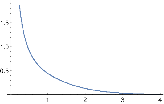
Figure 1: Effective potential of the sss-model as a function of ${\rm Im}\,T_{1}$, for ${\rm Re}\,T_{1}=0$, $U_{1}=T_{2}=U_{2}=T_{3}=U_{3}=i$. Regime (II), which corresponds to small ${\rm Im}\,T_{1}$, is connected to the super no-scale Regime (I), where ${\rm Im}\,T_{1}$ is large.

Our choice of ${\rm Re}\,T_{1}$ and $U_{1}$ is such that the curve passes through the lines $T_{1}=-1/U_{1}$ and $T_{1}/2=-\bar{U}_{1}$, when ${\rm Im}\,T_{1}=1$ and 2, respectively. However, no extremum occurs at these points. In Ref. [1], it is shown in general that in non-supersymmetric classical models, the integrated partition function at arbitrary genus-$g$ admits extrema at all “points of maximal enhanced symmetry”. The latter are the loci in moduli space where the gauge group is enhanced, with no $U(1)$ factor left. In our case, since $G^{(1)}=U(1)\times SU(2)$ and $G^{(1)}=U(1)^{2}$ at ${\rm Im}\,T_{1}=1$ and 2, there is no contradiction in not having extrema at these points. Fig. 1 shows that there exist initial conditions with $m_{3/2}$ of order $M_{\rm s}$, such that the super no-scale Regime (I) of Solution ($a$) is reached dynamically. However, as mentioned after Eq. (2.22), Wilson lines may also develop expectation values in the intermediate regime, so that the theory may end with a distinct gauge group of equal rank, or even suffer (for large deformations) from a classical tachyonic instability.

3 $T^{6}$-moduli and Wilson lines deformations

Once we have found a classical model that yields an exponentially suppressed effective potential at 1-loop, the question of the quantum stability of this background must be addressed. Actually, the worldsheet CFT admits marginal deformations, which from the spacetime point of view correspond to classical moduli. Since the 1-loop effective potential depends on these scalar deformations, the initial vacuum may be destabilized. In this section, we will study the response of the 1-loop effective potential to all worldsheet small marginal deformations, in the super no-scale regime. As an example, we consider in details the case of Background ($a$) of the sss-model but the structure of the result remains valid in any generic ${\cal N}=4\to 0$ no-scale model i.e. with $n_{\rm F}$ and $n_{\rm B}$ not necessary equal, and which is based in a gauge symmetry $U(1)^{2}\times{\cal H}$, where the rank of ${\cal H}$ is 20 and otherwise arbitrary.

3.1 Deformation of Background ($a$)

The worldsheet operators we consider are $Y_{IJ}\partial X^{I}\bar{\partial}X^{J}$ and $Y_{I{\cal I}}\partial X^{I}\bar{\partial}\bar{\phi}^{\cal I}$ for $I,J\in\{1,\dots,6\}$, ${\cal I}\in\{7,\dots,22\}$, where the $\bar{\phi}^{\cal I}$’s are the 16 extra right-moving compact bosons of the heterotic string. In Background ($a$), we have initially $T_{2}=U_{2}=T_{3}=U_{3}=i$, the gauge group is

$${\cal G}=U(1)^{2}\times SU(2)^{4}\times SO(16)^{2}\,,$$ (3.54)

and the partition function is given in Eq. (2.1), with ${\rm Im}\,T_{1}\gg 1$, $U_{1}={\cal O}(i)$. Denoting $G_{IJ}$ and $B_{IJ}$ the initial internal metric and antisymmetric tensor, $6\times 6$ real $Y$’s are introduced to define their deformed counterparts as

$$(B^{\prime}+G^{\prime})_{\alpha\beta}=(B+G)_{\alpha\beta}+\sqrt{2}\,Y_{\alpha\beta}\,,\qquad\alpha,\beta\in\{1,2\}\,,$$ (3.55)

$$(B^{\prime}+G^{\prime})_{ij}\;=\delta_{ij}+\sqrt{2}\,Y_{ij}\,,\,\quad\;\quad\qquad i,j\in\{3,4,5,6\}\,,$$ (3.56)

$$(B^{\prime}+G^{\prime})_{\alpha i}\,=\sqrt{2}\,Y_{\alpha i}\,,$$ (3.57)

$$(B^{\prime}+G^{\prime})_{i\alpha}\,=\sqrt{2}\,Y_{i\alpha}\,,$$ (3.58)

while the $6\times 16$ remaining ones,

$$Y_{\alpha{\cal I}}\,,\quad Y_{i{\cal I}}\,,\qquad\alpha\in\{1,2\}\,,\;i\in\{3,4,5,6\}\,,\;{\cal I}\in\{7,\dots,22\}\,,$$ (3.59)

are the Wilson lines of $SO(16)^{2}$ along $T^{6}$. Our goal is to determine which of the above $6\times 22$ deformations acquire at 1-loop positive squared masses or remain massless, while the leftover ones induce tachyonic instabilities.

We first derive a general expression for the 1-loop effective potential, in the regime ${\rm Im}\,T_{1}\gg 1$, $U_{1}={\cal O}(i)$. Let us consider the contribution to the 1-loop partition function arising from a single state $s$,

$$(-1)^{F}\,{1\over\tau_{2}}\,q^{{1\over 4}M_{L}^{\prime 2}/M_{\rm s}^{2}}\,\bar{q}^{{1\over 4}M_{R}^{\prime 2}/M_{\rm s}^{2}}=(-1)^{F}\,{1\over\tau_{2}}\,e^{-\pi\tau_{2}M_{L}^{\prime 2}/M_{\rm s}^{2}}\,\bar{q}^{{1\over 4}\left(M_{R}^{\prime 2}-M_{L}^{\prime 2}\right)/M_{\rm s}^{2}},$$ (3.60)

where $F$ is its fermion number. The left- and right-moving squared masses take the following form, where the “primes” mean that the expressions refer to the deformed background [26],

$$M_{L}^{\prime 2}=M_{\rm s}^{2}\Big{[}P_{I}^{\prime}\,G^{\prime-1}_{IJ}P_{J}^{\prime}+4\Big{(}N_{L}-{1\over 2}\Big{)}\Big{]},\quad M_{R}^{\prime 2}=M_{\rm s}^{2}\Big{[}\bar{P}_{I}^{\prime}\,G^{\prime-1}_{IJ}\bar{P}_{J}^{\prime}+Q^{\prime}_{\cal I}Q^{\prime}_{\cal I}+4(N_{R}-1)\Big{]},$$ (3.61)

where $N_{L},N_{R}$ denote the oscillator numbers and we have defined

$$P_{I} =m_{I}+Y_{I{\cal I}}\,Q_{\cal I}+{1\over 2}Y_{I{\cal I}}\,Y_{J{\cal I}}\,n_{J}+(B^{\prime}+G^{\prime})_{IJ}\,n_{J}\,,$$

$$\bar{P}_{I} =m_{I}+Y_{I{\cal I}}\,Q_{\cal I}+{1\over 2}Y_{I{\cal I}}\,Y_{J{\cal I}}\,n_{J}+(B^{\prime}-G^{\prime})_{IJ}\,n_{J}\,,\!\!\!\phantom{\Bigg{|}}$$

$$Q^{\prime}_{\cal I} =Q^{\prime}_{\cal I}+Y_{I{\cal I}}\,n_{I}\,.$$ (3.62)

In the above expressions, $P_{I}$ and $\bar{P}_{I}$ are generalized left- and right-moving momenta that depend on the $T^{6}$ momenta and winding numbers $m_{I}$ and $n_{I}$, while $Q_{\cal I}$, ${\cal I}\in\{7,\dots,22\}$, denote the components of a weight in a representation of the gauge group realized by the extra right-moving $\bar{\phi}^{\cal I}$’s [27]. Physically, this weight is the charge vector under $SO(16)^{2}$ of the state $s$ and its squared length is an even integer. An immediate consequence of the r.h.s. of Eq. (3.60) is that invariance under the modular translation $\tau\to\tau+1$ implies that $M_{L}^{\prime 2}-M_{R}^{\prime 2}=4L_{s}M_{\rm s}^{2}$, for some integer $L_{s}$. Therefore, $M_{L}^{\prime 2}-M_{R}^{\prime 2}$ must be invariant under the $6\times 22$ continuous deformations, a fact that is easily verified using Eqs (3.1), which yield $L_{s}=4m_{I}n_{I}-2Q_{\cal I}Q_{\cal I}+4(N_{L}-{1\over 2})-4(N_{R}-1)$.

Next, we note that for small $Y$-deformations, the term (3.60) integrated over the fundamental domain ${\cal F}$ leads a contribution of order $e^{-{\rm Im}\,T_{1}}$ to the effective potential if $s$ has non-trivial winding numbers along either of the two $1^{\rm st}$ internal directions, which are large. Therefore, we concentrate on the dominant contributions, which arise from the pure momentum states (i.e. with $2n_{1}+h=n_{2}=0$ in Eq. (2.1)). Choosing one of them, $s_{0}$, with vanishing momenta $m_{1}=m_{2}=0$ ($m_{1}\equiv 2k_{1}+g$ in Eq. (2.1)), let us gather the contributions to ${\cal V}_{\mbox{\scriptsize 1-loop}}$ of the KK towers associated to $X^{1},X^{2}$ and based on this state. In the initial Background $(a)$, one obtains

$$-{M_{\rm s}^{4}\over(2\pi)^{4}}(-1)^{F_{0}} \int_{\cal F}{d^{2}\tau\over 2\tau_{2}^{3}}\sum_{m_{1},m_{2}}(-1)^{m_{1}}\,e^{-\pi\tau_{2}{|U_{1}m_{1}-m_{2}|^{2}\over{\rm Im}\,T_{1}{\rm Im}\,U_{1}}}\,q^{{1\over 4}M_{0L}^{2}/M_{\rm s}^{2}}\,\bar{q}^{{1\over 4}M_{0R}^{2}/M_{\rm s}^{2}}$$

$$=-{M_{\rm s}^{4}\over(2\pi)^{4}}(-1)^{F_{0}}\int_{\cal F}{d^{2}\tau\over 2\tau_{2}^{4}}\,{\rm Im}\,T_{1}\sum_{\tilde{m}_{1},\tilde{m}_{2}}e^{-{\pi{\rm Im}\,T_{1}\over\tau_{2}{\rm Im}\,U_{1}}|\tilde{m}_{1}+{1\over 2}+U_{1}\tilde{m}_{2}|^{2}}\,q^{{1\over 4}M_{0L}^{2}/M_{\rm s}^{2}}\,\bar{q}^{{1\over 4}M_{0R}^{2}/M_{\rm s}^{2}}\,,$$ (3.63)

where $F_{0},M_{0L},M_{0R}$ are the fermion number and left- or right-moving masses of $s_{0}$. The insertion $(-1)^{m_{1}}$ in the l.h.s. arises from the fermion number $F=F_{0}+m_{1}$. It translates the fact that a mass splitting of order $1/{\rm Im}\,T_{1}$ exists between bosons and fermions, as follows from the spontaneous breaking of supersymmetry and can be seen in the partition function (2.1). This phase $e^{i\pi m_{1}}$ yields in the r.h.s., which is obtained by Poisson summation, a ${1\over 2}$-shift of the integer $\tilde{m}_{1}$. This shift implies that the integral in Eq. (3.1) can be extended to the full upper half-strip, $-1<\tau_{1}\leq 1$, $\tau_{2}>0$, without introducing UV divergences, and that the result differs from that obtained by integrating over ${\cal F}$ by terms of order $e^{-c\sqrt{{\rm Im}\,T_{1}}}$.

When the $Y$-deformations are switched on, $M_{0L},M_{0R}$ and more importantly the KK mass are slightly modified. The latter is initially the degree 2 polynomial in $m_{1},m_{2}$, which appears in the argument of the exponential function in the l.h.s. of Eq. (3.1), (and becomes the expression in Eq. (3.85)). However, for small enough $Y$’s, the full expression after poisson summation is still integrable over the upper half-strip (see Eq. (3.1)). It follows that the integration over $\tau_{1}$ is straightforward, implying that the surviving dominant contributions to ${\cal V}_{\mbox{\scriptsize 1-loop}}$ arise from KK states $s$ that are level-matched, $L_{s}=0$. Moreover, since the states with vanishing winding numbers along $X^{1}$ and $X^{2}$ satisfy

$$4L_{s}M_{\rm s}^{2}=M_{L}^{\prime 2}-M_{R}^{\prime 2}=M_{L}^{2}-M_{R}^{2}=M_{0L}^{2}-M_{0R}^{2}\,,$$ (3.64)

which is independent of $m_{1},m_{2}$, the whole towers of KK modes based on the level-matched states $s_{0}$ are level matched as well. Writing the associated contribution,

$$-{M_{\rm s}^{4}\over(2\pi)^{4}}(-1)^{F_{0}}\,{\rm Im}\,T_{1}\sum_{\tilde{m}_{1},\tilde{m}_{2}}\int_{0}^{+\infty}{d\tau_{2}\over 2\tau_{2}^{4}}\,e^{-{\pi{\rm Im}\,T_{1}\over\tau_{2}{\rm Im}\,U_{1}}\left[|\tilde{m}_{1}+{1\over 2}+U_{1}\tilde{m}_{2}|^{2}+{\cal O}(Y)\right]}\,e^{-\pi\tau_{2}(M_{0L}^{2}+{\cal O}(Y))/M_{\rm s}^{2}}\,,$$ (3.65)

and changing the dummy variable of integration $\tau_{2}$ into $x=\tau_{2}/{\rm Im}\,T_{1}$, we see that when the mass $M_{0L}$ of the state $s_{0}$ in the initial Background ($a$) is not vanishing, the result is exponentially suppressed. Therefore, we obtain the general expression of the 1-loop effective potential

$${\cal V}_{\mbox{\scriptsize 1-loop}}=-{M_{\rm s}^{4}\over(2\pi)^{4}}\sum_{s_{0}=1}^{n_{B}+n_{F}}(-1)^{F_{0}}\int_{0}^{+\infty}{d\tau_{2}\over 2\tau_{2}^{3}}\sum_{m_{1},m_{2}}(-1)^{m_{1}}\,e^{-\pi\tau_{2}M_{L}^{\prime 2}/M_{\rm s}^{2}}+{\cal O}\!\left(M_{\rm s}^{4}\,e^{-c\sqrt{{\rm Im}\,T_{1}}}\right)\!,$$ (3.66)

where the sum extends over the set of massless states present in the initial Background ($a$), and $M_{L}^{\prime}$ is the mass of the associated KK mode with momenta $m_{1},m_{2}$ along $X^{1},X^{2}$, once the moduli deformations are switched on.

To proceed, we resume the states $s_{0}$ of the sss-model in Background ($a$), which satisfy $M_{0L}^{2}=M_{0R}^{2}=0$. The first condition imposes $N_{L}={1\over 2}$, the second yields $N_{R}=0$ or 1, and we recall that their quantum numbers along $X^{1},X^{2}$ are $m_{1}=m_{2}=n_{1}=n_{2}=0$.

- In Sector

$$O^{(0)}_{2,2} \Big{(}O_{2,2}^{(1)}\big{[}{}^{0}_{0}\big{]}V_{8}-O_{2,2}^{(1)}\big{[}{}^{0}_{1}\big{]}S_{8}\Big{)}O^{(2)}_{2,2}\,O^{(3)}_{2,2}\,\bar{O}_{16}\bar{O}^{\prime}_{16}$$

$$={1\over\tau_{2}\,\bar{\eta}^{24}}\Big{(}\Gamma_{2,2}\big{[}{}^{0,\,0}_{0,\,0}\big{]}\!_{(T_{1},U_{1})}8-\Gamma_{2,2}\big{[}{}^{0,\,0}_{1,\,0}\big{]}\!_{(T_{1},U_{1})}8\Big{)}\Gamma_{{\rm Adj}\,SU(2)^{4}}\,\Gamma_{{\rm Adj}\,SO(16)^{2}}+{\cal O}(q\bar{q})\,,$$ (3.67)

where $\Gamma_{{\rm Adj}\,SU(2)^{4}}$ and $\Gamma_{{\rm Adj}\,SO(16)^{2}}$ are the root lattices of $SU(2)^{4}$ and $SO(16)^{2}$, we find that :

$\bullet$ At oscillator level $N_{R}=1$, 8 copies of 24 states with $F_{0}=0$ arise from the factor $8/\bar{\eta}^{24}$. They are neutral with respect to the gauge group ${\cal G}$. $8\times 2$ realize the gravity sector, while the remaining $8\times 22$ ones live in the Cartan subalgebra of ${\cal G}$. Their quantum numbers are

$$m_{i}=n_{i}=0\,,\;i\in\{3,4,5,6\}\,,\qquad Q_{\cal I}=0\,,\;{\cal I}\in\{7,\dots,22\}\,.$$ (3.68)

$\bullet$ At oscillator level $N_{R}=0$, massless states with $F_{0}=0$ arise from the $SU(2)^{4}$ enhancement of the gauge symmetry. For any given $i\in\{3,4,5,6\}$ and $\epsilon\in\{-1,1\}$, there are 8 states with quantum numbers

$$m_{i}=-n_{i}=-\epsilon\,,\quad m_{j}=n_{j}=0\,,\;j\in\{3,4,5,6\},\,j\neq i\,,\quad Q_{\cal I}=0\,,\;{\cal I}\in\{7,\dots,22\}\,.$$ (3.69)

Note that the generalized momentum $p_{R}^{i}={-1\over\sqrt{2}}(m_{i}/R_{i}-n_{i}R_{i})$ of the compact direction $X^{i}$ of radius $R_{i}=1$ is $p_{R}^{i}=\epsilon\sqrt{2}$, which is a root of squared length equal to 2 of $\Gamma_{{\rm Adj}\,SU(2)^{4}}$.

$\bullet$ Similarly, 8 copies of massless states with $F_{0}=0$ arise at oscillator level $N_{R}=0$ from the root lattice $\Gamma_{{\rm Adj}\,SO(16)^{2}}$. Their quantum numbers are

$$m_{i}=n_{i}=0\,,\;i\in\{3,4,5,6\}\,,\quad Q_{\cal I}\,,\;{\cal I}\in\{7,\dots,22\}\,\;\mbox{where}\!\!\!\phantom{\Bigg{|}}$$

$$Q_{\cal I}=\left\{\begin{array}[]{l}(\pm 1,\pm 1,0^{6};0^{8})\quad\mbox{or permutations between the entries $Q_{7}$ to $Q_{14}$,}\\ \mbox{or}\\ (0^{8};\pm 1,\pm 1,0^{6})\quad\mbox{or permutations between the entries $Q_{15}$ to $Q_{22}$.}\end{array}\right.$$ (3.73)

In the above formula, $0^{k}$ means $k$ consecutive null entries [27]. In total, there are $2\times 112$ such roots $Q_{\cal I}$ of squared lengths equal to 2.

Altogether, we recover the $n_{\rm B}=8\times(24+4\times 2+2\times 112)=8\times 256$ bosonic massless states described in Sect. 2.2.

- In Sector

$$O^{(0)}_{2,2} \Big{(}O_{2,2}^{(1)}\big{[}{}^{0}_{1}\big{]}V_{8}-O_{2,2}^{(1)}\big{[}{}^{0}_{0}\big{]}S_{8}\Big{)}O^{(2)}_{2,2}\,O^{(3)}_{2,2}\,(\bar{O}_{16}\bar{S}^{\prime}_{16}+\bar{S}_{16}\bar{O}^{\prime}_{16})$$

$$={1\over\tau_{2}\,\bar{\eta}^{24}}\Big{(}\Gamma_{2,2}\big{[}{}^{0,\,0}_{1,\,0}\big{]}\!_{(T_{1},U_{1})}8-\Gamma_{2,2}\big{[}{}^{0,\,0}_{0,\,0}\big{]}\!_{(T_{1},U_{1})}8\Big{)}\Gamma_{{\rm Spin}\,SO(16)^{2}}+{\cal O}(q\bar{q})\,,$$ (3.74)

$\Gamma_{{\rm Spin}\,SO(16)^{2}}$ is the weight lattice of the spinorial representation of $SO(16)^{2}$. 8 copies of massless states with $F_{0}=1$ occur at oscillator number $N_{R}=0$ from this lattice. Their quantum numbers are

$$m_{i}=n_{i}=0\,,\;i\in\{3,4,5,6\}\,,\quad Q_{\cal I}\,,\;{\cal I}\in\{7,\dots,22\}\,\;\mbox{where}\!\!\!\phantom{\Bigg{|}}$$

$$Q_{\cal I}=\left\{\begin{array}[]{l}(\pm 1,\pm 1,\pm 1,\pm 1,\pm 1,\pm 1,\pm 1,\pm 1;0^{8})\quad\mbox{with even number of $-1$'s,}\\ \mbox{or}\\ (0^{8};\pm 1,\pm 1,\pm 1,\pm 1,\pm 1,\pm 1,\pm 1,\pm 1)\quad\mbox{with even number of $-1$'s.}\end{array}\right.$$ (3.78)

$Q_{\cal I}$ is actually one of the $2\times 128$ weights of squared lengths equal to 2 [27]. As said in Sec. 2.2, we have a total of $n_{\rm F}=8\times(2\times 128)=8\times 256$ fermionic massless states.

We are ready to compute the contribution to the effective potential (3.66) that arises from the KK towers of states $s$ based on each of the $n_{B}+n_{F}$ states $s_{0}$, which are initially massless in Background ($a$). The momenta, winding numbers and $SO(16)^{2}$ charges of each state $s$ are those of $s_{0}$, up to the momenta $m_{1},m_{2}$ along the $X^{1},X^{2}$, which are arbitrary. We first consider the non-Cartan states of $SU(2)^{4}$. For given $i\in\{3,4,5,6\}$ and $\epsilon\in\{-1,1\}$, the contribution of $s$ to the potential involves its squared mass $M_{L}^{\prime 2}$ given in Eq. (3.61), which is expressed in terms of

$$P^{\prime}_{\alpha}=m_{\alpha}+\epsilon\Big{(}\sqrt{2}\,Y_{\alpha i}+Y_{\alpha{\cal I}}Y_{i{\cal I}}\Big{)}\,,\;\alpha\in\{1,2\}\,,\quad P^{\prime}_{j}=\epsilon\Big{(}\sqrt{2}\,Y_{ji}+Y_{j{\cal I}}Y_{i{\cal I}}\Big{)}\,,\;j\in\{3,4,5,6\}\,,$$ (3.79)

and the inverse of the metric

$$G^{\prime}_{IJ}=G_{IJ}+\sqrt{2}\,Y_{(IJ)}\qquad\mbox{where}\qquad Y_{(IJ)}={1\over 2}(Y_{IJ}+Y_{JI})\,,$$ (3.80)

which is

$$G^{\prime-1}_{IJ}=\left(\begin{array}[]{lr}\underline{G}^{-1}_{\alpha\beta}-\sqrt{2}\,\underline{G}^{-1}_{\alpha\gamma}\,Y_{(\gamma\delta)}\,\underline{G}^{-1}_{\delta\beta}+{\cal O}(Y^{2})&-\sqrt{2}\,\underline{G}^{-1}_{\alpha\gamma}\,Y_{(\gamma,k)}+{\cal O}(Y^{2})\\ \\ -\sqrt{2}\,Y_{(j\gamma)}\,\underline{G}^{-1}_{\gamma,\beta}+{\cal O}(Y^{2})&\delta_{jk}-\sqrt{2}\,Y_{(jk)}+{\cal O}(Y^{2})\end{array}\right).$$ (3.81)

In the above equation, $\underline{G}^{-1}_{\alpha\beta}$ is the inverse of the $2\times 2$ matrix $\underline{G}_{\alpha\beta}=G_{\alpha\beta}$, $\alpha,\beta\in\{1,2\}$. The contribution of the 8 copies of KK states associated to the $SU(2)^{4}$ root $i,\epsilon$ is

$${\cal V}^{i,\epsilon}_{\mbox{\scriptsize 1-loop}}=-{8\,M_{\rm s}^{4}\over 2(2\pi)^{4}}\int_{0}^{+\infty}{d\tau_{2}\over\tau_{2}^{3}} \sum_{m_{1},m_{2}}(-1)^{m_{1}}\,e^{-\pi\tau_{2}(m_{\alpha}+\xi_{\alpha})G^{\prime-1}_{\alpha\beta}(m_{\beta}+\xi_{\beta})}\;\times$$

$$\Big{[}1-2\pi\tau_{2}\,m_{\alpha}\sqrt{2}\,\underline{G}^{-1}_{\alpha\gamma}\,Y_{(\gamma j)}\,\epsilon\sqrt{2}\;Y_{ji}+{\cal O}(Y^{3})\Big{]}\,\times$$

$$\Big{[}1-\pi\tau_{2}\big{(}Y_{ji}\,\epsilon\sqrt{2}\big{)}^{2}+{\cal O}(Y^{3})\Big{]}+{\cal O}\!\left(M_{\rm s}^{4}\,e^{-c\sqrt{{\rm Im}\,T_{1}}}\right)\!\!\!\phantom{\Bigg{|}},$$ (3.82)

where $\xi_{\alpha}=\epsilon\Big{(}\sqrt{2}\,Y_{\alpha i}+Y_{\alpha{\cal I}}Y_{i{\cal I}}\Big{)}$ and we have expanded at second order in $Y$’s the $e^{-\pi\tau_{2}2P_{\alpha}^{\prime}\,G^{\prime-1}_{\alpha j}P_{j}^{\prime}}$ and $e^{-\pi\tau_{2}P_{j}^{\prime}\,G^{\prime-1}_{jk}P^{\prime}_{k}}$ contributions in the integrand. However, the $2^{\rm nd}$ line in Eq. (3.1) can be omitted, since its linear term in $m_{\alpha}$ must be dressed, at the order we are interested in, by $e^{-\pi\tau_{2}m_{\alpha}G^{-1}_{\alpha\beta}m_{\beta}}$ coming from the $1^{\rm st}$ line, and we sum over $m_{1},m_{2}$. Recalling the definition of the component $B^{\prime}_{21}$ of the deformed antisymmetric tensor and choosing the $2\times 2$ matrix $\underline{G}^{\prime-1}_{\alpha\beta}$ as follows,

$$B_{21}^{\prime}=B_{21}+{1\over\sqrt{2}}(Y_{21}-Y_{12})\,,\qquad\quad\underline{G}^{\prime-1}_{\alpha\beta}=G^{\prime-1}_{\alpha\beta}\,,\quad\alpha,\beta\in\{1,2\}\,,$$ (3.83)

we can use the inverse matrix $\underline{G}^{\prime}_{\alpha\beta}$ to define deformed moduli

$$T^{\prime}_{1}=i\sqrt{\underline{G}^{\prime}_{11}\underline{G}^{\prime}_{22}-\underline{G}_{12}^{\prime 2}}+B^{\prime}_{21}\,,\qquad\quad U^{\prime}_{1}={i\sqrt{\underline{G}^{\prime}_{11}\underline{G}^{\prime}_{2,2}-\underline{G}_{12}^{\prime 2}}+\underline{G}^{\prime}_{21}\over\underline{G}^{\prime}_{11}}\,,$$ (3.84)

in terms of which we have

$$(m_{\alpha}+\xi_{\alpha})\,G^{\prime-1}_{\alpha\beta}\,(m_{\beta}+\xi_{\beta})={|U_{1}^{\prime}(m_{1}+\xi_{1})-(m_{2}+\xi_{2})|^{2}\over{\rm Im}\,T_{1}^{\prime}\,{\rm Im}\,U_{1}^{\prime}}\,.$$ (3.85)

A Poisson summation on $m_{1},m_{2}$ in ${\cal V}^{i,\epsilon}_{\mbox{\scriptsize 1-loop}}$ then leads

$${\cal V}^{i,\epsilon}_{\mbox{\scriptsize 1-loop}}=-{8\,M_{\rm s}^{4}\over 2(2\pi)^{4}}\int_{0}^{+\infty}{d\tau_{2}\over\tau_{2}^{3}} \,{{\rm Im}\,T_{1}^{\prime}\over\tau_{2}}\sum_{\tilde{m}_{1},\tilde{m}_{2}}e^{-{\pi{\rm Im}\,T_{1}^{\prime}\over\tau_{2}{\rm Im}\,U_{1}^{\prime}}|\tilde{m}_{1}+{1\over 2}+U_{1}^{\prime}\tilde{m}_{2}|^{2}}\,e^{2i\pi{{\rm Re}\,[(\tilde{m}_{1}+{1\over 2}+U_{1}^{\prime}\tilde{m}_{2})\bar{\xi}]\over{\rm Im}\,U_{1}^{\prime}}}$$

$$\Big{[}1-\pi\tau_{2}\big{(}Y_{ji}\,\epsilon\sqrt{2}\big{)}^{2}+{\cal O}(Y^{3})\Big{]}+{\cal O}\!\left(M_{\rm s}^{4}\,e^{-c\sqrt{{\rm Im}\,T_{1}}}\right),$$ (3.86)

where $\xi=U_{1}\xi_{1}-\xi_{2}$. Expanding the phase in $\xi$ or $\bar{\xi}$ and integrating over $\tau_{2}$, one obtains the final contribution,

$${\cal V}^{i,\epsilon}_{\mbox{\scriptsize 1-loop}}= -{8\over 16\pi^{7}}\,{M_{\rm s}^{4}\over({\rm Im}\,T^{\prime}_{1})^{2}}\,E_{(1,0)}(U^{\prime}_{1}|3,0)+{8\over 16\pi^{5}}\,{M_{\rm s}^{4}\over{\rm Im}\,T_{1}}\,E_{(1,0)}(U_{1}|2,0)\;\times\!\!\!\phantom{\Bigg{|}}$$ (3.87)

$$\;\quad\qquad\qquad{1\over 2}\!\left(\sum_{j=3}^{6}\big{(}Y_{ji}\,\epsilon\sqrt{2}\big{)}^{2}+2\big{|}Y_{i}\,\epsilon\sqrt{2}\big{|}^{2}-\rho\big{(}Y_{i}\,\epsilon\sqrt{2}\big{)}^{2}-\bar{\rho}\big{(}\bar{Y}_{i}\,\epsilon\sqrt{2}\big{)}^{2}\right)\!\!\!\phantom{\underset{\hat{|}}{\Big{|}}}$$

$$\hskip 196.32384pt+{\cal O}(M_{\rm s}^{4}\,Y^{3})+{\cal O}\!\left(M_{\rm s}^{4}\,e^{-c\sqrt{{\rm Im}\,T_{1}}}\right),$$ (3.88)

where we have redefined complex moduli as

$$Y_{i}={U_{1}Y_{1i}-Y_{2i}\over\sqrt{{\rm Im}\,T_{1}{\rm Im}\,U_{1}}}\,,\qquad i\in\{3,4,5,6\}\,,$$ (3.89)

and introduced the dressing coefficient

$$\rho={E_{(1,0)}(U_{1}|2,1)\over E_{(1,0)}(U_{1}|2,0)}\,.$$ (3.90)

In Eq. (3.87), the scalars $Y_{ji}$ and $Y_{i}$, for $j\in\{3,4,5,6\}$, are actually the Wilson lines of the $i^{\rm th}$ $SU(2)$ factor along $T^{6}$, weighted by the associated root $\epsilon\sqrt{2}$.

We proceed with the contribution ${\cal V}^{Q}_{\mbox{\scriptsize 1-loop}}$ of the effective potential that arises from the KK modes $s$ based on the state $s_{0}$ of right-moving charge $Q_{\cal I}$, which is either a root of $\Gamma_{{\rm Adj}\,SO(16)^{2}}$ or a weight of $\Gamma_{{\rm Spin}\,SO(16)^{2}}$ whose length squared equals 2. The novelty is that the former have $F_{0}=0$, while the latter have $F_{0}=1$. For such a mode $s$, we have

$$P^{\prime}_{\alpha}=m_{\alpha}+Y_{\alpha{\cal I}}\,Q_{\cal I}\,,\quad\alpha\in\{1,2\}\,,\qquad\quad P^{\prime}_{j}=Y_{j{\cal I}}\,Q_{\cal I}\,,\quad j\in\{3,4,5,6\}\,.$$ (3.91)

Comparing with Eq. (3.79), we see that at second order in $Y$’s, the 8 copies of KK modes yield a contribution identical to ${\cal V}^{i,\epsilon}_{\mbox{\scriptsize 1-loop}}$, up to the overall dressing $(-1)^{F_{0}}$ and the exchanges

$$Y_{\alpha i}\,\epsilon\sqrt{2}\longrightarrow Y_{\alpha{\cal I}}\,Q_{\cal I}\,,\quad\alpha\in\{1,2\}\,,\qquad\quad Y_{ji}\,\epsilon\sqrt{2}\longrightarrow Y_{j{\cal I}}\,Q_{\cal I}\,,\quad j\in\{3,4,5,6\}\,.$$ (3.92)

Thus, we immediately conclude that

$${\cal V}^{Q}_{\mbox{\scriptsize 1-loop}}= -{(-1)^{F_{0}}\,8\over 16\pi^{7}}\,{M_{\rm s}^{4}\over({\rm Im}\,T^{\prime}_{1})^{2}}\,E_{(1,0)}(U^{\prime}_{1}|3,0)+{(-1)^{F_{0}}\,8\over 16\pi^{5}}\,{M_{\rm s}^{4}\over{\rm Im}\,T_{1}}\,E_{(1,0)}(U_{1}|2,0)\;\times\!\!\!\phantom{\Bigg{|}}$$

$$\;{1\over 2}\!\left(\sum_{j=3}^{6}\Big{(}\sum_{{\cal I}=7}^{22}Y_{j{\cal I}}\,Q_{\cal I}\Big{)}^{2}+2\Big{|}\sum_{{\cal I}=7}^{22}Y_{\cal I}\,Q_{\cal I}\Big{|}^{2}-\rho\Big{(}\sum_{{\cal I}=7}^{22}Y_{\cal I}\,Q_{\cal I}\Big{)}^{2}-\bar{\rho}\Big{(}\sum_{{\cal I}=7}^{22}\bar{Y}_{\cal I}\,Q_{\cal I}\Big{)}^{2}\right)\!\!\!\phantom{\underset{\hat{|}}{\Big{|}}}$$

$$\hskip 207.7052pt+{\cal O}(M_{\rm s}^{4}\,Y^{3})+{\cal O}\!\left(M_{\rm s}^{4}\,e^{-c\sqrt{{\rm Im}\,T_{1}}}\right),$$ (3.93)

where $Y_{j{\cal I}}$, $j\in\{3,4,5,6\}$, and

$$Y_{\cal I}={U_{1}Y_{1{\cal I}}-Y_{2{\cal I}}\over\sqrt{{\rm Im}\,T_{1}{\rm Im}\,U_{1}}}\,,\qquad{\cal I}\in\{7,\dots,22\}\,,$$ (3.94)

are the Wilson lines of $SO(16)^{2}$ along $T^{6}$.

Finally, we consider the $8\times 24$ KK towers of states that are neutral with respect to the gauge group. In this case, $F_{0}=0$ and $P^{\prime}_{\alpha},P^{\prime}_{j}$ are like those of Eq. (3.91), with $Q_{\cal I}=0$. Therefore, the effective potential contribution ${\cal V}^{e}_{\mbox{\scriptsize 1-loop}}$, for $e\in\{1,\dots,24\}$, which arises from the 8 copies of such states, is

$${\cal V}^{e}_{\mbox{\scriptsize 1-loop}}=-{8\over 16\pi^{7}}\,{M_{\rm s}^{4}\over({\rm Im}\,T^{\prime}_{1})^{2}}\,E_{(1,0)}(U^{\prime}_{1}|3,0)+{\cal O}\!\left(M_{\rm s}^{4}\,e^{-c\sqrt{{\rm Im}\,T_{1}}}\right).$$ (3.95)

In order to combine all contributions to the effective potential we have computed, we note that

$${1\over 2}\sum_{Q\in\!\!\!\!\underset{\mbox{\scriptsize of $SO(16)^{2}$}}{\mbox{\scriptsize Adjoint}}}\sum_{{\cal I}=7}^{22}A_{\cal I}Q_{\cal I}\,\sum_{{\cal J}=7}^{22}B_{\cal J}Q_{\cal J}=C({\cal A}_{SO(16)})\sum_{{\cal I}=7}^{22}A_{\cal I}B_{\cal I}\,, \!\!C({\cal A}_{SO(16)})=14\,,$$ for

$${1\over 2}\sum_{Q\in\!\!\!\underset{\mbox{\scriptsize of $SO(16)^{2}$}}{\mbox{\scriptsize Spinorial}}}\sum_{{\cal I}=7}^{22}A_{\cal I}Q_{\cal I}\,\sum_{{\cal J}=7}^{22}B_{\cal J}Q_{\cal J}=C({\cal S}_{SO(16)})\sum_{{\cal I}=7}^{22}A_{\cal I}B_{\cal I}\,, \!\!C({\cal S}_{SO(16)})=16\,,$$ for (3.96)

where $C({\rm\cal R}_{G})\delta^{ab}={\rm tr}(T^{a}T^{b})$ and $T^{a}$, $a\in\{1,\dots,\dim G\}$, are the generators in the representation ${\cal R}_{G}$ of a gauge group $G$. Given that, summing over the $4\times 2$ roots $i,\epsilon$ of $SU(2)^{4}$, the $2\times(112+128)$ charges $Q$ of $SO(16)^{2}$ and the 24 sets of neutral KK towers, one obtains the final result,

$${\cal V}_{\mbox{\scriptsize 1-loop}}= \;{n_{\rm F}-n_{\rm B}\over 16\pi^{7}}\,{M_{\rm s}^{4}\over({\rm Im}\,T^{\prime}_{1})^{2}}\,E_{(1,0)}(U^{\prime}_{1}|3,0)\!\!\!\phantom{\Bigg{|}}$$

$$\,-{3\over 16\pi^{5}}\,{M_{\rm s}^{4}\over{\rm Im}\,T_{1}}\,E_{(1,0)}(U_{1}|2,0)\Bigg{(}b_{SU(2)}\sum_{i=3}^{6}\!\bigg{[}\sum_{j=3}^{6}(Y_{ji})^{2}+2|Y_{i}|^{2}-\rho(Y_{i})^{2}-\bar{\rho}(\bar{Y}_{i})^{2}\bigg{]}\!\!\!\phantom{\underset{\hat{|}}{\Big{|}}}$$

$$\hskip 116.65646pt+b_{SO(16)}\sum_{{\cal I}=7}^{22}\!\bigg{[}\sum_{j=3}^{6}(Y_{j{\cal I}})^{2}+2|Y_{\cal I}|^{2}-\rho(Y_{\cal I})^{2}-\bar{\rho}(\bar{Y}_{\cal I})^{2}\bigg{]}\Bigg{)}\!\!\!\phantom{\underset{\hat{|}}{\Big{|}}}$$

$$\hskip 207.7052pt+{\cal O}(M_{\rm s}^{4}\,Y^{3})+{\cal O}\!\left(M_{\rm s}^{4}\,e^{-c\sqrt{{\rm Im}\,T_{1}}}\right).$$ (3.97)

In this expression, $b_{SU(2)}$ and $b_{SO(16)}$ are the $\beta$-function coefficients of each $SU(2)$ and $SO(16)$ factors,

$$b_{SU(2)} =\left(-{11\over 3}+6\times{1\over 6}\right)\!C({\cal A}_{SU(2)})=-{8\over 3}\,2\,,$$

$$b_{SO(16)} =\left(-{11\over 3}+6\times{1\over 6}\right)\!C({\cal A}_{SO(16)})+4\times{2\over 3}\,C({\cal S}_{SO(16)})$$

$$=-{8\over 3}\big{(}C({\cal A}_{SO(16)})-C({\cal S}_{SO(16)})\big{)}=-{8\over 3}\,(-2)\,,$$ (3.98)

which are obtained using the following contributions of massless degrees of freedom in the representation ${\cal R}_{G}$ of $G$,

$$b_{G}^{\mbox{\scriptsize gauge boson}}=-{11\over 3}\,C({{\cal R}_{G}})\,,\quad b_{G}^{\mbox{\scriptsize real scalar}}={1\over 6}\,C({{\cal R}_{G}})\,,\quad b_{G}^{\mbox{\scriptsize Majorana fermion}}={2\over 3}\,C({{\cal R}_{G}})\,.$$ (3.99)

Note that in the derivation of Eq. (3.1), the fact that $n_{\rm F}=n_{\rm B}$ in the sss-model plays no role. Thus, the above structure of the effective potential in terms of arbitrary $n_{\rm F}$, $n_{\rm B}$ and $\beta$-function coefficients associated to the simple gauge group factors is valid for arbitrary no-scale model realizing the ${\cal N}=4\to 0$ spontaneous breaking. In such a generic model, with $n_{\rm F}\neq n_{\rm B}$, the dominant term appearing in the $1^{\rm st}$ line in Eq. (3.1) is proportional to $m_{3/2}^{\prime 4}$, where $m_{3/2}^{\prime}$ is the deformed gravitino mass,

$$m^{\prime 2}_{3/2}={|U^{\prime}_{1}|^{2}M^{2}_{\rm s}\over{\rm Im}\,T^{\prime}_{1}\,{\rm Im}\,U^{\prime}_{1}}\,.$$ (3.100)

Observe that since the moduli $Y_{(\alpha i)}$, $\alpha\in\{1,2\}$, $i\in\{3,4,5,6\}$, are switched on, the $T^{2}\times T^{4}$ factorized form of the internal space of the initial Background ($a$) is broken, implying $m_{3/2}^{\prime}$ to depend on the whole metric of $T^{6}$. Clearly, the stability of an initial no-scale model background requires the term $m_{3/2}^{\prime 4}$ to be absent, which is nothing but the super no-scale condition $n_{\rm F}=n_{\rm B}$. If this is satisfied, we are left with the $2^{\rm nd}$ and $3^{\rm rd}$ lines in Eq. (3.1), which are proportional to $m_{3/2}^{2}M_{\rm s}^{2}$. The eigenvalues of the squared mass matrices of the dimensionful scalars $Y_{i}M_{\rm s}$, $i\in\{3,4,5,6\}$ and $Y_{\cal I}M_{\rm s}$, ${\cal I}\in\{7,\dots,22\}$ are

$$-{3b_{G}\over 16\pi^{5}}\,{M_{\rm s}^{2}\over{\rm Im}\,T_{1}}\,E_{(1,0)}(U_{1}|2,0)\big{(}1\pm|\rho|\big{)}\,,\quad\mbox{for $G=SU(2)$ or $SO(16)$}\,,$$ (3.101)

which are proportional to $m_{3/2}^{2}$, as expected for moduli not involved in the supersymmetry breaking [3]. Since $|\rho(U_{1})|<1$, Eq. (3.101) leads to the conclusion that any simple gauge group factor that is neither asymptotically free nor conformal, i.e. with $b_{G}>0$, yields to local instabilities.

In the sss-super no-scale model we consider here, the $SU(2)^{4}$ Wilson lines $Y_{ji}$ and $Y_{i}$, $j,i\in\{3,4,5,6\}$, are attracted dynamically to the origin $Y_{ji}=Y_{i}=0$, while the $SO(16)^{2}$ ones $Y_{j{\cal I}}$ and $Y_{\cal I}$, $j\in\{3,4,5,6\}$, ${\cal I}\in\{7,\dots,22\}$, condense. Due to the periodicity properties of the Wilson lines, this instability is only local and some of the $Y_{j{\cal I}}$’s and/or $Y_{\cal I}$’s are expected to develop large but finite expectation values. Note that since we started with a vanishing effective potential in the super no-scale Background ($a$), these instabilities imply that ${\cal V}_{\mbox{\scriptsize 1-loop}}$ becomes negative. We should reach another no-scale model, with new numbers of massless fermions and bosons satisfying $n^{\prime}_{\rm F}<n^{\prime}_{\rm B}$, and without non-asymptotically free gauge group factors. At this stage, the model would still be in the regime $m^{\prime}_{3/2}\ll M_{\rm s}$, which guaranties no tachyonic instability may arise. However, the scaling of the effective potential now being like $-m_{3/2}^{\prime 4}$, the gravitino mass would be dynamically attracted to larger values. Once it reaches the order of magnitude of the string scale, several scenarios may occur :

$\bullet$ A tachyon may arise at tree level, thus inducing a severe Hagedorn-like instability.

$\bullet$ $m_{3/2}$ may be stabilized at a (local) minimum, thus yielding an anti-de Sitter vacuum, where a restoration of supersymmetry may or may not occur.

$\bullet$ $m_{3/2}$ may continue increasing, with runaway behavior. The model would lead (after T-duality) to an anti-de Sitter theory in higher dimensions, explicitly non-supersymmetric.

3.2 Lifting the instabilities

In the previous sub-section we have shown the existence of two different types of instabilities. The first ones, arise in the no-scale models having $n_{\rm F}\neq n_{\rm B}$, which are due to the non-vanishing of ${\cal V}_{\mbox{\scriptsize 1-loop}}$. Actually, the vanishing of the effective potential is required by the dilaton and no-scale modulus stationary condition; namely the absence of dilaton and no-scale modulus tadpoles. The second ones are tachyonic instabilities that arise in all no-scale models having positive $\beta$-function coefficients. Therefore, it would be relevant to look for super no-scale models without non-asymptotically free gauge group factors. Possibly, one could consider no-scale models with $n_{\rm F}>n_{\rm B}$, and switch on discrete Wilson lines of order 1 in order to break the non-asymptotically free gauge group factors to products of asymptotically free and/or conformal subgroups.

Another approach is to consider the super no-scale models at finite temperature $T$. Note that this point of view can be relevant when the models are used in cosmological scenarios. At finite $T$, the effective potential is nothing but the quantum free energy and all squared masses are shifted by $T^{2}$ [23]. Thus, as long as $T^{2}$ is greater than $m_{3/2}^{2}$, the tachyonic instabilities arising from positive $\beta$-function coefficients are lifted. For instance, Background ($a$) of the sss-model is stable during early stages of the cosmological evolution, when $T$ is high. As the Universe grows and the temperature drops, the breaking of $SO(16)\times SO(16)^{\prime}$ occurs when $T^{2}$ crosses $m_{3/2}^{2}$ and becomes lower. It would be interesting to investigate this phase transition in a dynamical cosmological framework where all moduli fields, including the dilaton and the no-scale modulus, evolve with the temperature.

Another way to bypass the tachyonic instabilities occurring at 1-loop in super no-scale models may be to impose correlations among deformations, in order to preserve those which respect at the quantum level the flatness condition ${\cal V}_{\mbox{\scriptsize 1-loop}}=0$. In the case of Background ($a$), since $-b_{SU(2)}=b_{SO(16)}$, ideally the constraint

$$Y^{2}=H^{2}$$ (3.102)

may be implemented, where $Y$ is the total “attractive” Wilson line deformation associated to $SU(2)^{4}$, while $H$ is the total “repulsive” one, associated to $SO(16)^{2}$,

$$Y^{2} =\sum_{i=3}^{6}\!\bigg{[}\sum_{j=3}^{6}(Y_{ji})^{2}+2|Y_{i}|^{2}-\rho(Y_{i})^{2}-\bar{\rho}(\bar{Y}_{i})^{2}\bigg{]},$$

$$H^{2} =\sum_{{\cal I}=7}^{22}\!\bigg{[}\sum_{j=3}^{6}(Y_{j{\cal I}})^{2}+2|Y_{\cal I}|^{2}-\rho(Y_{\cal I})^{2}-\bar{\rho}(\bar{Y}_{\cal I})^{2}\bigg{]}.$$ (3.103)

Differently stated, one would demand the negative energy density created by any breaking of $SO(16)^{2}$ to be compensated by the positive one, generated by a breaking of $SU(2)^{4}$. It may be relevant to investigate this possibility by implementing additional orbifold actions.

4 ${\cal N}=2\to 0$ and ${\cal N}=1\to 0$ super no-scale models

In the super no-scale models presented so far, with exponentially suppressed vacuum energies at the 1-loop quantum level, ${\cal N}=4$ supersymmetry is spontaneously broken to ${\cal N}=0$. It is then legitimate to look for less symmetric super no-scale theories, realizing either an ${\cal N}=2\to 0$ or ${\cal N}=1\to 0$ spontaneous breaking. For this purpose, one may consider no-scale parent theories describing an ${\cal N}=4\to 0$ breaking, and implement $\mathbb{Z}_{2}$ or $\mathbb{Z}_{2}\times\mathbb{Z}_{2}$ orbifold actions that yield descendent models satisfying the super no-scale property. However, as was shown in Ref. [13], if no precautions are taken in the choice of orbifold actions, the ${\cal N}=2$ sectors of these models lead generically to gauge coupling threshold corrections [15, 16] proportional to the large internal volume [14]. In this case, a fine tuning of the string coupling $g_{\rm s}$ is required to cancel the 1-loop threshold corrections of the gauge couplings of the asymptotically free gauge group factors. In the following, we present a simple strategy that yields ${\cal N}=2\to 0$ or ${\cal N}=1\to 0$ super no-scale models, while evading the above mentioned “decompactification problem”.

4.1 Chains of ${\cal N}=4,2,1\to 0$ super no-scale models

Our goal is to derive a class of ${\cal N}=2\to 0$ and ${\cal N}=1\to 0$ super no-scale models from parent ones that realize the ${\cal N}=4\to 0$ breaking. The next subsection will describe the gauge threshold corrections arising in this case. To begin, we consider any ${\cal N}=4$ heterotic no-scale vacuum obtained by “moduli-deformed fermionic construction” [28, 13]. Let us implement a $\mathbb{Z}_{2}$ or $\mathbb{Z}_{2}\times\mathbb{Z}_{2}$ orbifold action where at least one of the $\mathbb{Z}_{2}$’s is freely acting and thus realizes a spontaneous ${\cal N}=4\to 2$ breaking. The resulting vacuum is ${\cal N}=2$ or ${\cal N}=1$ supersymmetric, which is further spontaneously broken to ${\cal N}=0$ by a stringy Scherk-Schwarz mechanism [7] realized along the $1^{\rm st}$ internal 2-torus. The latter is chosen to be large, for the supersymmetry breaking scale to be small, $m_{3/2}^{2}\propto M_{\rm s}^{2}/{\rm Im}\,T_{1}$. In total, the model describes the ${\cal N}=4\to 2\to 0$ or ${\cal N}=2\to 1\to 0$ pattern of supersymmetry breaking. To be more specific, we request the following [13] :

$\bullet$ The generator of the free $\mathbb{Z}_{2}$ action, denoted as $\mathbb{Z}^{\rm free}_{2}$, twists the coordinates of the $2^{\rm nd}$ and $3^{\rm rd}$ 2-tori, and shifts at least one of the coordinates of the $1^{\rm st}$ 2-torus, e.g.

$$\mathbb{Z}_{2}^{\rm free}\;:(X^{1},X^{2},X^{3},X^{4},X^{5},X^{6})\longrightarrow(X^{1},X^{2}+{1/2},-X^{3},-X^{4},-X^{5},-X^{6})\,.$$ (4.104)

$\bullet$ In the $\mathbb{Z}^{\rm free}_{2}\times\mathbb{Z}_{2}$ case, there is no restriction on the second $\mathbb{Z}_{2}$. However, in most cases, its generator as well as the product of the latter with the generator of $\mathbb{Z}^{\rm free}$ have fixed points. If this happens, in order not to induce large threshold corrections to the gauge couplings, we impose the $2^{\rm nd}$ and $3^{\rm rd}$ 2-tori moduli $T_{2},U_{2}$ and $T_{3},U_{3}$ not to be far from$~{}i$. For instance, they can sit at extended symmetry points.

$\bullet$ The stringy Scherk-Schwarz mechanism responsible for the final supersymmetry breaking is realized as a ${1\over 2}$-shift along the $1^{\rm st}$ 2-torus, say $X^{1}$, coupled to one of the $R$-symmetry charges, such as the helicity $a$.

Once the above restrictions are satisfied and $m_{3/2}\ll M_{\rm s}$, the effective potential of the $\mathbb{Z}_{2}^{\rm free}$ and $\mathbb{Z}^{\rm free}_{2}\times\mathbb{Z}_{2}$ models turn out to be ${1\over 2}$ and ${1\over 4}$ of that of the “parent” ${\cal N}=4\to 0$ theory, up to exponentially suppressed contributions [13],

$${\cal V}_{\mbox{\scriptsize 1-loop}}\Big{|}_{{\cal N}=4\to 2\to 0}={1\over 2}\,{\cal V}_{\mbox{\scriptsize 1-loop}}\Big{|}_{{\cal N}=4\to 0}+{\cal O}\!\left(M_{\rm s}^{4}\,e^{-cM_{\rm s}/m_{3/2}}\right),\phantom{\underset{\hat{|}}{\Big{|}}}$$

$${\cal V}_{\mbox{\scriptsize 1-loop}}\Big{|}_{{\cal N}=2\to 1\to 0}={1\over 4}\,{\cal V}_{\mbox{\scriptsize 1-loop}}\Big{|}_{{\cal N}=4\to 0}+{\cal O}\!\left(M_{\rm s}^{4}\,e^{-cM_{\rm s}/m_{3/2}c}\right).$$ (4.105)

Therefore, considering any ${\cal N}=4\to 0$ super no-scale model, such as the sss one, as a “parent” theory, one obtains automatically a chain of “descendant” models realizing the ${\cal N}=2\to 0$ or ${\cal N}=1\to 0$ breaking, with exponentially suppressed vacuum energy at 1-loop.

4.2 Threshold corrections without decompactification problem

As shown in Ref. [13], the gauge coupling threshold corrections of the $\mathbb{Z}_{2}^{\rm free}$ and $\mathbb{Z}^{\rm free}_{2}\times\mathbb{Z}_{2}$ descendant theories derived from no-scale models realizing the ${\cal N}=4\to 0$ breaking of supersymmetry turn out to have a universal form, free of decompactification problem. In the following, we present the running gauge coupling associated to a gauge group factor $G_{\alpha}$, in the $\mathbb{Z}^{\rm free}_{2}\times\mathbb{Z}_{2}$ case. At low supersymmetry breaking scale $m_{3/2}$, it is expressed in terms of moduli-dependent masses of order $m_{3/2}$ that encode the dominant contributions arising from five conformal blocks, which naturally appear in the left-moving piece of the partition function,

$$Z_{4,0}^{(\rm F)}\!\big{[}{}^{a;\,H_{1},\,H_{2}}_{b;\;G_{1},\;G_{2}}\big{]}\,S_{L}\big{[}{}^{a;\,h}_{b;\;g}\big{]}\!={1\over 2}\sum_{a,b}(-1)^{a+b+ab}\,{\theta\big{[}{}^{a}_{b}\big{]}\over\eta}\,{\theta\big{[}{}^{a+H_{2}}_{b+\,G_{2}}\big{]}\over\eta}\,{\theta\big{[}{}^{a+H_{1}}_{b\,+G_{1}}\big{]}\over\eta}\,{\theta\big{[}{}^{a-H_{1}-H_{2}}_{b\,-G_{1}-G_{2}}\big{]}\over\eta}\,(-1)^{ga+hb+hg}\,,$$ (4.106)

associated to the 8 twisted worldsheet fermions. In our conventions, $H_{1},G_{1}\in\{0,1\}$ refer to the freely acting twists of $\mathbb{Z}_{2}^{\rm free}$, while $H_{2},G_{2}\in\{0,1\}$ are those of the second $\mathbb{Z}_{2}$.

The five dominant sectors are denoted as $B$, $C$, $D$ and $I\in\{2,3\}$, and their mass threshold scales are the following [13], when no Wilson line deformations are switched on :

$$M^{2}_{B}={M^{2}_{\rm s}\over|\theta_{2}(U_{1})|^{4}\,{\rm Im}\,T_{1}\,{\rm Im}\,U_{1}}\,,\; M^{2}_{C}={M^{2}_{\rm s}\over|\theta_{4}(U_{1})|^{4}\,{\rm Im}\,T_{1}\,{\rm Im}\,U_{1}}\,,\;M^{2}_{D}={M^{2}_{\rm s}\over|\theta_{3}(U_{1})|^{4}\,{\rm Im}\,T_{1}\,{\rm Im}\,U_{1}}\,,\!\!\!\phantom{\underset{\hat{|}}{\Big{|}}}$$

$$M^{2}_{I}={M^{2}_{\rm s}\over 16\big{|}\eta(T_{I})|^{4}\,\big{|}\eta(U_{I})|^{4}\,{\rm Im}\,T_{I}\,{\rm Im}\,U_{I}},\quad I\in\{2,3\}\,.$$ (4.107)

$\bullet$ In the conformal block $B$, the supersymmetry breaking takes place, $(h,g)\neq(0,0)$, while the $\mathbb{Z}_{2}^{\rm free}\times\mathbb{Z}_{2}$ twists are trivial, $(H_{1},G_{1})=(H_{2},G_{2})=(0,0)$. It realizes the ${\cal N}=4\to 0$ spontaneous breaking.

$\bullet$ The conformal block $C$, with $(H_{1},G_{1})\neq(0,0)$ and $(h,g)=(H_{2},G_{2})=(0,0)$, preserves an ${\cal N}_{C}=2$ supersymmetry.

$\bullet$ The conformal block $D$, with $(h,g)=(H_{1},G_{1})\neq(0,0)$ and $(H_{2},G_{2})=(0,0)$, preserves an ${\cal N}_{D}=2$ supersymmetry.

In the above three sectors, the $1^{\rm st}$ 2-torus is untwisted, $(H_{2},G_{2})=(0,0)$, and its shifted lattice $\Gamma_{2,2}\big{[}{}^{\,h,\,H_{1}}_{\,g,\;G_{1}}\big{]}\!_{(T_{1},U_{1})}$ is coupled non trivially to $Z^{(F)}_{4,0}\!\big{[}{}^{a;\,H_{1},\,0}_{b;\;G_{1},\;0}\big{]}$ via the phase $S_{L}\big{[}{}^{a;\,h}_{b;\;g}\big{]}$. The mass scales $M_{B},M_{C},M_{D}$ arise from the towers of KK states along the $1^{\rm st}$ 2-torus. In the blocks $C$ and $D$, where $(H_{1},G_{1})\neq(0,0)$, the $2^{\rm nd}$ and $3^{\rm rd}$ 2-tori are twisted but the $1^{\rm st}$ one is shifted. Thus, there are no massless twisted states arising from the blocks $C$ and $D$ (no fixed points to localize them).

$\bullet$ In the remaining relevant conformal blocks $I\in\{2,3\}$, the $1^{\rm st}$ 2-torus is twisted, $(H_{2},G_{2})\neq(0,0)$. The $2^{\rm nd}$ 2-torus in untwisted for $I=2$, where $(H_{1},G_{1})=(0,0)$, while the $3^{\rm nd}$ one is untwisted for $I=3$, where $(H_{1},G_{1})=(H_{2},G_{2})$. These blocks preserve distinct ${\cal N}_{I}=2$ supersymmetries. In Eq. (4.2), the expressions of the threshold mass scales $M_{I}$’s are valid when the generator of the $2^{\rm nd}$ $\mathbb{Z}_{2}$ and its product with the generator of $\mathbb{Z}_{2}^{\rm free}$ have fixed points, namely when both $\Gamma_{2,2(T_{I},U_{I})}$ lattices are unshifted.

All other conformal blocks give either vanishing contributions, like the ${\cal N}=4$ block $A$, $(h,g)=(H_{1},G_{1})=(H_{2},G_{2})=(0,0)$, or the ${\cal N}=1$ ones, which have $\big{|}{}^{H_{1}\;\,H_{2}}_{G_{1}\;\,G_{2}}\big{|}\neq 0$. Or, their contributions are exponentially suppressed, as is the case for the blocks $E$ and $F$, which have $(H_{2},G_{2})=(0,0)$ and $\big{|}{}^{h\;\,H_{1}}_{g\;\,G_{1}}\big{|}\neq 0$, and realize ${\cal N}_{C}=2\to 0$ and ${\cal N}_{D}=2\to 0$ spontaneously broken phases.

Absorbing in a “renormalized string coupling” the universal contribution to the gauge coupling [16],

$${16\,\pi^{2}\over g_{\rm renor}^{2}} ={16\,\pi^{2}\over g_{\rm s}^{2}}-{1\over 2}Y(T_{2},U_{2})-{1\over 2}Y(T_{3},U_{3})\,,\phantom{\underset{\underset{\cdot}{\cdot}}{|}}$$

$$\mbox{with}\quad Y(T,U) ={1\over 12}\int_{\cal F}{d^{2}\tau\over\tau_{2}}\,\Gamma_{2,2}{}_{(T,U)}\left[\Big{(}\bar{E}_{2}-{3\over\pi\tau_{2}}\Big{)}{\bar{E}_{4}\bar{E}_{6}\over\bar{\eta}^{24}}-\bar{\jmath}+1008\right],$$ (4.108)

where $E_{2,4,6}=1+{\cal O}(q)$ are the holomorphic Eisenstein series of modular weights 2,4,6 and $j={1/q}+744+{\cal O}(q)$ is holomorphic and modular invariant, the final result for the running gauge coupling $g_{\alpha}(Q)$ at energy scale $Q$ is [13],

$${16\,\pi^{2}\over g_{\alpha}^{2}(Q)}=k^{\alpha}{16\,\pi^{2}\over g_{\rm renor}^{2}} -{1\over 4}b^{\alpha}_{B}\log\!\left({Q^{2}\over Q^{2}+M^{2}_{B}}\right)\!-{1\over 4}b^{\alpha}_{C}\log\!\left({Q^{2}\over Q^{2}+M^{2}_{C}}\right)\!-{1\over 4}b^{\alpha}_{D}\log\!\left({Q^{2}\over Q^{2}+M^{2}_{D}}\right)\phantom{\underset{\underset{\cdot}{\cdot}}{|}}\!\!\!\phantom{\underset{\hat{|}}{\Big{|}}}$$

$$-{1\over 2}b^{\alpha}_{2}\log\!\left({Q^{2}\over M^{2}_{2}}\right)\!-{1\over 2}b^{\alpha}_{3}\log\!\left({Q^{2}\over M^{2}_{3}}\right)+{\cal O}\!\left({m^{2}_{3/2}\over M^{2}_{\rm s}}\right).$$ (4.109)

It only depends on the Kac-Moody level $k^{\alpha}$ of the gauge group factor $G_{\alpha}$ and on 5 model-dependent $\beta$-function coefficients $b^{\alpha}_{B,C,D}$ and $b^{\alpha}_{2,3}$. The terms in the $1^{\rm st}$ line are associated to the ${\cal N}=0$, ${\cal N}_{C}=2$ and ${\cal N}_{D}=2$ spectra, which arise respectively in the conformal blocks $B$, $C$ and $D$, while those in the $2^{\rm nd}$ line arise from the ${\cal N}_{I}=2$ spectra, $I\in\{2,3\}$. Note that in the $1^{\rm st}$ line of Eq. (4.2), we have shifted $M_{B,C,D}^{2}\to Q^{2}+M_{B,C,D}^{2}$, in order to extend the validity of the result to values of $Q$ above the threshold scales $M_{B,C,D}$ at which the conformal blocks $B$, $C$ or $D$ decouple. Therefore, $Q$ is allowed to be as large as the lowest mass, which is of order $cM_{\rm s}$, of the massive states we have neglected the exponentially suppressed contributions. At low energy, i.e. $Q$ lower than the three scales $M_{B},M_{C},M_{D}$, the r.h.s. of Eq. (4.2) behaves as $-{1\over 4}(b^{\alpha}_{B}+b^{\alpha}_{C}+b^{\alpha}_{D})\log{\rm Im}\,T_{1}+{\cal O}(1)$ when ${\rm Im}\,T_{1}$ is large and $U_{1}={\cal O}(i)$. No volume term ${\cal O}({\rm Im}\,T_{1})$ being present, the models evade the decompactification problem.

As already stated in the previous subsection, up to exponentially suppressed terms, the 1-loop effective potentials in the $\mathbb{Z}_{2}^{\rm free}\times\mathbb{Z}_{2}$ models we consider here come only from the conformal block $B$ where ${\cal N}=4$ supersymmetry is spontaneously broken to ${\cal N}=0$,

$${\cal V}_{\mbox{\scriptsize 1-loop}}\Big{|}_{{\cal N}=2\to 1\to 0} ={1\over 4}\,{\cal V}_{\mbox{\scriptsize 1-loop}}\Big{|}_{{\cal N}=4\to 0}+{\cal O}\!\left(M_{\rm s}^{4}\,e^{-cM_{\rm s}/m_{3/2}}\right)\phantom{\underset{\hat{|}}{\Big{|}}}$$

$$={1\over 4}\xi(n_{\rm F}-n_{\rm B})\,m_{3/2}^{4}+{\cal O}\!\left(M_{\rm s}^{4}\,e^{-cM_{\rm s}/m_{3/2}}\right).$$ (4.110)

In this expression, $n_{\rm F}-n_{\rm B}$ is the number of massless fermions minus the number of massless bosons in the “parent” ${\cal N}=4\to 0$ theory. Actually, ${1\over 4}(n_{\rm F}-n_{\rm B})$ turns out to be the same quantity in the final ${\cal N}=1\to 0$ “descendant” model. This is a consequence of the underlying “non-aligned” ${\cal N}_{C}=2$, ${\cal N}_{D}=2$ and ${\cal N}_{I}=2$, $I\in\{2,3\}$, supersymmetries. Thus, when the initial ${\cal N}=4\to 0$ model is super no-scale, we have $n_{\rm F}-n_{\rm B}=0$, which guaranties the $\mathbb{Z}_{2}^{\rm free}$ and $\mathbb{Z}_{2}^{\rm free}\times\mathbb{Z}_{2}$ descendant orbifold theories to be super no-scale models as well.

4.3 $T^{2}\times T^{2}\times T^{2}$-moduli and Wilson lines deformations

Starting from an ${\cal N}=4\to 0$ no-scale model, the moduli space that survive $\mathbb{Z}_{2}$ or $\mathbb{Z}_{2}\times\mathbb{Z}_{2}$ orbifold actions in the “descendant” models is reduced. This follows from the fact that several deformations are frozen to some discrete values, in order to respect the factorization of the internal 6-torus as $T^{2}\times T^{4}$ or $T^{2}\times T^{2}\times T^{2}$. For instance, in the sss-model, the scalars $Y_{i}$ in Eq. (3.89) are fixed to 0. However, new moduli fields arise generically from the massless scalars of the twisted sectors. Therefore, the stability and quantum flatness condition of the ${\cal N}=2\to 0$ and ${\cal N}=1\to 0$ no-scale models must be reconsidered.

An exception however exists, for the models arising from ${\cal N}=4\to 0$ no-scale theories, on which a $\mathbb{Z}_{2}^{\rm free}$ or $\mathbb{Z}^{\rm free}_{2}\times\mathbb{Z}_{2}$ orbifold action is implemented, as described in Subsect. 4.1. In this case, modulo the constraint of the $\Gamma_{6,6}$ lattice factorization, the structure of the deformed effective potential is as in Eq. (3.1), up to the multiplicative factor ${1\over 2}$ or ${1\over 4}$, and fully arises from the untwisted sector. Due to the free action of $\mathbb{Z}_{2}^{\rm free}$, the $1^{\rm st}$ 2-torus is not fixed under any orbifold group element, so that no twisted massless states and thus no new moduli sensitive to the stringy Scherk-Schwarz mechanism is introduced. On the contrary, twisted massless states are allowed in the conformal blocks where the $2^{\rm nd}$ or $3^{\rm rd}$ 2-tori are fixed. However, being ${\cal N}_{2}=2$ or ${\cal N}_{3}=2$ supersymmetric at tree level, new moduli deformations exist, but remain exactly flat directions at 1-loop and therefore do not show up in the effective potential at this order. Thus, in the study of the quantum stability of the ${\cal N}=4\to 2\to 0$ or ${\cal N}=2\to 1\to 0$ models obtained by $\mathbb{Z}^{\rm free}$ or $\mathbb{Z}^{\rm free}_{2}\times\mathbb{Z}_{2}$ orbifold actions, only the $\beta$-function coefficients of the “parent” ${\cal N}=4\to 0$ theory are relevant. The resolution of an instability in a chain of ${\cal N}=4,2,1\to 0$ no-scale models is thus universal, in the sense that it is independent of the specific spectra of the “descendant” theories.

5 Conclusion

In this work, we focus on no-scale string models [2] where the spontaneous ${\cal N}=4,2,1\to 0$ breaking of supersymmetry is implemented at the perturbative level by geometrical fluxes. This setup realizes a “coordinate-dependent string compactification” [7, 8], in the spirit of the Scherk-Schwarz mechanism introduced in supergravity [9]. The gravitino mass scale $m_{3/2}$ is related to the inverse volume of the compact space involved in the supersymmetry breaking. Even thought supersymmetry is broken, the classical effective potential is positive semi-definite, ${\cal V}_{\rm tree}\geq 0$ [2], while the supersymmetry breaking scale $\langle m_{3/2}\rangle$ is undetermined by the flatness condition.

At the quantum level, the 1-loop effective potential receives non-trivial corrections. The latter are however under control, at least in the regime of low supersymmetry breaking scale, $m_{3/2}<cM_{\rm s}$, in which case one has

$${\cal V}_{\mbox{\scriptsize 1-loop}}=\xi(n_{\rm F}-n_{\rm B})\,m_{3/2}^{4}+{\cal O}\!\left(M_{\rm s}^{4}\,e^{-cM_{\rm s}/m_{3/2}}\right).$$ (5.111)

The above formula arises from the contributions of the light KK towers of states associated to the large internal space, and remains valid in the string context we consider even when the no-scale models realize the ${\cal N}=2\to 0$ or ${\cal N}=1\to 0$ breaking. These facts lead us to consider the situation where the numbers of massless fermionic and bosonic degrees of freedom are equal, $n_{F}=n_{B}$ [11, 12]. In this case, ${\cal V}_{\mbox{\scriptsize 1-loop}}$ vanishes modulo exponentially suppressed terms and we refer to these theories as “super no-scale string models”. At the 1-loop level, they satisfy the flatness condition, as well as the absence of dilaton and no-scale modulus tadpoles.

Simple examples of “super no-scale models” are constructed in the framework of the heterotic string compactified on $T^{2}\times T^{2}\times T^{2}$. They realize the ${\cal N}=4\to 0$ spontaneous breaking via a stringy Scherk-Schwarz mechanism along the $1^{\rm st}$ internal 2-torus and their right-moving gauge symmetry is either

$$(a)\;\;{\cal G}=U(1)^{2}\times SU(2)^{4}\times SO(16)^{2}\quad\mbox{or}\quad(b)\;\;U(1)^{3}\times SU(2)\times SU(3)\times SO(16)^{2}\,.$$ (5.112)

In both examples, if ${\cal V}_{\mbox{\scriptsize 1-loop}}$ is exponentially suppressed when $m_{3/2}<M_{\rm s}$, it is not suppressed when $m_{3/2}={\cal O}(M_{\rm s})$. However, no Hagedorn-like instability takes place in this regime [22, 8], which means that no state becomes tachyonic at any point of the $(T_{1},U_{1})$-moduli space. Moreover, in the regime where $m_{3/2}>M_{\rm s}$, the model is more naturally interpreted as an explicitly non-supersymmetric theory, rather than a no-scale model. Altogether, ${\cal V}_{\mbox{\scriptsize 1-loop}}$ turns out to be positive and increases monotonically with $m_{3/2}$. Therefore, in a cosmological context, the dynamics drives naturally these models to the super no-scale regime, where the supersymmetry breaking scale is small.

We also examine the local stability of the model with gauge symmetry ${\cal G}=U(1)^{2}\times SU(2)^{4}\times SO(16)^{2}$, under small moduli perturbations of the internal $\Gamma_{6,6+16}$ lattice. The analysis actually applies to all no-scale string models realizing an ${\cal N}=4\to 0$ breaking via stringy Scherk-Schwarz mechanism [7, 8] along a large $1^{\rm st}$ internal 2-torus, wether they are super no-scale, i.e. with $n_{\rm F}=n_{\rm B}$, or not. The rank of the gauge group being always $6+16$, we find the following three possible behaviors of the moduli $Y_{IJ}$, $I\in\{1,\dots,6\}$, $J\in\{1,\dots,6+16\}$ :

$\bullet$ For $J$ associated to a Cartan generator of an asymptotically free gauge group factor $G_{\alpha}$ ($b_{\alpha}<0$), the $Y_{IJ}$’s acquire 1-loop masses of order $m_{3/2}$, and are therefore stabilized at the origin, $Y_{IJ}=0$.

$\bullet$ For $J$ corresponding to a Cartan generator of a non-asymptotically free gauge group factor ($b_{\alpha}>0$), the $Y_{IJ}$’s aquiere negative squared masses, which leads instabilities. They condense and break $G_{\alpha}$ to subgroups with non-negative $\beta$-function coefficients.

$\bullet$ The last $Y_{IJ}$’s, associated to gauge group factors with $b_{\alpha}=0$, remain massless.

Thus, in the examples we considered, the $SO(16)\times SO(16)^{\prime}$ Wilson lines yield a destabilization of the initial background. However, we stress that in all super no-scale models, the quantum instabilities are harmless when the theories are considered at finite temperature $T$, provided that $T>m_{3/2}$. This follows from the fact that finite temperature induces effective mass terms proportional to $T^{2}(Y_{IJ})^{2}$, which screen all tachyonic contributions $-m^{2}_{3/2}(Y_{IJ})^{2}$. Therefore, in the framework of string cosmology at finite temperature [23], a phase transition happens when $T$ approaches $m_{3/2}$ from above, which drives the initial model to a new phase without non-asymptotically free gauge group factors.

A particular class of super no-scale models, which realize the spontaneous ${\cal N}=2\to 0$ or ${\cal N}=1\to 0$ breaking of supersymmetry, can be constructed easily. They are built from parent ${\cal N}=4\to 0$ super no-scale models, on which a $\mathbb{Z}^{\rm free}_{2}$ or $\mathbb{Z}^{\rm free}_{2}\times\mathbb{Z}_{2}$ orbifold action is implemented. The fact that the $\mathbb{Z}^{\rm free}_{2}$ group is freely acting ensures that the partial ${\cal N}=4\to 2$ breaking is spontaneous, which yields important consequences [13]. First, the 1-loop effective potential in the descendant models is simply $1\over 2$ or $1\over 4$ of that of the parent theory. Second, the threshold corrections to the gauge couplings are not proportional to the volume of the large internal submanifold involved in the stringy Scherk-Schwarz mechanism. This fact guaranties the validity of the string perturbative expansion, i.e. solves the so-called “decompactification problem”. In the descendent theories, the space of untwisted moduli, which are those appearing in the effective potential, is reduced, as follows from the factorization of the internal space required by the orbifold action.

To conclude, we mention that it would be very interesting to study in super no-scale models the higher order corrections in string coupling to the effective potential. This would allow to see wether insisting on the flatness condition would yield additional restrictions on the models. One can also construct super no-scale theories by implementing $\mathbb{Z}_{2}$ or $\mathbb{Z}_{2}\times\mathbb{Z}_{2}$ orbifold actions on ${\cal N}=4\to 0$ no-scale models, where each $\mathbb{Z}_{2}$ admits fixed points [11]. In this case, our analysis of the moduli deformations must be completed, since the effective potential does depend on twisted moduli sensitive to the final breaking of supersymmetry to ${\cal N}=0$. However, if these models are compatible with the physical requirement of possessing chiral spectra, the decompactification problem has to be readdressed.

References

• [1] P. H. Ginsparg and C. Vafa, “Toroidal compactification of nonsupersymmetric heterotic strings,” Nucl. Phys. B 289 (1987) 414.
• [2] E. Cremmer, S. Ferrara, C. Kounnas and D. V. Nanopoulos, “Naturally vanishing cosmological constant in ${\cal N}=1$ supergravity,” Phys. Lett.  B 133 (1983) 61;
J. R. Ellis, C. Kounnas and D. V. Nanopoulos, “Phenomenological $SU(1,1)$ supergravity,” Nucl. Phys.  B 241 (1984) 406;
J. R. Ellis, A. B. Lahanas, D. V. Nanopoulos and K. Tamvakis, “No-scale supersymmetric standard model,” Phys. Lett.  B 134 (1984) 429;
J. R. Ellis, C. Kounnas and D. V. Nanopoulos, “No scale supersymmetric GUTs,” Nucl. Phys.  B 247 (1984) 373.
• [3] S. Ferrara, C. Kounnas and F. Zwirner, “Mass formulae and natural hierarchy in string effective supergravities,” Nucl. Phys. B 429 (1994) 589 [erratum-ibid  B 433 (1995) 255] [hep-th/9405188].
• [4] H. P. Nilles, “Dynamically broken supergravity and the hierarchy problem,” Phys. Lett. B 115 (1982) 193;
H. P. Nilles, “Supergravity generates hierarchies,” Nucl. Phys. B 217 (1983) 366;
S. Ferrara, L. Girardello and H. P. Nilles, “Breakdown of local supersymmetry through gauge fermion condensates,” Phys. Lett. B 125 (1983) 457;
J. P. Derendinger, L. E. Ibanez and H. P. Nilles, “On the low-energy $d=4$, ${\cal N}=1$ supergravity theory extracted from the $d=10$, ${\cal N}=1$ superstring,” Phys. Lett. B 155 (1985) 65;
M. Dine, R. Rohm, N. Seiberg and E. Witten, “Gluino condensation in superstring models,” Phys. Lett. B 156 (1985) 55;
C. Kounnas and M. Porrati, “Duality and gaugino condensation in superstring models,” Phys. Lett. B 191 (1987) 91.
• [5] S. Gukov, C. Vafa and E. Witten, “CFT’s from Calabi-Yau four-folds,” Nucl. Phys. B 584 (2000) 69 [Nucl. Phys. B 608 (2001) 477] [hep-th/9906070];
S. B. Giddings, S. Kachru and J. Polchinski “Hierarchies from fluxes in string compactifications,” Phys. Rev. D 66 (2002) 106006 [arXiv: hep-th/0105097];
S. Kachru, M. B. Schulz, P. K. Tripathy and S. P. Trivedi, “New supersymmetric string compactifications,” JHEP 0303 (2003) 061 [arXiv:hep-th/0211182];
M. Grana, “Flux compactifications in string theory : A comprehensive review,” Phys. Rept.  423 (2006) 91 [arXiv:hep-th/0509003];
J.-P. Derendinger, C. Kounnas, P. M. Petropoulos and F. Zwirner, “Fluxes and gaugings : ${\cal N}=1$ effective superpotentials,” Fortsch. Phys.  53 (2005) 926 [hep-th/0503229];
J. P. Derendinger, C. Kounnas and P. M. Petropoulos, “Gaugino condensates and fluxes in ${\cal N}=1$ effective superpotentials,” Nucl. Phys. B 747 (2006) 190 [hep-th/0601005].
• [6] C. M. Hull, “String-string duality in ten-dimensions,” Phys. Lett.  B 357 (1995) 545 [arXiv:hep-th/9506194];
E. Witten, “String theory dynamics in various dimensions,” Nucl. Phys.  B 443 (1995) 85 [arXiv:hep-th/9503124];
J. Polchinski and E. Witten, “Evidence for heterotic - type I string duality,” Nucl. Phys.  B 460 (1996) 525 [arXiv:hep-th/9510169];
A. Dabholkar, “Ten-dimensional heterotic string as a soliton,” Phys. Lett.  B 357 (1995) 307 [arXiv:hep-th/9506160];
S. Kachru and C. Vafa, “Exact results for ${\cal N}=2$ compactifications of heterotic strings,” Nucl. Phys. B 450 (1995) 69 [hep-th/9505105];
S. Kachru, A. Klemm, W. Lerche, P. Mayr and C. Vafa, “Nonperturbative results on the point particle limit of ${\cal N}=2$ heterotic string compactifications,” Nucl. Phys. B 459 (1996) 537 [hep-th/9508155];
I. Antoniadis and H. Partouche, “Exact monodromy group of ${\cal N}=2$ heterotic superstring,” Nucl. Phys. B 460 (1996) 470 [hep-th/9509009];
I. Antoniadis, C. Bachas, C. Fabre, H. Partouche and T. R. Taylor, “Aspects of type I - type II - heterotic triality in four dimensions,” Nucl. Phys.  B 489 (1997) 160 [arXiv:hep-th/9608012];
I. Antoniadis, H. Partouche and T. R. Taylor, “Duality of ${\cal N}=2$ heterotic - type I compactifications in four dimensions,” Nucl. Phys.  B 499 (1997) 29 [arXiv:hep-th/9703076];
I. Antoniadis, H. Partouche and T. R. Taylor, “Lectures on heterotic - type I duality,” Nucl. Phys. Proc. Suppl.  61A (1998) 58; [Nucl. Phys. Proc. Suppl.  67 (1998) 3] [arXiv:hep-th/9706211];
C. Vafa and E. Witten, “Dual string pairs with ${\cal N}=1$ and ${\cal N}=2$ supersymmetry in four dimensions,” Nucl. Phys. Proc. Suppl.  46 (1996) 225 [arXiv:hep-th/9507050];
P. Kaste and H. Partouche, “On the equivalence of ${\cal N}=1$ brane worlds and geometric singularities with flux,” JHEP 0411 (2004) 033 [hep-th/0409303];
S. Kachru and E. Silverstein, “${\cal N}=1$ dual string pairs and gaugino condensation,” Nucl. Phys. B 463 (1996) 369 [hep-th/9511228];
O. Bergman and M. R. Gaberdiel, “A nonsupersymmetric open string theory and S duality,” Nucl. Phys. B 499 (1997) 183 [hep-th/9701137];
J. D. Blum and K. R. Dienes, “Strong/weak coupling duality relations for non-supersymmetric string theories,” Nucl. Phys.  B 516 (1998) 83 [arXiv:hep-th/9707160];
J. D. Blum and K. R. Dienes, “Duality without supersymmetry : The case of the $SO(16)\times SO(16)$ string,” Phys. Lett.  B 414 (1997) 260 [arXiv:hep-th/9707148];
M. Berkooz and S. J. Rey, “Nonsupersymmetric stable vacua of M theory,” JHEP 9901 (1999) 014 [Phys. Lett. B 449 (1999) 68] [hep-th/9807200].
• [7] R. Rohm, “Spontaneous supersymmetry breaking in supersymmetric string theories,” Nucl. Phys. B 237 (1984) 553;
C. Kounnas and M. Porrati, “Spontaneous supersymmetry breaking in string theory,” Nucl. Phys. B 310 (1988) 355;
S. Ferrara, C. Kounnas and M. Porrati, “Superstring solutions with spontaneously broken four-dimensional supersymmetry,” Nucl. Phys.  B 304 (1988) 500;
S. Ferrara, C. Kounnas, M. Porrati and F. Zwirner, “Superstrings with spontaneously broken supersymmetry and their effective theories,” Nucl. Phys. B 318 (1989) 75.
• [8] C. Kounnas and B. Rostand, “Coordinate dependent compactifications and discrete symmetries,” Nucl. Phys. B 341 (1990) 641.
• [9] J. Scherk and J. H. Schwarz, “Spontaneous breaking of supersymmetry through dimensional reduction,” Phys. Lett.  B 82 (1979) 60.
• [10] I. Antoniadis, “A possible new dimension at a few TeV,” Phys. Lett. B 246 (1990) 377.
• [11] S. Abel, K. R. Dienes and E. Mavroudi, “Towards a nonsupersymmetric string phenomenology,” Phys. Rev. D 91 (2015) 126014 [arXiv:1502.03087 [hep-th]].
• [12] C. Kounnas and H. Partouche, “Stringy ${\cal N}=1$ super no-scale models,” PoS PLANCK 2015 (2015) 070 [arXiv:1511.02709 [hep-th]].
• [13] A. E. Faraggi, C. Kounnas and H. Partouche, “Large volume susy breaking with a solution to the decompactification problem,” Nucl. Phys. B 899 (2015) 328 [arXiv:1410.6147 [hep-th]].
• [14] E. Kiritsis, C. Kounnas, P. M. Petropoulos and J. Rizos, “Solving the decompactification problem in string theory,” Phys. Lett. B 385 (1996) 87 [hep-th/9606087];
E. Kiritsis, C. Kounnas, P. M. Petropoulos and J. Rizos, “String threshold corrections in models with spontaneously broken supersymmetry,” Nucl. Phys. B 540 (1999) 87 [arXiv:hep-th/9807067].
• [15] V. S. Kaplunovsky, “One loop threshold effects in string unification,” Nucl. Phys. B 307 (1988) 145 [Erratum-ibid. B 382 (1992) 436] [hep-th/9205068];
L. J. Dixon, V. Kaplunovsky and J. Louis, “Moduli dependence of string loop corrections to gauge coupling constants,” Nucl. Phys. B 355 (1991) 649;
V. Kaplunovsky and J. Louis, “On gauge couplings in string theory,” Nucl. Phys. B 444 (1995) 191 [hep-th/9502077];
I. Antoniadis, K. S. Narain and T. R. Taylor, “Higher genus string corrections to gauge couplings,” Phys. Lett. B 267 (1991) 37;
P. Mayr and S. Stieberger, “Threshold corrections to gauge couplings in orbifold compactifications,” Nucl. Phys. B 407 (1993) 725 [hep-th/9303017];
E. Kiritsis and C. Kounnas, “Infrared regularization of superstring theory and the one loop calculation of coupling constants,” Nucl. Phys. B 442 (1995) 472 [hep-th/9501020];
C. Angelantonj, I. Florakis and M. Tsulaia, “Universality of gauge thresholds in non-supersymmetric heterotic vacua,” Phys. Lett. B 736 (2014) 365 [arXiv:1407.8023 [hep-th]];
C. Angelantonj, I. Florakis and M. Tsulaia, “Generalised universality of gauge thresholds in heterotic vacua with and without supersymmetry,” Nucl. Phys. B 900 (2015) 170 [arXiv:1509.00027 [hep-th]].
• [16] E. Kiritsis, C. Kounnas, P. M. Petropoulos and J. Rizos,“Universality properties of ${\cal N}=2$ and ${\cal N}=1$ heterotic threshold corrections,” Nucl. Phys. B 483 (1997) 141 [hep-th/9608034];
P. M. Petropoulos and J. Rizos, “Universal moduli dependent string thresholds in $\mathbb{Z}_{2}\times\mathbb{Z}_{2}$ orbifolds,” Phys. Lett. B 374 (1996) 49 [hep-th/9601037].
• [17] S. Kachru, J. Kumar and E. Silverstein, “Vacuum energy cancellation in a nonsupersymmetric string,” Phys. Rev. D 59 (1999) 106004 [hep-th/9807076];
S. Kachru and E. Silverstein, “On vanishing two loop cosmological constants in nonsupersymmetric strings,” JHEP 9901 (1999) 004 [hep-th/9810129];
G. Shiu and S. H. H. Tye, “Bose-Fermi degeneracy and duality in nonsupersymmetric strings,” Nucl. Phys. B 542 (1999) 45 [hep-th/9808095];
Y. Satoh, Y. Sugawara and T. Wada, “Non-supersymmetric asymmetric orbifolds with vanishing cosmological constant,” JHEP 1602 (2016) 184 [arXiv:1512.05155 [hep-th]];
Y. Sugawara and T. Wada, “More on non-supersymmetric asymmetric orbifolds with vanishing cosmological constant,” arXiv:1605.07021 [hep-th].
• [18] J. A. Harvey, “String duality and nonsupersymmetric strings,” Phys. Rev. D 59 (1999) 026002 [hep-th/9807213].
• [19] R. Blumenhagen and L. Gorlich, “Orientifolds of nonsupersymmetric asymmetric orbifolds,” Nucl. Phys. B 551 (1999) 601 [hep-th/9812158].
• [20] C. Angelantonj, I. Antoniadis and K. Forger, “Nonsupersymmetric type I strings with zero vacuum energy,” Nucl. Phys. B 555 (1999) 116 [hep-th/9904092].
• [21] K. Aoki, E. D’Hoker and D. H. Phong, “Two loop superstrings on orbifold compactifications,” Nucl. Phys. B 688 (2004) 3 [hep-th/0312181];
R. Iengo and C. J. Zhu, “Evidence for nonvanishing cosmological constant in nonSUSY superstring models,” JHEP 0004 (2000) 028 [hep-th/9912074].
• [22] J. J. Atick and E. Witten, “The Hagedorn transition and the number of degrees of freedom of string theory,” Nucl. Phys.  B 310 (1988) 291;
I. Antoniadis and C. Kounnas, “Superstring phase transition at high temperature,” Phys. Lett.  B 261 (1991) 369;
I. Antoniadis, J. P. Derendinger and C. Kounnas, “Non-perturbative temperature instabilities in ${\cal N}=4$ strings,” Nucl. Phys.  B 551 (1999) 41 [arXiv:hep-th/9902032].
• [23] T. Catelin-Jullien, C. Kounnas, H. Partouche and N. Toumbas, “Thermal/quantum effects and induced superstring cosmologies,” Nucl. Phys. B 797 (2008) 137 [arXiv:0710.3895 [hep-th]];
T. Catelin-Jullien, C. Kounnas, H. Partouche and N. Toumbas, “Induced superstring cosmologies and moduli stabilization,” Nucl. Phys. B 820 (2009) 290 [arXiv:0901.0259 [hep-th]];
F. Bourliot, C. Kounnas and H. Partouche, “Attraction to a radiation-like era in early superstring cosmologies,” Nucl. Phys. B 816 (2009) 227 [arXiv:0902.1892 [hep-th]];
F. Bourliot, J. Estes, C. Kounnas and H. Partouche, “Cosmological phases of the string thermal effective potential,” Nucl. Phys. B 830 (2010) 330 [arXiv:0908.1881 [hep-th]];
J. Estes, C. Kounnas and H. Partouche, “Superstring cosmology for ${\cal N}_{4}=1\to 0$ superstring vacua,” Fortsch. Phys.  59 (2011) 861 [arXiv:1003.0471 [hep-th]];
J. Estes, L. Liu and H. Partouche, “Massless D-strings and moduli stabilization in type I cosmology,” JHEP 1106 (2011) 060 [arXiv:1102.5001 [hep-th]];
L. Liu and H. Partouche, “Moduli stabilization in type II Calabi-Yau compactifications at finite temperature,” JHEP 1211 (2012) 079 [arXiv:1111.7307 [hep-th]].
• [24] E. Kiritsis, “String theory in a nutshell,” Princeton University Press, 2007.
• [25] C. Angelantonj, M. Cardella and N. Irges, “An alternative for moduli stabilisation,” Phys. Lett. B 641 (2006) 474 [hep-th/0608022].
• [26] E. Kiritsis and C. Kounnas, “Perturbative and nonperturbative partial supersymmetry breaking : ${\cal N}=4\to{\cal N}=2\to{\cal N}=1$,” Nucl. Phys. B 503 (1997) 117 [hep-th/9703059].
• [27] See e.g. : D. Lüst and S. Theisen, “Lectures on string theory”, Springer-Verlag, 1989.
• [28] I. Antoniadis, C. Bachas, C. Kounnas and P. Windey, “Supersymmetry among free fermions and superstrings,” Phys. Lett. B 171 (1986) 51;
I. Antoniadis, C. P. Bachas and C. Kounnas, “Four-dimensional superstrings,” Nucl. Phys. B 289 (1987) 87;
H. Kawai, D. C. Lewellen and S. H. H. Tye, “Construction of fermionic string models in four-dimensions,” Nucl. Phys. B 288 (1987) 1;
C. Kounnas and B. Rostand, “Deformations of superstring solutions and spontaneous symmetry breaking,” Hellenic School 1989:0657-668.