BPS states in the Minahan-Nemeschansky $E_{6}$ theory

Abstract

We use the method of spectral networks to compute BPS state degeneracies in the Minahan-Nemeschansky $E_{6}$ theory, on its Coulomb branch, without turning on a mass deformation. The BPS multiplicities come out in representations of the $E_{6}$ flavor symmetry. For example, along the simplest ray in electromagnetic charge space, we give the first $14$ numerical degeneracies, and the first $7$ degeneracies as representations of $E_{6}$. We find a complicated spectrum, exhibiting exponential growth of multiplicities as a function of the electromagnetic charge. There is one unexpected outcome: the spectrum is consistent (in a nontrivial way) with the hypothesis of spin purity, that if a BPS state in this theory has electromagnetic charge equal to $n$ times a primitive charge, then it appears in a spin-$\frac{n}{2}$ multiplet.

1 Introduction

1.1 Setup

The $E_{6}$ Minahan-Nemeschansky theory $T_{3}$ is a $4$-dimensional ${\mathcal{N}}=2$ superconformal field theory, first discovered in [1], and studied at great length since then (e.g. for a few highlights see [2, 3, 4, 5, 6].) In [7], it was shown that $T_{3}$ can be constructed as a theory of class $\mathcal{S}[A_{2}]$ (see [8] for more on the definition of class $\mathcal{S}$). More precisely, $T_{3}$ is the theory of class $\mathcal{S}[A_{2}]$ associated to the Riemann surface $C=\mathbb{C}\mathbb{P}^{1}\setminus\{z_{1},z_{2},z_{3}\}$ with full punctures at the points $z_{\ell}$. In this paper, we will use this description of theory $T_{3}$ extensively; indeed, we take it as our definition of $T_{3}$.

The construction of theories of class $\mathcal{S}[A_{2}]$ has in the ultraviolet a flavor symmetry group $F_{\ell}\simeq SU(3)$ for each full puncture $z_{\ell}$. In our case this gives a total flavor symmetry $F_{\mathcal{S}}\simeq SU(3)^{3}$. Remarkably, upon flowing to the infrared to reach the superconformal field theory $T_{3}$, this symmetry is enhanced to a group $F\simeq E_{6}$ (the compact simply connected form).

Theory $T_{3}$ has a 1-dimensional Coulomb branch, parameterized by $u\in\mathbb{C}$. When we move onto the Coulomb branch the scale invariance and $U(1)_{R}$ symmetry are spontaneously broken. These broken symmetries together act by $u\mapsto\lambda u$ for $\lambda\in\mathbb{C}^{\times}$. Thus the physics is the same for any $u\neq 0$. In the infrared, it is given by ${\mathcal{N}}=2$ supersymmetric $U(1)$ gauge theory. As we will explain below, the electromagnetic charge lattice $\Gamma_{\mathrm{g}}$ has three distinguished elements $\gamma_{1,2,3}$, with $\gamma_{1}+\gamma_{2}+\gamma_{3}=0$. After choosing an electromagnetic duality frame we could call one of these three “electric,” and the other two magnetic or dyonic. There is no canonical such choice, though, and indeed there is a $\mathbb{Z}_{3}$ symmetry which cyclically permutes the $\gamma_{i}$.

1.2 Summary

In this paper we compute counts of 4d BPS particles of theory $T_{3}$ on its Coulomb branch. As we have noted above, all points on the Coulomb branch are physically equivalent, so computing the counts at one point is enough to determine them everywhere on the Coulomb branch. (In particular, there are no walls of marginal stability where BPS bound states can form or decay.)

More precisely, we compute indexed counts, the second helicity supertraces $\Omega(\gamma)$, for various charges $\gamma\in\Gamma_{\mathrm{g}}$. Our main tool is the technology of spectral networks introduced in [9]. Here is a summary of the results:

1. We give an algorithm which efficiently determines $\Omega(n\gamma_{1})$, at least for $1\leq n\leq 200$. For example, we find

   $$\Omega(6\gamma_{1})=-114204.$$ (1.1)

   See §5.4 for the results with $1\leq n\leq 14$. We also give $\Omega(n(\gamma_{1}+2\gamma_{2}))$ and $\Omega(n(\gamma_{1}+3\gamma_{2}))$, both for $1\leq n\leq 13$, in §6.5.

2. We show that we have the asymptotic exponential growth

   $$\lvert\Omega(n\gamma_{1})\rvert\sim cn^{-\frac{5}{2}}(7+4\sqrt{3})^{n}$$ (1.2)

   for a constant $c$. See §5.4.

3. Since the theory $T_{3}$ has unbroken $F\simeq E_{6}$ flavor symmetry on the Coulomb branch, the $\Omega(\gamma)$ can be “upgraded” from integers to characters ${\mathbf{\Omega}}(\gamma)$ of (virtual) representations of $F\simeq E_{6}$. We compute

   • ${\mathbf{\Omega}}(n\gamma_{1})$ with $1\leq n\leq 7$,

   • ${\mathbf{\Omega}}(n(\gamma_{1}+2\gamma_{2}))$ for $1\leq n\leq 3$,

   • ${\mathbf{\Omega}}(\gamma_{1}+3\gamma_{2})$.

   See §5.4 and §6.5 for the results. For example, we find

   $${\mathbf{\Omega}}(4\gamma_{1})=-4\times\overline{\mathbf{351}}-8\times\overline{\mathbf{27}}.$$ (1.3)

   Note that we get $E_{6}$ symmetry although at intermediate stages of the computation we use a surface defect of the theory, which leaves manifest only the group $F_{\mathcal{S}}\simeq SU(3)^{3}$. This gives a check of our formalism.

4. We show that BPS states exist with all primitive charges, i.e. charges $\gamma=p\gamma_{1}+q\gamma_{2}$ with $(p,q)=1$. See §7.4.

5. Our results are consistent with a surprising hypothesis, which we call spin purity: BPS states carrying electromagnetic charges which are $n$ times a primitive charge are always in multiplets of spin $\frac{n}{2}$. (So BPS states with primitive charge are always in hypermultiplets, BPS states with 2 times the primitive charge are in vector multiplets, and so on.) For example, in (1.3) above, the multiplicities appearing are $-4$ and $-8$: these are both positive integer multiples of $-4$, which is the contribution from a spin-$2$ multiplet. See §5.3 for more on this.

Here are some open problems:

1. It would be interesting to give a direct proof within our formalism that the $SU(3)^{3}$ symmetry in the BPS indices will always be enhanced to $E_{6}$.

2. It would also be nice to prove that the BPS indices are all consistent with the spin purity hypothesis; this is true for all indices we computed, but we did not compute $\Omega(\gamma)$ for all charges.

3. Our evidence for spin purity in theory $T_{3}$ is circumstantial, because we only compute the BPS indices, which is not enough to determine the spin content uniquely. The paper [10] gives an extension of spectral network technology which can be used to compute the spin content of the BPS spectrum. Applying the methods of that paper could give a stronger check or refutation of the spin purity hypothesis in theory $T_{3}$.

4. One might wonder more generally whether spin purity is true in every superconformal field theory. (As one small piece of evidence we note that it does hold in the $SU(2)$ theory with $4$ fundamental flavors, though in a more trivial way.) Perhaps this can be proven using the same technology recently applied to the no-exotics conjecture [11].

5. The methods used in this paper in principle determine the full spectrum for all charges $\gamma\in\Gamma_{\mathrm{g}}$, including its $E_{6}$ representation content. In practice, our algorithm is rather computationally expensive, so that we have only been able to compute the degeneracies ${\mathbf{\Omega}}(\gamma)$ for a few charges. We are hopeful that with more cleverness it would be possible to obtain closed forms, or at least to compute for higher charges. This might reveal more hidden structure.

6. In Section 5.3 of [12] some BPS degeneracies are given for a five-dimensional theory, which upon $S^{1}$ compactification should reduce to the theory $T_{3}$ considered here. They appear to be related to the $\Omega(n\gamma_{1})$ we compute, but the precise relation remains an open question, as explained in §5.4 below. It would also be interesting to understand the five-dimensional meaning of the other $\Omega(\gamma)$ we compute (perhaps in terms of strings in five dimensions rather than particles.)

7. In [13], it is proposed that in a mass-deformed version of theory $T_{3}$ one can compute BPS degeneracies using quiver quantum mechanics. In particular, [13] argues that there is a point of the Coulomb branch of the mass-deformed theory where the full spectrum consists of $24$ hypermultiplets. This is far simpler than the spectrum we are finding in the massless theory. Nevertheless, using the Kontsevich-Soibelman wall-crossing formula, one could try to start from these $24$ hypermultiplets and derive the spectrum we find here; this would be a very interesting check. (We have remarked above that there are no walls in the Coulomb branch of the massless theory; however, there are plenty of walls in the larger parameter space where we include masses as well as Coulomb branch parameters.)

8. The variant of the spectral network technique which we use here should be applicable to other superconformal field theories as well. For example, it would be interesting to analyze the Minahan-Nemeschansky theories with global symmetry $E_{7}$ and $E_{8}$ [3]; this would give additional data to support or refute the spin purity conjecture.

Acknowledgements

We thank Clay Cordova, Thomas Dumitrescu, Min-xin Huang, Sheldon Katz, Albrecht Klemm, Pietro Longhi, Tom Mainiero and Chan Park for helpful discussions and comments on draft versions of this paper. LH’s work is supported by a Royal Society Dorothy Hodgkin fellowship. AN’s work is supported by National Science Foundation award 1151693.

2 Seiberg-Witten geometry

In this section we summarize the Seiberg-Witten geometry of theory $T_{3}$ and fix notation.

As for any theory of class $\mathcal{S}[A_{2}]$ with full punctures, theory $T_{3}$ has a Coulomb branch, parameterized by meromorphic cubic differentials $(\phi_{2},\phi_{3})$, such that at each puncture $\phi_{2}$ has at most a first-order pole, and $\phi_{3}$ at most a second-order pole. Using the $PSL(2,\mathbb{C})$ symmetry of $\mathbb{C}\mathbb{P}^{1}$ we can fix the punctures to be at $(z_{1},z_{2},z_{3})=(1,\omega,\omega^{2})$ with

$$\omega={\mathrm{e}}^{2\pi{\mathrm{i}}/3}.$$ (2.1)

Then the only allowed $\phi_{2}$, $\phi_{3}$ are

$$\phi_{2}=0,\qquad\phi_{3}=-\frac{u\,\mathrm{d}z^{3}}{(z^{3}-1)^{2}}.$$ (2.2)

Thus we have a $1$-dimensional Coulomb branch, parameterized by $u\in\mathbb{C}$. As we have mentioned in the introduction, the physics is the same for any $u\neq 0$; from now on we fix $u=1$.

The $U(1)$ gauge theory which appears in the infrared of theory $T_{3}$ on the Coulomb branch is naturally described in terms of the Seiberg-Witten curve,

$$\Sigma=\{\lambda^{3}+\phi_{3}=0\}\subset T^{*}C,$$ (2.3)

or more concretely, in coordinates $(x,z)$ on $T^{*}C$ where $\lambda=x\,\mathrm{d}z$,

$$\Sigma=\left\{x^{3}-\frac{1}{(z^{3}-1)^{2}}=0\right\}.$$ (2.4)

$\Sigma$ is a curve of genus $1$, with $3$ punctures. The projection $\pi:\Sigma\to C$, $\pi(x,z)=z$, is a $3$-fold covering, which is unbranched.

Filling in the punctures on $\Sigma$ we obtain a smooth compact genus $1$ curve $\overline{\Sigma}$. $\overline{\Sigma}$ is a branched covering of $\mathbb{C}\mathbb{P}^{1}$, with the branch points at the punctures. We represent this covering concretely by gluing together $3$ copies of the complex plane along branch cuts, as in Figure 2.

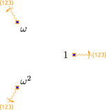
Figure 1: The thrice-punctured base curve $C=\mathbb{C}\mathbb{P}^{1}\setminus\{1,\omega,\omega^{2}\}$, in the inhomogeneous coordinate $z$. The threefold cover $\Sigma\to C$ is obtained by gluing together three sheets at branch cuts, represented by wavy orange lines. The three branch cuts meet at $z=\infty$. Each cut carries a sheet permutation $(123)$, and a coorientation labeled by an arrow, which tells us which way to do the gluing: sheet $1$ at the tail of the arrow is glued to sheet $2$ at the head of the arrow, and so on.

The $3$ sheets are labeled by the $3$ possible choices of the cube root $\lambda$ of $-\phi_{3}$. We fix the labeling as follows. At $z=0$ we have $-\phi_{3}=\mathrm{d}z^{3}$. We choose

$$\lambda^{(1)}(z=0)=\omega\,\mathrm{d}z,\qquad\lambda^{(2)}(z=0)=\omega^{2}\,\mathrm{d}z,\qquad\lambda^{(3)}(z=0)=\mathrm{d}z.$$ (2.5)

The electromagnetic charge lattice of the infrared gauge theory on the Coulomb branch is

$$\Gamma_{\mathrm{g}}=H_{1}(\overline{\Sigma},\mathbb{Z}).$$ (2.6)

As shown in Figure 2 there are $3$ distinguished charges $\gamma_{1,2,3}\in\Gamma_{\mathrm{g}}$, with $\gamma_{1}+\gamma_{2}+\gamma_{3}=0$.

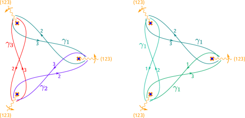
Figure 2: Cycles on $\overline{\Sigma}$. The numbers next to path segments indicate which sheet of $\overline{\Sigma}$ the segments lie on. Left: three cycles in homology classes $\gamma_{1}$, $\gamma_{2}$, $\gamma_{3}$. Right: three cycles all in the same homology class $\gamma_{1}$.

The corresponding central charges $Z_{\gamma}=\frac{1}{\pi}\oint\lambda$ are

$$Z_{\gamma_{1}}=M,\qquad Z_{\gamma_{2}}=\omega^{2}M,\qquad Z_{\gamma_{3}}=\omega M,$$ (2.7)

where

$$M =\frac{1}{\pi}\oint_{\gamma_{1}}\lambda=\frac{1}{\pi}\int_{1}^{\omega}\lambda^{(2)}+\frac{1}{\pi}\int_{\omega}^{1}\lambda^{(3)}$$ (2.8)

$$=\frac{1}{\pi}(\omega^{2}-1)\int_{1}^{\omega}\lambda^{(3)}$$ (2.9)

$$=2^{-\frac{2}{3}}\pi^{-\frac{3}{2}}\Gamma\left(\frac{1}{3}\right)\Gamma\left(\frac{1}{6}\right)\approx 1.68702.$$ (2.10)

3 Spectral networks

Our computation of the spectrum uses the technology of spectral networks, as described in [9], slightly adjusted to deal with the case of an unbroken nonabelian flavor symmetry.

For other applications of spectral networks to BPS state counting, see [14, 15, 16, 17]. Two useful tools for exploration of spectral networks are the software package loom described in Section 5.1 of [17] and the Mathematica notebook [18]. Both these tools were used in developing the picture described below.

3.1 The canonical surface defect

The key physical input to the definition of spectral networks is the canonical surface defect [19]. This is a surface defect in theory $T_{3}$, which has $C$ as its parameter space: in other words we have a family of defects $\mathbb{S}_{z}$, $z\in C$. We recall that $\mathbb{S}_{z}$ breaks the ${\mathcal{N}}=2,d=4$ supersymmetry to ${\mathcal{N}}=(2,2),d=2$. Thus we can study BPS particles living on $\mathbb{S}_{z}$ [20], whose properties are similar to those of BPS solitons in pure ${\mathcal{N}}=(2,2),d=2$ field theories [21], so we also call them “BPS solitons.” In particular these BPS solitons carry a complex-valued central charge $Z$.

The construction of $\mathbb{S}_{z}$ in the class $\mathcal{S}$ description of theory $T_{3}$ makes manifest that $\mathbb{S}_{z}$ preserves the $F_{\mathcal{S}}$ flavor symmetry. Thus we will find that the BPS solitons transform in representations of $F_{\mathcal{S}}\simeq SU(3)^{3}$. However, $\mathbb{S}_{z}$ does not need to preserve the $F\simeq E_{6}$ symmetry which appears in the infrared, and indeed we will find below that the BPS solitons on $\mathbb{S}_{z}$ do not transform in representations of $F$. Of course, the BPS states of the 4d theory $T_{3}$ do transform in representations of $F$, as we will verify in the examples we compute below.

3.2 Spectral networks

Now we recall the notion of spectral network. There is one spectral network $\mathcal{W}(\vartheta)\subset C$ for each phase $\vartheta$. A point $z\in C$ lies on $\mathcal{W}(\vartheta)$ if and only if $\mathbb{S}_{z}$ carries BPS solitons of central charge $Z$, such that $-Z$ has phase $\vartheta$. In this case we will say that $z\in C$ supports these BPS solitons. In general $\mathcal{W}(\vartheta)$ is made up of curves called walls, each wall corresponding to a single soliton charge.

In [9] an algorithm was described for determining $\mathcal{W}(\vartheta)$. The key idea is first to restrict attention to solitons which are lighter than some mass cutoff $\Lambda$, thus defining a truncated network $\mathcal{W}(\vartheta)[\Lambda]$. For very small $\Lambda$ (much lighter than the masses of any BPS particles in the $4$-dimensional theory), $\mathcal{W}(\vartheta)[\Lambda]$ is contained in the union of small neighborhoods around the points where some solitons become massless. There is a standard generic behavior around a point $z$ where only a single soliton becomes massless, which we can use to determine $\mathcal{W}(\vartheta)[\Lambda]$ for very small $\Lambda$. Then there is a scheme for determining how $\mathcal{W}(\vartheta)[\Lambda]$ evolves as $\Lambda$ is continuously increased: each wall ends at a “tip” where the soliton mass reaches $\Lambda$, and the walls grow from their tips, according to a differential equation expressing the condition that ${\mathrm{e}}^{-{\mathrm{i}}\vartheta}Z$ remains real. When walls cross, additional walls can be born from the intersection points, corresponding to bound states formed between existing solitons. See [9] for the details. Taking the limit $\Lambda\to\infty$ produces the desired $\mathcal{W}(\vartheta)$.

For the purpose of studying 4d BPS states of charge $\gamma$, we need to study the spectral network corresponding to the phase

$$\vartheta_{\gamma}=\arg(-Z_{\gamma}).$$ (3.1)

Note that $\vartheta_{\gamma}=\vartheta_{n\gamma}$ for any $n>0$, so the single network $\mathcal{W}(\vartheta_{\gamma})$ contains information about 4d BPS states with all charges $\gamma,2\gamma,3\gamma,\dots$.

In the simple examples computed in [9], each spectral network was only responsible for finitely many 4d BPS states. However, in [22] it was found that in ${\mathcal{N}}=2$ super Yang-Mills with gauge group $SU(3)$, a single network can give rise to infinitely many 4d BPS states (though still finitely many with each fixed charge). We will see below that this also happens in theory $T_{3}$.

3.3 Spectral networks in theory $T_{3}$

Because of the unbroken flavor symmetry in the 4-dimensional theory $T_{3}$, the networks $\mathcal{W}(\vartheta)$ have some special features. In particular, when $z$ approaches any of the punctures $z_{\ell}$ on $C$, several solitons on $\mathbb{S}_{z}$ become massless at once. In this situation, the rules of [9] cannot be applied directly to determine $\mathcal{W}(\vartheta)$.

Nevertheless, we can determine the shape of $\mathcal{W}(\vartheta)$ by first making a small deformation of theory $T_{3}$ by a mass parameter $m$, taking instead of (2.2)

$$\phi_{2}=\frac{mz\,\mathrm{d}z^{2}}{(z^{3}-1)^{2}},\qquad\phi_{3}=-\frac{\mathrm{d}z^{3}}{(z^{3}-1)^{2}}.$$ (3.2)

This deformation breaks the flavor symmetry to a Cartan subgroup. After making this perturbation, the rules of [9] can be applied to determine the network $\mathcal{W}(\vartheta)$. Then we can determine $\mathcal{W}(\vartheta)$ in the massless theory by taking the limit $m\to 0$. We will see an example momentarily.

3.4 The circle network

To make our discussion more concrete, we now specialize to a specific phase, $\vartheta=\pi$. This will lead to a particularly simple spectral network $\mathcal{W}(\vartheta)$. Since $\vartheta_{\gamma_{1}}=\pi$ this is the phase relevant for studying BPS states of charge $n\gamma_{1}$, $n>0$. In §6 below, we will consider more general charges and networks.

We begin by studying $\mathcal{W}(\vartheta)$ for $\vartheta$ slightly perturbed from $\pi$. Figure 3.4 shows a sample network $\mathcal{W}(\vartheta)[\Lambda]$, obtained with the help of a computer and the Mathematica notebook [18].

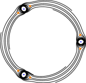
Figure 3: The spectral network $\mathcal{W}(\vartheta=\pi+0.02)[\Lambda=1.5]$, where we took $m=1.25$ in (3.2). The blue dots are the punctures, and the orange crosses are branch points of the deformed spectral cover $\Sigma$.

Looking at Figure 3.4, we notice immediately that it is “almost degenerate,” in the sense that there are groups of walls which are close together. The reason for this is that there are various solitons whose electromagnetic charges differ by some multiple of $\gamma_{1}$; their central charges thus differ by a real number (in fact an integer multiple of $M$). In the limit where we take $\vartheta\to\pi$, the walls supporting these solitons merge into a single wall, which now supports infinitely many distinct solitons, with masses diverging to $\infty$. In Figure 3.4 we show the behavior very near $\vartheta=\pi$.

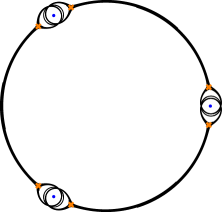
Figure 4: The spectral network $\mathcal{W}(\vartheta=\pi+0.002)[\Lambda=1.5]$, where we took $m=1.25$ in (3.2). The blue dots are the punctures, and the orange crosses are branch points of the deformed spectral cover $\Sigma$.

Then taking the mass deformation $m\to 0$, the figure is further simplified, because the branch points move onto the punctures. Thus we arrive at the network of Figure 3.4. It consists of three walls connecting the three punctures. The three walls together make up the equator of $C$.

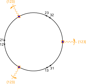
Figure 5: The spectral network $\mathcal{W}(\vartheta=\pi)$.

The labels $ij$ on each wall in Figure 3.4 tell us which types of BPS solitons can occur there. We call a soliton “of type $ij$” if it interpolates between the vacuum of $\mathbb{S}_{z}$ labeled $i$ (at $x\to-\infty$) and the vacuum labeled $j$ (at $x\to+\infty$). If $z$ is on a wall of $\mathcal{W}(\vartheta=\pi)$ carrying the label $ij$, then there exists a BPS soliton of type $ij$ on $\mathbb{S}_{z}$ with central charge $Z\in\mathbb{R}_{+}$. As we move $z$ along a wall of $\mathcal{W}(\vartheta=\pi)$, the central charge of these BPS solitons changes, while remaining real and positive. The arrow next to a label $ij$ in Figure 3.4 indicates the direction in which the central charge is increasing, for solitons of type $ij$.

As we see from Figure 3.4, each of the three walls in $\mathcal{W}(\vartheta=\pi)$ is supporting solitons of two complementary types, $ij$ and $ji$. We call walls which support two complementary types of solitons “double walls” (previously “two-way streets” in the parlance of [9].)

4 Computing the soliton spectrum

4.1 Counting BPS solitons

We now consider the spectrum of BPS solitons supported on the defect $\mathbb{S}_{z}$, when $z$ lies on $\mathcal{W}(\vartheta=\pi)$. Actually, if we take precisely $\vartheta=\pi$ this spectrum is ill-defined, due to mixing with BPS states of the bulk 4-dimensional theory carrying charge $n\gamma_{1}$. This mixing is precisely what we want to study, as an indirect way of determining the spectrum of bulk BPS states. So what we do (again following the rules of [9]) is to study not $\vartheta=\pi$ on the nose but rather the two limits $\vartheta\to\pi^{\pm}$. These correspond to two “resolutions” of the network, as shown in Figure 4.1. In each of the two resolutions, each double wall is split into two infinitesimally separated walls.

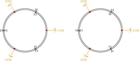
Figure 6: The two resolutions of the spectral network $\mathcal{W}(\vartheta=\pi)$.

As we have explained, in general there can be multiple solitons with $Z\in\mathbb{R}_{+}$ on the same $\mathbb{S}_{z}$. The Hilbert space $\mathcal{H}_{z}$ of BPS solitons on the defect $\mathbb{S}_{z}$ is decomposed into sectors $\mathcal{H}_{z,ij}$, where $i,j$ label the asymptotic vacua at spatial infinity. In addition, different solitons in $\mathcal{H}_{z,ij}$ can carry different electromagnetic charges, which we label $a$. Thus $\mathcal{H}_{z,ij}$ is decomposed into charge sectors $\mathcal{H}_{z,ij,a}$.

The electromagnetic charges $a$ of the solitons are not integrally quantized: rather, they have a fractional part, determined by the parameter $z$ of the surface defect as well as the vacua $i$, $j$ connected by the soliton, as explained in [20]. Still, we may have different solitons with the same values of $i,j,z$ and in this case their electromagnetic charges do differ by a quantized charge as usual. The invariant way of describing this is to say that the charges $a\in\Gamma_{ij,zz}$ where $\Gamma_{ij,zz}$ is a torsor for the lattice $\Gamma_{\mathrm{g}}$. Concretely, $\Gamma_{ij,zz}$ can be identified with the set of homology classes of open paths on $\overline{\Sigma}$, running from $z^{(i)}$ to $z^{(j)}$. The central charge of a soliton with charge $a$ is

$$Z=Z_{a}=\frac{1}{\pi}\int_{a}\lambda$$ (4.1)

where $\lambda\in\Omega^{1,0}(\Sigma)$ is the tautological 1-form.

We count the BPS solitons by a supersymmetric index depending on a flavor parameter $g\in F_{\mathcal{S}}\simeq SU(3)^{3}$:

$$\mu_{z,ij,a}(g)=\operatorname{Tr}_{\mathcal{H}_{z,ij,a}}F(-1)^{F}g.$$ (4.2)

When $g=1$ this reduces to the index considered in [21]; short multiplets of ${\mathcal{N}}=(2,2)$ supersymmetry ($2$ states) contribute $\pm 1$ to this index depending on whether the ground state has fermion number $F$ even or odd; long multiplets ($4$ states) contribute $0$. For general $g$, we use the decomposition of $\mathcal{H}_{z,ij,a}$ as a direct sum of multiplets $V\otimes W$, where $V$ is a representation of $F_{\mathcal{S}}$ and $W$ a representation of ${\mathcal{N}}=(2,2)$ supersymmetry; if $W$ is short the multiplet $V\otimes W$ contributes $\pm\operatorname{Tr}_{V}g$, and if $W$ is long it contributes $0$.

It is convenient to package the spectrum into a formal generating function:

$$\mathbf{S}_{z}=\sum_{a\in\Gamma_{ij,zz}}\mu_{z,ij,a}X_{a},$$ (4.3)

where $X_{a}$ is a formal variable, obeying the multiplicative relation $X_{b}X_{a}=X_{a+b}$ if $a$ and $b$ are paths which can be concatenated as in Figure 4.1, and $X_{a}X_{b}=0$ otherwise.

Figure 7: Two paths $a$, $b$ on $\Sigma$ which can be concatenated; the concatenated path is $a+b$.

The generating functions $\mathbf{S}_{z}$ for different points $z$, $z^{\prime}$ on the same wall are related to one another by “continuation” or “Gauss-Manin connection”: as we continuously deform $z$ to $z^{\prime}$, the paths $a\in\Gamma_{ij,zz}$ continuously deform into paths $a^{\prime}\in\Gamma_{ij,z^{\prime}z^{\prime}}$, and the degeneracies $\mu_{z,ij,a}$ remain constant. More formally, we can describe this as follows. Let $I$ denote the wall segment running from $z$ to $z^{\prime}$, and let $I^{-1}$ be the reverse of $I$. Let $\mathbf{F}_{I}$ denote the sum of the $3$ lifts of $I$ to $\Sigma$,

$$\mathbf{F}_{I}=\sum_{i=1}^{3}X_{I^{(i)}}.$$ (4.4)

and similarly $\mathbf{F}_{I^{-1}}$. Then

$$\mathbf{S}_{z^{\prime}}=\mathbf{F}_{I}\mathbf{S}_{z}\mathbf{F}_{I^{-1}}.$$ (4.5)

4.2 Framed 2d-4d BPS states

The constraints which we use to determine the $\mathbf{S}_{z}$ arise from consideration of yet another kind of BPS states, the framed 2d-4d BPS states attached to supersymmetric interfaces between surface defects $\mathbb{S}_{z}$ and $\mathbb{S}_{z^{\prime}}$ [20].

Given a path $\wp$ on $C$ between $z$ and $z^{\prime}$ and a phase $\vartheta$, there is a corresponding supersymmetric interface $\mathbb{L}_{\wp,\vartheta}$. Since we are fixing $\vartheta=\pi$ until §6, we abbreviate this as $\mathbb{L}_{\wp}$. The framed 2d-4d BPS states on $\mathbb{L}_{\wp}$ make up a Hilbert space $\mathcal{H}_{\wp}$, which decomposes similarly to the Hilbert space $\mathcal{H}_{z}$ we considered above. First, $\mathcal{H}_{\wp}$ decomposes into sectors $\mathcal{H}_{\wp,ij}$ labeled by the asymptotic vacua $ij$. Second, $\mathcal{H}_{\wp,ij}$ decomposes into sectors $\mathcal{H}_{\wp,ij,a}$ labeled by the possible 4d electromagnetic charges $a\in\Gamma_{ij,zz^{\prime}}$ where $\Gamma_{ij,zz^{\prime}}$ is the space of homology classes of open paths on $\overline{\Sigma}$, running from $z^{(i)}$ to $z^{\prime(j)}$. Finally, $\mathcal{H}_{\wp,ij,a}$ is a representation of the flavor symmetry $F_{\mathcal{S}}\simeq SU(3)^{3}$. We count the framed 2d-4d BPS states by a supersymmetric index which is a function on $F_{\mathcal{S}}$:

$${\overline{\underline{\Omega}}}_{\wp,ij,a}(g)=\operatorname{Tr}_{\mathcal{H}_{\wp,ij,a}}(-1)^{F}g.$$ (4.6)

It is convenient to package the spectrum into a generating function

$$\mathbf{F}_{\wp}=\sum_{i,j=1}^{3}\mathbf{F}_{\wp,ij},\qquad\mathbf{F}_{\wp,ij}=\sum_{a\in\Gamma_{ij,zz^{\prime}}}{\overline{\underline{\Omega}}}_{\wp,ij,a}X_{a}$$ (4.7)

where the $X_{a}$ are formal variables as above.

4.3 Constraints on framed 2d-4d BPS states

The spectrum of framed 2d-4d BPS states on interfaces $\mathbb{L}_{\wp}$ obeys constraints which are easily summarized in terms of the corresponding $\mathbf{F}_{\wp}$:

1. If $\wp$ and $\wp^{\prime}$ are two paths which are homotopic, then

   $$\mathbf{F}_{\wp}=\mathbf{F}_{\wp^{\prime}}.$$ (4.8)

2. If $\wp$ and $\wp^{\prime}$ are two paths which can be concatenated, so that the end of $\wp^{\prime}$ equals the start of $\wp$, then

   $$\mathbf{F}_{\wp\wp^{\prime}}=\mathbf{F}_{\wp}\mathbf{F}_{\wp^{\prime}}.$$ (4.9)

3. If $\wp$ is a path which does not cross any of the walls, then

   $$\mathbf{F}_{\wp}=\sum_{i=1}^{3}X_{\wp^{(i)}}$$ (4.10)

   where $\wp^{(i)}$ denote the $3$ lifts of the path $\wp$ to $\Sigma$.

4. If $\wp$ is a path which crosses just a single wall, then

   $$\mathbf{F}_{\wp}=\mathbf{F}_{\wp_{-}}(1\pm\mathbf{S}_{z})\mathbf{F}_{\wp_{+}},$$ (4.11)

   where $\wp_{\pm}$ are the two segments of $\wp$ as shown in Figure 4, and $z$ is the intersection point.

   

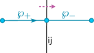
   Figure 8: The path $\wp$ crossing a wall, divided into two segments $\wp_{\pm}$. The dotted arrow indicates a choice of coorientation of the wall.

   The sign $\pm$ in (4.11) is controlled by a subtle point which we have suppressed until now: in general there are ambiguities in defining the fermion number operator $F$ which appears in the definition of $\mu$. In [9] a scheme for fixing these ambiguities was proposed, and we assume here that this scheme is correct; this means that to fix the ambiguity we need to choose a coorientation of each wall in $\mathcal{W}$. The sign in (4.11) is $+$ if we cross in the direction given by the coorientation, and $-$ if we cross in the opposite direction. In Figure 4 the dotted arrow indicates one possible choice of coorientation; for this choice the sign in (4.11) would be $+$.

5. Let $\wp$ be a loop which goes counterclockwise around puncture $z_{\ell}$. Let $\mathbf{M}_{\wp}(g)$ denote the matrix $\{\mathbf{F}_{\wp,ij}(g)\}_{i,j=1}^{3}$. Then $\operatorname{Tr}\mathbf{M}_{\wp}(g)$ is a linear combination of the formal variables $X_{a}$ for $a\in\Gamma_{ii,zz}$. Passing from $a\in\Gamma_{ii,zz}$ to the corresponding class $\gamma\in\Gamma_{\mathrm{g}}$ (“forgetting” the basepoint $z^{(i)}$) we replace these formal variables by formal variables $X_{\gamma}$, $\gamma\in\Gamma_{\mathrm{g}}$, now lying in a commutative algebra, with the simple relation $X_{\gamma}X_{\gamma^{\prime}}=X_{\gamma+\gamma^{\prime}}$. In particular $X_{\gamma=0}$ behaves as the identity, so we write $X_{\gamma=0}=1$.

   Now we can formulate our condition around the puncture. First, it says that only the trivial element $X_{\gamma=0}$ occurs in $\operatorname{Tr}\mathbf{M}_{\wp}(g)$. Since $X_{\gamma=0}=1$ this means we can interpret $\operatorname{Tr}\mathbf{M}_{\wp}(g)$ simply as a number. Second, the condition says that this number is fixed, as follows. Let $R_{\ell}$ denote a $3$-dimensional representation of the flavor symmetry group $F_{\mathcal{S}}=F_{1}\times F_{2}\times F_{3}$, in which $F_{\ell}\simeq SU(3)$ acts via the fundamental representation ${\mathbf{3}}$, and the other two $F_{\ell^{\prime}}$ act trivially. Then:

   $$\operatorname{Tr}\mathbf{M}_{\wp}(g)=\operatorname{Tr}_{R_{\ell}}g,\qquad\operatorname{Tr}\mathbf{M}_{\wp}(g)^{-1}=\operatorname{Tr}_{\overline{R}_{\ell}}g.$$ (4.12)

   These two conditions together are equivalent to requiring that the characteristic polynomial of $\mathbf{M}_{\wp}(g)$ equals the characteristic polynomial of $g$ acting in representation $R_{\ell}$.

4.4 The constraint equations

Perhaps surprisingly, the constraints of §4.3 are strong enough to determine all of the soliton generating functions $\mathbf{S}_{z}$. To see how this works, we first consider the local picture we obtain by zooming in around one of the punctures on the left side of Figure 4.1. This picture is indicated in Figure 4.4.

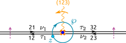
Figure 9: The local picture around one of the punctures on the left side of Figure 4.1.

More precisely, this is the picture for the puncture at $z=\omega$; for the other punctures we would act by a cyclic permutation on the sheet labels $123$. This permutation does not affect any of the following computations.

We have labeled the walls in Figure 4.4 with the symbols $\tau_{1},\tau_{2},\nu_{1},\nu_{2}$ which we use to represent the $\mathbf{S}_{z}$ on these four walls. In Figure 4.4 we have also marked a loop $\wp$ on $C$, beginning and ending at the marked point $z$. According to the constraints of §4.3, we have

$$\mathbf{F}_{\wp}=\mathbf{F}_{\wp_{-}}(1-\nu_{2})(1-\tau_{2})\mathbf{F}_{\wp_{+}}(1+\nu_{1})(1+\tau_{1}).$$ (4.13)

Here the $\nu$’s and $\tau$’s are evaluated at the places where $\wp$ crosses the walls. $\mathbf{F}_{\wp_{+}}$ is the sum of three terms for the three lifts of $\wp_{+}$ to $\Sigma$, and likewise $\mathbf{F}_{\wp_{-}}$:

$$\mathbf{F}_{\wp_{-}}=x_{11}+x_{22}+x_{33},\qquad\mathbf{F}_{\wp_{+}}=x_{13}+x_{21}+x_{32},$$ (4.14)

where each $x_{ij}=X_{a}$ for $a$ a path beginning on sheet $i$ and ending on sheet $j$.

Thus we can write

$$\mathbf{M}_{\wp}=\\ \begin{pmatrix}x_{11}&0&0\\ 0&x_{22}&0\\ 0&0&x_{33}\end{pmatrix}\begin{pmatrix}1&0&0\\ 0&1&0\\ 0&-\nu_{2}&1\end{pmatrix}\begin{pmatrix}1&0&0\\ 0&1&-\tau_{2}\\ 0&0&1\end{pmatrix}\begin{pmatrix}0&x_{21}&0\\ 0&0&x_{32}\\ x_{13}&0&0\end{pmatrix}\begin{pmatrix}1&\nu_{1}&0\\ 0&1&0\\ 0&0&1\end{pmatrix}\begin{pmatrix}1&0&0\\ \tau_{1}&1&0\\ 0&0&1\end{pmatrix}\\ =\begin{pmatrix}x_{11}x_{21}\tau_{1}&x_{11}x_{21}&0\\ -x_{22}\tau_{2}x_{13}(1+\nu_{1}\tau_{1})&-x_{22}\tau_{2}x_{13}\nu_{1}&x_{22}x_{32}\\ x_{33}(1+\nu_{2}\tau_{2})x_{13}(1+\nu_{1}\tau_{1})&x_{33}(1+\nu_{2}\tau_{2})x_{13}\nu_{1}&-x_{33}\nu_{2}x_{32}\end{pmatrix}.$$ (4.15)

This formula is hard to read because of the proliferation of $x_{ij}$’s. Fortunately, we can safely set all $x_{ij}=1$, at the cost of remembering that $x_{ij}$ may need to be inserted to make the products well defined and nonzero; there is always a unique way of doing so. From now on we adopt this convention. Then we can replace (4.15) by the simpler

$$\mathbf{M}_{\wp}=\begin{pmatrix}\tau_{1}&1&0\\ -\tau_{2}(1+\nu_{1}\tau_{1})&-\tau_{2}\nu_{1}&1\\ (1+\nu_{2}\tau_{2})(1+\nu_{1}\tau_{1})&(1+\nu_{2}\tau_{2})\nu_{1}&-\nu_{2}\end{pmatrix}.$$ (4.16)

This gives for the characteristic polynomial

$$P(t)=1+t(\nu_{1}-\tau_{2}+\nu_{2}\tau_{1})+t^{2}(-\nu_{2}-\tau_{2}\nu_{1}+\tau_{1})-t^{3}.$$ (4.17)

According to constraint 5 of §4.3, this is supposed to be equal to

$$P(t)=\prod_{k=1}^{3}(\xi_{k}^{-1}-t)=1-At+Bt^{2}-t^{3},$$ (4.18)

where $\xi_{k}\in\mathbb{C}^{\times}$ are the $3$ eigenvalues of $g$ in representation $R_{\ell}$, satisfying $\prod_{k=1}^{3}\xi_{k}=1$, and we defined $A=\sum_{k=1}^{3}\xi_{k}$, $B=\sum_{k=1}^{3}\xi_{k}^{-1}$. Comparing (4.17) and (4.18) determines the “outgoing” $\tau_{n}$ in terms of the “incoming” $\nu_{n}$:

$$\tau_{1}=\frac{B+A\nu_{1}+\nu_{1}^{2}+\nu_{2}}{1-\nu_{1}\nu_{2}},\qquad\tau_{2}=\frac{A+B\nu_{2}+\nu_{2}^{2}+\nu_{1}}{1-\nu_{1}\nu_{2}},$$ (4.19)

where the denominator is to be expanded in a geometric series. These equations are the key to computing all the soliton counts, as we will see momentarily.

4.5 A decoupled limit

It is interesting to consider what (4.19) would imply if we assume that both $\nu_{n}=0$. In this case we just get

$$\tau_{1}=B,\qquad\tau_{2}=A.$$ (4.20)

In other words, each of the two outgoing walls supports $3$ solitons, transforming in either the ${\bf 3}$ or $\overline{\bf 3}$ of the flavor symmetry $F_{\ell}\simeq SU(3)$. We might also write this as

$$\tau_{1}=\overline{\bf 3},\qquad\tau_{2}={\bf 3}.$$ (4.21)

Thus the situation is as in Figure 4.5.

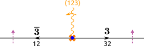
Figure 10: The spectral network and soliton counts in a neighborhood of a puncture $z_{\ell}$, including their transformation under the flavor symmetry $F_{\ell}\simeq SU(3)$, if we assume that there are no walls incoming.

This result has a direct physical interpretation. In the limit $z\to z_{\ell}$, the central charges for some of the BPS solitons on the surface defect $\mathbb{S}_{z}$ go to zero. If we concentrate just on this light sector, $\mathbb{S}_{z}$ appears to be a 2d theory decoupled from the 4d bulk, namely the supersymmetric sigma model into $\mathbb{C}\mathbb{P}^{2}$. Indeed, the soliton spectrum of this model precisely consists of the ${\bf 3}\oplus{\overline{\bf 3}}$ of the $SU(3)$ flavor symmetry [26].

We can also see these $3+3$ solitons directly as follows. We make a mass perturbation of the theory and zoom in on a small neighborhood of one of the punctures. The mass deformation splits the puncture into a puncture and two branch points. A local model for the situation is obtained by taking the puncture at $z=0$ and

$$\phi_{2}=\frac{3m^{2}}{z^{2}}\mathrm{d}z^{2},\qquad\phi_{3}=\frac{2{\mathrm{i}}}{z^{2}}\mathrm{d}z^{3}.$$ (4.22)

The branch points are at $\Delta=4\phi_{2}^{3}+27\phi_{3}^{2}=0$, i.e. $z=\pm m^{3}$. Now we consider a small perturbation of the phase $\vartheta$ away from $\vartheta=\pi$. The resulting spectral network, determined using the Mathematica notebook [18], looks like Figure 4.5.

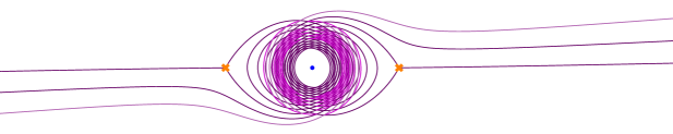
Figure 11: A spectral network $\mathcal{W}(\vartheta=\pi+0.015)[\Lambda=32]$, in the theory corresponding to the differentials (4.22) with $m=1$. The empty region around $z=0$ comes from the truncation to solitons of mass $<\Lambda$. The colors of walls indicate their genealogy: lighter walls are born from the intersections of darker ones.

Since we have perturbed to a generic phase, each wall in Figure 4.5 supports only one soliton charge. The three walls headed to the left are carrying the ${\bf\overline{3}}$ while the three headed to the right are carrying the ${\bf 3}$. In the massless limit $m\to 0$, the flavor symmetry is restored, and the three walls on each side merge into a single wall carrying the whole multiplet. Moreover, in this limit all the complexity in the middle of Figure 4.5 gets squashed into a single point, the massless puncture; thus the picture reduces to Figure 4.5.

A similar analysis was carried out in [15] Section 4.3, which considered a full puncture in a different $\mathcal{S}[A_{2}]$ theory but reached the same conclusion that this puncture emits two triplets of walls (under (4.20) of that paper.)

The basic phenomenon that walls of the spectral network can emanate from a puncture, and carry multiplets of the flavor symmetry at the puncture, is not limited to the case of theory $T_{3}$; we expect to find it generically in theories of class $\mathcal{S}$ with nonabelian flavor symmetries. (See also [8] Section 3.2.9 and [15] for related discussion.) It would be interesting to explore more systematically the landscape of possible punctures and what kind of walls they emit. (In the case of theories of class $\mathcal{S}[A_{1}]$ the answer is simple: there is only one type of regular puncture, and when its $SU(2)$ flavor symmetry is unbroken it emits a single wall, carrying the representation ${\bf 2}$. This can be verified by an analysis very similar to what we have done here.)

4.6 The actual solutions

In the actual situation of our interest, we do not have $\nu_{n}=0$: rather, from Figure 4.1 and Figure 4.4 it follows that each $\nu_{n}$ for a given puncture is related to a $\tau_{n}$ for a neighboring puncture, since each “incoming” wall is also “outgoing” from a neighboring puncture. Reintroducing the index $\ell\in\{1,2,3\}$ to keep track of the punctures (recall $z_{1}=1,z_{2}=\omega,z_{3}=\omega^{2}$) this gives the relations

$$\nu_{1,\ell}=x\tau_{2,\ell+1},\quad\nu_{2,\ell}=x\tau_{1,\ell-1},$$ (4.23)

where the factors $x=X_{\gamma_{1}}$ arise from the “continuation” discussed in §4.1. Using (4.23) to eliminate the $\nu_{n,\ell}$ from (4.19), we obtain a system of $6$ algebraic equations for $6$ unknown functions $\tau_{n,\ell}(x,\{A_{\ell}\},\{B_{\ell}\})$:

$$\tau_{1,\ell}=\frac{B_{\ell}+A_{\ell}x\tau_{2,\ell+1}+x^{2}\tau_{2,\ell+1}^{2}+x\tau_{1,\ell-1}}{1-x^{2}\tau_{2,\ell+1}\tau_{1,\ell-1}},\qquad\tau_{2,\ell}=\frac{A_{\ell}+B_{\ell}x\tau_{1,\ell-1}+x^{2}\tau_{1,\ell-1}^{2}+x\tau_{2,\ell+1}}{1-x^{2}\tau_{2,\ell+1}\tau_{1,\ell-1}}.$$ (4.24)

The full solutions to these equations seem to be rather unwieldy. If we specialize for a moment to the case $g=1$, i.e. all $A_{\ell}=B_{\ell}=3$, then we obtain a simple solution which can be written explicitly: all $\tau_{n,\ell}$ are equal and given by

$$\tau_{n,\ell}=\frac{1-x-\sqrt{1-14x+x^{2}}}{2x}=3+12x+84x^{2}+732x^{3}+7140x^{4}+\cdots$$ (4.25)

Note in particular the leading $3$, which matches the $3$ light solitons from §4.5. All the other terms represent heavier solitons.

(4.25) is not the only solution to (4.24) with $g=1$, but it is the only one which has a small-$x$ expansion given by a series in nonnegative powers of $x$, and thus it is the one which gives the actual soliton spectrum.

5 Computing the bulk BPS states

After this detour to compute BPS soliton spectra on the surface defects $\mathbb{S}_{z}$, we return to the question we really wanted to answer: what is the spectrum of BPS particles of charge $n\gamma_{1}$ in the four-dimensional theory $T_{3}$?

5.1 The flavorless spectrum

Let us begin by computing the BPS indices at $g=1$: this corresponds to forgetting their transformation under flavor symmetry. We follow the recipe laid out in Sections 6.3 and 6.4 of [9]. (This recipe was derived using the “halo picture” which expresses how jumps of the spectrum of 2d-4d BPS states are controlled by the spectrum of pure 4d BPS states; thus the $\Omega(\gamma)$ are determined indirectly from the jump of the $\mathbf{F}_{\wp}$ when $\vartheta$ crosses the critical phase $\vartheta_{\gamma}$. For our present purposes, it will be enough to know what the recipe is, without delving into its derivation.)

Let $p$ denote one of the three walls of the unresolved spectral network (Figure 3.4). According to [9], we must consider a product which combines contributions from the solitons on the two constituent walls after resolving:

$$Q(p)=1+\tau\nu.$$ (5.1)

(In this case the $Q(p)$ for all three $p$ are the same.) Then we must decompose this product in the form

$$Q(p)=\prod_{n=1}^{\infty}(1-(-x)^{n})^{\alpha_{n}(p)}.$$ (5.2)

Using (4.23), (4.25) to determine $\tau$, $\nu$ we have

$$Q(p) =1+x\left(\frac{1-x-\sqrt{1-14x+x^{2}}}{2x}\right)^{2}$$ (5.3)

$$=1+x(3+12x+84x^{2}+732x^{3}+7140x^{4}+\cdots)^{2}$$ (5.4)

$$=1+9x+72x^{2}+648x^{3}+6408x^{4}+67464x^{5}+\cdots$$ (5.5)

$$=(1+x)^{9}(1-x^{2})^{-36}(1+x^{3})^{240}(1-x^{4})^{-2160}(1-x^{5})^{21600}\cdots$$ (5.6)

from which we read off

$$(\alpha_{n}(p))_{n=1}^{\infty}=9,-36,240,-2160,21600,\dots$$ (5.7)

Now, the recipe of [9] says that we can compute the second helicity supertrace $\Omega(n\gamma)$ from the $\alpha_{n}(p)$ as follows. Each double wall $p$ lifts to a chain $p_{\Sigma}$ on $\Sigma$. We are to compute the cycle

$$L(n\gamma)=\sum_{p}\alpha_{n}(p)p_{\Sigma}.$$ (5.8)

The homology class $[L(n\gamma)]$ is a multiple of $\gamma$, and then

$$\Omega(n\gamma)=[L(n\gamma)]/(n\gamma).$$ (5.9)

In our situation we are taking $\gamma=\gamma_{1}$, each $p_{\Sigma}$ is separately closed and has $[p_{\Sigma}]=\gamma_{1}$, and all three $\alpha_{n}(p)$ are equal, so (5.8), (5.9) collapse to the simple formula

$$\Omega(n\gamma_{1})=\frac{3}{n}\alpha_{n}.$$ (5.10)

Using (5.7), this gives

$$(\Omega(n\gamma_{1}))_{n=1}^{\infty}=27,-54,240,-1620,12960,\dots$$ (5.11)

These are our first BPS counts.

5.2 The flavorful spectrum

The result (5.11) is encouraging: $\Omega(\gamma_{1})=27$ looks good for a theory which is supposed to have flavor symmetry $F\simeq E_{6}$, since the BPS states should be in a representation of $F$, and the smallest nontrivial representations of $E_{6}$ have dimension $27$! We might similarly guess that $\Omega(2\gamma_{1})=-54$ means the states of charge $2\gamma_{1}$ are in two $27$-dimensional representations, and that $\Omega(3\gamma_{1})=240$ means three copies of the $78$-dimensional adjoint plus six copies of the $1$-dimensional trivial representation.

As we go to larger $n$ it gets increasingly difficult to guess the correct $E_{6}$ representations underlying $\Omega(n\gamma_{1})$. Fortunately we do not have to guess; we just need to compute the BPS indices at general $g\in F_{\mathcal{S}}$, instead of at $g=1$. We write these indices as ${\mathbf{\Omega}}(\gamma_{1})$. Since $F_{\mathcal{S}}$ and $F$ have the same rank, knowing the transformation of the BPS states under $F_{\mathcal{S}}$ is sufficient to determine the full $F$ representation content.

When $g\neq 1$ we have not found an exact closed-form expression for the $\tau_{n,\ell}$. As a matter of principle, though, there is no problem in using (4.24), together with the assumption that the small-$x$ limit is finite, to determine $\tau_{n,\ell}$ to any finite order in the $x$ expansion. At each order we get some polynomial in the variables $A_{\ell},B_{\ell}$. For example, expanding to order $x$ gives

$$\tau_{1,\ell} =B_{\ell}+x(A_{\ell}A_{\ell+1}+B_{\ell-1})+\cdots$$ (5.12)

$$\tau_{2,\ell} =A_{\ell}+x(B_{\ell}B_{\ell-1}+A_{\ell+1})+\cdots$$ (5.13)

As above we can then compute for each wall $p_{\ell}$

$$Q(p_{\ell}) =1+\tau_{1,\ell}\nu_{1,\ell}$$ (5.14)

$$=1+x\tau_{1,\ell}\tau_{2,\ell+1}$$ (5.15)

$$=1+x(B_{\ell}A_{\ell+1})+x^{2}(B_{\ell}^{2}B_{\ell+1}+B_{\ell}A_{\ell+2}+A_{\ell}A^{2}_{\ell+1}+A_{\ell+1}B_{\ell-1})+\cdots$$ (5.16)

The next step is to expand each $Q(p)$ as a product, of the form

$$Q(p)=\prod_{n=1}^{\infty}\prod_{\lambda\in\Lambda}(1-(-x)^{n}\lambda)^{\alpha_{n,\lambda}(p)}$$ (5.17)

where $\Lambda\simeq\mathbb{Z}^{6}$ denotes the character lattice of $F_{\mathcal{S}}$. We collect these into characters

$${\boldsymbol{\alpha}}_{n}(p)=\sum_{\lambda\in\Lambda}\alpha_{n,\lambda}(p)\lambda,$$ (5.18)

and then generalizing (5.8) we define

$${\mathbf{L}}(n\gamma)=\sum_{p}{\boldsymbol{\alpha}}_{n}(p)p_{\Sigma}.$$ (5.19)

${\mathbf{L}}(n\gamma)$ is a “character-valued $1$-cycle” on $\Sigma$, i.e. a $1$-cycle whose coefficients are characters of $F_{\mathcal{S}}$ instead of integers. ${\mathbf{L}}(n\gamma)$ is necessarily a multiple of $[\gamma]$, and the BPS index we are after is the coefficient:

$${\mathbf{\Omega}}(n\gamma)=[{\mathbf{L}}(n\gamma)]/(n\gamma).$$ (5.20)

Here we are taking $\gamma=\gamma_{1}$, and (as in the flavorless case above) all $p_{\Sigma}$ are separately closed and have $[p_{\Sigma}]=\gamma_{1}$. Then (5.20) reduces to

$${\mathbf{\Omega}}(n\gamma_{1})=\frac{1}{n}\sum_{\ell=1}^{3}{\boldsymbol{\alpha}}_{n}(p_{\ell})$$ (5.21)

generalizing (5.9).

For example, we get in this way

$${\mathbf{\Omega}}(\gamma_{1})=\sum_{\ell=1}^{3}{\boldsymbol{\alpha}}_{1}(p_{\ell})=B_{1}A_{2}+B_{2}A_{3}+B_{3}A_{1}.$$ (5.22)

If we substitute $A_{\ell}=B_{\ell}=3$ as before, we recover $\Omega(\gamma_{1})=27$. More generally, from (5.22) we see that ${\mathbf{\Omega}}(\gamma_{1})$ is the character of a specific representation of $F_{\mathcal{S}}\simeq SU(3)^{3}$:

$${\mathbf{\Omega}}(\gamma_{1})=({\bf\overline{3}},{\bf 3},{\bf 1})+({\bf 1},{\bf\overline{3}},{\bf 3})+({\bf 3},{\bf 1},{\bf\overline{3}}).$$ (5.23)

Since the flavor symmetry is enhanced from $F_{\mathcal{S}}$ to $F\simeq E_{6}$, we expect that this representation should arise by decomposing some representation of $E_{6}$, and indeed this is the case: (5.23) matches the decomposition of the irreducible representation $\bf{\overline{27}}$. (Our conventions for $E_{6}$ representations are given in Appendix A.) We summarize this by writing:

$${\mathbf{\Omega}}(\gamma_{1})=\bf{\overline{27}}.$$ (5.24)

The formula (5.24) does not quite determine the spectrum of BPS particles with charge $\gamma_{1}$, because of the usual possibility of cancellations in the index. The simplest possibility would be that the spectrum consists of BPS hypermultiplets transforming in the representation $\bf{\overline{27}}$.

A similar but longer computation leads to the result

$${\mathbf{\Omega}}(2\gamma_{1})=-2\times{\mathbf{27}},$$ (5.25)

i.e. $-2$ times the character of the representation ${\mathbf{27}}$. Recalling that a BPS vector multiplet contributes $-2$ to $\Omega$, the simplest possibility is that the spectrum of BPS particles of charge $2\gamma_{1}$ consists of BPS vector multiplets in the $\bf{27}$.

Continuing in this way we obtain at the next few orders

$${\mathbf{\Omega}}(3\gamma_{1}) =3\times{\mathbf{78}}+6\times{\mathbf{1}},$$ (5.26)

$${\mathbf{\Omega}}(4\gamma_{1}) =-4\times{\mathbf{\overline{351}}}-8\times{\mathbf{\overline{27}}}.$$ (5.27)

5.3 Spin purity

Looking at the data (5.24), (5.25), (5.26), (5.27), a surprising phenomenon emerges: in ${\mathbf{\Omega}}(n\gamma_{1})$ all the multiplicities are positive integer multiples of $(-1)^{n+1}n$. In other words, if for primitive $\gamma$ we define the reduced index

$${\mathbf{\Omega}}_{\mathrm{red}}(n\gamma)=\frac{{\mathbf{\Omega}}(n\gamma)}{(-1)^{n+1}n},$$ (5.28)

then what we have seen is that ${\mathbf{\Omega}}_{\mathrm{red}}(n\gamma_{1})$ is the character of an actual (not virtual) representation of $F\simeq E_{6}$. Below we will see that this is also true up to $n\leq 7$, and we will see the same phenomenon for several other primitive charges $\gamma$.

It would be very interesting to understand why this is the case. One attractive possibility is that there is a kind of spin purity in this theory: all of the BPS particles of charge $n\gamma$ are in multiplets with spin $\frac{n}{2}$. Each such multiplet contributes $(-1)^{n+1}n$ to ${\mathbf{\Omega}}(n\gamma)$, so if spin purity indeed occurs, then we can interpret ${\mathbf{\Omega}}_{\mathrm{red}}(n\gamma)$ simply as the count of spin-$\frac{n}{2}$ multiplets.

We note that spin purity does not occur in arbitrary ${\mathcal{N}}=2$ theories: for example, it was shown in [22] that in the ${\mathcal{N}}=2$ supersymmetric pure $SU(3)$ Yang-Mills theory, there is a point on the Coulomb branch where the spectrum of BPS particles with fixed charge involves multiplets of many different spins.

On the other hand, spin purity does occur in the superconformal ${\mathcal{N}}=2$ supersymmetric $SU(2)$ Yang-Mills with $4$ hypermultiplet flavors, on its Coulomb branch. Indeed, in that theory, along each ray in the electromagnetic charge lattice, we have a primitive charge $\gamma$, and the BPS spectrum consists of $8$ hypermultiplets of charge $\gamma$ plus $1$ vector multiplet of charge $2\gamma$. This example is much simpler than theory $T_{3}$, since it involves no BPS particles with spin $>1$, and correspondingly no BPS particles of charge $n\gamma$ for $n>2$.

With all this in mind, we can formulate a hypothesis: perhaps spin purity occurs in every ${\mathcal{N}}=2$ superconformal theory on its Coulomb branch. A weaker hypothesis would be that spin purity occurs in every ${\mathcal{N}}=2$ superconformal theory for which the Coulomb branch is $1$-dimensional.

5.4 Multiplicities at higher charge

With computer assistance we computed ${\mathbf{\Omega}}(n\gamma_{1})$ up to $n=7$, with the following results:

$n$	${\mathbf{\Omega}}_{\mathrm{red}}(n\gamma_{1})$
$1$	$\overline{\mathbf{27}}$
$2$	${\mathbf{27}}$
$3$	${\mathbf{78}}+2\times{\mathbf{1}}$
$4$	${\mathbf{\overline{351}}}+2\times{\mathbf{\overline{27}}}$
$5$	${\mathbf{1728}+2\times\mathbf{351}+6\times\mathbf{27}}$
$6$	${\mathbf{5824}+\mathbf{2430}+2\times\mathbf{2925}+6\times\mathbf{650}+13\times\mathbf{78}+16\times\mathbf{1}}$
$7$	${\overline{\mathbf{19305}}}+3\times{\overline{\mathbf{17550}}}+6\times{\overline{\mathbf{7371}}}+13\times{\overline{\mathbf{1728}}}+12\times{\overline{\mathbf{351^{\prime}}}}+29\times{\overline{\mathbf{351}}}+44\times{\overline{\mathbf{27}}}$

With our current algorithms we were not able to go higher than $n=7$ while keeping all the flavor information. If we discard the flavor information, though, we can easily use the results of §5.1 to compute up to $n=200$; the first few results are:

$n$	$\Omega_{\mathrm{red}}(n\gamma_{1})$
$1$	$27$
$2$	$27$
$3$	$80$
$4$	$405$
$5$	$2592$
$6$	$19034$
$7$	$154224$
$8$	$1344357$
$9$	$12387408$
$10$	$119234916$
$11$	$1188951696$
$12$	$12206381574$
$13$	$128421415008$
$14$	$1379545102782$

We close this section with two remarks about these numbers:

• It is interesting to compare these results with those of Section 5.3 of [12], where BPS degeneracies are given for a five-dimensional theory obtained by compactifying $M$-theory on the cone over a del Pezzo surface $dP_{6}$. Upon $S^{1}$ compactification, this theory should reduce to the theory $T_{3}$ considered here. The counts given in [12] are nonnegative integers depending on a single electric charge $n$ with $1\leq n\leq 7$, and two spins $j_{L},j_{R}\in\frac{1}{2}\mathbb{Z}$. If we simply sum up those counts over $j_{L}$ and $j_{R}$, i.e. compute the total number of spin multiplets, the result agrees with the $\Omega_{\mathrm{red}}(n\gamma_{1})$ computed here, for $1\leq n\leq 6$. For $n=7$, however, there is a mismatch: summing up the degeneracies given in the last table of Section 5.3 in [12] gives $156438$, while the table above gives $154224$. Moreover, this mismatch appears to persist for all $n\geq 7$.

  The agreement for $1\leq n\leq 6$ looks unlikely to be a coincidence, but we have not understood it: Why is the total number of spin multiplets the right thing to compare? Why does a mismatch appear at $n\geq 7$? Relations between 4d and 5d BPS states have been proposed before in the literature; see particularly [29, 30]. Those papers concern gravitational theories rather than pure field theories, but perhaps some relative of their constructions can explain the agreement (and disagreement) we have found.

• From a glance at the table one sees immediately that $\Omega(n\gamma)$ grows exponentially with $n$. The phenomenon of exponential growth of BPS spectra in sufficiently complicated ${\mathcal{N}}=2$ theories has been noted before, e.g. in [22, 31, 32].

  To study this growth more quantitatively, we use a strategy recently employed in [31]: we note that the function $Q(x)$ which appeared in (5.3) obeys the algebraic equation

  $$xQ^{2}-(x^{2}-6x+1)Q+(x+1)^{2}=0.$$ (5.29)

  In particular, the discriminant of (5.29) is

  $$\Delta=(x^{2}-6x+1)^{2}-4x(x+1)^{2}=(x-1)^{2}(x^{2}-14x+1)$$ (5.30)

  which vanishes at

  $$x_{*}=(7+4\sqrt{3})^{-1}.$$ (5.31)

  Meanwhile, (5.29) says $Q(x)$ can vanish only at $x=-1$. Thus the Taylor series expansion of $\log Q(x)$ around $x=0$ is convergent up to $\lvert x\rvert=(7+4\sqrt{3})^{-1}$, and hence its coefficients grow as $\approx(7+4\sqrt{3})^{n}$. As explained in [31], this is the same as the growth of the coefficients $\Omega(n\gamma_{1})$ of the plethystic logarithm; moreover the methods of [31] allow us to determine the subleading power-law behavior:

  $$\lvert\Omega(n\gamma_{1})\rvert\sim cn^{-\frac{5}{2}}(7+4\sqrt{3})^{n},$$ (5.32)

  for some constant $c$. This indeed matches well with the data.

6 Other charges

So far we have discussed BPS counts $\Omega(\gamma)$ and ${\mathbf{\Omega}}(\gamma)$ where $\gamma$ is a multiple of $\gamma_{1}$. All of these BPS counts were computed using the single spectral network $\mathcal{W}(\vartheta=\pi)$. More generally, we can study BPS states with any charge $\gamma\in\Gamma_{\mathrm{g}}$, at the cost of having to consider more intricate spectral networks. In this section we briefly discuss these more general charges.

6.1 Charges and phases

Fix a charge

$$\gamma_{[p,q]}=p\gamma_{1}+q\gamma_{2}\in\Gamma_{\mathrm{g}}.$$ (6.1)

Then using (2.7) we have

$$Z_{\gamma_{[p,q]}}=(p+\omega^{2}q)M.$$ (6.2)

Thus BPS states of charge $\gamma_{[p,q]}$ have mass

$$M_{\gamma_{[p,q]}}=\lvert Z_{\gamma_{[p,q]}}\rvert=\lvert p+\omega^{2}q\rvert M=M\sqrt{p^{2}+q^{2}-pq}.$$ (6.3)

To study BPS states of charge $\gamma_{[p,q]}$, we need to draw the spectral network at

$$\vartheta_{[p,q]}=\arg(-Z_{\gamma_{[p,q]}})$$ (6.4)

i.e.

$$\tan\vartheta_{[p,q]}=\frac{\sqrt{3}q}{q-2p},\qquad\vartheta_{[p,q]}\in\begin{cases}(0,\pi)&\text{ if }q>0,\\ (-\pi,0)&\text{ if }q<0,\end{cases}\qquad\begin{tabular}[]{cc}$\vartheta_{[1,0]}=\pi$,&$\vartheta_{[-1,0]}=0$,\\ $\vartheta_{[1,2]}=\frac{\pi}{2}$,&$\vartheta_{[-1,-2]}=-\frac{\pi}{2}$.\end{tabular}$$ (6.5)

6.2 Symmetries

The networks

$$\mathcal{W}(\vartheta_{[p,q]}),\qquad\mathcal{W}(\vartheta_{[-p,-q]})$$ (6.6)

differ only by reversal of the sheet labels on each wall, and their phases differ by $\pi$. It follows that $\Omega(\gamma_{[p,q]})=\Omega(\gamma_{[-p,-q]})$. This kind of charge-conjugation symmetry is a general feature of all ${\mathcal{N}}=2$ theories.

More nontrivially, the residual $\mathbb{Z}_{3}$ symmetry on the Coulomb branch of theory $T_{3}$ is also reflected in a symmetry between spectral networks:

$$\mathcal{W}(\vartheta_{[p,q]}),\qquad\mathcal{W}(\vartheta_{[q-p,-p]}),\qquad\mathcal{W}(\vartheta_{[-q,p-q]})$$ (6.7)

differ only by cyclic permutations of the sheet labels $123$, and their phases $\vartheta$ differ by multiples of $2\pi/3$. This also implies a corresponding symmetry of the BPS counts, $\Omega(\gamma_{[p,q]})=\Omega(\gamma_{[q-p,p]})=\Omega(\gamma_{[-q,p-q]})$.

6.3 Some concrete networks

Combining these two symmetries we see in particular that the network $\mathcal{W}(\vartheta_{[1,1]})$ is identical to $\mathcal{W}(\vartheta_{[1,0]})$, up to changing the labels $ij$ on the walls. To get a really new example we thus consider $\mathcal{W}(\vartheta_{[1,2]})$, shown on the left in Figure 6.3. This network has one qualitatively new feature compared to Figure 3.4: it includes two joints where six walls meet, one at $z=0$ and one at $z=\infty$. On the right in Figure 6.3 is the next simplest network, $\mathcal{W}(\vartheta_{[1,3]})$.

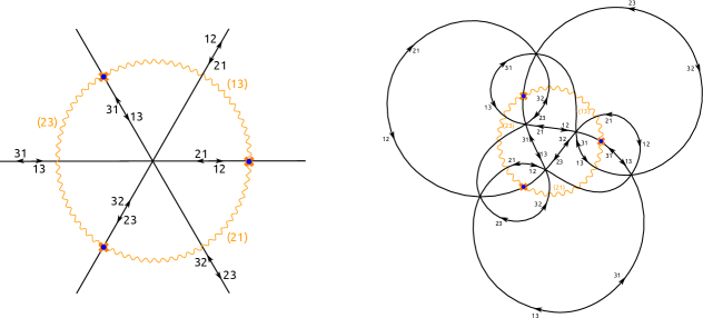
Figure 12: Left: the spectral network $\mathcal{W}(\vartheta_{[1,2]})$. Right: the spectral network $\mathcal{W}(\vartheta_{[1,3]})$. In these figures, for convenience we have chosen the branch cuts differently than in Figure 3.4; the sheet labelings agree inside the unit circle, but differ outside.

As $p$ and $q$ increase, with $p$ and $q$ coprime, the networks $\mathcal{W}(\vartheta_{[p,q]})$ become more intricate. $\mathcal{W}(\vartheta_{[2,5]})$ is shown in Figure 6.3 below.

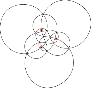
Figure 13: The spectral network $\mathcal{W}(\vartheta_{[2,5]})$. All walls here are double walls, supporting solitons of types $ij$ and $ji$ simultaneously, but we do not show the labels explicitly.

6.4 Joints

One new feature of the networks $\mathcal{W}(\vartheta_{[p,q]})$ is that to compute the soliton counts the constraints (4.19) associated to the punctures are no longer sufficient; we also have to use additional local constraints associated to the joints where six walls meet. These constraints were described in [9] Appendix A. We briefly review them here.

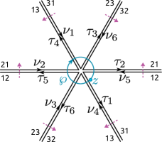
Figure 14: The local picture around a joint.

Up to orientation-preserving diffeomorphisms in the plane, the most general joint which can occur is shown in Figure 6.4.

As in §4.4, we have labeled the walls by symbols $\tau_{n}$ and $\nu_{n}$ for $1\leq n\leq 6$, which we also use to represent the soliton generating functions $\mathbf{S}_{z}$ on the walls. We have also marked a loop $\wp$ on $C$ beginning and ending at the marked point $z$. We write $\wp=\wp_{6}\wp_{5}\cdots\wp_{1}$, where the $\wp_{k}$ are the segments of $\wp$ running between double walls. According to the constraints of §4.3, we have

$$\mathbf{F}_{\wp}=\mathbf{F}_{\wp_{6}}(1-\nu_{5})(1-\tau_{2})\mathbf{F}_{\wp_{5}}(1+\nu_{6})(1+\tau_{3})\mathbf{F}_{\wp_{4}}(1-\nu_{1})(1-\tau_{4})\times\\ \times\mathbf{F}_{\wp_{3}}(1+\nu_{2})(1+\tau_{5})\mathbf{F}_{\wp_{2}}(1-\nu_{3})(1-\tau_{6})\mathbf{F}_{\wp_{1}}(1+\nu_{4})(1+\tau_{1}).$$ (6.8)

Here the $\tau$’s and $\nu$’s are evaluated at the places where $\wp$ crosses the walls, and $\mathbf{F}_{\wp_{k}}$ is the sum of three terms for the lifts of $\wp_{k}$ to $\Sigma$.

Now we can proceed similarly to §4.4: express $\mathbf{F}_{\wp}$ of (6.8) as a matrix, which by homotopy invariance must be equal to the identity matrix; this allows us to determine the “outgoing” $\tau_{n}$ in terms of the “incoming” $\nu_{n}$. For instance,

$$\tau_{1}=\frac{\nu_{1}+\nu_{2}\nu_{6}+\nu_{1}\nu_{3}\nu_{6}+\nu_{1}\nu_{4}\nu_{2}\nu_{6}+\nu_{1}\nu_{3}\nu_{5}\nu_{2}\nu_{6}+\nu_{1}\nu_{3}\nu_{6}\nu_{4}\nu_{2}\nu_{6}}{1-\nu_{1}\nu_{3}\nu_{5}\nu_{4}\nu_{2}\nu_{6}},$$ (6.9)

where the denominator is to be expanded in a geometric series; this gives a series expansion with only positive signs. (Note that this would not have been true if we had chosen different coorientations for the walls in Figure 6.4.)

The expressions for all other $\tau_{n}$ are similar.

6.5 Multiplicities

We can now in principle compute all the BPS counts ${\mathbf{\Omega}}(n\gamma_{[p,q]})$ following the same algorithm described in §5. Unfortunately the computations required for $\mathcal{W}(\vartheta_{[p,q]})$ are generally much more expensive than those for $\mathcal{W}(\vartheta_{[1,0]})$, so we cannot compute as many BPS degeneracies. We just describe here the results for the two networks pictured in Figure 6.3.

For the network $\mathcal{W}(\vartheta_{[1,2]})$, we find:

$n$	${\mathbf{\Omega}}_{\mathrm{red}}(n\gamma_{[1,2]})$
$1$	$\mathbf{78}+3\times\mathbf{1}$
$2$	${\mathbf{650}}+2\times\mathbf{78}+4\times\mathbf{1}$
$3$	${\mathbf{\overline{5824}}}+{\mathbf{5824}}+2\times\mathbf{2925}+8\times\mathbf{650}+11\times\mathbf{78}+12\times\mathbf{1}$

For the network $\mathcal{W}(\vartheta_{[1,3]})$, we have only computed one count with the flavor information included:

$n$	${\mathbf{\Omega}}_{\mathrm{red}}(n\gamma_{[1,3]})$
$1$	$\overline{\mathbf{351}}+3\times\overline{\mathbf{27}}$

Note that the representations of $E_{6}$ which appear here and in §5.4 are constrained: indeed, on a state with charge $\gamma_{[p,q]}$, the generator $\mathcal{C}$ of the $\mathbb{Z}_{3}$ center (see Appendix A for our conventions) acts by $\omega^{p+q}$. So, at least as far as the BPS states of theory $T_{3}$ are concerned, it appears that there is a slight mixing between the electromagnetic symmetry and the flavor symmetry. It would be nice to understand this on some a priori ground.

The flavorless BPS degeneracies for both of these networks can be easily computed up to $n=13$. The results are

$n$	$\Omega_{\mathrm{red}}(n\gamma_{[1,2]})$
$1$	$81$
$2$	$810$
$3$	$23568$
$4$	$1054620$
$5$	$59272560$
$6$	$3845869602$
$7$	$275518046160$
$8$	$21220796005632$
$9$	$1727362288212480$
$10$	$146871096341656590$
$11$	$12936006724475199888$
$12$	$1173014876208454094700$
$13$	$108997909913288073225456$

and

$n$	$\Omega_{\mathrm{red}}(n\gamma_{[1,3]})$
$1$	$432$
$2$	$63126$
$3$	$25837040$
$4$	$15997511988$
$5$	$12414634813584$
$6$	$11112471629495966$
$7$	$10976477695048905264$
$8$	$11652623904520407820032$
$9$	$13070660396858566472984064$
$10$	$15312115043824353889100152626$
$11$	$18579553424056358193512622811248$
$12$	$23208045406405864226170364128108836$
$13$	$29704725146725768042434236249559752976$

7 A picture of the lightest states

For the lightest BPS states counted by a given spectral network, the recipe which we reviewed in §5.2 simplifies considerably. Indeed, let $\gamma$ be the charge of these states; then for each double wall $p$, to compute the coefficient ${\boldsymbol{\alpha}}_{1}(p)$ we only need to study the lightest solitons supported on $p$:

$${\boldsymbol{\alpha}}_{1}(p)=\tau_{{\mathrm{li}}}(p)\nu_{{\mathrm{li}}}(p),$$ (7.1)

where $\tau_{{\mathrm{li}}},\nu_{{\mathrm{li}}}$ are the truncations of $\tau,\nu$ to the lightest soliton charges — i.e. we keep only the first term in the expansion in powers of $X_{\gamma}$. Then we use the rule (5.19) which says

$${\mathbf{L}}(\gamma)=\sum_{p}{\boldsymbol{\alpha}}_{1}(p)p_{\Sigma},$$ (7.2)

and as above

$${\mathbf{\Omega}}(\gamma)={\mathbf{L}}(\gamma)/[\gamma].$$ (7.3)

The lightest solitons are relatively easy to compute with bare hands, and lead to simple geometric pictures of what the BPS index ${\mathbf{\Omega}}(\gamma)$ is counting. Informally speaking, we just have to count the possible ways of “gluing together two solitons head-to-head.” We now illustrate this in a few examples.

7.1 Lightest states with charge $\gamma_{1}=\gamma_{[1,0]}$

In this section we reconsider the result ${\mathbf{\Omega}}(\gamma_{1})=\mathbf{\overline{27}}$, which we obtained in (5.24).

We consider the truncated spectral networks $\mathcal{W}(\vartheta_{1})[\Lambda]$. Let us start with $\Lambda\ll M$. As shown in Figure 4.5 above, each puncture $z_{\ell}$ emits three light solitons in opposite directions, carrying the flavor representations $\mathbf{3}_{\ell}$ and $\mathbf{\overline{3}}_{\ell}$. The resulting network is shown on the left in Figure 7.1.

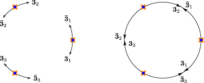
Figure 15: Solitons in the truncated network $\mathcal{W}(\vartheta_{1})[\Lambda]$ for increasing values of $\Lambda$. Left: the network at $\Lambda=0.25M$. The wall with label $\mathbf{3}_{1}$ represents three light solitons in the fundamental representation of $SU(3)_{1}$, etc. Right: the truncated network at $\Lambda=M$. Here the walls have grown just far enough to reach the adjacent punctures.

As we increase $\Lambda$, the walls of the network extend, until at $\Lambda=M$ they reach the neighboring punctures. The resulting network and soliton data are shown on the right in Figure 7.1. From this figure we obtain

$${\boldsymbol{\alpha}}_{1}(p_{1})=({\bf\overline{3}},{\bf 3},{\bf 1}),\quad{\boldsymbol{\alpha}}_{1}(p_{2})=({\bf 1},{\bf\overline{3}},{\bf 3}),\quad{\boldsymbol{\alpha}}_{1}(p_{3})=({\bf 3},{\bf 1},{\bf\overline{3}}).$$ (7.4)

Then, according to (7.2), ${\mathbf{L}}(\gamma_{1})$ is a sum over the three wall segments:

$${\mathbf{L}}(\gamma_{1})=({\bf\overline{3}},{\bf 3},{\bf 1})\gamma+({\bf 1},{\bf\overline{3}},{\bf 3})\gamma+({\bf 3},{\bf 1},{\bf\overline{3}})\gamma,$$ (7.5)

from which we read off using (7.3)

$${\mathbf{\Omega}}(\gamma_{1})=(\bf\overline{3},\bf 3,\bf 1)+(\bf 1,\bf\overline{3},\bf 3)+(\bf 3,\bf 1,\bf\overline{3}),$$ (7.6)

i.e. ${\mathbf{\Omega}}(\gamma_{1})=\bf{\overline{27}}$, recovering (5.24) as desired.

7.2 Lightest states with charge $\gamma_{[1,2]}$

Next, we reconsider the BPS states of charge $\gamma_{[1,2]}$. Figure 7.2 and 7.2 show a few of the relevant spectral networks at increasing values of $0<\Lambda\leq M_{\gamma_{[1,2]}}$.

As above, for small $\Lambda$ each puncture emits 3 walls in each direction. These walls are shown on the left in Figure 7.2. At $\Lambda=\frac{1}{3}M_{\gamma_{[1,2]}}$ these walls meet each other at the two joints at $z=0,\infty$.

Let us study what happens at the joint at $z=0$. If we substitute $\nu_{12}=\nu_{23}=\nu_{31}=0$ into the soliton rules obtained by solving (6.8), we find

$$\tau_{21}=\nu_{21}, \tau_{32}=\nu_{32}, \tau_{13}=\nu_{13},$$ (7.7)

$$\tau_{12}=\nu_{13}\nu_{32}, \tau_{23}=\nu_{21}\nu_{13}, \tau_{31}=\nu_{32}\nu_{21}.$$ (7.8)

The first line (7.7) implies that the original walls continue to extend beyond the joint, with the same soliton degeneracies as before. The second line says that, in addition, there are new walls born at the joint, whose soliton degeneracies are the product of the incoming ones; so the new walls support solitons with flavor charge $\mathbf{3}\times\mathbf{3}$. Their mass at the joint is $\frac{2}{3}M_{\gamma_{[1,2]}}$, the sum of the two constituent masses. These new walls thus only show up when $\Lambda\geq\frac{2}{3}M_{\gamma_{[1,2]}}$.

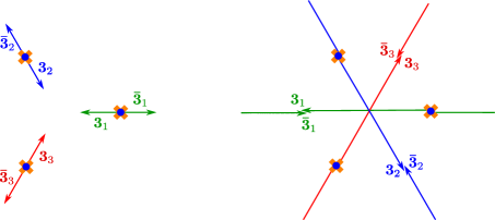
Figure 16: Left: the truncated network $\mathcal{W}(\vartheta_{[1,2]})[\Lambda]$ at $\Lambda=\frac{1}{6}M_{\gamma_{[1,2]}}$. The walls with label $\mathbf{3}$ and $\mathbf{\overline{3}}$ represent the lightest solitons emerging from the punctures. Right: the truncation at $\Lambda=\frac{1}{2}M_{\gamma_{[1,2]}}$.

The right of Figure 7.2 shows the truncation at $\Lambda=\frac{1}{2}M_{\gamma_{[1,2]}}$. At this moment the original walls have extended past the joints, but the new walls have not yet been born. The left of Figure 7.2 shows the truncation at $\Lambda=\frac{2}{3}M_{\gamma_{[1,2]}}$, when the new walls with label $\mathbf{3}\times\mathbf{3}$ appear in the network, emanating from the joint $z=0$. Simultaneously, the original walls with label $\overline{\mathbf{3}}$ reach the joint. Thus the new wall born from the joint at $z=0$ carries solitons transforming in $\overline{\mathbf{3}}+\mathbf{3}\times\mathbf{3}$. Similar comments apply to $z=\infty$. Finally, at $\Lambda=M_{\gamma_{[1,2]}}$ all walls arrive at punctures. This is illustrated on the right of Figure 7.2.

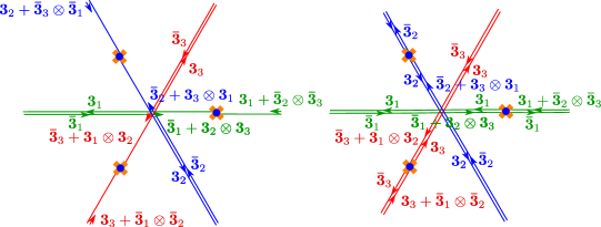
Figure 17: Left: the truncation at $\Lambda=\frac{2}{3}M_{\gamma_{[1,2]}}$. The initial walls reach the second joint and simultaneously the new walls in the tensor product representation appear. Together they combine into walls with label $\mathbf{3}+\mathbf{\overline{3}}\otimes\mathbf{\overline{3}}$. Right: the truncation at $\Lambda=M_{\gamma_{[1,2]}}$.

Let ${p}_{\ell}^{a}$ be the wall segment running between the joint at $z=0$ and the puncture $z_{\ell}$, let ${p}_{\ell}^{b}$ be the wall segment between the puncture $z_{\ell}$ and the joint at $z=\infty$, and let $p_{\ell}^{c}$ be the wall segment running between $z=\infty$ and $z=0$. Then we read off from Figure 7.2

$${\boldsymbol{\alpha}}_{1}(p_{\ell}^{a})={\bf{3}}_{\ell}\otimes({\bf{\overline{3}}}_{\ell}\oplus{\bf{3}}_{\ell^{\prime}}\otimes{\bf{3}}_{\ell^{\prime\prime}}),\quad{\boldsymbol{\alpha}}_{1}(p_{\ell}^{b})={\bf{\overline{3}}}_{\ell}\otimes({\bf{3}}_{\ell}\oplus{\bf{\overline{3}}}_{\ell^{\prime}}\otimes{\bf{\overline{3}}}_{\ell^{\prime\prime}}),\quad{\boldsymbol{\alpha}}_{1}(p_{\ell}^{c})={\bf{3}}_{\ell}\otimes{\bf{\overline{3}}}_{\ell},$$ (7.9)

where we defined $\ell^{\prime}=\ell+1$, $\ell^{\prime\prime}=\ell+2$.

Now we use (7.2) to determine ${\mathbf{L}}(\gamma)$. A new feature appearing in this case is that the individual lifts $p_{\Sigma}$ are not closed cycles: rather, we only get closed cycles once we sum up. Nevertheless we can organize the answer into a sum over $5$ finite string webs, as follows. We define formal sums

$$w^{1}_{\ell}=p^{a}_{\ell}+p^{b}_{\ell}+p^{c}_{\ell},\quad w^{2}=\sum_{\ell=1}^{3}{p}^{a}_{\ell},\quad w^{3}=\sum_{\ell=1}^{3}p^{b}_{\ell}.$$ (7.10)

The webs $w^{1}_{\ell}$ and $w^{2}$ are illustrated in Figure 7.2.

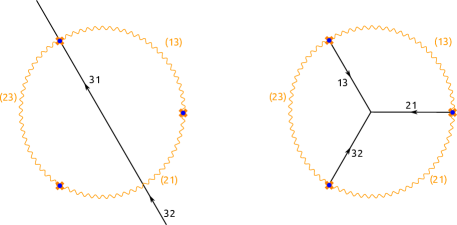
Figure 18: BPS string webs of charge $\gamma_{[1,2]}$. Left: string web $w^{1}_{2}$ with coefficient $(\bf 1,\bf{3}\otimes\bf\overline{3},\bf 1)$. Right: string web $w^{2}$ with coefficient $(\bf 3,\bf 3,\bf 3)$.

Even though each of the finite webs $w^{1}_{\ell}$, $w^{2}$ and $w^{3}$ has a different topology, lifting each web to $\Sigma$ yields a 1-cycle in the single homology class $\gamma_{[1,2]}$. The lifts of the string webs $w^{1,2}$ and $w^{2}$ are shown in Figure 7.2.

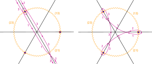
Figure 19: Lifts of the string webs in Figure 7.2 to $\Sigma$.

The cycle ${\mathbf{L}}(\gamma)$ given by (7.2) decomposes nicely in terms of the lifts of these $5$ webs:

$${\mathbf{L}}(\gamma)=\sum_{\ell=1}^{3}({\bf 3}_{\ell}\otimes{\overline{\bf 3}}_{\ell})(w^{1}_{\ell})_{\Sigma}+({\bf 3},{\bf 3},{\bf 3})w^{2}_{\Sigma}+({\bf\overline{3}},{\bf\overline{3}},{\bf\overline{3}})w^{3}_{\Sigma}.$$ (7.11)

We therefore find

$${\mathbf{\Omega}}(\gamma_{[1,2]}) =(\bf{3}\otimes\bf\overline{3},\bf 1,\bf 1)+(\bf 1,\bf{3}\otimes\bf\overline{3},\bf 1)+(1,1,\bf{3}\otimes\bf\overline{3})+(\bf 3,\bf 3,\bf 3)+(\bf\overline{3},\bf\overline{3},\bf\overline{3})$$ (7.12)

$$=({\bf 3},{\bf 3},{\bf 3})+({\bf\overline{3}},{\bf\overline{3}},{\bf\overline{3}})+({\bf{8}},{\bf 1},{\bf 1})+({\bf 1},{\bf{8}},{\bf 1})+({\bf 1},{\bf 1},{\bf{8}})+3\times({\bf 1},{\bf 1},{\bf 1}),$$ (7.13)

where each of the terms in the first line is directly associated to one of the five string webs. This is the decomposition of the representation $\mathbf{78}+3\times\mathbf{1}$ of $E_{6}$, matching the result we reported in §6.5.

7.3 Lightest states with charge $\gamma_{[1,3]}$

Finally we revisit the states of charge $\gamma_{[1,3]}$. Figures 7.3-7.3 illustrate the truncated networks relevant for the computation of ${\mathbf{\Omega}}(\gamma_{[1,3]})$.

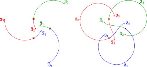
Figure 20: Left: the truncated network $\mathcal{W}(\vartheta_{[1,3]})[\Lambda]$ at $\Lambda=0.2M_{\gamma_{[1,3]}}$. At $\Lambda=\frac{2}{7}M_{\gamma_{[1,3]}}$ some of the walls meet. Right: the truncation at $\Lambda=0.32M_{\gamma_{[1,3]}}$.

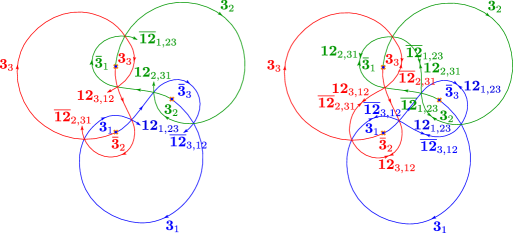
Figure 21: At $\Lambda=\frac{3}{7}M_{\gamma_{[1,3]}}$, new walls with label $\mathbf{\overline{3}}\otimes\mathbf{\overline{3}}$ are born from $3$ of the joints. At the same moment, walls with label $\mathbf{3}$ arrive at these joints. Thus the walls emerging from the joints carry the composite label $\mathbf{12}=\mathbf{3}+\mathbf{\overline{3}}\otimes\mathbf{\overline{3}}$. At the other $3$ joints we get similar walls with the complex conjugate labels. Left: the truncation at $\Lambda=0.44M_{\gamma_{[1,3]}}$. At $\Lambda=\frac{4}{7}M_{\gamma_{[1,3]}}$ the walls with labels $\mathbf{12}$ and $\mathbf{\overline{12}}$ arrive at the next joint. At this joint, solitons are generated which have $M=\frac{8}{7}M_{\gamma_{[1,3]}}$ and thus do not contribute to the spectrum of states with mass $M_{\gamma_{[1,3]}}$. Right: the truncation at $\Lambda=0.64M_{\gamma_{[1,3]}}$.

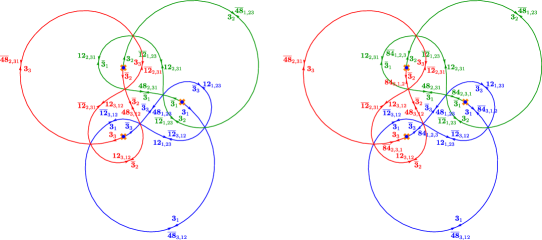
Figure 22: At $\Lambda=\frac{5}{7}M_{\gamma_{[1,3]}}$ the walls with label $\mathbf{12}$ arrive at the next joint. This generates new solitons in the representation $\mathbf{48}=\mathbf{12}+\mathbf{\overline{3}}\otimes\mathbf{\overline{12}}$. Left: the truncation at $\Lambda=0.78M_{\gamma_{[1,3]}}$. At $\Lambda=\frac{6}{7}M_{\gamma_{[1,3]}}$ the new walls cross the final joint. This generates solitons in the representation $\mathbf{84}=\mathbf{48}+\mathbf{\overline{3}}\otimes\mathbf{\overline{12}}$ (and complex conjugate). Right: the truncation at $\Lambda=M_{\gamma_{[1,3]}}.$

In the final truncation at the right in Figure 7.3, each colored wall consists of 7 segments. For the wall colored red, the values of ${\boldsymbol{\alpha}}_{1}$ on these 7 segments are

$${\bf{\overline{3}}}_{2}\otimes{\bf{84}}_{3,1,2},\ {\bf{\overline{3}}}_{2}\otimes{\bf{48}}_{3,12},\ {\bf{\overline{3}}}_{2}\otimes{\bf{12}}_{3,12},\ {\bf{\overline{12}}}_{2,31}\otimes{\bf{12}}_{3,12},\ {\bf{\overline{12}}}_{2,31}\otimes{\bf{3}}_{3},\ {\bf{\overline{48}}}_{2,31}\otimes{\bf{3}}_{3},\ {\bf{\overline{84}}}_{2,3,1}\otimes{\bf{3}}_{3},$$ (7.14)

where we defined convenient combinations of representations:

$$\mathbf{12}_{3,12} =\mathbf{3}_{3}+\mathbf{\overline{3}}_{1}\otimes\mathbf{\overline{3}}_{2},$$ (7.15)

$$\mathbf{48}_{3,12} =\mathbf{12}_{3,12}+\mathbf{\overline{3}}_{3}\otimes\mathbf{\overline{12}}_{3,12},$$ (7.16)

$$\mathbf{84}_{2,3,1} =\mathbf{48}_{2,31}+\mathbf{\overline{3}}_{2}\otimes\mathbf{\overline{12}}_{1,23}.$$ (7.17)

For the other two walls (blue and green), the values of ${\boldsymbol{\alpha}}_{1}$ are obtained from (7.14) by a cyclic permutation of the indices $123$.

As in the last example, we can realize the resulting ${\mathbf{L}}(\gamma)$ as a sum over string webs $w$. There are $12$ such webs, some of which are illustrated in Figure 7.3 and Figure 7.3. (The ones that are not shown can be obtained by applying rotations by multiples of $\frac{2\pi}{3}$ to the ones shown.)

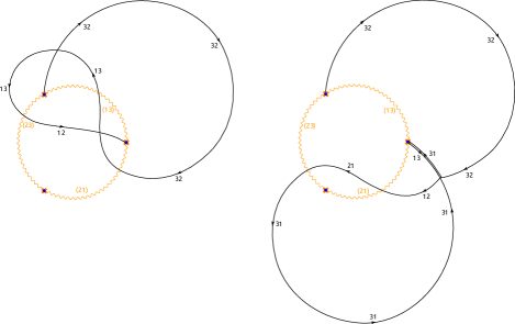
Figure 23: BPS string webs of charge $\gamma_{[1,3]}$. Left: string web with coefficient $(\mathbf{\overline{3}},\mathbf{3},\mathbf{1})$. Right: string web with coefficient $(\mathbf{3\otimes 3},\mathbf{3},\mathbf{1})$.

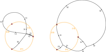
Figure 24: More BPS string webs of charge $\gamma_{[1,3]}$. Left: string web with coefficient $(\mathbf{\overline{3}\otimes\overline{3}},\mathbf{1},\mathbf{\overline{3}})$. Right: string web with coefficient $(\mathbf{3},\mathbf{3\otimes\overline{3}},\mathbf{\overline{3}})$.

All these webs lift to 1-cycles on $\Sigma$ in the same homology class $\gamma_{[1,3]}$. We therefore find

$${\mathbf{\Omega}}(\gamma_{[1,3]})=~{} ({\bf 3}\otimes{\bf\overline{3}},{\bf\overline{3}},{\bf{3}})+({\bf{3}},{\bf 3}\otimes{\bf\overline{3}},{\bf\overline{3}})+({\bf\overline{3}},{\bf{3}},{\bf 3}\otimes{\bf\overline{3}})+({\bf 1},{\bf\overline{3}},{\bf\overline{3}}\otimes{\bf\overline{3}})$$ (7.18)

$$+({\bf\overline{3}}\otimes{\bf\overline{3}},{\bf 1},{\bf\overline{3}})+({\bf\overline{3}},{\bf\overline{3}}\otimes{\bf\overline{3}},{\bf 1})+({\bf{3}}\otimes{\bf{3}},{\bf{3}},{\bf 1})+({\bf{3}},{\bf 1},{\bf{3}}\otimes{\bf{3}})$$

$$+({\bf 1},{\bf{3}}\otimes{\bf{3}},{\bf{3}})+({\bf{3}},{\bf 1},{\bf\overline{3}})+({\bf 1},{\bf\overline{3}},{\bf{3}})+({\bf\overline{3}},{\bf{3}},{\bf 1})$$

$$=~{} ({\bf 8},{\bf\overline{3}},{\bf 3})+({\bf 3},{\bf 8},{\bf\overline{3}})+({\bf\overline{3}},{\bf 3},{\bf 8})+({\bf 1},{\bf\overline{3}},{\bf\overline{6}})+({\bf\overline{6}},{\bf 1},{\bf\overline{3}})+({\bf\overline{3}},{\bf\overline{6}},{\bf 1})$$ (7.19)

$$+({\bf 6},{\bf 3},{\bf 1})+({\bf 3},{\bf 1},{\bf 6})+({\bf 1},{\bf 6},{\bf 3})+4\times({\bf 3},{\bf 1},{\bf\overline{3}})+4\times({\bf 1},{\bf\overline{3}},{\bf 3})+4\times({\bf\overline{3}},{\bf 3},{\bf 1}),$$

where each of the terms in (7.18) has an interpretation as a flavor multiplet of BPS states associated to one of the $12$ webs. The result (7.19) is the decomposition of the representation $\mathbf{\overline{351}}+3\times\mathbf{\overline{27}}$ of $E_{6}$, matching what we stated in §6.5.

7.4 Arbitrary $(p,q)$

Finally we can discuss more general $\gamma_{[p,q]}$. We will show that $\Omega(\gamma_{[p,q]})>0$ for any $p,q$ with $(p,q)=1$, i.e., BPS states exist with all primitive electromagnetic charges.

For this purpose we need some general way of understanding what the networks $\mathcal{W}(\vartheta_{[p,q]})$ look like. This turns out to be surprisingly easy: as we now explain, we can relate the walls of $\mathcal{W}(\vartheta_{[p,q]})$ to straight-line trajectories on an auxiliary torus. (This is similar to a construction used in [8] Section 10.7 to analyze the spectrum of ${\mathcal{N}}=2$ supersymmetric $SU(2)$ Yang-Mills with $4$ hypermultiplet flavors.)

If we choose a soliton central charge $Z_{a}$ for $a\in\Gamma_{ij,zz}$ as a local coordinate around $z$, then in this coordinate the walls of $\mathcal{W}(\vartheta)$ carrying label $ij$ are just straight lines of inclination $\vartheta$ (this follows immediately from the definition of $\mathcal{W}(\vartheta)$.) Shifting $a$ to $a+\gamma$ has the effect of shifting the coordinate $Z_{a}$ by $Z_{\gamma}$, which by (2.7) lies in the lattice

$$\Xi=(\mathbb{Z}\oplus\omega\mathbb{Z})M.$$ (7.20)

We also have the $\mathbb{Z}_{3}$ action $\rho:\Gamma_{ij,zz}\to\Gamma_{i+1,j+1,zz}$, which has $Z_{\rho(a)}=\omega Z_{a}$. Thus, if $a\in\Gamma_{ij,zz}$ and $a^{\prime}\in\Gamma_{kl,zz}$, $Z_{a}$ and $Z_{a^{\prime}}$ differ by the composition of translation by an element of $\Xi$ and multiplication by some power of $\omega$. Said otherwise, mapping a point $z\in C$ to the collection of all soliton central charges $Z_{a}$ at $z$ gives a map

$$\phi:C\to T^{2}/\mathbb{Z}_{3},\qquad T^{2}=\mathbb{C}/\Xi.$$ (7.21)

This map takes all three punctures of $C$ to the point $0\in T^{2}$. Lifting $\phi(\mathcal{W}(\vartheta))$ from $T^{2}/\mathbb{Z}_{3}$ to $T^{2}$ (just taking the inverse image), we obtain a collection of straight lines on $T^{2}$, with inclinations $\vartheta+\frac{2n\pi}{3}$. This collection must contain at least the $3$ straight lines emanating from $0\in T^{2}$. In Figure 7.4 we show these lines for $\vartheta=\vartheta_{[p,q]}$ with $(p,q)=(1,0)$, $(1,2)$, and $(1,3)$.

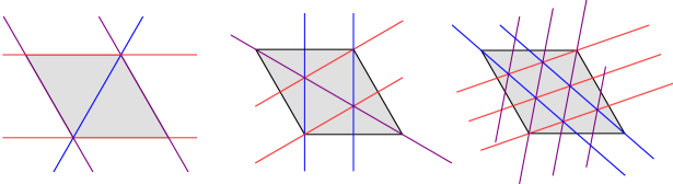
Figure 25: The walls of $\mathcal{W}(\vartheta_{[p,q]})$ lifted to a fundamental domain of $T^{2}=\mathbb{C}/\Xi$, for $(p,q)=(1,0)$, $(1,2)$, and $(1,3)$.

If there are any other walls of $\mathcal{W}(\vartheta)$, they must emanate from intersections between the walls we have already drawn. Now, any intersection between the walls on $C$ would lead to an intersection between our lifted lines on $T^{2}$. Looking at Figure 7.4, we see that for $\vartheta=\vartheta_{[p,q]}$ some such intersections do exist, but we will not obtain any new lines on $T^{2}$ in this way: all six possible directions in which a new line could emanate are already populated. We also see that, when $\vartheta=\vartheta_{[p,q]}$, the lifted walls are all closed loops on $T^{2}$. (In contrast, for all other phases $\vartheta$, the lifted walls run around $T^{2}$ forever, filling it up densely.)

Each joint on $C$ maps to an intersection on $T^{2}/\mathbb{Z}_{3}$, thus to $3$ intersections on the covering $T^{2}$. On the other hand, there is also a $\mathbb{Z}_{3}$ action on $C$ by $z\mapsto\omega z$, under which $\phi$ is invariant; joints related by this symmetry map to the same intersection on $T^{2}/\mathbb{Z}_{3}$. There is an exceptional case if a joint occurs at $z=0$ or $z=\infty$: then it is a fixed point of the $\mathbb{Z}_{3}$ action on $C$, and also its image is a fixed point of the $\mathbb{Z}_{3}$ action on $T^{2}$. Thus, in all cases the number of intersections on $T^{2}$ (excluding the point $0$) is the same as the number of six-way joints between walls in $\mathcal{W}(\vartheta)$. Comparing Figure 7.4 with Figures 3.4, 6.3 we see that the numbers $0$, $2$, $6$ of intersections indeed match the corresponding numbers of joints. However, we stress that there is not a natural 1:1 correspondence between the joints and the intersections, nor between the walls on $C$ and the lines on $T^{2}$.

Nevertheless, we can read out from this picture useful facts about the walls on $C$:

• Each wall, when continued far enough in either direction, ends on a puncture.

• The “lengths” of all wall segments on $C$ — as measured by the change in the soliton mass as we move along the wall — are equal. (This follows from the fact that the segments on $T^{2}$ have equal length, as visible in Figure 7.4.)

• There exists a global coorientation of all walls on $C$, such that the local picture around each joint matches Figure 6.4. (This coorientation corresponds to one of the two possible $\mathbb{Z}_{3}$-invariant coorientations of the lines on $T^{2}$.)

• With this coorientation, the local picture around each puncture matches Figure 4.4. (To see this, first note an invariant characterization of the coorientation in Figure 4.4: the outgoing wall of type $i,i+1$ has coorientation corresponding to going clockwise around the puncture, and the outgoing wall of type $i+1,i$ has coorientation going counterclockwise. On the other hand, in Figure 6.4, the incoming walls of type $i,i+1$ have the counterclockwise coorientation around the joint, and the incoming walls of type $i+1,i$ have the clockwise coorientation. These two are compatible, as desired.)

The existence of this global coorientation, together with the fact that all signs in the expansion of (6.9) and (4.19) are positive, shows that the soliton generating functions $\tau$, $\nu$ have all coefficients nonnegative. In particular, this is true of $\tau_{\mathrm{li}}$ and $\nu_{\mathrm{li}}$. It follows that (letting $\gamma=\gamma_{[p,q]}$)

$$L(\gamma)=\sum_{p}c_{p}p_{\Sigma}$$ (7.22)

where all $c_{p}>0$, and the sum runs over all double walls (moreover, since all walls end on punctures, this sum is nonempty.) Now, we can restate (5.9) as

$$\Omega(\gamma)=\frac{\int_{L(\gamma)}{\mathrm{e}}^{-{\mathrm{i}}\vartheta}\lambda}{\int_{\gamma}{\mathrm{e}}^{-{\mathrm{i}}\vartheta}\lambda}=\sum_{p}c_{p}\frac{\int_{p_{\Sigma}}{\mathrm{e}}^{-{\mathrm{i}}\vartheta}\lambda}{\int_{\gamma}{\mathrm{e}}^{-{\mathrm{i}}\vartheta}\lambda}$$ (7.23)

and recalling that both $\int_{p_{\Sigma}}{\mathrm{e}}^{-{\mathrm{i}}\vartheta}\lambda$ and $\int_{\gamma}{\mathrm{e}}^{-{\mathrm{i}}\vartheta}\lambda$ are negative real numbers, we conclude that

$$\Omega(\gamma)>0$$ (7.24)

as we claimed.

Appendix A $E_{6}$ representations

We label the nodes of the $E_{6}$ Dynkin diagram by:

Then our names for the representations are:

Dynkin labels	Representation
000000	$\mathbf{1}$
100000	$\mathbf{27}$
000010	$\overline{\mathbf{27}}$
000001	$\mathbf{78}$
010000	$\overline{\mathbf{351}}$
000100	$\mathbf{351}$
200000	$\overline{\mathbf{351}}^{\prime}$
100010	$\mathbf{650}$
100001	$\mathbf{1728}$
000011	$\overline{\mathbf{1728}}$
000002	$\mathbf{2430}$
001000	$\mathbf{2925}$
110000	$\mathbf{5824}$
100100	$\overline{\mathbf{7371}}$
010001	$\overline{\mathbf{17550}}$
200001	$\overline{\mathbf{19305}}$

These are the names used in the Mathematica package LieART [33], which we used to perform computations.

We let $\mathcal{C}$ denote a generator of the center $\mathbb{Z}_{3}$ of the compact simply connected form of $E_{6}$. On a representation with Dynkin labels $(a_{1},\dots,a_{6})$, $\mathcal{C}$ acts by the cube root of unity

$$\omega^{a_{1}-a_{2}+a_{4}-a_{5}}.$$ (A.1)

So e.g. $\mathcal{C}$ acts as $\omega$ on the representations ${\mathbf{27}}$ and ${\mathbf{1728}}$, as $\omega^{-1}$ on $\overline{\mathbf{27}}$, and trivially on the adjoint ${\mathbf{78}}$.

Our conventions for the $SU(3)\times SU(3)\times SU(3)/\mathbb{Z}_{3}$ subgroup of $E_{6}$ are fixed by specifying the decomposition of the representation ${\mathbf{27}}$:

$${\mathbf{27}}=(\mathbf{3},\mathbf{\overline{3}},\mathbf{1})+(\mathbf{1},\mathbf{3},\mathbf{\overline{3}})+(\mathbf{\overline{3}},\mathbf{1},\mathbf{3}).$$ (A.2)

(This does not match the conventions of LieART: to compare, one needs to act by the nontrivial outer automorphism of the first $SU(3)$ factor, which has the effect of conjugating the representations of that factor.)

References

- [1] J. A. Minahan and D. Nemeschansky, “An N = 2 superconformal fixed point with E(6) global symmetry,” Nucl. Phys. B482 (1996) 142–152, hep-th/9608047.
- [2] N. Seiberg, “Five-dimensional SUSY field theories, nontrivial fixed points and string dynamics,” Phys. Lett. B388 (1996) 753–760, hep-th/9608111.
- [3] J. A. Minahan and D. Nemeschansky, “Superconformal fixed points with E(n) global symmetry,” Nucl. Phys. B489 (1997) 24–46, hep-th/9610076.
- [4] O. Aharony and Y. Tachikawa, “A Holographic computation of the central charges of d=4, N=2 SCFTs,” JHEP 01 (2008) 037, 0711.4532.
- [5] A. Gadde, L. Rastelli, S. S. Razamat, and W. Yan, “The Superconformal Index of the SCFT,” JHEP 08 (2010) 107, 1003.4244.
- [6] A. Gadde, S. S. Razamat, and B. Willett, ““Lagrangian” for a Non-Lagrangian Field Theory with Supersymmetry,” Phys. Rev. Lett. 115 (2015), no. 17, 171604, 1505.05834.
- [7] D. Gaiotto, “N=2 dualities,” 0904.2715.
- [8] D. Gaiotto, G. W. Moore, and A. Neitzke, “Wall-crossing, Hitchin systems, and the WKB approximation,” Adv. Math. 234 (2013) 239–403, 0907.3987.
- [9] D. Gaiotto, G. W. Moore, and A. Neitzke, “Spectral networks,” Annales Henri Poincaré 14 (November, 2013) 1643–1731, 1204.4824.
- [10] D. Galakhov, P. Longhi, and G. W. Moore, “Spectral networks with spin,” 1408.0207.
- [11] C. Cordova and T. Dumitrescu, “Current algebra constraints on BPS particles.” To appear.
- [12] M. Huang, A. Klemm, and M. Poretschkin, “Refined stable pair invariants for -, - and -strings,” 1308.0619.
- [13] M. Alim, S. Cecotti, C. Cordova, S. Espahbodi, A. Rastogi, and C. Vafa, “ quantum field theories and their BPS quivers,” Adv. Theor. Math. Phys. 18 (2014), no. 1, 27–127, 1112.3984.
- [14] D. Gaiotto, G. W. Moore, and A. Neitzke, “Spectral Networks and Snakes,” 1209.0866.
- [15] K. Maruyoshi, C. Y. Park, and W. Yan, “BPS spectrum of Argyres-Douglas theory via spectral network,” 1309.3050.
- [16] M. Gabella, “Quantum Holonomies from Spectral Networks and Framed BPS States,” 1603.05258.
- [17] P. Longhi and C. Y. Park, “ADE Spectral Networks,” 1601.02633.
- [18] A. Neitzke, “swn-plotter.” Available at http://www.ma.utexas.edu/users/neitzke/mathematica/swn-plotter.nb.
- [19] D. Gaiotto, “Surface Operators in N=2 4d Gauge Theories,” 0911.1316.
- [20] D. Gaiotto, G. W. Moore, and A. Neitzke, “Wall-crossing in coupled 2d-4d systems,” JHEP 12 (2012) 1103.2598.
- [21] S. Cecotti, P. Fendley, K. A. Intriligator, and C. Vafa, “A new supersymmetric index,” Nucl. Phys. B386 (1992) 405–452, hep-th/9204102.
- [22] D. Galakhov, P. Longhi, T. Mainiero, G. W. Moore, and A. Neitzke, “Wild Wall Crossing and BPS Giants,” 1305.5454.
- [23] N. Drukker, D. Gaiotto, and J. Gomis, “The Virtue of Defects in 4D Gauge Theories and 2D CFTs,” 1003.1112.
- [24] N. Drukker, D. R. Morrison, and T. Okuda, “Loop operators and S-duality from curves on Riemann surfaces,” 0907.2593.
- [25] D. Gaiotto, G. W. Moore, and A. Neitzke, “Framed BPS States,” Adv. Theor. Math. Phys. 17 (2013), no. 2, 241–397, 1006.0146.
- [26] R. Koberle and V. Kurak, “Solitons in the Supersymmetric Model,” Phys. Rev. D36 (1987) 627.
- [27] E. Getzler and M. M. Kapranov, “Modular operads,” Compositio Math. 110 (1998), no. 1, 65–126.
- [28] B. Feng, A. Hanany, and Y.-H. He, “Counting gauge invariants: The Plethystic program,” JHEP 03 (2007) 090, hep-th/0701063.
- [29] D. Gaiotto, A. Strominger, and X. Yin, “New connections between 4D and 5D black holes,” hep-th/0503217.
- [30] R. Dijkgraaf, C. Vafa, and E. Verlinde, “M-theory and a topological string duality,” hep-th/0602087.
- [31] T. Mainiero, “Algebraicity and Asymptotics: An explosion of BPS indices from algebraic generating series,” 1606.02693.
- [32] C. Cordova and S.-H. Shao, “Asymptotics of ground state degeneracies in quiver quantum mechanics,” 1503.03178.
- [33] R. Feger and T. W. Kephart, “LieART — A Mathematica application for Lie algebras and representation theory,” Comput. Phys. Commun. 192 (2015) 166–195, 1206.6379.