A maximum entropy approach to separating noise from signal in bimodal affiliation networks

Abstract

In practice, many empirical networks, including co-authorship and collocation networks are unimodal projections of a bipartite data structure where one layer represents entities, the second layer consists of a number of sets representing affiliations, attributes, groups, etc., and an interlayer link indicates membership of an entity in a set. The edge weight in the unimodal projection, which we refer to as a co-occurrence network, counts the number of sets to which both end-nodes are linked. Interpreting such dense networks requires statistical analysis that takes into account the bipartite structure of the underlying data. Here we develop a statistical significance metric for such networks based on a maximum entropy null model which preserves both the frequency sequence of the individuals/entities and the size sequence of the sets. Solving the maximum entropy problem is reduced to solving a system of nonlinear equations for which fast algorithms exist, thus eliminating the need for expensive Monte-Carlo sampling techniques. We use this metric to prune and visualize a number of empirical networks.

I Introduction

Many integer weighted graphs derived from empirical data are so-called co-occurrence graphs: an edge weight counts the number of times the two end nodes where observed to share a property. Most abstractly, this shared property can be modeled as membership in some unordered set. For instance, membership in the same team or group, affiliation with an institution, shared physical attributes, or words appearing in the same document. Such networks have been studied in various contexts including co-attendance in social events davis2009DeepSouth , networks of co-starring actors watts1998collective congressional bill co-sponsorship networks fowler2006connecting ; fowler2006legislative .

Formally, given a set $S=\{s_{1},s_{2},\cdots,s_{m}\}$ of symbols or entities, the data consists of an arbitrary number of subsets of $S:$

$$D=\left\{u_{j}\right\}_{j=1}^{n},\,\,\,\,\,u_{j}\subset S\,\,\,\,j=1,\cdots n.$$ (1)

In its simplest form, a given entry $u_{j}$ is simply an unordered set defining a symmetric relationship between every pair of its elements. A weighted graph may then be defined with vertex set $V\equiv S$ where a weighted edge between two nodes counts the number of subsets $u_{j}$ containing both nodes. In the context of natural language processing, the subsets $u_{j}$ are commonly referred to as documents and their elements as words or symbols. The set $S$ is sometimes referred to as the Lexicon. We will use this terminology in the rest of this paper.

Depending on the nature of the data, more specialized ways of constructing a graph may be desirable. For instance, a document may contain an internal order in which case different pairs of symbols within the document may need to be assigned different weights. In this paper we will consider the most generic case of unordered sets and homogeneous co-occurrence weights.

The data can be abstracted as a bipartite network where the vertex set for one layer consists of the set $S$ of all symbols and the vertex set of the second layer is the set of all sets $u_{\alpha},$ $\alpha=1,\cdots n.$ An edge between a symbol $s_{i}$ and a set $u_{\alpha}$ denotes the relation $s_{i}\in u_{\alpha}.$ Let $g_{\alpha}=\left|u_{\alpha}\right|,\,\alpha=1,2,\cdots n$ denote the size of the set $u_{\alpha},$ and $f_{i},\,i=1,2,\cdots m$ the frequency of the symbol $s_{i}$ in the entire dataset. In the bipartite graph, these two sequences are then simply the degrees of the corresponding nodes in the first and second layers respectively and we trivially have $\sum_{i}f_{i}=\sum_{\alpha}g_{\alpha}=N$. The co-occurrence network is then a weighted projection of this bipartite graph onto the layer consisting of the symbols or entities. See figure 2 for an example.

The question of most practical interest is how one can extract statistically meaningful substructures in the co-occurrence network. These structures—which are believed to be obscured by an abundance of noisy edges—are sometimes called the backbone of the network and the removal of insignificant edges in the hope of uncovering them is referred to as pruning. Most commonly, pruning is performed by weight thresholding, i.e., removing the edges with weights below a desired threshold from the graph. This is a naive approach as it results in the loss of the multiscale structure of the graph. For natively unimodal networks, other statistically inspired methods have been proposed including the disparity filter serrano_extracting_2009 , the GLOSS filter radicchi_information_2011 , and the marginal likelihood filter (MLF) dianati_unwinding_2016 . These methods are statistically informed since they formulate generative null models and then identify features in the observed network least expected to have occurred due to pure chance according to the null model. Similar methodologies have also been proposed for bimodal networks of the kind we are concerned with in this paper, including the fixed degree sequence model (FDSM)Latapy200831 and stochastic degree sequence model (SDSM) neal_backbone_2014 . These latter methods employ random null models that preserve the degree sequences of the nodes in both layers (corresponding to the frequency sequence of the symbols and the size sequence of the sets) with FDSM doing so exactly and SDSM on average.

In this paper we propose a random graph ensemble also based on the same intuition as the SDSM—namely preserving the expectation value of the full degree sequence of the graph—and its resulting significance test. Our methodology differs from the SDSM in important ways. Firstly, the SDSM generates realizations of the random graph ensemble by sampling each possible edge in the bipartite graph according to a Bernoulli process whose probability is determined by solving a regression model such that the expectation value of each node’s degree matches the corresponding degree in the observed graph with reasonable precision. While this randomization process generates an ensemble approximately consistent with the desired constraint, it is not guaranteed to yield the “most random” such ensemble. By contrast, in this paper we compute an ensemble that is in fact guaranteed to be the most random (i.e., the most unbiased) one satisfying the constraint, by solving a maximum entropy problem. Secondly, the test statistics of the SDSM are computed by sampling the graph ensemble and deriving empirical null distributions for the co-occurrence edges based on the obtained sample. The accuracy of the test statistics is thus critically dependent on the sample size, making it computationally expensive to produce reliable results. We, on the other hand, derive test statistics that can be computed exactly, or otherwise with high precision without the need to sample the ensemble.

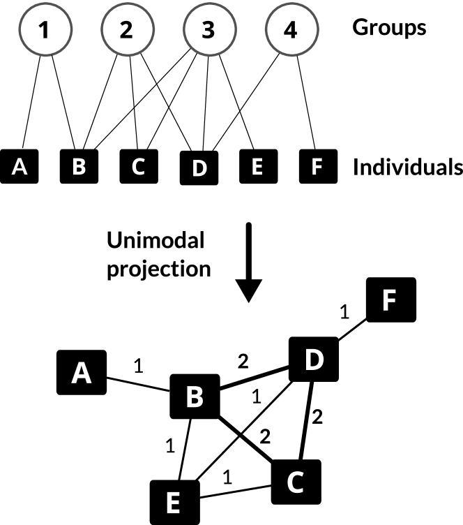
Figure 1:

Figure 2: Example of a co-occurrence network compiled from a bimodal entity-affiliation graph.

II Unweighted co-occurrence networks

Let us focus on the case where the link between a symbol and a set is unweighted, that is, a symbol either appears in a set or it doesn’t. We must formulate a randomization process whereby some set of meaningful and presumably robust features of the observed graph are preserved on average but the graph is randomized otherwise. We choose to preserve the degree sequences of both layers, one corresponding to the frequencies of the symbols throughout the data set, and the other corresponding to the size sequence of the sets to which the symbols can be related by membership. At first glance, this problem appears to be simply a bipartite analogue of the Marginal Likelihood Filter dianati_unwinding_2016 where for a given unimodal, integer-weighted event-counting network, a set of independent assignment events are distributed randomly between all possible node pairs such that the degree sequence is preserved on average. But the present problem is different for two reasons: 1) the inter-layer edges cannot be modified independently of one another since the co-membership relation is transitive, and 2) randomly distributing assignment events would allow for multiedges. We may then simply demand that a given pair $s_{i},u_{\alpha}$ be connected with probability $f_{i}g_{\alpha}/N$ which does indeed lead to the correct expectation value for both degrees. However, there is no guarantee that this quantity is even a probability. Instead, we derive a maximum entropy ensemble with the desired constraints, hoping to be able to compute the marginal probability distributions for all $(i,\alpha)$ edges, leading to a simple marginal significance test similar to dianati_unwinding_2016 .

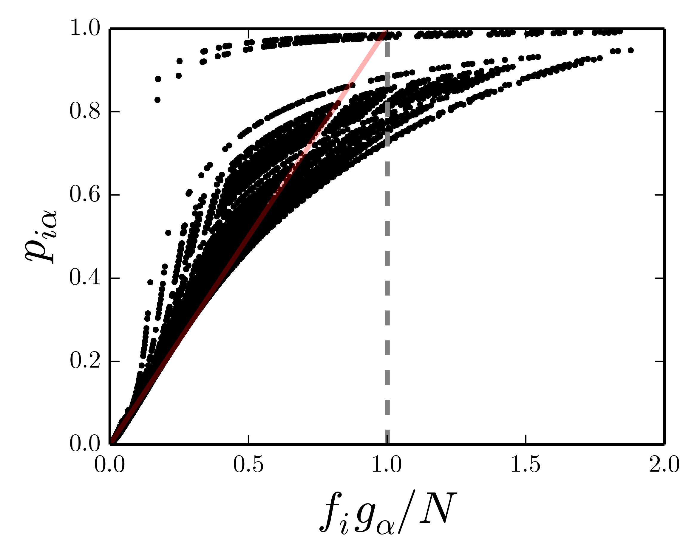
(a)

(b)

(c)

Figure 3: (a) The numerically computed connection probabilities between the two layers for the senate co-sponsorship network of the 110th US congress. Plotted against the “naive” probability. Note the highly nonlinear dependence. (b) Numerically solved $x_{i}y_{\alpha}$ as a function of the first order guess. In both plots, a cluster of points stand out, far above the bulk. These correspond to pairs with $g_{\alpha}\simeq n,$ i.e., sets that are connected to almost every entity, leading to near certain expected connectivity according to the null model. (c) p-value vs weight for edges in the co-occurrence graph.

Let us derive a maximum entropy graph ensemble that preserves both the set sizes $g_{\alpha}$ and symbol frequencies $f_{i}$ on average. The probability distribution for this ensemble is given by an exponential where our $m+n$ linear constraints $\left\langle\sum_{\alpha}\sigma_{i\alpha}\right\rangle=f_{i},\,\,i=1,2,\cdots m$ and $\left\langle\sum_{i}\sigma_{i\alpha}\right\rangle=g_{\alpha},\,\,\alpha=1,2,\cdots n$ are enforced by Lagrange multipliers $\lambda_{i},\,\,i=1,2,\cdots m$ and $\gamma_{\alpha},\,\,\alpha=1,2,\cdots n.$

$$P(G) \sim \exp\left[\sum_{i}\lambda_{i}\sum_{\alpha}\sigma_{i\alpha}+\sum_{\alpha}\gamma_{\alpha}\sum_{i}\sigma_{i\alpha}\right]$$ (2)

$$= \exp\left[\sum_{i,\alpha}\left(\lambda_{i}+\gamma_{\alpha}\right)\sigma_{i\alpha}\right]$$

where $\sigma_{i\alpha}$ is either zero or one, indicating whether nodes $i$ and $\alpha$ from the first and second layers respectively are connected. Therefore, the partition function is given by

$$Z = \sum_{\left\{\sigma_{i\alpha}\right\}}e^{\sum_{i,\alpha}\left(\lambda_{i}+\gamma_{\alpha}\right)\sigma_{i\alpha}}$$ (3)

$$= \sum_{\left\{\sigma_{i\alpha}\right\}}\prod_{i,\alpha}e^{\left(\lambda_{i}+\gamma_{\alpha}\right)\sigma_{i\alpha}}$$ (4)

$$= \prod_{i,\alpha}\left[1+e^{\left(\lambda_{i}+\gamma_{\alpha}\right)}\right].$$ (5)

Now we enforce the constraints and compute the Lagrange multipliers:

$$f_{j}=\frac{\partial\log Z}{\partial\lambda_{j}}\qquad\mbox{and}\qquad g_{\beta}=\frac{\partial\log Z}{\partial\gamma_{\beta}}.$$ (6)

Thus,

$$f_{j} =\sum_{\alpha}\frac{e^{\lambda_{j}+\gamma_{\alpha}}}{1+e^{\lambda_{i}+\gamma_{\alpha}}},$$ (7)

$$g_{\beta} =\sum_{i}\frac{e^{\lambda_{i}+\gamma_{\beta}}}{1+e^{\lambda_{i}+\gamma_{\beta}}}.$$ (8)

Defining $x_{i}=e^{\lambda_{i}}$ and $y_{\alpha}=e^{\gamma_{\alpha}},$ our problem is reduced to the solution of the following system of nonlinear equations:

$$y_{\alpha} = g_{\alpha}/\sum_{i}\frac{x_{i}}{1+x_{i}y_{\alpha}},\alpha=1,\cdots,n$$ (9)

$$x_{i} = f_{i}/\sum_{\alpha}\frac{y_{\alpha}}{1+x_{i}y_{\alpha}},i=1,\cdots,m.$$ (10)

Note that these equations are basically telling us that according to the maximum entropy scheme, the “occupation” probability of each of the possible edges between the first and second layers should have a logistic form:

$$p_{i\alpha}=\frac{e^{\lambda_{i}+\gamma_{\alpha}}}{1+e^{\lambda_{i}+\gamma_{\alpha}}}=\frac{x_{i}y_{\alpha}}{1+x_{i}y_{a}}.$$ (11)

III Solving the saddlepoint equations

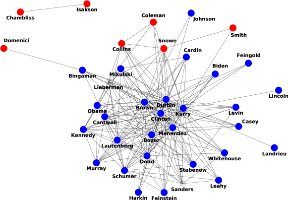
(a)

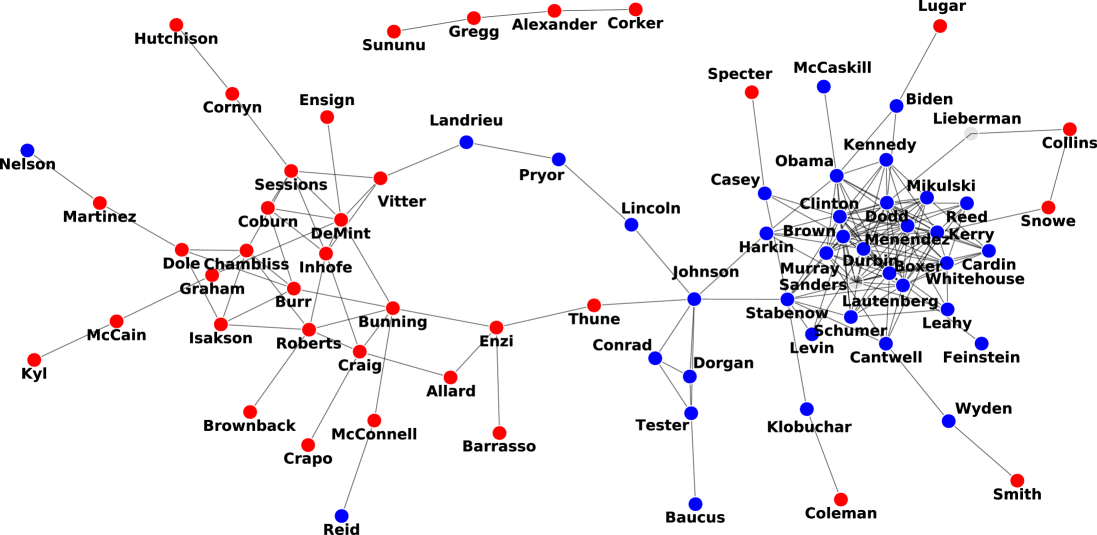
(b)

Figure 4: The two largest connected components of the US senate bill co-sponsorship network for the 110th congress, pruned down to network density 2 using a) weight thresholding, b) using our bimodal significance metric. Here, node colors indicate party membership.

It is not clear whether one can find a closed-form solution for equations (9) and (10). However, one can solve them numerically using iterative methods. In (9) and (10) we have already written the system of the equations in the form:

$$x_{i}=\phi_{i}(\left\{x_{j}\right\},\left\{y_{\beta}\right\}),\quad y_{\alpha}=\psi_{\alpha}(\left\{x_{j}\right\},\left\{y_{\beta}\right\}).$$ (12)

The solution is therefore the fixed point of the system of transformations defined by $\phi_{i},i=1,\cdots,m$ and $\psi_{\alpha},\alpha=1,\cdots n.$ In order to compute the fixed point, we start with initial guesses for each of the $x_{i}$ and $y_{\alpha}$ and iterate the following equations until convergence:

$$x_{i}^{[k+1]}=\phi_{i}\left(\left\{x_{j}^{[k]}\right\},\left\{y_{\beta}^{[k]}\right\}\right),$$ (13)

$$y_{\alpha}^{[k+1]}=\psi_{\alpha}\left(\left\{x_{j}^{[k]}\right\},\left\{y_{\beta}^{[k]}\right\}\right)$$ (14)

where the superscript indexes the current step in the iteration. As the initial values, we use $x_{i}=f_{i}/\sqrt{N}$ and $y_{\alpha}=g_{\alpha}/\sqrt{N}$ which correspond to the first order solution in terms of $x_{i}y_{\alpha}.$ Figure 3 shows the results from the numerical solution of these equations for the US senate cosponsorship data with $m=3613,$ $n=102,$ such that the co-occurrence graph has 5151 edges. For details of this data and further discussion, see section VI.

IV Co-occurrence network

Having computed the null model’s inter-layer connection probabilities, we now proceed to derive the probability distribution for the co-occurrence weight of pairs of symbols (first layer nodes). The quantity of interest is the probability distribution for the random variables $M(s_{i},s_{j})$ defined as follows:

$$M(s_{i},s_{j}): =$$ number of nodes in the second

layer linked both to $$s_{i} s_{j}.$$ and

The expectation value of this random variable is given by

$$\mathbb{E}\left[M(s_{i},s_{j})\right] = \sum_{\alpha=1}^{n}p_{i\alpha}p_{j\alpha}$$ (16)

If $x_{i}\neq x_{j},$ the summand simplifies to

$$p_{i\alpha}p_{j\alpha} = \frac{x_{i}x_{j}y_{\alpha}}{x_{i}-x_{j}}\left[\frac{1}{1+x_{j}y_{\alpha}}-\frac{1}{1+x_{i}y_{\alpha}}\right]$$ (17)

and thus, the sum over $\alpha$ becomes

$$\mathbb{E}\left[M(s_{i},s_{j})\right] =\sum_{\alpha}p_{i\alpha}p_{j\alpha}=\frac{1}{x_{i}-x_{j}}\left[x_{i}f_{j}-x_{j}f_{i}\right]$$

$$\mbox{for }x_{i}\neq x_{j}.$$ (18)

If $x_{i}=x_{j},$ however, this simplification is not valid and we must compute the full sum

$$\mathbb{E}\left[M(s_{i},s_{j})\right] =\sum_{\alpha}p_{i\alpha}p_{j\alpha}=\sum_{\alpha}\frac{x_{i}^{2}y_{\alpha}^{2}}{\left(1+x_{i}y_{\alpha}\right)^{2}}$$

$$\mbox{for}\,x_{i}=x_{j}.$$ (19)

Similarly, we may compute the variance:

$$\operatorname{Var}\left[M(s_{i},s_{j})\right]=\sum_{\alpha}p_{i\alpha}p_{j\alpha}(1-p_{i\alpha}p_{j\alpha}).$$ (20)

Using these expressions we compute and store $\mathbb{E}\left[M(s_{i},s_{j})\right]$ and $\operatorname{Var}\left[M(s_{i},s_{j})\right]$ once for every edge in the observed graph. This operation has time complexity $O(n\left|E\right|)$ where $\left|E\right|$ is the size of the edge set of the co-occurence network.

V Distribution of the co-occurrence weights

The final step is to estimate the probability distribution of $M(s_{i},s_{j})$ so that a p-value may be computed for each edge. Note that $M(s_{i},s_{j})$ is the sum of $n$ binary indicator variables each indicating whether $s_{i}$ and $s_{j}$ “co-occurred” in a set $u_{\alpha}.$ Therefore, for large $n,$ by the central limit theorem, we expect the distribution to approach a normal distribution. However, in general this approximation does not yield accurate results. To be precise, the sum of independent and different Bernoulli variables is known as the Poisson binomial distribution. Simple closed form expressions of the pdf and cdf for this distribution aren’t known, but various approximations as well as exact, albeit computationally expensive numerical estimation methods are known FernandezPoissonBinom ; Hong201341 . Here we use the so-called refined normal approximation (RNA) due to Volkova volkova_refinement_1996 which is a modification of the normal approximation. See Appendix A for details.

Given the cdf $F_{ij}(k)$ for the null distribution of the weight between nodes $i,j$ in the co-occurrence graph and an observed weight $w_{ij}$, we compute the pvalue $\pi_{ij}$

$$\pi_{ij}(w_{ij})=1-F_{ij}(w_{ij})$$ (21)

and define the significance metric as $-\log(\pi_{ij}(w_{ij})).$

VI Application to data

In this section we present the results of the application of the filter to the senate bill cosponsorship in the 110th US congress (2007-2008). The data is from fowler_connecting_2006 ; fowler_legislative_2006 and contains a list of all bills introduced in the senate and for each one, the list of senators who cosponsored the bill. Aside from its original sponsor, a bill can also be cosponsored by an arbitrary number of other senators. Senators cosponsor bills for a variety of reasons, including partisan allegiance, lending support and forming strategic alliances, and simply increasing their own visibility and perceived political clout. Regardless, being cosponsors of a given bill is a signal of affinity as regards the legislative process. The data then consists of a bipartite graph where the nodes represent the senators in the first layer and the bills in the second layer and an inter-layer link indicates cosponsorship of a bill by a senator. The co-sponsorhip network is then the projection of this bipartite graph onto the first layer. The full co-occurence network consists of 102 nodes and more than 5000 edges, a rather dense graph with no visible structure. Figure 4 shows this network pruned using naive weight thresholding as well as our significance measure. Each graph shows the giant component as well as the next largest connected component of the graph after it is pruned down to network density 2 using each pruning scheme. The graph on the left shows a cluster of mostly Democrats with the rest of the graph more or less disintegrated. The one on the right on the other hand, shows most of the nodes connected through the giant component, which demonstrates a highly modular community structure reflecting the main partisan division with the senate. Both figures are rendered using the Kamada-Kawai graph layout, a popular force directed layout algorithm. Figure 5 compares weight thresholding and the bimodal filter. On the left, the size of the giant components truncated at various network densities are compared. With our significance measure, the giant component already contains about 80% of all the nodes at density 2 and nearly all at density 4, whereas weight thresholding leaves the graph rather disintegrated up to high densities: a rather small giant component, with the rest of the nodes scattered across singletons and otherwise very small components. The figure on the right compares the two methods in terms of their ability to reveal the partisan divide within the senate. Given the known party memberships of US senators, we computed the modularity scores of the pruned graphs at different truncation levels, both for weight thresholding as well as our bimodal filtering technique. The modularity of graphs resulting from our filtering technique is consistently and significantly higher than those produced by weight thresholding, showing that the partisan divide is manifest much more clearly with the application of our filter.

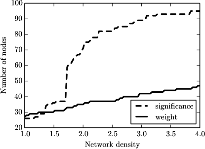
(a)

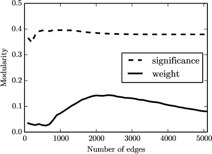
(b)

Figure 5: a) The size of the giant component for the US senate co-sponsorship network pruned down to various network densities using the bimodal significance measure as well as weight thresholding. b) The modularity of the same networks according to party membership.

Appendix A Refined normal approximation

In this appendix we describe the refined normal approximation for the cdf of the Poisson binomial distribution due to Volkova volkova_refinement_1996 . For the sum of $n$ independent Bernoulli random variables with means $p_{i,}\,i=1,2,\cdots n,$ The cdf, $F(k)$ is approximately given by

$$F(k)\approx G\left(\frac{k+0.5-\mu}{\sigma}\right),k=0,1,\cdots,n$$ (22)

where

$$G(x)=\Phi(x)+\gamma(1-x^{2})\phi(x)/6,$$ (23)

$\phi(x)$ ,$\Phi(x)$ are the pdf and cdf of the standard normal distribution respectively and

$$\gamma=\sigma^{-3}\eta\,\,\mbox{where}\,\,\eta=\sum_{j=1}^{n}p_{j}(1-p_{j})(1-2p_{j})$$ (24)

So, the ingredients necessary for this computation are the following:

$$\mu = \sum_{i=1}^{n}p_{i}$$ (25)

$$\sigma^{2} = \sum_{i=1}^{n}p_{i}(1-p_{i})$$ (26)

$$\eta = \sum_{i=1}^{n}p_{j}(1-p_{j})(1-2p_{j})$$ (27)

$$\phi(x) = \frac{1}{\sqrt{2\pi}}e^{-x^{2}/2}$$ (28)

$$\Phi(x) = \frac{1}{2}\left[1+\operatorname{erf}\left(\frac{x}{\sqrt{2}}\right)\right]$$ (29)

References

- (1) A. Davis, B. B. Gardner, and M. R. Gardner, Deep South: A social anthropological study of caste and class. Univ of South Carolina Press, 2009.
- (2) D. J. Watts and S. H. Strogatz, “Collective dynamics of ’small-world’networks,” nature, vol. 393, no. 6684, pp. 440–442, 1998.
- (3) J. H. Fowler, “Connecting the congress: A study of cosponsorship networks,” Political Analysis, vol. 14, no. 4, pp. 456–487, 2006.
- (4) J. H. Fowler, “Legislative cosponsorship networks in the us house and senate,” Social Networks, vol. 28, no. 4, pp. 454–465, 2006.
- (5) M. Á. Serrano, M. Boguñá, and A. Vespignani, “Extracting the multiscale backbone of complex weighted networks,” Proceedings of the National Academy of Sciences, vol. 106, pp. 6483–6488, Apr. 2009.
- (6) F. Radicchi, J. Ramasco, and S. Fortunato, “Information filtering in complex weighted networks,” Physical Review E, vol. 83, p. 046101, Apr. 2011.
- (7) N. Dianati, “Unwinding the hairball graph: Pruning algorithms for weighted complex networks,” Physical Review E, vol. 93, p. 012304, Jan. 2016.
- (8) M. Latapy, C. Magnien, and N. D. Vecchio, “Basic notions for the analysis of large two-mode networks,” Social Networks, vol. 30, no. 1, pp. 31 – 48, 2008.
- (9) Z. Neal, “The backbone of bipartite projections: Inferring relationships from co-authorship, co-sponsorship, co-attendance and other co-behaviors,” Social Networks, vol. 39, pp. 84–97, Oct. 2014.
- (10) M. Fernandez and S. Williams, “Closed-form expression for the poisson-binomial probability density function,” IEEE Transactions on Aerospace and Electronic Systems, vol. 46, pp. 803–817, April 2010.
- (11) Y. Hong, “On computing the distribution function for the poisson binomial distribution,” Computational Statistics & Data Analysis, vol. 59, pp. 41 – 51, 2013.
- (12) A. Y. Volkova, “A Refinement of the Central Limit Theorem for Sums of Independent Random Indicators,” Theory of Probability & Its Applications, vol. 40, no. 4, pp. 791–794, 1996.
- (13) J. H. Fowler, “Connecting the Congress: A Study of Cosponsorship Networks,” Political Analysis, vol. 14, pp. 456–487, Sept. 2006.
- (14) J. H. Fowler, “Legislative cosponsorship networks in the US House and Senate,” Social Networks, vol. 28, pp. 454–465, Oct. 2006.