Rolling Horizon Coevolutionary Planning for Two-Player Video Games

Abstract

This paper describes a new algorithm for decision making in two-player real-time video games. As with Monte Carlo Tree Search, the algorithm can be used without heuristics and has been developed for use in general video game AI.

The approach is to extend recent work on rolling horizon evolutionary planning, which has been shown to work well for single-player games, to two (or in principle many) player games. To select an action the algorithm co-evolves two (or in the general case $N$) populations, one for each player, where each individual is a sequence of actions for the respective player. The fitness of each individual is evaluated by playing it against a selection of action-sequences from the opposing population. When choosing an action to take in the game, the first action is chosen from the fittest member of the population for that player.

The new algorithm is compared with a number of general video game AI algorithms on three variations of a two-player space battle game, with promising results.

I Introduction

Since the dawn of computing, games have provided an excellent test bed for AI algorithms, and increasingly games have also been a major AI application area. Over the last decade progress in game AI has been significant, with Monte Carlo Tree Search dominating many areas since 2006[1, 2, 3, 4, 5], and more recently deep reinforcement learning has provided amazing results, both in stand-alone mode in video games, and in combination with MCTS in the shape of AlphaGo[6], which achieved one of the greatest steps forward in a mature and competitive area of AI ever seen. AlphaGo not only beat Lee Sedol, previous world Go champion, but also soundly defeated all leading Computer Go bots, many of which had been in development for more than a decade. Now AlphaGo is listed at the second position among current strongest human players.

With all this recent progress a distant observer could be forgiven for thinking that Game AI was starting to become a solved problem, but with smart AI as a baseline the challenges become more interesting, with ever greater opportunities to develop games that depend on AI either at the design stage or to provide compelling gameplay.

The problem addressed in this paper is the design of general algorithms for two-player video games. As a possible solution, we introduce a new algorithm: Rolling Horizon Coevolution Algorithm (RHCA). This only works for cases when the forward model of the game is known and can be used to conduct what-if simulations (roll-outs) much faster than real time. In terms of the General Video Game AI (GVGAI) competition series, this is known as the two-player planning track[7]. However, this track was not available at the time of writing this paper, so we were faced with the choice of using an existing two-player video game, or developing our own. We chose to develop our own set simple battle game, bearing some similarity to the original 1962 Spacewar game though lacking the fuel limit and the central death star with the gravity field. This approach provides direct control over all aspects of the game and enables us to optimise it for fast simulations, and also to experiment with parameters to test the generality of the results.

The two-player planning track is interesting because it offers the possibility of AI which can be instantly smart with no prior training on a game, unlike Deep Q Learning (DQN) approaches [8] which require extensive training before good performance can be achieved. Hence the bots developed using our planning methods can be used to provide instant feedback to game designers on aspects of gameplay such as variability, challenge and skill depth.

The most obvious choice for this type of AI is Monte Carlo Tree Search (MCTS), but recent results have shown that for single-player video games, Rolling Horizon Evolutionary Algorithms (RHEA) are competitive. Rolling horizon evolution works by evolving a population of action sequences, where the length of each sequence equals the depth of simulation. This is in contrast to MCTS where by default (and for reasons of efficiency, and of having enough visits to a node to make the statistics informative) the depth of tree is usually shallower than the total depth of the rollout (from root to the final evaluated state).

The use of action-sequences rather than trees as the core unit of evaluation has strengths and weaknesses. Strengths include simplicity and efficiency, but the main weakness is that the individual sequence-based approach would by default ignore the savings possible by recognising shared prefixes, though prefix-trees can be constructed for evaluation purposes if it is more efficient to do so[9]. A further disadvantage is that the system is not directly utilising tree statistics to make more informed decisions, though given the limited simulation budget typically available in a real-time video game, the value of these statistics may be outweighed by the benefits of the rolling horizon approach.

Given the success of RHEA on single-player games, the question naturally arises of how to extend the algorithm to two-player games (or in the general case $N$-player games), with the follow-up question of how well such an extension works. The main contributions of this paper are the algorithm, RHCA, and the results of initial tests on our two-player battle game. The results are promising, and suggest that RHCA could be a natural addition to a game AI practitioner’s toolbox.

The rest of this paper is structured as follows: Section II provides more background to the research, Section III describes the battle games used for the experiments, Section IV describes the controllers used in the experiments, Section V presents the results and Section VI concludes.

II Background

II-A Open Loop control

Open loop control refers to those techniques which action decision mechanism is based on executing sequences of actions determined independently from the states visited during those sequences. Weber discusses the difference between closed and open loop in [10]. An open loop technique, Open Loop Expectimax Tree Search (OLETS), developed by Couëtoux, won the first GVGAI competition in 2014 [7], an algorithm inspired by Hierarchical Open Loop Optimistic Planning (HOLOP, [11]). Also in GVGAI, Perez et al. [9] discussed three different open loop techniques, then trained them on 28 games of the framework, and tested on 10 games.

The classic closed loop tree search is efficient when the game is deterministic, i.e., given a state $s$, $\forall a\in A(s)$ ($A(s)$ is the set of legal actions in $s$), the next state $s^{\prime}\leftarrow S(a,s)$ is unique. In the stochastic case, given a state $s$, $\forall a\in A(s)$ ($A(s)$ is the set of legal actions in $s$), the state $s^{\prime}\leftarrow S(a,s)$ is drawn with a probability distribution from the set of possible future states.

II-B Rolling Horizon planning

Rolling Horizon planning, sometimes called Receding Horizon Control or Model Predictive Control (MPC), is commonly used in industries for making decisions in a dynamic stochastic environment. In a state $s$, an optimal input trajectory is made based on a forecast of the next $t_{h}$ states, where $t_{h}$ is the tactical horizon. Only the first input of the trajectory is applied to the problem. This procedure repeats periodically with updated observations and forecasts.

A rolling horizon version of an Evolutionary Algorithm that handles macro-actions was applied to the Physical Traveling Salesman Problem (PTSP) as introduced in [12]. Then, RHEA was firstly applied on general video game playing by Perez et al. in [9] and was shown to be the most efficient evolutionary technique on the GVGAI Competition framework.

III Battle games

Our two-player space battle game could be viewed as derived from the original Spacewar (as mentioned above). We then experimented with a number of variations to bring out some strengths and weaknesses of the various algorithms under test. A key finding is that the rankings of the algorithms depend very much on the details of the game; had we just tested on a single version of the game the conclusions would have been less robust and may have shown RHCA in a false light. The agents are given full information about the game state and make their actions simultaneously: the games are symmetric with perfect and incomplete information. Each game commences with the agents in random symmetric positions to provide varied conditions while maintaining fairness.

III-A A simple battle game

First, a simple version without missiles is designed, referred as $G_{1}$. Each spaceship, either owned by the first (green) or second (blue) player has the following properties:

• has a maximal speed equals to $3$ units distance per game tick;

• slows down over time;

• can make a clockwise or anticlockwise rotation, or to thrust at each game tick.

Thus, the agents are in a fair situation.

III-A1 End condition

A player wins the game if it faces to the back of its opponent in a certain range before the total game ticks are used up. Figure 1 illustrates how the winning range is defined. If no one wins the game when the time is elapsed, it’s a draw.

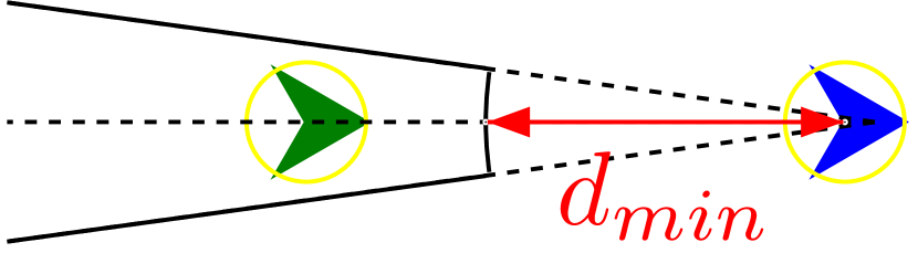
Figure 1: The area in the bold black curves defines the ”winning” range with $d_{min}=100$ and $cos(\alpha/2)=0.95$. This is a win for the green player.

III-A2 Game state evaluation

Given a game state $s$, if a ship $i$ is located in the predefined winning range (Fig. 1), the player gets a score $DistScore_{i}=HIGH\_VALUE$ and the winner is set to $i$; otherwise, $DistScore_{i}=\frac{100}{dot+100}$ ($\in(0,1]$), where $dot_{i}$ is the scalar product of the vector from the ship $i$’s position to its opponent and the vector from its direction to its opponent’s direction. The position and direction of both players are taken into account to direct the trajectory.

III-B Perfect and incomplete information

The battle game and its variants have perfect information, because each agent knows all the events (e.g. position, direction, life, speed, etc. of all the objects on the map) that have previously occurred when making any decision; they have incomplete information because neither of agents knows the type or strategies of its opponent and moves are made simultaneously.

IV Controllers

In this section, we summarize the different controllers used in this work. All controllers use the same heuristic to evaluate states (Section IV-A).

IV-A Search Heuristic

All controllers presented in this work follow the same heuristic in the experiments where a heuristic is used (Algorithm 1), aiming at guiding the search and evaluating game states found during the simulations. The end condition of the game is checked (detailed in Section III-A1) at every tick. When a game ends, a player may have won or lost the game or there is a draw. In the former two situations, a very high positive value or low negative value is assigned to the fitness respectively. A draw only happens at the end of last tick.

Algorithm 1 Heuristic.

1:function EvaluateState(State $s$, Player $p1$, Player $p2$)

2:     $fitness_{1}\leftarrow 0$, $fitness_{2}\leftarrow 0$

3:     $s\leftarrow Update(p1,p2)$

4:     if $Winner(s)==1$ then

5:         $fitness_{1}\leftarrow HIGH\_VALUE$

6:     else

7:         $fitness_{1}\leftarrow LOW\_VALUE$

8:     end if

9:     if $Winner(s)==2$ then

10:         $fitness_{2}\leftarrow HIGH\_VALUE$

11:     else

12:         $fitness_{2}\leftarrow LOW\_VALUE$

13:     end if

14:     if $Winner(s)==null$ then

15:         $fitness_{1}\leftarrow Score_{1}(s)-Score_{2}(s)$

16:         $fitness_{2}\leftarrow Score_{2}(s)-Score_{1}(s)$

17:     end if

18:     return $fitness_{1}$, $fitness_{2}$

19:end function

IV-B RHEA Controllers

In the experiments described later in Section V, two controllers implement a distinct version of rolling horizon planning: the Rolling Horizon Genetic Algorithm (RHGA) and Rolling Horizon Coevolutionary Algorithm (RHCA) controllers. These two controllers are defined next.

IV-B1 Rolling Horizon Genetic Algorithm (RHGA)

In the experiments described later in Section V, this algorithm uses truncation selection with arbitrarily chosen threshold $20$, i.e., the $20\%$ best individuals will be selected as parents. The pseudo-code of this procedure is given in Algorithm 2.

Algorithm 2 Rolling Horizon Genetic Algorithm (RHGA)

1:$\lambda\in{\mathbb{N}}^{*}$: population size, $\lambda>2$

2:$ProbaMut\in(0,1)$: mutation probability

3:Randomly initialise population $\mathbf{x}$ with $\lambda$ individuals

4:Randomly initialise opponent’s individual $y$

5:for $x\in\mathbf{x}$ do

6:     Evaluate the fitness of $x$ and $y$

7:end for

8:Sort $\mathbf{x}$ by decreasing fitness value order, so that

$$x_{1}.fitness\geq x_{2}.fitness\geq\cdots$$

9:while time not elapsed do

10:     Randomly generate $y$ $\triangleright$ Update opponent’s individual

11:     $x^{\prime}_{1}\leftarrow x_{1}$, $x^{\prime}_{2}\leftarrow x_{2}$ $\triangleright$ Keep stronger individuals

12:     for $k\in\{3,\dots,\lambda\}$ do $\triangleright$ Offspring

13:         Generate $x^{\prime}_{k}$ from $x^{\prime}_{1}$ and $x^{\prime}_{2}$ by uniform crossover

14:         Mutate $x^{\prime}_{k}$ with probability $ProbMut$

15:     end for

16:     $\mathbf{x}\leftarrow\mathbf{x^{\prime}}$ $\triangleright$ Update population

17:     for $x\in\mathbf{x}$ do

18:         Evaluate the fitness of $x$ and $y$

19:     end for

20:     Sort $\mathbf{x}$ by decreasing fitness value order, so that

$$x_{1}.fitness\geq x_{2}.fitness\geq\cdots$$

21:end while

22:return $x_{1}$, the best individual in $\mathbf{x}$

IV-B2 Rolling Horizon Coevolutionary Algorithm (RHCA)

RHCA (Algorithm 3) uses a tournament-based truncation selection with threshold $20$ and two populations $\mathbf{x}$ and $\mathbf{y}$, where each individual in $\mathbf{x}$ represents some successive behaviours of current player and each individual in $\mathbf{y}$ represents some successive behaviours of its opponent. The objective of $\mathbf{x}$ is to evolve better actions to kill the opponent, whereas the objective of $\mathbf{y}$ is to evolve stronger opponents, thus provide a worse situation to the current player. At each generation, the best $2$ individuals in $\mathbf{x}$ (respectively $\mathbf{y}$) are preserved as parents (elites), afterwards the rest is generated using the parents by uniform crossover and mutation. Algorithm 4 is used to evaluate game state, given two populations, then sort both populations by average fitness value. Only a subset of the second population is involved.

Algorithm 3 Rolling Horizon Coevolutionary Algorithm (RHCA)

1:$\lambda\in{\mathbb{N}}^{*}$: population size, $\lambda>2$

2:$ProbaMut\in(0,1)$: mutation probability

3:$SubPopSize$: the number of selected individuals from opponent’s population

4:$\textsc{EvaluateAndSort}($)

5:Randomly initialise population $\mathbf{x}$ with $\lambda$ individuals

6:Randomly initialise opponent’s population $\mathbf{y}$ with $\lambda$ individuals

7:$(\mathbf{x},\mathbf{y})\leftarrow\textsc{EvaluateAndSort}(\mathbf{x},\mathbf{y},SubPopSize)$

8:while time not elapsed do

9:     $y^{\prime}_{1}\leftarrow y_{1}$, $y^{\prime}_{2}\leftarrow y_{2}$ $\triangleright$ Keep stronger rivals

10:     for $k\in\{3,\dots,\lambda\}$ do $\triangleright$ Opponent’s offspring

11:         Generate $y^{\prime}_{k}$ from $y^{\prime}_{1}$ and $y^{\prime}_{2}$ by uniform crossover

12:         Mutate $y^{\prime}_{k}$ with probability $ProbMut$

13:     end for

14:     $\mathbf{y}\leftarrow\mathbf{y^{\prime}}$ $\triangleright$ Update opponent’s population

15:     $x^{\prime}_{1}\leftarrow x_{1}$, $x^{\prime}_{2}\leftarrow x_{2}$ $\triangleright$ Keep stronger individuals

16:     for $k\in\{3,\dots,\lambda\}$ do $\triangleright$ Offspring

17:         Generate $x^{\prime}_{k}$ from $x^{\prime}_{1}$ and $x^{\prime}_{2}$ by uniform crossover

18:         Mutate $x^{\prime}_{k}$ with probability $ProbMut$

19:     end for

20:     $\mathbf{x}\leftarrow\mathbf{x^{\prime}}$ $\triangleright$ Update population

21:     $EvaluateAndSort(\mathbf{x},\mathbf{y},SubPopSize)$

22:end while

23:return $x_{1}$, the best individual in $\mathbf{x}$

Algorithm 4 Evaluate fitness of population and subset of another population then sort the populations.

function EvaluateAndSort(population $\mathbf{x}$, population $\mathbf{y}$, $SubPopSize\in{\mathbb{N}}^{*}$)

     for $x\in\mathbf{x}$ do

         for $i\in\{1,\dots,SubPopSize\}$ do

              Randomly select $y\in\mathbf{y}$

              Evaluate the fitness of $x$ and $y$ once, update their average fitness value

         end for

     end for

     Sort $\mathbf{x}$ by decreasing average fitness value order, so that

$$x_{1}.averageFitness\geq x_{2}.averageFitness\geq\cdots$$

     Sort $\mathbf{y}$ by decreasing average fitness value order, so that

$$y_{1}.averageFitness\geq y_{2}.averageFitness\geq\cdots$$

return $(\mathbf{x},\mathbf{y})$

end function

IV-B3 Macro-actions and single actions

A macro-action is the repetition of the same action for $t_{o}$ successive time steps. Different values of $t_{o}$ are used during the experiments in this work in order to show how this parameter affects the performance. The individuals in both algorithms have genomes with length equals to the number of future actions to be optimised, i.e., $t_{h}$.

In all games, different numbers of actions per macro-action are considered in RHGA and RHCA. The first results show that there is an improvement in performance, for all games, the shorter the macro-action is. The result using one action per macro-action, i.e., $t_{o}=1$, will be presented.

Recommendation policy In both algorithms, the recommended trajectory is the individual with highest average fitness value in the population (Algorithm 2 line 22; Algorithm 3 line 23). The first action in the recommended trajectory, presented by the gene at position $1$, is the recommended action in the next single time step.

IV-C Open Loop MCTS

A Monte Carlo Tree Search (MCTS) using Open Loop control (OLMCTS) is included in the experimental study. This was adapted from the OLMCTS sample controller included in the GVGAI distribution [13]. The OLMCTS controller was developed for single player games, and we adapted it for two player games by assuming a randomly acting opponent. Better performance should be expected of a proper two-player OLMCTS version using a minimax (more max-N) tree policy and immediate future work is to evaluate such an agent.

Recommendation policy The recommended action in the next single time step is the one present in the most visited root child, i.e., robust child[1]. If more than one child ties as the most visited, the one with the highest average fitness value is recommended.

IV-D One-Step Lookahead

One-Step Lookahead algorithm (Algorithm 5) is deterministic. Given a game state $s$ at timestep $t$ and the sets of legal actions of both players $A(s)$ and $A^{\prime}(s)$, One-Step Lookahead algorithm evaluates the game then outputs an action $a_{t+1}$ for the next single timestep using some recommendation policy.

Algorithm 5 One-Step Lookahead algorithm.

1:$s$: current game state

2:$Score$: score function

3:$\pi$: recommendation policy

4:Generate $A(s)$ the set of legal actions for player 1 in state $s$

5:Generate $A^{\prime}(s)$ the set of legal actions for player 2 in state $s$

6:for $i\in\{1,\dots,|A(s)|\}$ do

7:     for $j\in\{1,\dots,|A^{\prime}(s)|\}$ do

8:         $a_{i}\leftarrow i^{th}$ action in $A$

9:         $a_{j}\leftarrow j^{th}$ action in $A^{\prime}$

10:         $M_{i,j}\leftarrow Score_{1}(s,a_{i},a^{\prime}_{j})$

11:         $M^{\prime}_{i,j}\leftarrow Score_{2}(s,a_{i},a^{\prime}_{j})$

12:     end for

13:end for

14:$\tilde{a}\leftarrow\pi$, using $M$ or $M^{\prime}$ or both

15:return $\tilde{a}$: recommended action

Recommendation policy There are various choices of $\pi$, such as Wald [14] and Savage [15] criteria. Wald consists in optimizing the worst case scenario, which means that we choose the best solution for the worst scenarios. Thus, the recommended action for player 1 is

$$\tilde{a}=\operatorname*{arg\,max}_{i\in\{1,\dots,|A(s)|\}}\min_{j\in\{1,\dots,|A^{\prime}(s)|\}}M_{i,j}.$$ (1)

Savage is an application of the Wald maximin model to the regret:

$$\tilde{a}=\operatorname*{arg\,min}_{i\in\{1,\dots,|A(s)|\}}\max_{j\in\{1,\dots,|A^{\prime}(s)|\}}M^{\prime}_{i,j}.$$ (2)

We also include a simple policy which chooses the action with maximal average score, i.e.,

$$\tilde{a}=\operatorname*{arg\,max}_{i\in\{1,\dots,|A(s)|\}}\sum_{j\in\{1,\dots,|A^{\prime}(s)|\}}M_{i,j}.$$ (3)

Respectively,

$$\tilde{a}=\operatorname*{arg\,min}_{i\in\{1,\dots,|A(s)|\}}\sum_{j\in\{1,\dots,|A^{\prime}(s)|\}}M^{\prime}_{i,j}.$$ (4)

The OneStep controllers use separately (1) Wald (Equation 1) on its score; (2) maximal average score (Equation 3) policy; (3) Savage (Equation 1); (4) minimal the opponent’s average score (Equation 4); (5) Wald on (its score - the opponent’s score) and (6) maximal average (its score - the opponent’s score). In the experiments described in Section V we only present the results obtained by using (6), which performs the best among the 6 policies.

V Experiments on battle games

We compare a RHGA controller, a RHCA controller, an Open Loop MCTS controller and an One-Step Lookahead controller, a move in circle controller and a rotate-and-shoot controller, denoted as RHGA, RHCA, OLMCTS, OneStep, ROT and RAS respectively, by playing a two-player battle game of perfect and incomplete information.

V-A Parameter setting

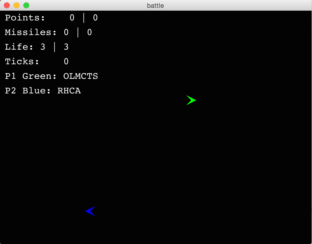
Figure 2: At the beginning of every game, each spaceship is randomly initialised with a back-to-back position.

All controllers should decide an action within $10ms$. OLMCTS uses a maximum depth$=10$. Both RHCA and RHGA have a population size $\lambda=10$, $ProbaMut=0.3$ and $t_{h}=10$. The size of sub-population used in tournament ($SubPopSize$ in Algorithm 3) is set to $3$. These parameters are arbitrarily chosen. Games are initialised with random positions of spaceships and opposite directions (cf. Figure 2).

V-B Analysis of numerical results

We measure a controller by the number of wins and how quickly it achieves a win. Controllers are compared by playing games with each other using the full round-robin league. As the game is stochastic (due to the random initial positions of ships, the random process included in recoil or hitting), several games with random initialisations are played between any pair of the controllers.

A rotated controller, denoted as ROT, is also compared. For comparison, a random controller, denoted as RND, is included in all the battle games.

Table I illustrates the experimental results.

TABLE I: Analysis of the number of wins of the line controller against the column controller in the battle games described in Section III-A. The more wins achieved, the better controller performs. $10ms$ is given at each game tick and $MaxTick=2000$. Each game is repeated $100$ times with random initialization. $RHCA$ outperforms all the controllers.

Test case 1: Simple battle game without weapon ($G_{1}$).
	RND	ROT	OneStep	OLMCTS	$RHCA$	$RHGA$	Avg.
RND	-	62.5	51.0	9.0	6.5	7.5	27.3
RAS	37.5	-	0.0	0.0	0.0	0.0	7.5
OneStep	49.0	100.0	-	49.5	13.0	42.0	50.7
OLMCTS	91.0	100.0	50.5	-	50.0	50.0	68.3
$RHCA$	93.5	100.0	87.0	50.0	-	50.0	76.1
$RHGA$	92.5	100.0	58.0	50.0	50.0	-	70.1
Avg.	72.7	92.5	49.3	31.7	23.9	29.9

Every entry in the table presents the number of wins of the column controller against the line controller among $100$ trials of battle games. The number of wins is calculated as follows: for each trial of game, if it’s a win of the column controller, the column controller accumulates $1$ point, if it’s a loss, the line controller accumulates $1$ point; otherwise, it’s a draw, both column and line controllers accumulates $0.5$ point.

V-B1 ROT

The rotated controller ROT, which goes in circle, is deterministic and vulnerable in simple battle games.

V-B2 RND

The RND controller is not outstanding in the simple battle game.

V-B3 OneStep

OneStep is feeble in all games against all the other controllers except one case: against ROT in $G_{1}$. It’s no surprise that OneStep beats ROT, a deterministic controller, in all the $100$ trials of $G_{1}$. Among the $100$ trials of $G_{1}$, OneStep is beaten separately by OLMCTS once and RND twice, the other trials finish by a draw. This explains the high standard error.

V-B4 OLMCTS

OLMCTS outperforms ROT and RND, however, there is no clear advantage or disadvantage when against OneStep, RHCA or RHGA.

V-B5 RHCA

In all the games, the less actions set in a macro-action, the better RHCA performs. RHCA outperforms all the controllers.

V-B6 RHGA

In all the games, the less actions set in a macro-action, the better RHGA performs. RHGA is the second-best in the battle game.

VI Conclusions and further work

In this work, we design a new Rolling Horizon Coevolutionary Algorithm (RHCA) for decision making in two-player real-time video games. This algorithm is compared to a number of general algorithms on the simple battle game designed, and some more difficult variants to distinguish the strength of the compared algorithms. In all the games, more actions per macro-action lead to a worse performance of both Rolling Horizon Evolutionary Algorithms (controllers denoted as RHGA and RHCA in the experimental study). Rolling Horizon Coevolution Algorithm (RHCA) is found to perform the best or second-best in all the games.

More work on battle games with weapon is in progress. In the battle game, the sum of two players’ fitness value remains 0. An interesting further work is to use a mixed strategy by computing Nash Equilibrium[16]. Furthermore, a Several-Step Lookahead controller is used to recommend the action at next tick, taken into account actions in the next $n$ ticks. A One-Step Lookahead controller is a special case of Several-Step Lookahead controller with $n=1$. As the computational time increases exponentially as a function of $n$, some adversarial bandit algorithms may be included to compute an approximate Nash[17] and it would be better to include some infinite armed bandit technique.

Finally, it is worth emphasizing that rolling horizon evolutionary algorithms provide an interesting alternative to MCTS that has been very much under-explored. In this paper we have taken some steps to redress this with initial developments of a rolling horizon coevolution algorithm. The algorithm described here is a first effort and while it shows significant promise, there are many obvious ways in which it can be improved, such as biasing the roll-outs [18]. In fact, any of the techniques that can be used to improve MCTS rollouts can be used to improve RHCA.

References

- [1] R. Coulom, “Efficient Selectivity and Backup Operators in Monte-Carlo Tree Search,” in Computers and games. Springer, 2006, pp. 72–83.
- [2] L. Kocsis, C. Szepesvári, and J. Willemson, “Improved Monte-Carlo Search,” Univ. Tartu, Estonia, Tech. Rep, vol. 1, 2006.
- [3] S. Gelly, Y. Wang, O. Teytaud, M. U. Patterns, and P. Tao, “Modification of UCT with Patterns in Monte-Carlo Go,” 2006.
- [4] G. Chaslot, S. De Jong, J.-T. Saito, and J. Uiterwijk, “Monte-Carlo Tree Search in Production Management Problems,” in Proceedings of the 18th BeNeLux Conference on Artificial Intelligence. Citeseer, 2006, pp. 91–98.
- [5] G. Chaslot, S. Bakkes, I. Szita, and P. Spronck, “Monte-Carlo Tree Search: A New Framework for Game AI,” in AIIDE, 2008.
- [6] D. Silver, A. Huang, C. J. Maddison, A. Guez, L. Sifre, G. V. D. Driessche, J. Schrittwieser, I. Antonoglou, V. Panneershelvam, M. Lanctot, S. Dieleman, D. Grewe, J. Nham, N. Kalchbrenner, I. Sutskever, T. Lillicrap, M. Leach, and K. Kavukcuoglu, “Mastering the game of go with deep neural networks and tree search.”
- [7] D. Perez, S. Samothrakis, J. Togelius, T. Schaul, S. Lucas, A. Couëtoux, J. Lee, C.-U. Lim, and T. Thompson, “The 2014 General Video Game Playing Competition,” 2015.
- [8] V. Mnih, K. Kavukcuoglu, D. Silver, A. A. Rusu, J. Veness, M. G. Bellemare, A. Graves, M. Riedmiller, A. K. Fidjeland, G. Ostrovski et al., “Human-Level Control Through Deep Reinforcement Learning,” Nature, vol. 518, no. 7540, pp. 529–533, 2015.
- [9] D. Perez, J. Dieskau, M. Hünermund, S. Mostaghim, and S. Lucas, “Open Loop Search for General Video Game Playing,” in Proc. of the Conference on Genetic and Evolutionary Computation (GECCO), 2015.
- [10] R. Weber, “Optimization and control,” University of Cambridge, 2010.
- [11] A. Weinstein and M. L. Littman, “Bandit-Based Planning and Learning in Continuous-Action Markov Decision Processes,” in Proceedings of the Twenty-Second International Conference on Automated Planning and Scheduling, ICAPS, Brazil, 2012.
- [12] D. Perez, S. Samothrakis, S. Lucas, and P. Rohlfshagen, “Rolling Horizon Evolution versus Tree Search for Navigation in Single-player Real-time Games,” in Proceedings of the 15th annual conference on Genetic and evolutionary computation. ACM, 2013, pp. 351–358.
- [13] D. Perez, J. Dieskau, M. Hünermund, S. Mostaghim, and S. M. Lucas, “Open loop search for general video game playing,” Proceedings of the Genetic and Evolutionary Computation Conference (GECCO), pp. 337–344, 2015.
- [14] A. Wald, “Contributions to the Theory of Statistical Estimation and Testing Hypotheses,” Ann. Math. Statist., vol. 10, no. 4, pp. 299–326, 12 1939.
- [15] L. J. Savage, “The Theory of Statistical Decision,” Journal of the American Statistical Association, vol. 46, no. 253, pp. 55–67, 1951.
- [16] M. J. Osborne and A. Rubinstein, A course in Game Theory. MIT press, 1994.
- [17] J. Liu, “Portfolio Methods in Uncertain Contexts,” Ph.D. dissertation, INRIA, 2015.
- [18] S. M. Lucas, S. Samothrakis, and D. Perez, “Fast Evolutionary Adaptation for Monte Carlo Tree Search,” in Applications of Evolutionary Computation. Springer, 2014, pp. 349–360.