CERN-PH-TH-2016-148 CP3-Origins-2016-027 EFI-16-15 IFUP-TH/2016

1 Introduction

Is the Higgs boson elementary or composite? It is often argued that elementary scalars cannot be light in the absence of a mechanism that protects their masses from quantum corrections. A time-honoured solution is to make scalars emerge from new composite dynamics featuring fermions. A pseudo-Nambu-Goldstone boson Higgs with a compositeness scale below a TeV is therefore considered natural. However a consistent TeV-scale composite dynamics able to reproduce the successes of the Standard Model (SM) Higgs in the flavor sector resulted in an unresolved challenge.

This situation prompted theorists to focus on effective field theories that supposedly capture the low energy manifestation of some unknown underlying strongly-coupled dynamics, especially in the flavor sector. As it is well known from pion physics, accidental symmetries of the underlying strong dynamics provide important insight on the low energy effective theory. Composite Higgs effective Lagrangians postulate ad hoc symmetries and features that allow to be consistent with data, that are compatible with the predictions of an elementary Higgs. However cosettology (assumptions about global symmetries) and resulting effective field theories do not guarantee the existence of an underlying fundamental composite dynamics.

Nevertheless a relevant composite paradigm is currently being under intensive study and it is based on three main hypotheses. First, the Higgs is part of a weak doublet of pseudo-Goldstone bosons  [1, 2, 3]. The original idea has been investigated via effective descriptions more recently in [4, 5]. Second, extra custodial symmetries are added to ameliorate compatibility with experimental bounds (see [8] for a review). Third, fermion masses are reproduced by postulating partial compositeness [9] — namely that each SM fermion $f$ acquires mass by mixing with an heavier composite fermion (see also [10]).

According to the partial compositeness prescription, each SM fermion $f$ couples linearly to a composite fermionic operator ${\cal B}$ through an interaction of the form $f\,{\cal B}$. Large anomalous dimensions of the operator ${\cal B}$ (typically composed by several fermionic fields) are then invoked such that the operator $f{\cal B}$ is either super-renormalizable or marginal. However recent studies of the anomalous dimensions of conformal baryon operators in $\,{\rm SU}(3)$ gauge theories suggest that it is hard to achieve the required very large anomalous dimensions in purely fermionic theories [11].

One might consider highly involved models or hope that behind these attempts there might exist yet unknown strongly coupled dynamics possibly stemming from warped extra-dimensional scenarios or from exotic CFTs that do not have a four dimensional quantum field theoretical description, giving rise to scalar operators ${\cal O}_{\cal S}$ with dimension $\dim{\cal O}_{\cal S}\simeq 1$ (in order to reproduce data), and with $\dim{\cal O}_{\cal S}^{2}$ larger than 4 (in order to avoid naturalness issues) [12]. General considerations exclude this possibility [13, 14]. The simplest option is then that ${\cal O}_{\cal S}$ is just an elementary scalar ${\cal S}$. Any theory that mimics an elementary scalar is presumably more simply described by an explicit elementary scalar.

Because of the challenges above, we investigate here extensions of the SM featuring a composite Higgs sector made by a new fundamental techni-strong theory that besides featuring techni-fermions ($\cal F$) also features techni-scalars ($\cal S$). We introduce the techni-scalars primarily to construct composite techni-baryons $\cal B=FS$ and associate linear interactions with the SM fermions in order to successfully implement the partial compositeness paradigm. In fact, by construction the new composite techni-baryons have mass dimensions close to the minimum required of $5/2$. Because any purely fermionic extension [20, 21, 22, 23] is required to have composite baryons with dimensions close to $5/2$, these baryons would presumably behave as if they were made by a fermion and a composite scalar similar to ours (see also [24] for a supersymmetric realization).

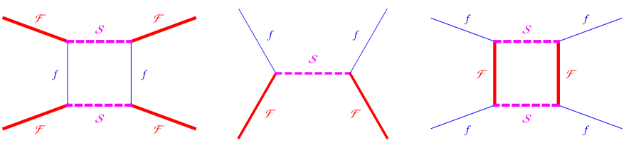
Figure 1: We here denote as $f$ the SM fermions, as ${\cal F}$ the TC-fermions and as ${\cal S}$ the TC-scalars. The diagram on the left contributes to ${\cal F}^{4}$ operators, which become the Higgs potential, given that $H\sim{\cal F}{\cal F}$ (extra TC-penguin diagrams are not shown). The tree-level diagram in the middle leads to ${\cal F}^{2}f^{2}$ operators, which become the SM $ffH$ Yukawa couplings. The diagram on the right contributes to $f^{4}$ operators, which give corrections to flavor physics. Each diagram gets dressed by strong TC interactions.

The technicolor group is indicated by $G_{\rm TC}$, which can be either $\,{\rm SU}(N)$, $\,{\rm SO}(N)$ or $\,{\rm Sp}(N)$ with vectorial techni-fermions and techni-scalars. For historical reasons we will use the technicolor (TC) terminology for the underlying composite dynamics.

We will choose the TC-particle content such that it automatically leads to a custodial symmetry, as well as accidental conservation of baryon and lepton number, like in the SM. Partial compositeness is realized provided that the gauge quantum numbers allow each fundamental SM fermion to have a fundamental Yukawa coupling to at least one pair of TC particles:

$$\hbox{(each SM fermion)}\times\hbox{(some TC scalar)}\times\hbox{(some TC fermion).}$$ (1)

Figure 1 illustrates how these Yukawa couplings lead to SM fermions masses at tree level, as well as to an Higgs potential and to new flavor violations at loop level. TC-fermions and TC-scalars acquire specific patterns of accidental global symmetries, spontaneously broken by the TC dynamics: the Higgs can be identified with a light techni-pion (TC$\pi$) made either of two TC-fermions or of two TC-scalars. We further constrain the SM extensions to avoid sub-Planckian Landau poles and require the TC model to lead to chiral symmetry breaking.

The key to the success is to find a TC gauge group and associated TC-fermions and TC-scalars with appropriate SM quantum numbers. In practice this requires satisfying eq. (1) by finding a minimal ‘square root’ of SM fermions gauge quantum numbers. We will show that it is possible to construct successful composite Higgs theories and associated partially composite sectors. Despite the presence of TC-scalars, the Higgs mass is calculable if $H$ is a pseudo-Goldstone boson made of two TC-fermions.

In section 2 we discuss general issues about the strong dynamics of scalars, which has not been studied outside the special case of supersymmetry. We present the separate pieces that must be combined together in succesfull concrete models, which are presented in section 3 (the eager phenomenologist might want to jump here). In section 4 we compute the resulting Higgs physics. We present our conclusions in section 5.

2 General preliminary considerations

We consider a theory with gauge group $G_{\rm TC}\otimes G_{\rm SM}$ and vectorial TC-fermions and TC-scalars in the fundamental of $G_{\rm TC}$ with UV Lagrangian

$$\mathscr{L}=\mathscr{L}_{\rm SM}^{H=0}+\mathscr{L}_{\rm kin}+\mathscr{L}_{Y}-V\,,$$ (2)

where $\mathscr{L}_{\rm kin}$ contains kinetic, gauge interactions, and possible masses $m_{\cal F}$ and $m_{\cal S}$ for the TC particles.

We use a compact notation for the particle spectrum quantum numbers under the SM gauge group $G_{\rm SM}=\,{\rm SU}(3)_{c}\otimes\,{\rm SU}(2)_{L}\otimes\,{\rm U}(1)_{Y}$ that we exemplify via the SM fermion fields:

$$L=(1,2)_{-1/2},~{}E=(1,1)_{1},~{}Q=(3,2)_{1/6},~{}U=(\bar{3},1)_{-2/3},~{}D=(\bar{3},1)_{1/3},~{}N=(1,1)_{0}\ .$$ (3)

We define as $R^{c}$ the representation conjugated to $R$, e.g. $U^{c}=(3,1)_{2/3}$.

We indicate Weyl TC-fermions by ${\cal F}$ and generically complex TC-scalars by ${\cal S}$. They will decompose under $G_{\rm SM}$ as:

$${\cal F}={\cal F}_{L}\oplus{\cal F}_{E}\oplus{\cal F}_{Q}\oplus{\cal F}_{U}\oplus{\cal F}_{D}\oplus{\cal F}_{N}\oplus\cdots,\qquad{\cal S}={\cal S}_{L}\oplus{\cal S}_{E}\oplus{\cal S}_{Q}\oplus{\cal S}_{U}\oplus{\cal S}_{D}\oplus{\cal S}_{N}\oplus\cdots$$ (4)

with, for example,

$${\cal F}_{L}=(1,2)_{-1/2}\ ,\qquad{\cal S}_{Q}=(3,2)_{1/6}\qquad{\rm under}~{}G_{\rm SM}.$$ (5)

Clearly each ${\cal F}$ and ${\cal S}$ field carries a further gauge index under $G_{\rm TC}$ that we omitted.

In the following we will consider for $G_{\rm TC}$ either $\,{\rm SU}(N)$, $\,{\rm SO}(N)$ or $\,{\rm Sp}(N)$ gauge groups and we will assume TC-fermions and TC-scalars to live in the fundamental of these groups, which minimize the contributions to gauge $\beta$ functions, as needed for successful models. We will consider TC-fermions vector-like with respect to $G_{\rm TC}$ (in the $\,{\rm SU}(N)_{\rm TC}$ case for each TC-fermion ${\cal F}$ in the fundamental there will be also ${\cal F}^{c}$ in the anti-fundamental) and to $G_{\rm SM}$.

2.1 Accidental global symmetries

We now classify the global symmetries of a given TC theory for different choices of $G_{\rm TC}$, once the SM interactions are switched off.

• $G_{\rm TC}=\,{\rm SU}(N)_{\rm TC}$ for $N>2$ has a complex fundamental. The vectorial TC-fermions ${\cal F}$ can be organized in terms of Dirac spinors $\Psi_{{\cal F}}=({\cal F},\bar{\cal F}^{c})^{T}$ and the kinetic term can be written as

  $$\mathscr{L}_{\rm kin}=-\frac{1}{4}{\cal G}_{\mu\nu}^{2}+\overline{\Psi}_{{\cal F}}(i\not{D}-m_{{\cal F}})\Psi_{{\cal F}}+(|D_{\mu}{\cal S}|^{2}-m_{\cal S}^{2}|{\cal S}|^{2})\,,$$ (6)

  where the sum over color and flavor indices is understood. Ignoring the SM gauge interactions, the fermionic kinetic term has a ‘TC flavor’ non-anomalous global symmetry $\,{\rm SU}(N_{F})_{L}\otimes\,{\rm SU}(N_{F})_{R}\otimes\,{\rm U}(1)_{V}$, where $N_{F}$ is the dimension of the SM representation to which ${\cal F}$ belongs to, that for ${\cal F}={\cal F}_{E}\oplus{\cal F}_{L}+\cdots$ is $N_{F}=\dim L+\dim E+\cdots$.

  In the scalar sector, the kinetic term of TC scalars similarly has a $\,{\rm SU}(N_{S})\otimes\,{\rm U}(1)_{S}$ global symmetry where $N_{S}$ counts the number of complex scalars in the fundamental of TC, that for ${\cal S}={\cal S}_{E}\oplus{\cal S}_{L}+\cdots$ is $N_{S}=\dim L+\dim E+\cdots$.

• $G_{\rm TC}=\,{\rm SO}(N)_{\rm TC}$ has a vectorial real representation and therefore Weyl spinors ${\cal F}$ in the fundamental of TC must lie in a real representation of $G_{\rm SM}$. The global symmetry is $\,{\rm SU}(N_{F})$ with $N_{F}$ the dimension of the real SM representation to which ${\cal F}$ belongs to.

  In the scalar sector, we define $N_{S}$ as the number of real copies of $N$: for example $N_{S}=6$ for a TC-scalar in the fundamental 3 of $\,{\rm SU}(3)_{c}$ and $N_{S}=3$ for a TC-scalar in the 3 of $\,{\rm SU}(2)_{L}$. The scalar kinetic term $(D_{\mu}{\cal S}_{i})^{T}(D_{\mu}{\cal S}^{i})$ has accidental global symmetry $\,{\rm SO}(N_{S})\otimes\mathbb{Z}_{2}$.

• $G_{\rm TC}=\,{\rm Sp}(N)_{\rm TC}$ with even $N$ is defined as the group of matrices that leave invariant the antisymmetric tensor $\gamma=\varepsilon\otimes\mathbb{I}_{N/2}$ where $\varepsilon=i\sigma_{2}$ is the 2-dimensional antisymmetric tensor. The fundamental of $\,{\rm Sp}(N)$ is pseudo-real (see appendix A). Again, we consider vectorial TC-fermions ${\cal F}$ constructing vectorial SM representations, with $N_{F}$ Weyl fermions in the fundamental of $\,{\rm Sp}(N)_{\rm TC}$. $N_{F}$ counts the dimension of the real SM representation of ${\cal F}$ and it must be even to avoid the Witten topological anomaly. As for the orthogonal TC gauge group the fermion kinetic term has the non-abelian global symmetry $\,{\rm SU}(N_{F})$.

  In the scalar sector, the kinetic term of $N_{S}$ complex scalars in the $N$ of $\,{\rm Sp}(N)_{\rm TC}$ has accidental global symmetry $\,{\rm Sp}(2N_{S})$, see appendix A. For example, a scalar in the $(3,N)$ of $\,{\rm SU}(3)_{c}\otimes\,{\rm Sp}(N)_{\rm TC}$ has $N_{S}=3$ and global symmetry $\,{\rm Sp}(6)$.

The global symmetries of the kinetic terms are summarized in table 1.

$$\begin{array}[]{|c|c|ccccc|}\hline\cr\hbox{Fields}&\hbox{Gauge}&\lx@intercol\hfil\hbox{Global symmetry of fermions}\hfil\lx@intercol\vrule\lx@intercol&\lx@intercol\hfil\hbox{Global, scalars}\hfil\lx@intercol\vrule\lx@intercol\\ \hline\cr\hline\cr&\,{\rm SU}(N)_{\rm TC}&\,{\rm SU}(N_{F})_{L}&\,{\rm SU}(N_{F})_{R}&\,{\rm U}(1)_{V}&\,{\rm SU}(N_{S})&\,{\rm U}(1)_{S}\\ \hline\cr{\mathcal{F}}&N&N_{F}&1&+1&1&0\\ {\mathcal{F}}^{c}&\bar{N}&1&\bar{N}_{F}&-1&1&0\\ {\mathcal{S}}&N&1&1&0&N_{S}&1\\ \hline\cr\hline\cr&\,{\rm SO}(N)_{\rm TC}&&\,{\rm SU}(N_{F})&&\mathrm{O}(N_{S})&\\ \hline\cr{\mathcal{F}}&N&&N_{F}&&1&\\ {\mathcal{S}}&N&&1&&N_{S}&\\ \hline\cr\hline\cr&\,{\rm Sp}(N)_{\rm TC}&&\,{\rm SU}(N_{F})&&\,{\rm Sp}(2N_{S})&\\ \hline\cr{\mathcal{F}}&N&&N_{F}&&1&\\ {\mathcal{S}}&N&&1&&2N_{S}&\\ \hline\cr\end{array}$$

Table 1: Gauge and local non anomalous symmetries of generic models with gauge group $G_{\rm TC}=\,{\rm SU}(N)_{\rm TC}$ or $\,{\rm SO}(N)_{\rm TC}$ or $\,{\rm Sp}(N)_{\rm TC}$ and $N_{F}$ ($N_{S}$) TC-fermions (TC-scalars) in the $N$ representation; for $\,{\rm SU}(N)_{\rm TC}$ and $\,{\rm Sp}(N)_{\rm TC}$ we count complex scalars, for $\,{\rm SO}(N)_{\rm TC}$ we count real scalars.

Group theory allows to construct renormalizable Yukawa operators of the form of eq. (1). (For $N=3$ Yukawa interactions among 3 TC particles are also possible). These are the operators leading naturally to the partial compositeness scenario. In fact when the techni-force is strong enough it will create the fermionic bound state ${\cal B=FS}$ that already has mass dimension 5/2 at the engineering level. Also, we do not need an extra mechanism or additional force to construct the overall ${f\cal B}$ operator. Furthermore, since any other construction for partial compositeness will have to yield a composite fermion with at most mass dimension 5/2 we expect that at the effective description level it will reduce to our construction. The simplest example is a TC-baryon emerging from an $\,{\rm SU}(3)_{\rm TC}$ gauge theory with fundamental TC-fermions. In this case, at the fundamental level, the TC-baryon will be made by three TC-fermions that can always be represented as a bound state of one TC-fermion and a TC-scalar with the quantum numbers of di-techniquarks. It is a simple matter to show that this intermediate dynamical description can be generalized to the case in which a TC-baryon is made by TC-fermions in multiple TC representations. Of course, in the purely fermionic case, one must argue for the existence of near conformal non-supersymmetric quantum field theories yielding baryon operators with unplausibily large [11] anomalous dimensions.

2.2 Quartic couplings among TC-scalars

TC-scalars develop self-interactions generated by RGE effects via, for example, their gauge interactions. These effects are encoded in $\beta$ functions $\beta_{\lambda}=d\lambda/d\ln E$ which at one loop assume the generic form $(4\pi)^{2}\beta_{\lambda}\sim+\lambda^{2}+g^{4}_{\rm TC}-\lambda g^{2}_{\rm TC}$. Here we indicated the generic scalar self-couplings by $\lambda$ and the TC gauge coupling with $g_{\rm TC}$. Running down to low energy, when the TC gauge coupling start becoming strong, quartics become of order $\pm g^{2}_{\rm TC}$, where the sign depends on the specific model. This means that, if quartics remain positive up to the confinement scale, they also contribute to the nonperturbative dynamics of the theory. In this case, a simplifying assumption is to use flavor universal quartics in order not to spoil the symmetries of the scalar sector listed in Table 1. If, on the other hand, quartics become negative at some energy scale, the Coleman-Weinberg mechanism can take place.

To estimate the effects on the quartic self-couplings we consider $N_{S}$ scalars in the fundamental of $\,{\rm SU}(N)_{\rm TC}$, such that TC-scalars ${\cal S}$ form a complex $N\times N_{S}$ matrix. At very high energies, because the couplings are assumed to be small, we can ignore masses and cubic interactions, and we write the following quartic potential including only the $\,{\rm SU}(N_{S})$ flavor-symmetric operators

$$V=\lambda_{\cal S}\,{\rm Tr}({\cal S}{\cal S}^{\dagger})^{2}+\lambda^{\prime}_{\cal S}\,{\rm Tr}({\cal S}{\cal S}^{\dagger}{\cal S}{\cal S}^{\dagger}).$$ (7)

Such potential is definite positive for $\lambda_{{\cal S}}+r\lambda^{\prime}_{{\cal S}}>0$ where $r=\,{\rm Tr}({\cal S}{\cal S}^{\dagger}{\cal S}{\cal S}^{\dagger})/\,{\rm Tr}({\cal S}{\cal S}^{\dagger})^{2}$ ranges between $1/\min(N,N_{S})$ and $1$. The relevant one-loop RGEs are

$$\halign to=0.0pt{\@eqnsel\hskip\@centering$\displaystyle{#}$&\global\@eqcnt\@ne\hskip 2\arraycolsep\hfil${#}$\hfil& \global\@eqcnt\tw@\hskip 2\arraycolsep$\displaystyle{#}$\hfil&\llap{#}\cr 0.0pt plus 1000.0pt$\displaystyle{(4\pi)^{2} \beta_{g_{\rm TC}}&10.0pt\hfil${=&10.0pt$\displaystyle{bg_{\rm TC}^{3}\\ (4\pi)^{2} \beta_{\lambda_{\cal S}} &\hbox to0.0pt{\hss=&4(NN_{S}+4)\lambda_{\cal S}^{2}+12\lambda_{\cal S}^{\prime 2}+\\&&+\lambda_{\cal S}\bigg{[}8(N+N_{S})\lambda_{\cal S}^{\prime}-\frac{6(N^{2}-1)}{N}g^{2}_{\rm TC}\bigg{]}+\frac{3(N^{2}+2)}{4N^{2}}g^{4}_{\rm TC},\\(4\pi)^{2}\beta_{\lambda_{\cal S}^{\prime}}&=&4(N+N_{S})\lambda_{\cal S}^{\prime 2}+\lambda_{\cal S}^{\prime}\bigg{[}24\lambda_{\cal S}-\frac{6(N^{2}-1)}{N}g^{2}_{\rm TC}\bigg{]}+\frac{3(N^{2}-4)}{4N}g^{4}_{\rm TC}.&(8)\cr}}}}}$$

The left panel of fig. 2 shows a sample numerical solution in the model that will be proposed in section 3.1: quartic couplings can remain numerically small up to the Planck scale. The right panel shows the pseudo-fixed point structure of a different model that admits two pseudo-fixed points (namely, $\lambda/g^{2}_{\rm TC}$ flow to constant values) with positive values of the quartics, which can flow from one point to the other. The pseudo-fixed-point conditions can be solved analytically in general [26] and acquire a simple form in the large $N$ limit, where the equations for the two quartics basically decouple, showing that pseudo-fixed points $\lambda\sim g^{2}_{\rm TC}\sim 1/N$ exist for $N_{S}<2N+b+b^{2}/12N$.

      

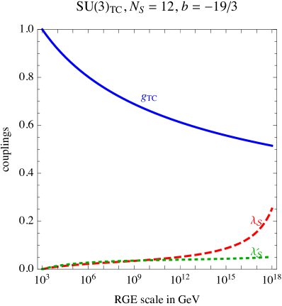
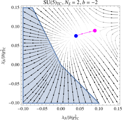
Figure 2: Left: numerical solution to the RGE in the model of section 3.1. Right: pseudo-fixed point structure of a model with 2 pseudo-fixed points (shown as dots); the scalar potential becomes unstable when quartics flow into the shaded region.

The overall conclusion is that techni-quartic interactions can be well defined till the Planck scale (either with or without interacting pseudo-fixed points) and furthermore that there are theories in which the low energy physics is driven by the techni-gauge interactions becoming strong.

$$\begin{array}[]{c|cc}\hbox{Gauge group}&\hbox{Fermion bilinear condensate}&\hbox{Intact scalar symmetries}\\ \hline\cr\,{\rm SU}(N)_{\rm TC}&\,{\rm SU}(N_{F})_{L}\otimes\,{\rm SU}(N_{F})_{R}\to\,{\rm SU}(N_{F})&\,{\rm U}(N_{S})\\ \,{\rm SO}(N)_{\rm TC}&\,{\rm SU}(N_{F})\to\,{\rm SO}(N_{F})&\mathrm{O}(N_{S})\\ \,{\rm Sp}(N)_{\rm TC}&\,{\rm SU}(N_{F})\to\,{\rm Sp}(N_{F})&\,{\rm Sp}(2N_{S})\end{array}$$

Table 2: Pattern of chiral symmetry breaking induced by fermion condensates ${\cal F}{\cal F}^{c}$ for $\,{\rm SU}(N)_{\rm TC}$ and ${\cal F}{\cal F}$ for $\,{\rm SO}(N)_{\rm TC}$ and $\,{\rm Sp}(N)_{\rm TC}$. An explicit positive squared mass term for the scalars ensures that the scalar symmetries remain intact.

2.3 Dynamical symmetry breaking

The analysis above allows us to assume the new strong interaction to be asymptotically free and further require that the force is sufficiently strong to confine the fundamental degrees of freedom into techni-hadrons at a scale $\Lambda_{\rm TC}\,\raise 1.29167pt\hbox{$>$\kern-7.5pt\lower 4.30554pt\hbox{$\sim$}}\,$ TeV. Asymptotic freedom is realized when the first order coefficient of the gauge $\beta$ function is negative. We fill further impose stronger conditions under which it is reasonable to expect that the underlying dynamics does not display large distance conformality [27, 28]. We will limit here to investigate condensation phenomena induced by the techni-strong force that leave intact the TC gauge interactions.

Fermion condensates

We start by reviewing the pattern of chiral symmetry breaking expected to occur when fermion-bilinear Lorentz preserving condensates form.

In asymptotically free theories with only vector-like fermions one can show [30] that the associated condensates preserve the gauge group (e.g.  only gauge-singlets $\langle\bar{\psi}_{L}\psi_{R}\rangle$ can form in $\,{\rm SU}(N)_{\rm TC}$ theories). Furthermore, it is often argued that non-vanishing fermion condensates orient in such a way to preserve as much as possible of the original global symmetry provided the massless spectrum is compatible with the t’Hooft anomaly conditions and other relevant constraints. The pattern of symmetry breaking implied by such arguments is summarized in table 2. This means that for $G_{\rm TC}=\,{\rm SU}(N)_{\rm TC}$ the TC$\pi$ are made of ${\cal F}{\cal F}^{c}$ states (with ${\cal F}$ a Dirac fermion) and for $\,{\rm SO}(N)_{\rm TC}$ and $\,{\rm Sp}(N)_{\rm TC}$ are made of ${\cal F}{\cal F}$ (with ${\cal F}$ a Weyl fermion).

Scalar condensates

In the presence of scalars, various dynamical phases can occur. A detailed dynamical study goes beyond the scope of this work, where we just describe the possible patterns of chiral symmetry breaking in the scalar sector stemming from scalar bilinears. The fact that both scalar and fermion bilinears form is partially supported by the intuition gained via the naive most attractive channels approach (MAC) [31] that here we take merely as guidance. Furthermore, because of the anti-commutative nature of composite operators $\bar{{\cal F}}{\cal S}$, they cannot acquire a vacuum expectation value and therefore Lorentz invariance is preserved.

An interesting class of models is the one in which the fermions condense and break their global symmetries while the scalars do not break neither their global symmetries nor the gauge interactions. This can be achieved by endowing the scalars with a positive mass squared respecting the gauge and scalar global symmetries. In this case the symmetries of the theory are presented in table 2. For the scalars to still be actively participating in the TC dynamics we require the explicit common scalar masses to be of the order or smaller than the TC dynamical scale, $m_{\cal S}\,\raise 1.29167pt\hbox{$<$\kern-7.5pt\lower 4.30554pt\hbox{$\sim$}}\,\Lambda_{\rm TC}$.

Depending on the mass squared term and the strong dynamics one could also have partial spontaneous symmetry breaking of some of their global symmetries and Higgsing of gauge interactions. One of these possibilities will be summarized in table 5. Alternatively, scalars could break their global symmetries while still leaving confinement intact. Scalar condensates proportional to the unity matrix in flavor space do not explicitly break the global accidental symmetry in the scalar sector. This breaking arises if scalars develop flavor non-universal condensates. For example, TC-scalars with the quantum numbers of $L$ and $N$ and a $\langle{\cal S}_{N}{\cal S}^{*}_{N}\rangle$ condensate would give rise to the pattern of global symmetry breaking $\,{\rm U}(3)\to\,{\rm U}(2)$ leading to a Goldstone boson ${\cal S}_{L}{\cal S}_{N}^{*}$ with the quantum numbers of a Higgs doublet plus a singlet.

Naive conformal window

If the number of matter fields of the theory is sufficiently large, and in absence of a Higgsing phenomenon, the TC dynamics can develop an infrared interacting fixed point. In this scenario no dynamical scale forms at low energies, before coupling the theory to the SM. Since we want the fermions to condense, we must lie outside the conformal window. We provide a crude estimate of the ‘safe’ region of number of fermions and scalars as a function of the number of TC ($N$) where we expect dynamical condensation to occur.

The one loop $\beta$ function for $g_{\rm TC}$ is:

$$\beta_{\rm TC}^{(1)}=\frac{g_{\rm TC}^{3}}{(4\pi)^{2}}\left[-\frac{11}{3}C_{2}({\rm Adj})+\frac{2}{3}T(F)m(F)+\frac{1}{3}T(S)m(S)\right]\,,$$ (9)

where $F$ and $S$ denote the Weyl fermion and complex scalar representations respectively and $m(F)$, $m(S)$ their multiplicity. In the $\,{\rm SU}(N)_{\rm TC}$ case $m(F)=2N_{F}$ and $m(S)=N_{S}$, for $\,{\rm SO}(N)_{\rm TC}$ we have $m(F)=N_{F}$ and $m(S)=N_{S}/2$, while for $\,{\rm Sp}(N)_{\rm TC}$, $m(F)=N_{F}$ and $m(S)=N_{S}$ with $N_{F}$ and $N_{S}$ defined in section 2.1 for each choice of $G_{\rm TC}$.

We simply assume that condensates are formed if the first coefficient of the full beta function $\beta^{(1)}_{\rm TC}$, in modulus, is larger than the third of the modulus of the first coefficient of the gauge beta function, i.e. $\beta_{\rm TC}^{(1)}\,\raise 1.29167pt\hbox{$<$\kern-7.5pt\lower 4.30554pt\hbox{$\sim$}}\,\frac{1}{3}\beta^{(1)}_{\rm TC}|_{\rm gauge}$. This is intuitively reasonable since matter screens the confining gauge interactions and the resulting naive condition is roughly compatible with earlier estimates [27, 28, 32, 33, 34]. Considering TC-fermions and TC-scalars in the fundamental of the gauge group we obtain the following conditions:

$$\begin{array}[]{cccc}G&C_{2}({\rm Adj})&T(F)=T(S)&\hbox{Condensates form if}\\ \,{\rm SU}(N)_{\rm TC}&N&\frac{1}{2}&\displaystyle N\,\raise 1.29167pt\hbox{$>$\kern-7.5pt\lower 4.30554pt\hbox{$\sim$}}\,\frac{3(4N_{F}+N_{S})}{44}\\ \,{\rm SO}(N)_{\rm TC}&N-2&1&\displaystyle N\,\raise 1.29167pt\hbox{$>$\kern-7.5pt\lower 4.30554pt\hbox{$\sim$}}\,\frac{3(4N_{F}+N_{S})}{44}+2\\ \,{\rm Sp}(N)_{\rm TC}&\frac{1}{2}(N+2)&\frac{1}{2}&\displaystyle N\,\raise 1.29167pt\hbox{$>$\kern-7.5pt\lower 4.30554pt\hbox{$\sim$}}\,\frac{3(2N_{F}+N_{S})}{22}-2\\ \end{array}$$ (10)

To clarify the counting of fermions and scalars, we consider for example a TC-fermion and a TC-scalar in the fundamental of the TC group and in the $2_{-1/2}$ of $\,{\rm SU}(2)_{L}\otimes\,{\rm U}(1)_{Y}$, if the TC group is $\,{\rm SU}(N)_{\rm TC}$ we have $N_{F}=N_{S}=2$, if it is $\,{\rm SO}(N)_{\rm TC}$ we have $N_{F}=N_{S}=4$ and if it is $\,{\rm Sp}(N)_{\rm TC}$ we have $N_{F}=2N_{S}=4$.

2.4 Custodial symmetry

The $T$ parameter agrees with SM predictions and gives a strong bound on the $|H^{\dagger}D_{\mu}H|^{2}$ effective operator which can arise in models where $H$ is composite. The typical correction is of order $\hat{T}\sim v^{2}/f_{\rm TC}^{2}$ such that the experimental bound $|\hat{T}|\,\raise 1.29167pt\hbox{$<$\kern-7.5pt\lower 4.30554pt\hbox{$\sim$}}\,2\times 10^{-3}$ would imply $f_{\rm TC}\,\raise 1.29167pt\hbox{$>$\kern-7.5pt\lower 4.30554pt\hbox{$\sim$}}\,5\,{\rm TeV}$ and a correspondingly large unnatural correction to the Higgs mass. This unseen deviation from the SM is much suppressed if the Higgs sector respects a ‘custodial’ symmetry $\,{\rm SU}(2)_{L}\otimes\,{\rm SU}(2)_{R}\to\,{\rm SU}(2)_{c}$ [35]. In fundamental models such symmetry must be a consequence of the TC-fermion content, arising as an accidental global symmetry. Below we list the simplest possibilities that lead to a custodial symmetry. Considering first the case in which the Higgs is a TC$\pi$ made of two TC-fermions:

1. The most minimal model is obtained considering $G_{\rm TC}=\,{\rm Sp}(N)$ with TC-fermions ${\cal F}=2_{0}\oplus 1_{1/2}\oplus 1_{-1/2}$ under $\,{\rm SU}(2)_{L}\otimes\,{\rm U}(1)_{Y}$. If their mass differences are much smaller than $\Lambda_{\rm TC}$, the TC dynamics respects a global symmetry $\,{\rm SU}(4)$ broken to $\,{\rm Sp}(4)$, leading to TC$\pi$ in a $(2,2)\oplus(1,1)$ of $\,{\rm SU}(2)_{L}\otimes\,{\rm SU}(2)_{R}$, among which we can identify the composite Higgs doublet. In general, whenever there is one Higgs doublet, the custodial symmetry is ensured when the unbroken global symmetry group contains a subgroup $\,{\rm SO}(4)\supset\,{\rm SU}(2)_{L}\otimes\,{\rm SU}(2)_{R}$. Lattice simulations [36] find that the pattern of chiral symmetry breaking envisioned above is indeed achieved for the minimal $\,{\rm SU}(2)\sim\,{\rm Sp}(2)$ case.

2. Another minimal possibility arises from $\,{\rm SO}(N)_{\rm TC}$ with TC-fermions ${\cal F}={\cal F}_{L}\oplus{\cal F}_{L^{c}}\oplus{\cal F}_{N}$. If their mass differences are much smaller than $\Lambda_{\rm TC}$, dynamics respects a global symmetry $\,{\rm SU}(5)$ spontaneously broken to $\,{\rm SO}(5)$, delivering TC$\pi$ in the $(1,1)\oplus(2,2)\oplus(3,3)$ of $\,{\rm SU}(2)_{L}\otimes\,{\rm SU}(2)_{R}$. One must check that the extra scalars, such as the triplet in ${\cal F}_{L}{\cal F}_{L^{c}}$, acquire positive squared masses and have no vev.

3. Finally, $\,{\rm SU}(N)_{\rm TC}$ with $N\geq 3$ and TC-fermions ${\cal F}={\cal F}_{L}\oplus{\cal F}_{E^{c}}\oplus{\cal F}_{N}$ respects a global symmetry $\,{\rm SU}(4)_{L}\otimes\,{\rm SU}(4)_{R}$ spontaneously broken to $\,{\rm SU}(4)_{V}$. If the mass difference between ${\cal F}_{E^{c}}$, ${\cal F}_{N}$ is much smaller than $\Lambda_{\rm TC}$, TC-strong dynamics respects a global custodial $\,{\rm SU}(2)_{L}\otimes\,{\rm SU}(2)_{R}$ symmetry, under which the TC$\pi$ in the adjoint of $\,{\rm SU}(4)_{V}$ transform as $2\times(2,2)\oplus(1,1)\oplus(3,1)\oplus(1,3)$. Unlike in the previous cases, one has a complex bidoublet of Higgses: in the presence of two Higgs doublets, a generic minimum of the potential breaks the electro-weak and the custodial symmetry. The vacuum expectation values of the two Higgses must be aligned. A generic potential can have appropriate minima [37]; however special potentials (such as those arising for TC$\pi$) can need an extra discrete symmetry in order to obtain the desired alignement [38]. One must check that the extra scalars, such as the triplet in ${\cal F}_{L}{\cal F}^{c}_{L}$, acquire positive squared masses, and have no vacuum expectation values.

We next consider the case where the Higgs is a TC$\pi$ made of two TC-scalars, recalling that they can have the accidental global symmetry listed in table 2, and that its breaking pattern is model dependent. We assume that scalar condensates preserve $G_{\rm TC}$ and break the global symmetry as follows:

• $\,{\rm SU}(N)_{\rm TC}$ with TC-scalars ${\cal S}={\cal S}_{L}\oplus{\cal S}_{E^{c}}\oplus{\cal S}_{N}$ respects a global $\,{\rm SU}(4)$ symmetry. A $G_{\rm SM}$-preserving condensate $\langle{\cal S}^{*}{\cal S}\rangle=f^{2}{\mathbb{I}}+f^{\prime 2}\,{\rm diag}(0,0,1,1)$ would break it into $\,{\rm SU}(2)_{L}\otimes\,{\rm SU}(2)_{R}$, leading to two custodially protected Higgs doublets. The TC$\pi$ decompose as $2\times(2,2)\oplus(1,1)$ under the $\,{\rm SU}(2)_{L}\otimes\,{\rm SU}(2)_{R}$ unbroken symmetry.

• $\,{\rm SO}(N)_{\rm TC}$ with TC-scalars ${\cal S}={\cal S}_{L}\oplus{\cal S}_{N}$ respects a global $\,{\rm SO}(5)$ symmetry. The most generic $G_{\rm SM}$-preserving condensate $\langle{\cal S}{\cal S}\rangle=f^{2}{\mathbb{I}}+f^{\prime 2}\,{\rm diag}(0,0,0,0,1)$ would break it into $\,{\rm SO}(4)$, leading to one custodially protected Higgs doublet.

• $\,{\rm Sp}(N)_{\rm TC}$ with TC-scalars ${\cal S}={\cal S}_{L}\oplus{\cal S}_{N}$ respects a global $\,{\rm Sp}(6)$ symmetry. The $G_{\rm SM}$-preserving condensate $\langle{\cal S}{\cal S}\rangle=\varepsilon\otimes\,{\rm diag}(f^{2},f^{2},f^{2}+f^{\prime 2})$ breaks $\,{\rm Sp}(6)\to\,{\rm Sp}(4)\otimes\,{\rm Sp}(2)$, leading to 8 TC$\pi$ that decompose under $\,{\rm SU}(2)_{L}\otimes\,{\rm SU}(2)_{R}$ as $2\times(2,2)$, giving two custodially protected Higgs doublets.

Custodial symmetry for $Z\to b\bar{b}$

In order to reproduce the large top Yukawa coupling, the 3rd-generation $Q=(t_{L},b_{L})$ must be significantly mixed with composite fermions ${\cal B}$. This can give gauge interactions that deviate from those of an elementary fermion. Thereby a correction of order $\delta g_{b_{L}}\sim v^{2}/\Lambda_{\rm TC}^{2}$ to the $Zb_{L}\bar{b}_{L}$ coupling would imply $\Lambda_{\rm TC}\,\raise 1.29167pt\hbox{$>$\kern-7.5pt\lower 4.30554pt\hbox{$\sim$}}\,5\,{\rm TeV}$. This bound is less severe than the one from the $T$ parameter, but it is serious enough that various authors have discussed how to alleviate it via effective field theories with extra custodial symmetries  [39]. One such example needs a left-right symmetry that exchanges $\,{\rm SU}(2)_{L}$ with $\,{\rm SU}(2)_{R}$ and that $b_{L}$ respects the condition $T_{L}=T_{R}$ and $T^{3}_{L}=T^{3}_{R}$ under the custodial group [39]. This can be realized if the composite spectrum in the top sector is $LR$-symmetric and if the SM quark doublet $Q=(t_{L},b_{L})$ couples with a composite quark in a $(2,2)_{2/3}$ of $\,{\rm SU}(2)_{L}\otimes\,{\rm SU}(2)_{R}\otimes\,{\rm U}(1)_{X}$ where $Y=T_{R}^{3}+X$. The embedding of $b_{L}$ into such a representation satisfies the condition above.

In the fundamental theory, this protection mechanism occurs automatically in the $\,{\rm SO}(N)_{\rm TC}$ model described above, with TC-fermions ${\cal F}={\cal F}_{L}\oplus{\cal F}_{L^{c}}\oplus{\cal F}_{N}$. In fact, if the mass difference between ${\cal F}_{L}$ and ${\cal F}_{L^{c}}$ is much smaller than $\Lambda_{\rm TC}$ they form a left-right-symmetric bidoublet. Adding a TC-scalar ${\cal S}_{U^{c}}$ allows to couple the SM quarks $Q$ and $U$ to the TC-particles, obtaining the top Yukawa couplings. Then, the fermionic bound states ${\cal B}={\cal F}{\cal S}$ contain an accidentally degenerate pair of composite fermions ${\cal S}_{U^{c}}{\cal F}_{L}=(3,2)_{1/6}$ and ${\cal S}_{U^{c}}{\cal F}_{L^{c}}=(3,2)_{7/6}$, where we showed the SM gauge quantum numbers. By mixing with them, $Q$ keeps its SM value of the $Zb\bar{b}$ coupling, up to higher order corrections. A model will be discussed in section 3.5. In the $\,{\rm SU}(N)_{\rm TC}$ and $\,{\rm Sp}(N)_{\rm TC}$ cases such a mechanism would require a more involved construction.

3 Successful models

Having discussed separately the main ingredients, we now study if concrete models exist that realize simultaneously all the 4 following conditions:

• The new strong gauge interaction is asymptotically free and generates condensates. For a given content of TC-particles, this implies an approximated lower bound on $N$, see eq. (10).

• All couplings can be extrapolated up to the Planck scale without hitting Landau poles. For the SM gauge couplings this implies that their one-loop $\beta$ function coefficients $b_{i}$ defined by $d\alpha_{i}^{-1}/d\log E=-b_{i}/2\pi+\cdots$ must satisfy the conditions

  $$b_{3}\lesssim 1.9\,,\qquad b_{2}\lesssim 5.3\,,\qquad b_{1}\lesssim 10$$ (11)

  having assumed $\Lambda_{\rm TC}\sim\,{\rm TeV}$ and written $b_{1}$ in $\,{\rm SU}(5)_{\rm GUT}$ normalization (equivalently $b_{Y}=\frac{5}{3}b_{1}\lesssim 16.6$). For a given TC-particle content, these conditions imply an upper bound on $N$.

  The above two requirements are compatible if the TC-particle content is small enough. However, the third condition requires a large enough TC-particle content.

• Each generation of SM fermion $L,D,U,Q,E$ must acquire mass. In effective scenarios, one requires that each SM fermion mixes with a composite state; in our models this translates into Yukawa couplings involving a SM fermion, a TC-scalar and a TC-fermion. But this is not enough: it can still happen that some masses are either forbidden for symmetry reasons and/or that operators that break baryon and lepton number are generated.

The above conditions eliminate the most naive models and require us to devise an economical enough set of TC-particles with the same accidental $\,{\rm U}(1)_{B,L}$ symmetries of the SM. Quarks with equal baryon number and leptons with equal lepton number can be combined in right-handed doublets $Q_{R}=\{U,D\}$ and $L_{R}=\{E,N\}$, where $N$ is an optional right-handed neutrino. The Yukawa couplings must have the generic form

$$\mathscr{L}_{Y}\sim(Q{\cal F}{\cal S}^{*}_{q}+Q_{R}{\cal F}^{c}{\cal S}_{q})+(L{\cal F}{\cal S}_{\ell}^{*}+L_{R}{\cal F}^{c}{\cal S}_{\ell})$$ (12)

such that the (so far unspecified) TC-particles ${\cal F},{\cal S}_{q,\ell}$ mediate all SM Yukawa couplings. This can be more easily seen in the artificial limit where the TC-scalars ${\cal S}_{\ell,q}$ are so heavy that they can be integrated out at tree level as in fig. 1, giving rise to 4-fermions operators $LL_{R}{\cal F}{\cal F}^{c}+QQ_{R}{\cal F}{\cal F}^{c}$. A similar structure arises if TC-scalars are below the confinement scale. The TC-fermion bilinears necessarily have the quantum numbers of a Higgs doublet, and do not contain any lepto-quark.

The fact that an $\,{\rm SU}(2)_{R}$ structure automatically emerges is beneficial for the last condition.

• The model must be compatible with experimental bounds. LHC bounds force the new particles to be heavier than about $\Lambda_{\rm TC}\,\raise 1.29167pt\hbox{$>$\kern-7.5pt\lower 4.30554pt\hbox{$\sim$}}\,1\,{\rm TeV}$. Precision data (mostly the $T$ parameter and $Zb_{L}\bar{b}_{L}$) imply the stronger bound $\Lambda_{\rm TC}\,\raise 1.29167pt\hbox{$>$\kern-7.5pt\lower 4.30554pt\hbox{$\sim$}}\,5\,{\rm TeV}$, corresponding to a large fine-tuning ${\rm FT}\,\raise 1.29167pt\hbox{$>$\kern-7.5pt\lower 4.30554pt\hbox{$\sim$}}\,100$ in the Higgs mass. One can follow different strategies, and it is not clear which one is preferable:

  • Accept a large fine-tuning.

  • Build ad-hoc models aiming at suppressing the unnaturally large quantum corrections to the Higgs mass.

  • Conceive models able to suppress corrections to $T$ and $Zb_{L}\bar{b}_{L}$, such that $\Lambda_{\rm TC}\,\raise 1.29167pt\hbox{$>$\kern-7.5pt\lower 4.30554pt\hbox{$\sim$}}\,1\,{\rm TeV}$ corresponding to ${\rm FT}\,\raise 1.29167pt\hbox{$>$\kern-7.5pt\lower 4.30554pt\hbox{$\sim$}}\,10$, becomes allowed. This can be realized through custodial symmetries that typically need a special TC-particle content.

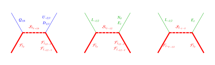
Figure 3: Most general ‘economical’ choice of quantum numbers. The pedices in every field denote the hypercharge and $Y$ is a free constant. 3 denotes a color triplet, 2 a weak doublet and 1 a singlet. Thick lines denote TC-particles; the presence of techni-strong interaction among them is understood.

Figure 3 shows the most general ‘economical’ choice of quantum numbers: in the left diagram we assume that $Q$ couples to a TC-fermion weak doublet ${\cal F}_{2}$ (with generic hypercharge $Y$) and to a TC-scalar color triplet ${\cal S}_{3}$. Then $U$ and $D$ must couple to ${\cal S}_{3}$ and to TC-fermion singlets ${\cal F}_{1}$. In the middle diagram, we next assume that $L$ couples to the same ${\cal F}_{2}$ and to a new TC-scalar singlet ${\cal S}_{1}$; then $E$ and $N$ have hypercharges such that they can couple to the ${\cal F}_{1}$ singlets previously introduced. If $Y=\pm 1/2$, all TC-particles lie in $\,{\rm SU}(5)_{\rm GUT}$ fragments, giving rise to the models described in sections 3.1 and 3.2. The minimal choice $Y=0$ gives the model in section 3.3.

Alternatively, a less minimal model is obtained mediating lepton masses as described in the right diagram (rather than as in the middle diagram): $E$ is coupled to ${\cal F}_{2}$ through a scalar doublet ${\cal S}_{2}$; then $L$ can be coupled to one of the TC-fermion singlets ${\cal F}_{1}$. Right-handed neutrinos $N$ remain uncoupled. The model is described in section 3.4 for $Y=-1/2$.

3.1 Model with $\,{\rm SU}(5)_{\rm GUT}$ fragments and $Y=-1/2$

Referring to the first two diagrams of fig. 3, the choice $Y=-1/2$ corresponds to the TC-particle content

$$N_{g_{F}}\times({\cal F}_{L}\oplus{\cal F}_{E^{c}}\oplus{\cal F}_{N})\oplus N_{g_{S}}\times({\cal S}_{E^{c}}\oplus{\cal S}_{D^{c}}).$$ (13)

For extra clarity, table 3 lists the gauge quantum numbers of the TC-particles. For $G_{\rm TC}=\,{\rm SU}(N)_{\rm TC}$ the most generic Yukawa couplings are

$$\mathscr{L}_{Y}=y_{L}~{}L{\cal F}_{L}{\cal S}_{E^{c}}^{*}+y_{E}~{}E{\cal F}_{N}^{c}{\cal S}_{E^{c}}+(y_{D}~{}D{\cal F}_{N}^{c}+y_{U}~{}U{\cal F}_{E^{c}}^{c}){\cal S}_{D^{c}}+y_{Q}~{}Q{\cal F}_{L}{\cal S}_{D^{c}}^{*}+\hbox{h.c.}$$ (14)

The scalar interactions are

$$\lambda_{E}|S_{E^{c}}|^{4}+\lambda_{ED}|S_{E^{c}}|^{2}\,{\rm Tr}({\cal S}_{D^{c}}{\cal S}_{D^{c}}^{\dagger})+\lambda_{D}\,{\rm Tr}({\cal S}_{D^{c}}{\cal S}_{D^{c}}^{\dagger})^{2}+\lambda^{\prime}_{D}\,{\rm Tr}({\cal S}_{D^{c}}{\cal S}_{D^{c}}^{\dagger}{\cal S}_{D^{c}}{\cal S}_{D^{c}}^{\dagger}).$$ (15)

The renormalizable interactions conserve 5 accidental U(1) global symmetries. First, an anomaly-free TC-baryon number, with charges equal to $+1$ ($-1$) for TC-particles in the $N$ ($\bar{N}$), and to 0 for SM particles. Next, baryon and lepton-number, under which the TC-fermions are neutral and the TC-scalars compensate for the charge of the SM fermions. Finally, two extra U(1) restrict the interactions among SM particles and TC particles. No extra Yukawa couplings nor cubic scalar couplings are allowed for $N=3$.

Analogous Yukawa couplings can be written in the $\,{\rm SO}(N)_{\rm TC}$ ($\,{\rm Sp}(N)_{\rm TC}$) case, with the only difference that the fundamental is a real (pseudo-real) representation, such that one can identify ${\cal F}_{N}={\cal F}_{N}^{c}$ breaking TC-baryon number. For $\,{\rm Sp}(N)_{\rm TC}$ two copies of the ${\cal F}_{N}$ singlet must be considered in order to avoid topological anomalies. The one-loop coefficient of the TC gauge $\beta$ function is

$$b_{\rm TC}=\left\{\begin{array}[]{ll}-\frac{11}{3}N+\frac{2}{3}(4N_{g_{F}}+N_{g_{S}})&{\rm for}\,\,{\rm SU}(N)_{\rm TC}\,,\\ -\frac{11}{3}(N-2)+\frac{2}{3}(7N_{g_{F}}+2N_{g_{S}})&{\rm for}\,\,{\rm SO}(N)_{\rm TC}\,,\\ -\frac{11}{6}(N+2)+\frac{2}{3}(4N_{g_{F}}+N_{g_{S}})&{\rm for}\,\,{\rm Sp}(N)_{\rm TC}\,.\end{array}\right.$$ (16)

We verified that the two-loop term is subdominant for $g_{\rm TC}\,\raise 1.29167pt\hbox{$<$\kern-7.5pt\lower 4.30554pt\hbox{$\sim$}}\,4\pi$. In all cases the one loop coefficients of the SM gauge $\beta$ functions are

$$b_{3}=-7+\frac{N}{6}N_{g_{S}},\qquad b_{2}=-\frac{10}{3}+\frac{2N}{3}N_{g_{F}}\,,\qquad b_{1}=4+\frac{6}{5}NN_{g_{F}}+\frac{4}{15}NN_{g_{S}}.$$ (17)

We assume $N_{g_{F}}=1$, $N_{g_{S}}=3$, which is the most economic choice that allow to write Yukawa couplings for all the 3 generations of SM fermions and to satisfy the conditions on the $\beta$ functions. All gauge $\beta$ functions lie in the allowed range for $1.9\,\raise 1.29167pt\hbox{$<$\kern-7.5pt\lower 4.30554pt\hbox{$\sim$}}\,N<3.0$ in the $\,{\rm SU}(N)_{\rm TC}$ case and for $1.8\,\raise 1.29167pt\hbox{$<$\kern-7.5pt\lower 4.30554pt\hbox{$\sim$}}\,N<3.0$ in the $\,{\rm Sp}(N)_{\rm TC}$ case (for $N=2$ one has $\,{\rm SU}(2)=\,{\rm Sp}(2)$). No solution is found for $\,{\rm SO}(N)_{\rm TC}$.

$$\begin{array}[]{|ccc|cccc|}\hline\cr\hbox{name}&\hbox{spin}&\hbox{generations}&\,{\rm SU}(3)_{c}&\,{\rm SU}(2)_{L}&\,{\rm U}(1)_{Y}&G_{\rm TC}\\ \hline\cr{\cal F}_{N}&1/2&N_{g_{F}}&1&1&0&N\\ {\cal F}_{N}^{c}&1/2&N_{g_{F}}&1&1&0&\bar{N}\\ {\cal F}_{L}&1/2&N_{g_{F}}&1&2&-1/2&N\\ {\cal F}_{L}^{c}&1/2&N_{g_{F}}&1&2&+1/2&\bar{N}\\ {\cal F}_{E^{c}}&1/2&N_{g_{F}}&1&1&-1&N\\ {\cal F}_{E^{c}}^{c}&1/2&N_{g_{F}}&1&1&+1&\bar{N}\\ \hline\cr{\cal S}_{E^{c}}&0&N_{g_{S}}&1&1&-1&N\\ {\cal S}_{D^{c}}&0&N_{g_{S}}&3&1&-1/3&N\\ \hline\cr\end{array}$$

Table 3: Explicit field content of the model of section 3.1 in the case of $G_{\rm TC}=\,{\rm SU}(N)_{\rm TC}$.

Table 2 gives the global symmetry breaking pattern in the fermionic sector: $\,{\rm SU}(8)\to\,{\rm Sp}(8)$ for $\,{\rm Sp}(N)_{\rm TC}$ and $\,{\rm SU}(4)_{L}\otimes\,{\rm SU}(4)_{R}\to\,{\rm SU}(4)_{V}$ for $\,{\rm SU}(N)_{\rm TC}$. The latter possibility corresponds to the minimal one that can realize a custodial symmetry as described in point 2 of section 2.4: the chiral symmetry breaking produces 15 light TC$\pi$ in the adjoint of $\,{\rm SU}(4)_{V}$, that decomposes as

$$\hbox{TC}\pi=2\times(1,1)_{0}\oplus(1,3)_{0}\oplus[(1,1)_{1}\oplus 2\times(1,2)_{-1/2}+\hbox{h.c.}]\qquad\hbox{under $G_{\rm SM}$.}$$ (18)

All TC$\pi$ are unstable. Among these TC$\pi$ we can identify two Higgs doublets that can be embedded in a complex bidoublet of the unbroken custodial symmetry $\,{\rm SU}(2)_{L}\otimes\,{\rm SU}(2)_{R}$. As said above, in the presence of two Higgs doublets, generic vacuum expectation values break the custodial symmetry: in appendix C we show how a custodial preserving minimum can be obtained in this model (and more in general in $\,{\rm SU}(N)_{\rm TC}$ models).

TC-baryon number, conserved in $\,{\rm SU}(3)_{\rm TC}$ models, implies that the lightest TC-baryon is stable. If TC-particle masses are such that the lightest TC-baryon is the neutral spin-$3/2$ TC-baryon ${\cal F}_{N}^{3}$, it can be identified with Dark Matter, either as a thermal relic or with a TC-baryon asymmetry [40].

Neutrino masses can be obtained adding right-handed neutrinos $N$, which can have the Yukawa couplings

$$y_{N}\,N{\cal F}_{E^{c}}^{c}{\cal S}_{E^{c}}+y^{\prime}_{N}N\,{\cal F}_{E^{c}}{\cal S}_{E^{c}}^{*}+\hbox{h.c.}$$ (19)

as well as Majorana masses $M_{N}$. The Yukawa couplings $y_{N}$ together with $y^{\prime}_{N}$ break lepton number and contribute to $M_{N}$ as $\sim y_{N}y^{\prime}_{N}\Lambda_{\rm TC}/g_{\rm TC}^{2}$. If $M_{N}=0$ and $y^{\prime}_{N}=0$ lepton number is conserved, and neutrinos acquire Dirac masses $m_{\nu}\sim y_{L}y_{N}v/g_{\rm TC}$. If instead $N$ have large Majorana masses $M_{N}$, they can be integrated out obtaining the dimension-5 effective operators $y_{N}^{2}({\cal F}^{c}_{E^{c}}{\cal S}_{E^{c}})^{2}/M_{N}$ among TC-colored particles, which breaks lepton number by 2 units and respects TC-baryon number. Integrating TC-particles out at the $\Lambda_{\rm TC}$ scale, taking into account the $y_{L}$ couplings, gives rise to Majorana neutrino masses $m_{\nu}\sim(y_{N}y_{L}/g_{\rm TC})^{2}v^{2}/M_{N}$.

3.2 Model with $\,{\rm SU}(5)_{\rm GUT}$ fragments and $Y=+1/2$

For brevity, we only describe the main differences with respect to the previous model. Setting $Y=+1/2$ we obtain the TC-particle content

$$({\cal F}_{L^{c}}\oplus{\cal F}_{E}\oplus{\cal F}_{N})\oplus 3\times({\cal S}_{N}\oplus{\cal S}_{U^{c}}).$$ (20)

The model has a built-in custodial symmetry, with the same TC$\pi$ content as the previous model. For $G_{\rm TC}=\,{\rm SU}(N)_{\rm TC}$ the most generic Yukawa couplings are

$$\mathscr{L}_{Y}=y_{L}~{}L{\cal F}_{L^{c}}{\cal S}_{N}^{*}+y_{E}~{}E{\cal F}_{E}^{c}{\cal S}_{N}+(y_{D}~{}D{\cal F}_{E}^{c}+y_{U}~{}U{\cal F}_{N}^{c}){\cal S}_{U^{c}}+y_{Q}~{}Q{\cal F}_{L^{c}}{\cal S}_{U^{c}}^{*}+\hbox{h.c.}$$ (21)

Gauge $\beta$ functions lie in the allowed range for $1.9\,\raise 1.29167pt\hbox{$<$\kern-7.5pt\lower 4.30554pt\hbox{$\sim$}}\,N<3.0$ ($\,{\rm SU}(N)_{\rm TC}$ and for $1.8\,\raise 1.29167pt\hbox{$<$\kern-7.5pt\lower 4.30554pt\hbox{$\sim$}}\,N<3.0$ ($\,{\rm Sp}(N)_{\rm TC}$). For $N=3$ the extra terms ${\cal F}_{N}{\cal F}_{N}{\cal S}_{N}$ and (for $N_{g_{S}}\geq 3$ ) $S_{N}^{3}$ are allowed, breaking TC-baryon and lepton numbers. As a consequence the lightest TC-baryon becomes unstable, and $\Delta L=3$ 4-fermion interactions between 3 SM leptons and heavy composite fermions are generated. These are not subject to the significant bounds that hold on $\Delta L=2$ effects. If instead the extra terms are absent, the lightest TC-baryon of $\,{\rm SU}(3)_{\rm TC}$ is stable, and it is a good Dark Matter candidate if made of ${\cal S}_{N}$ and/or ${\cal F}_{N}$. Neutrino masses can be obtained, similarly to section 3.1, adding right-handed neutrinos $N$ with Yukawa couplings $N{\cal F}_{N}^{c}{\cal S}_{N}$.

3.3 Model with minimal custodial symmetry and $Y=0$

The choice $Y=0$ does not correspond to TC-particles in fragments of $\,{\rm SU}(5)_{\rm GUT}$ but leads to an interesting model with simple representations

$$W\equiv(1,2)_{0},\qquad Y\equiv(1,1)_{1/2},\qquad X=(3,1)_{1/6}.$$ (22)

As discussed in section 2.4, these are the representations that can realize the minimal coset with a custodially protected Higgs doublet from $G_{\rm TC}=\,{\rm Sp}(N)_{\rm TC}$ dynamics. The needed TC-particle content is:

$$N_{g_{F}}\times({\cal F}_{W}\oplus{\cal F}_{Y}\oplus{\cal F}_{Y^{c}})\oplus N_{g_{S}}\times({\cal S}_{Y}\oplus{\cal S}_{X})\,,$$ (23)

such that the allowed Yukawa couplings are

$$\mathscr{L}_{Y}=y_{L}\,L{\cal F}_{W}{\cal S}_{Y}+y_{E}\,E{\cal F}_{Y^{c}}{\cal S}_{Y}^{*}+(y_{U}\,U{\cal F}_{Y}+y_{D}\,D{\cal F}_{Y^{c}}){\cal S}_{X}+y_{Q}\,Q{\cal F}_{W}{\cal S}_{X}^{*}.$$ (24)

All composite states have non-exotic gauge quantum numbers. Assuming $N_{g_{F}}=1$ and $N_{g_{S}}=3$ the $\beta$ functions are in the allowed range for $0.7\,\raise 1.29167pt\hbox{$<$\kern-7.5pt\lower 4.30554pt\hbox{$\sim$}}\,N<14.9$: this range is larger than in previous models thanks to fact that ${\cal F}_{W}$ is real. This model contains no stable TC-baryons. Neutrino masses can be generated thanks to a $N{\cal F}_{Y}{\cal S}_{Y}^{*}$ coupling.

3.4 Model with $\,{\rm SU}(5)_{\rm GUT}$ fragments and scalar doublet

Setting $Y=-1/2$ the less minimal model with the scalar doublet, outlined in the right-handed panel of fig. 3, corresponds to the TC-particle content

$$N_{g_{F}}\times({\cal F}_{L}\oplus{\cal F}_{E^{c}}\oplus{\cal F}_{N})\oplus N_{g_{S}}\times({\cal S}_{L^{c}}\oplus{\cal S}_{D^{c}}).$$ (25)

It automatically contains a custodial symmetry. For $G_{\rm TC}=\,{\rm SU}(N)_{\rm TC}$ the full set of Yukawa couplings is

$$\mathscr{L}_{Y}=y_{L}~{}L{\cal F}_{N}^{c}{\cal S}_{L^{c}}+y_{E}~{}E{\cal F}_{L}{\cal S}_{L^{c}}^{*}+(y_{D}~{}D{\cal F}_{N}^{c}+y_{U}~{}U{\cal F}_{E^{c}}^{c}){\cal S}_{D^{c}}+y_{Q}~{}Q{\cal F}_{L}{\cal S}_{D^{c}}^{*}+\hbox{h.c.}$$ (26)

Notice that integrating out ${\cal S}_{D^{c}}$ gives a $\sim Q(D+U){\cal F}{\cal F}$ 4-fermion operator, which gives mass to both up and down-quarks; integrating out $S_{L^{c}}$ gives lepton masses. The model contains lepto-quarks with masses of order of $\Lambda_{\rm TC}$ coupled to $\bar{D}\gamma_{\mu}L$ and to $\bar{E}\gamma_{\mu}Q$, while the previous models contained lepto-quarks coupled to $\bar{Q}\gamma_{\mu}L$ and to $\bar{D}\gamma_{\mu}E$.

Models with $N_{g_{S}}=3$, $N_{g_{F}}=1$ have all $\beta$ functions in the desired range for $G_{\rm TC}=\,{\rm SU}(N)_{\rm TC}$ with $2.1\,\raise 1.29167pt\hbox{$<$\kern-7.5pt\lower 4.30554pt\hbox{$\sim$}}\,N<3.5$, (for $N=3$ the extra Yukawa couplings ${\cal F}_{N}{\cal F}_{L}{\cal S}_{L^{c}}+\hbox{h.c.}$ are allowed making the lightest TC-baryon unstable), and in the unphysical range $2.2\,\raise 1.29167pt\hbox{$<$\kern-7.5pt\lower 4.30554pt\hbox{$\sim$}}\,N<3.5$ for $G_{\rm TC}=\,{\rm Sp}(N)_{\rm TC}$. As anticipated, in this model right-handed neutrinos remain uncoupled.

3.5 Imperfect $\,{\rm SO}(N)_{\rm TC}$ model with minimal custodial symmetries

$\,{\rm SO}(N)_{\rm TC}$ model realizing a minimal custodial symmetry (as described in section 2.4) can be obtained splitting the first diagram in fig. 3 in two diagrams, one for $U$ and another for $D$, mediated by different TC-scalars. The required Yukawa couplings involving the fundamental TC-states

$$({\cal F}_{L}\oplus{\cal F}_{L^{c}}\oplus{\cal F}_{N})\oplus 3\times({\cal S}_{U^{c}}\oplus{\cal S}_{D^{c}}\oplus{\cal S}_{E})$$ (27)

are

$$\mathscr{L}_{Y}=y_{L}~{}L{\cal F}_{L}{\cal S}_{E}+y_{E}~{}E{\cal F}_{N}{\cal S}_{E}^{*}+y_{D}~{}D{\cal F}_{N}{\cal S}_{D_{c}}+y_{U}~{}U{\cal F}_{N}{\cal S}_{U_{c}}+(y_{Q}~{}{\cal F}_{L^{c}}{\cal S}_{U_{c}}^{*}+y^{\prime}_{Q}~{}{\cal F}_{L}{\cal S}_{D_{c}}^{*})Q+\hbox{h.c.}$$ (28)

This $\,{\rm SO}(N)_{\rm TC}$ model does not satisfy all the required conditions on the $\beta$ functions for $\,{\rm SO}(N)_{\rm TC}$. Nevertheless, it is worth discussing at least the less worse case, corresponding to $\,{\rm SO}(5)_{\rm TC}$: $\beta_{\rm TC}$ is negative, but the approximated condition of eq. (10) is not satisfied. Furthermore, the hypercharge gauge coupling hits a Landau pole around $10^{14}\,{\rm GeV}$. Despite this problem, this model is interesting because it is the most economic $\,{\rm SO}(N)_{\rm TC}$ with a built-in Higgs bidoublet of the custodial symmetry. Moreover, the correction to the $Zb\bar{b}$ coupling is of order $\delta g_{b_{L}}\sim y_{Q}^{4}v^{2}/g_{\rm TC}^{4}f_{\rm TC}^{2}$, automatically protected from larger corrections of order $\delta g_{b_{L}}\sim y_{Q}^{2}v^{2}/g_{\rm TC}^{2}f_{\rm TC}^{2}$ thanks to a custodial symmetry along the lines of [39], as explained in section 2.4. The pattern of global symmetry breaking is $\,{\rm SU}(5)\to\,{\rm SO}(5)$ corresponding to 14 TC$\pi$ including one Higgs bidoublet $(2,2)$ of $\,{\rm SU}(2)_{L}\otimes\,{\rm SU}(2)_{R}$ and triplets $(3,3)$ with vevs that can be set zero using mechanisms as in [41]. The lightest TC-baryon is stable thanks to a $\mathbb{Z}_{2}$ symmetry [40], and could be a good Dark Matter candidate such as ${\cal F}_{L}{\cal F}_{L^{c}}{\cal F}_{N}^{3}$. With this matter content, right-handed neutrinos are decoupled.

3.6 Model with a full family of TC-scalars

Finally, we present a model where the light Higgs boson is a TC$\pi$ made of two TC-scalars. We choose a minimal content of TC-fermions (three generations of neutral SM singlets) and one full family of TC-scalars

$$3{\cal F}_{N}\oplus{\cal S}_{L}\oplus{\cal S}_{E^{c}}\oplus{\cal S}_{U^{c}}\oplus{\cal S}_{D^{c}}\oplus{\cal S}_{Q}.$$ (29)

The $\beta$ functions lie in acceptable ranges for $G_{\rm TC}=\,{\rm SU}(N)_{\rm TC}$ with $1.8\,\raise 1.29167pt\hbox{$<$\kern-7.5pt\lower 4.30554pt\hbox{$\sim$}}\,N<8.9$, $\,{\rm Sp}(N)_{\rm TC}$ with $1.7\,\raise 1.29167pt\hbox{$<$\kern-7.5pt\lower 4.30554pt\hbox{$\sim$}}\,N<8.9$, $\,{\rm SO}(N)_{\rm TC}$ with $5.6\,\raise 1.29167pt\hbox{$<$\kern-7.5pt\lower 4.30554pt\hbox{$\sim$}}\,N<8.9$. Undesired scalar cubics or quartics are allowed for $N=3$ or $4$. For larger $N$ the lightest TC-baryon is stable at renormalizable level, and can be an acceptable Dark Matter candidate.

Each SM particle $f$ has a Yukawa coupling of the form $f{\cal F}_{N}{\cal S}_{f}^{*}$ or $f{\cal F}_{N}^{c}{\cal S}_{f^{c}}$. Tree-level ${\cal F}_{N}$ exchange mediates $ff{\cal S}{\cal S}$ effective operators, which give Yukawa couplings for the SM fermions $f$ after identifying the Higgs doublet as $H\in{\cal S}{\cal S}$.

$H$ can be a light pseudo-Goldstone boson if a $\langle{\cal S}{\cal S}\rangle$ condensate appropriately breaks the accidental global TC-flavor symmetry among TC-scalars. Depending on the pattern of global symmetry breaking we can have one or more TC$\pi$ with the quantum number of a Higgs doublet. One can realize the custodial symmetry along the lines discussed in section 2.4. For example, for an $\,{\rm SU}(N)_{\rm TC}$ group, one can add a TC-scalar singlet ${\cal S}_{N}$, obtaining the sector ${\cal S}_{L}\oplus{\cal S}_{E^{c}}\oplus{\cal S}_{N}$. Alternatively, a custodial symmetry is already present in the colored sector ${\cal S}_{Q}\oplus{\cal S}_{D^{c}}\oplus{\cal S}_{U^{c}}$: the global symmetry contains $\,{\rm SU}(3)_{c}\otimes\,{\rm SU}(4)$ and the latter factor can get spontaneously broken to $\,{\rm SU}(2)_{L}\otimes\,{\rm SU}(2)_{R}$, leading to two custodially protected Higgs doublets. Neutrino masses can be generated adding a TCscalar ${\cal S}_{N}$.

4 Higgs properties

Composite Higgs estimates use effective field theories descriptions that combine assumed patterns of symmetry breaking with dimensional analysis. Having a fundamental theory featuring simultaneously a composite Higgs and partial compositeness, we now proceed to extract as much informations as possible.

Chiral Lagrangians are tailored for (pseudo) Goldstone bosons, here the TC$\pi$ states are indicated with $\Pi$. In general, by integrating out the heavy states, one obtains a set of effective operators for the light fields. We consider models where the Higgs doublet is a TC$\pi$ made of two TC-fermions, ${\cal F}{\cal F}^{c}$ if $G_{\rm TC}=\,{\rm SU}(N)_{\rm TC}$ and ${\cal F}{\cal F}$ otherwise. We then have

$${\cal F}{\cal F}=f_{\rm TC}^{2}\Lambda_{\rm TC}\,{\cal U},\qquad{\cal U}=\exp\frac{2i\Pi}{f_{\rm TC}}$$ (30)

where $\Lambda_{\rm TC}$ is the mass of unprotected composite states, $f_{\rm TC}\sim\Lambda_{\rm TC}/g_{\rm TC}$ is the $\Pi$ decay constant, and $g_{\rm TC}\sim 4\pi/\sqrt{N}$ is the estimated size of the coupling among composite states assuming a large-$N$ behaviour of the TC gauge theory. This applies to ${\cal F}{\cal F},{\cal F}{\cal S},{\cal S}{\cal S}$ composite states, while TC-baryons have larger masses $\sim N\Lambda_{\rm TC}$. Notice that in models without TC-scalars partial compositeness needs a TC-baryon $\mathcal{B}$ and therefore the Higgs mass receives $\approx N$ times larger corrections than in our model where, instead, $\mathcal{B}={\cal F}{\cal S}$ (see also section 4.2).

As outlined in fig. 3, the Yukawa couplings $f{\cal F}{\cal S}$ induce $ff{\cal F}{\cal F}$ operators: roughly speaking, ${\cal F}{\cal F}$ can be expanded as ${\cal F}{\cal F}\sim f_{\rm TC}^{2}\Lambda_{\rm TC}+2if_{\rm TC}\Lambda_{\rm TC}{H}+\cdots$ where $H$ is the Higgs doublet, leading to the $ffH$ SM Yukawa couplings, to be studied in section 4.1. The Higgs potential is generated by ${\cal F}{\cal F}$ terms (present in our theory at tree level) and by ${\cal F}{\cal F}{\cal F}{\cal F}$ terms (generated at higher orders), to be studied in section 4.2. Furthermore $ffff$ terms give rise to flavor effects, studied in section 4.3.

4.1 Yukawa couplings

To estimate the Yukawa couplings we formally reduce the associated squared of the partial composite operator $f{\cal B}\sim f{\cal F}{\cal S}$ to the more familiar 4-fermion operator $ff^{\prime}{\cal F}{\cal F}$ as if it were mediated, at tree level, by the TC-scalars ${\cal S}$, such that their coefficient is $y_{f}y_{f^{\prime}}/m_{\cal S}^{2}$. Of course, TC strong interactions are relevant and this estimate only captures the general properties of these operators. Nevertheless there is a limit in which this approximation is precise (up to renormalization corrections) and corresponds to TC-scalars heavier than the confinement scale, $m_{\cal S}\gg\Lambda_{\rm TC}$. However, at least for the top quark, we need $m_{\cal S}\,\raise 1.29167pt\hbox{$<$\kern-7.5pt\lower 4.30554pt\hbox{$\sim$}}\,\Lambda_{\rm TC}$ and the TC-scalars take part in the strong dynamics. Here the coefficient of the $ff^{\prime}{\cal F}{\cal F}$ operator is roughly estimated by setting the TC-scalar mass to be around $\Lambda_{\rm TC}$. Finally, each resulting $ff^{\prime}{\cal F}{\cal F}$ operator can be rewritten as $ff^{\prime}\,\,{\rm Tr}[\Pi_{f}\Pi_{f^{\prime}}{\cal U}]$ with $\Pi_{f}$ the projector onto each SM fermion involved in the resulting Yukawa interactions.

For example the 4-fermion operator $\approx y_{Q}y_{U}QU{\cal F}{\cal F}/\Lambda_{\rm TC}^{2}$ generates the SM top Yukawa coupling $y_{t}\,QUH$ with $y_{t}\approx y_{U}y_{Q}/g_{\rm TC}$. In order to obtain $y_{t}\approx 1$, the underlying Yukawa couplings $y_{U}$, $y_{Q}$ must be large, e.g. $y_{U}\sim g_{\rm TC}$, $y_{Q}\sim 1$. We now show that such values are compatible with the fundamental TC dynamics, and indeed quite natural.

Let us consider a fundamental Yukawa operator $y_{f}\,f{\cal S}{\cal F}$, where ${\cal S}$ and ${\cal F}$ are TC-scalars and TC-fermions in the fundamental $N$ of $G_{\rm TC}$ and $f$ is a SM fermion with $n_{f}$ components. The relevant RGE are

$$(4\pi)^{2}\frac{\partial g_{\rm TC}}{\partial\ln\mu}=bg_{\rm TC}^{3},\qquad(4\pi)^{2}\frac{\partial y_{f}}{\partial\ln\mu}=f_{f}y_{f}^{3}-f_{g}g_{\rm TC}^{2}y_{f},$$ (31)

where

$$f_{f}=\frac{{N+2n_{f}+1}}{2},\qquad f_{g}=6C_{N}=6\left\{\begin{array}[]{ll}(N^{2}-1)/2N&\hbox{for $G_{\rm TC}=\,{\rm SU}(N)$}\\ (N-1)/2&\hbox{for $G_{\rm TC}=\,{\rm SO}(N)$}\\ (N+1)/4&\hbox{for $G_{\rm TC}=\,{\rm Sp}(N)$}\\ \end{array}\right.\ .$$ (32)

The RGE flow has the IR-attractive pseudo-fixed point $y^{2}_{f}/g_{\rm TC}^{2}=(f_{g}+b)/f_{f}$, such that $y_{U}$ ($n_{f}=3$) can be bigger than $y_{Q}$ ($n_{f}=6$). Taking into account that $y_{f}\ll 1$ is the other pseudo-fixed point, Yukawa couplings can naturally be either very small or of order $g_{\rm TC}$.

The top Yukawa gets enhanced if the composite fermion that mixes with the top is light, and this possibility is often assumed in Composite Higgs scenarios based on effective descriptions. However, in our fundamental theory all ${\cal S}{\cal F}$ composite fermions are expected to be quasi-degenerate with a mass around $\Lambda_{\rm TC}$, in view of the unbroken TC-flavor symmetries among fermions ${\cal F}$ and among scalars ${\cal S}$, similarly to how the QCD nucleons have a mass around $\Lambda_{\rm QCD}$. As in the QCD case, the degeneracy of TC-hadrons is broken by various effects:

• TC-particle masses give a correction of order $\Delta M_{\cal B}\sim m_{\cal F}+m_{\cal S}$, where $m_{\cal F}$ and $m_{\cal S}$ are the possible constituent masses;

• SM gauge interactions give positive corrections of order $\Delta M_{\cal B}\sim+\alpha_{\rm SM}\Lambda_{\rm TC}/4\pi$, where $\alpha_{\rm SM}$ is the SM charge of each composite state.

• Yukawa couplings can give larger corrections to the composite fermions that mix with the top quark. This latter possibility might lead to lighter top-quark partners.

4.2 Higgs potential

The TC$\pi$ content is model dependent, and the full set of TC$\pi$ can contain extra Higgs doublets and/or extra singlets. We consider as SM-like Higgs the state that carries the vev $v$, such that the physical Higgs boson $h$ contributes to the $W$ mass as $M_{W}^{2}=\frac{1}{2}g_{2}^{2}f_{\rm TC}^{2}\,\sin^{2}(h/{\sqrt{2}}f_{\rm TC})$, with $\langle h\rangle\sim 246\,\,{\rm GeV}$. Since the Higgs is a pseudo-Goldstone boson, its potential is generated by interactions that break the accidental global fermionic symmetry and can be parameterized by inserting symmetry-breaking terms in a symmetric expression written in terms of ${\cal U}$. Like in the previous discussion, we need to consider three effects:

• The TC-fermion masses contribute as

  $$V_{m}=-c_{m}f^{2}_{\rm TC}\Lambda_{\rm TC}\mathrm{Tr}[m_{\cal F}\mathcal{U}+\hbox{h.c.}].$$ (34)

  where $m_{\cal F}$ is the TC-fermion mass matrix and $c_{m}$ is a ${\cal O}(1)$ coefficient, presumably positive like in QCD. Specializing to the SM Higgs, it yields

  $$V_{m}=-{2}c_{m}\,f_{\rm TC}^{2}\Lambda_{\rm TC}\sum_{i}m_{{\cal F}_{i}}\cos\left(\frac{h}{{\sqrt{2}}f_{\rm TC}}\right)$$ (35)

  where the sum runs over the TC-fermions that make the Higgs. This term alone cannot break the electro-weak symmetry since it predicts $\cos(h/{\sqrt{2}}f_{\rm TC})=1$.

• SM loops induce positive squared masses for the Higgs via the quantum-induced potential

  $$V_{g}=-c_{g}\frac{3}{2(16\pi^{2})}\Lambda_{\rm TC}^{2}f_{\rm TC}^{2}\left(g_{2}^{2}\,{\rm Tr}[\mathcal{U}T^{a}\mathcal{U}^{\dagger}T^{a}]+g_{Y}^{2}\,{\rm Tr}[\mathcal{U}T_{Y}\mathcal{U}^{\dagger}T_{Y}]\right)+{\cal O}(g_{2,Y}^{4})$$ (36)

  where $T^{a},T_{Y}$ are the generators of $\,{\rm SU}(2)_{L}\otimes\,{\rm U}(1)_{Y}$ and $c_{g}\approx\ln(4\pi/g_{\rm TC})>0$ is a positive ${\cal O}(1)$ coefficient. Specializing to the SM Higgs, it yields

  $$V_{g}=c_{g}\frac{3(3g_{2}^{2}+g_{Y}^{2})}{64\pi^{2}}\Lambda_{\rm TC}^{2}f_{\rm TC}^{2}\sin^{2}\left(\frac{h}{{\sqrt{2}}f_{\rm TC}}\right)+{\cal O}(g_{2,Y}^{4})$$ (37)

  where we neglected subleading terms. Taken in isolation this term does not break the electro-weak symmetry.

• The Yukawa couplings give rise to effective ${\cal F}{\cal F}{\cal F}{\cal F}$ interactions stemming, for example, from the first diagram of fig. 1. The non trivial contribution comes when $Q$ and $U(D)$ are exchanged with an overall coefficient scaling like $\sim y_{Q}^{2}y_{U(D)}^{2}$. The largest contribution comes from the top sector because of its large coupling $y_{t}$ yielding $V_{y}\sim N_{c}(\bar{\cal F}^{c}y_{U}^{\dagger}y_{U}{\cal F}^{c})(\bar{\cal F}y_{Q}^{\dagger}y_{Q}{\cal F})/{(4\pi)^{2}m_{\cal S}^{2}}$. Recalling eq. (30), this becomes

  $$V_{y}=-c_{y}\frac{N_{c}y_{Q}^{2}y_{U}^{2}f_{\rm TC}^{4}}{(4\pi)^{2}}\,{\rm Tr}[\mathcal{U}{{}^{\dagger}}\Pi_{Q}^{\dagger}\Pi_{Q}\mathcal{U}(\Pi_{U}^{\dagger}\Pi_{U})^{*}]=-c_{y}\frac{N_{c}y_{Q}^{2}y_{U}^{2}f_{\rm TC}^{4}}{(4\pi)^{2}}\sin^{2}\left(\frac{h}{{\sqrt{2}}f_{\rm TC}}\right).$$ (38)

  where $c_{y}$ is a (presumably) positive order one constant, and $\Pi_{Q,U}$ are projectors over specific TC-fermions $Q,U$: their explicit expressions can be computed in each model, see appendix C. This term alone cannot break the electro-weak symmetry.

Summing $V=V_{m}+V_{g}+V_{y}$ and expanding it as $-\frac{1}{2}M_{h}^{2}|H|^{2}+\lambda_{H}|H|^{4}+\cdots$, we obtain

$$-M_{h}^{2} \sim c_{m}\left(\underset{i}{\sum}m_{{\cal F}_{i}}\right)\Lambda_{\rm TC}+\left(c_{g}\frac{3(3g_{2}^{2}+g_{Y}^{2})}{64\pi^{2}}-c_{y}N_{c}\frac{y_{t}^{2}}{16\pi^{2}}\right)\Lambda_{\rm TC}^{2}\,,$$

$$\lambda_{H} \sim \frac{c_{y}N_{c}y_{Q}^{2}y_{U}^{2}}{12(4\pi)^{2}}-\frac{c_{g}g_{\rm TC}^{2}(3g_{2}^{2}+g_{Y}^{2})}{16(4\pi)^{2}}\sim\frac{y_{t}^{2}}{N}\,,$$ (39)

where in the second line we assumed $m_{{\cal F}}\lesssim\Lambda_{\rm TC}$ and that the dominant contribution is given by $y_{t}$. Notice that $V_{g}$ and $V_{y}$ acquire the form of SM loops, with SM couplings $g_{2}$, $g_{Y}$ and $y_{t}$, with a naive cut-off at $\Lambda_{\rm TC}$. The electro-weak symmetry can be appropriately broken by a combination of the above effects, such that $M_{h}^{2}$ is positive and small. This tuning is possible since $V_{m}$ has a different functional dependence on $h$ with respect to $V_{g}$ and especially $V_{y}$. These results are in line with [42]. In appendix C we study in more detail the Higgs potential in the model of section 3.1.

$$\begin{array}[]{|c|ccccc|cc|}\hline\cr\hbox{Coupling}&\lx@intercol\hfil\hbox{Flavor symmetry of SM fermions}\hfil\lx@intercol\vrule\lx@intercol&\lx@intercol\hfil\hbox{Flavor of TC-scalars}\hfil\lx@intercol\vrule\lx@intercol\\ \hline\cr\hline\cr&\,{\rm U}(3)_{L}&\,{\rm U}(3)_{E}&\,{\rm U}(3)_{Q}&\,{\rm U}(3)_{U}&\,{\rm U}(3)_{D}&\,{\rm U}(3)_{{\cal S}_{E^{c}}}&\,{\rm U}(3)_{{\cal S}_{D^{c}}}\\ \hline\cr y_{L}&3&1&1&1&1&3&1\\ y_{E}&1&3&1&1&1&\bar{3}&1\\ y_{Q}&1&1&3&1&1&1&3\\ y_{U}&1&1&1&3&1&1&\bar{3}\\ y_{D}&1&1&1&1&3&1&\bar{3}\\ \hline\cr m^{2}_{{\cal S}_{E}}&1&1&1&1&1&3\otimes\bar{3}&1\\ m^{2}_{{\cal S}_{D}}&1&1&1&1&1&1&3\otimes\bar{3}\\ \hline\cr\lambda_{E}&1&1&1&1&1&(3\otimes\bar{3})^{2}&1\\ \lambda_{{D,D^{\prime}}}&1&1&1&1&1&1&(3\otimes\bar{3})^{2}\\ \lambda_{ED}&1&1&1&1&1&3\otimes\bar{3}&3\otimes\bar{3}\\ \hline\cr\end{array}$$

Table 4: Transformation properties of the Yukawa couplings, scalar masses and scalar quartics under flavor rotations of the 5 SM fermions and of the 2 TC-scalars. For concreteness we considered those of the model of section 3.1, but other models share the same flavor spurionic symmetric, for the reasons illustrated in fig. 3. The $3\otimes\bar{3}$ representation can be decomposed as adjoint plus singlet.

4.3 Flavor violations

Explorations of flavor in Composite Higgs have been performed using effective theories [45]. We here discuss flavor from the point of view of a fundamental theory.

Making flavor indices explicit, we can write the Yukawa matrices of each SM fermion $f=\{U,D,Q,L,E\}$ as $y_{f}^{ij}$ where $i$ runs over $N_{g}=3$ (number of generations of SM fermions) and $j$ runs over $N_{g_{S}}$ (number of generations of TC-scalars). We assume the minimal choice $N_{g_{S}}=3$, $N_{g_{F}}=1$ and that there is one Yukawa matrix per SM fermion $f$ (one can build models with more than one: see for example section 3.5 and the extended model of appendix C).

Then, each $y_{f}$ can be decomposed as $y_{f}=V_{f}^{\dagger}y_{f}^{\rm diag}U_{f}$, where $V$ and $U$ are unitary matrices and $y_{f}^{\rm diag}$ is a diagonal matrix with positive entries. The 5 matrices $V_{f}$ can be rotated away, by redefining the SM fields as $f\to V_{f}f$. The 5 matrices $U_{f}$ are physical, provided that the 2 TC-scalars have non-trivial mass matrices $m_{\cal S}^{2}$. If instead the potential couplings among TC-scalars conserve flavor, 2 of the matrices $U_{f}$ can be rotated away, leaving, for example, $U_{D}$, $U_{U}$ and $U_{E}$ as physical matrices. The SM Yukawa couplings

$$-\mathscr{L}_{Y}^{\rm SM}=y_{LE}LEH^{*}+y_{QD}QDH^{*}+y_{QU}QUH+\hbox{h.c.}$$ (40)

are obtained as described in the middle panel of fig. 1:

$$y_{ff^{\prime}}\approx y_{f}\times t\Big{(}\frac{f_{\rm TC}\Lambda_{\rm TC}}{m_{\cal S}^{2}}\Big{)}\times y_{f^{\prime}}^{T}=y_{f}^{\rm diag}U_{f}\,t\Big{(}\frac{f_{\rm TC}\Lambda_{\rm TC}}{m_{{\cal S}}^{2\,\rm diag}}\Big{)}\,U_{f^{\prime}}^{T}y_{f^{\prime}}^{\rm diag}.$$ (41)

where the loop function equals $t(x)=x$ in the artificial limit $m_{\cal S}\gg\Lambda_{\rm TC}$. If instead the explicit TC-scalars masses are below the compositeness scale we expect the major contribution to their mass to come from the underlying strong dynamics leading to the estimate $t(x)\approx 1/g_{\rm TC}$. The CKM matrix results, as usual, from the misalignment between $y_{QU}$ and $y_{QD}$. The 2 or 4 extra flavor-violating matrices must have small enough mixing angles in order to satisfy flavor bounds. In particular these extra rotations act on the right-handed fermions, generating potentially dangerous operators not present in the SM.

In the SM, the Yukawa matrices $y_{QU}$, $y_{QD}$ and $y_{LE}$ can be conveniently seen as spurions under global $\,{\rm U}(3)^{5}$ rotations of the 3 generations of $L,E,Q,U,D$ fields. In the present models a common similar structure arises, as summarized in table 4. Specific models have specific patterns of TC-fermions ${\cal F}$, which further restrict the possible couplings of the Higgs $H\sim{\cal F}{\cal F}$.

The spurionic structure significantly restricts the form of the possible flavor effects [46] and is similar enough to the SM structure.

Electric dipoles and $\mu\to e\gamma$

Electro-magnetic dipole operators contribute to electric dipole moments and to $\mu\to e\gamma$. They arise at loop level from $ff{\cal F}{\cal F}V$ operators, which have the same spurionic structure of the SM Yukawa couplings, and where ${\cal F}{\cal F}$ becomes the SM Higgs.

Dressing the tree level diagram that mediates lepton masses (middle of fig. 1) with TC gluons and attaching a SM vector one obtains

$$d_{LE}^{ij}(L_{i}\gamma_{\mu\nu}E_{j})V_{\mu\nu},\qquad\hbox{with}\qquad d_{LE}=\frac{g_{\rm SM}v}{g_{\rm TC}\Lambda_{\rm TC}^{2}}y_{L}\cdot\tilde{t}\Big{(}\frac{\Lambda_{\rm TC}^{2}}{m_{\cal S}^{2}}\Big{)}\cdot y_{E}^{T}$$ (42)

for leptons, with similar results for up and down quarks. Here $v$ is the Higgs vev and $\tilde{t}(x)$ is a loop function different from $t(x)$. If its argument is a generic matrix, the dipole matrix $d_{LE}$ is not proportional to $y_{LE}$ and the electron dipole is $d_{e}\sim em_{e}/\Lambda_{\rm TC}^{2}\sim 10^{-23}e\,{\rm cm}\,(\,{\rm TeV}/\Lambda_{\rm TC})^{2}$, 5 orders of magnitude above the bound $|d_{e}|<0.87~{}10^{-28}e\,{\rm cm}$ [47]. Similarly, if $d_{QU(D)}$ is not proportional to $y_{QU(D)}$ the electric and chromo-electric dipoles of light quarks $u,d$ give a neutron electric dipole $d_{n}\gtrsim em_{d}/\Lambda_{\rm TC}^{2}\sim 10^{-22}e\,{\rm cm}\,(\,{\rm TeV}/\Lambda_{\rm TC})^{2}$ much above the bound $|d_{n}|<2.9~{}10^{-26}e\,{\rm cm}$ [48].

If instead $m_{\cal S}^{2}\propto{\mathbb{I}}$ (this can arise e.g. if TC-scalars have no mass term, and acquire a mass of order $\Lambda_{\rm TC}$ from TC-strong interactions) and the TC-scalar potential conserves flavor, the leading-order $d_{LE}$ becomes proportional to $y_{LE}$, such that it gives no flavor nor CP violation. In such a case, effects only arise through higher order powers in the Yukawa couplings. We assume that scalar quartics similarly conserve flavor. A spurion analysis shows two possible effects. One has the form

$$d_{LE}\sim\frac{g_{\rm SM}}{g_{\rm TC}}\frac{v}{\Lambda_{\rm TC}^{2}}y_{L}\cdot X\cdot y_{E}^{T}\qquad\hbox{with}\qquad X=\frac{(y_{L}^{\dagger}y_{L})}{g_{\rm TC}^{2}},\frac{(y_{E}^{\dagger}y_{E})^{T}}{g_{\rm TC}^{2}}$$ (43)

which arises adding extra Yukawa loops on the TC-scalar propagator in the middle diagram of fig. 1. Assuming $y_{L}\sim y_{E}$ the estimated dipole $d_{e}$ gets reduced by $X_{ee}\sim y_{e}/g_{\rm TC}\sim 10^{-7}$, becoming compatible with experimental bounds for $\Lambda_{\rm TC}\,\raise 1.29167pt\hbox{$>$\kern-7.5pt\lower 4.30554pt\hbox{$\sim$}}\,200\,{\rm GeV}$, for $g_{\rm TC}\sim 4\pi$. An analogous result applies to $d_{n}$ that becomes compatible with the limits for a similar scale $\Lambda_{\rm TC}$.

A similar estimate can be done for $\mu\to e\gamma$. The experimental bound $\mathrm{BR}({\mu\to e\gamma})<5.7\,10^{-13}$ [49] must be compared to the theoretical prediction

$$\mathrm{BR}(\mu\to e\gamma)=(|d_{e\mu}|^{2}+|d_{\mu e}|^{2})\frac{384\pi^{2}v^{4}}{m_{\mu}^{2}}$$ (44)

where, assuming $g_{\rm TC}\sim 4\pi$, $y_{L}\sim y_{E}$ and mixing angles $U_{e\mu}\sim\sqrt{m_{e}/m_{\mu}}$, one has $X_{\mu e,e\mu}\sim\sqrt{y_{e}y_{\mu}}/g_{\rm TC}$ and $d_{e\mu,\mu e}\sim eX_{e\mu,\mu e}\sqrt{m_{e}m_{\mu}}/\Lambda_{\rm TC}^{2}$, from which we derive the bound $\Lambda_{\rm TC}\gtrsim 500\,\,{\rm GeV}$. Similar considerations hold for $ff{\cal F}{\cal F}$ operators, which can give rise to flavor-violating Higgs decays.

The second higher order correction to the dipole matrix has the form

$$d_{LE}\propto(y_{L}y_{E}^{T})T$$ (45)

where $T$ is a flavor trace arising from extra loops on the TC-fermion propagator. An imaginary part in $T$ gives rise to EDMs, while $\mu\to e\gamma$ remains vanishing. Using only the biggest Yukawa matrices one can have

$${\rm Im}\,T=\frac{1}{g_{\rm TC}^{12}}{\rm Im}\,\,{\rm Tr}[(y_{Q}^{\dagger}y_{Q})^{2}(y_{U}^{\dagger}y_{U})^{T2}(y_{Q}^{\dagger}y_{Q})(y_{U}^{\dagger}y_{U})^{T}]\sim\frac{y_{t}^{4}y_{c}^{2}V_{cb}V_{ub}V_{us}}{g_{\rm TC}^{6}}.$$ (46)

Using $y_{D}$ one can have

$${\rm Im}\,T\sim\frac{1}{g_{\rm TC}^{6}}{\rm Im}\,\,{\rm Tr}[(y_{Q}^{\dagger}y_{Q})^{T}(y_{U}^{\dagger}y_{U})(y_{D}^{\dagger}y_{D})]\sim\frac{y_{t}^{2}y_{b}^{2}V_{cb}^{2}}{g_{\rm TC}^{2}}.$$ (47)

Both contributions are safely small.

4-fermion operators

New operators with 4 SM fermions have the Lorentz structure with the coefficient demanded by box diagrams like in the right panel of fig. 1, and the flavor structure demanded also by spurionic considerations:

$$\sim\frac{(y_{f}^{\dagger}y_{f})_{ij}(y_{f^{\prime}}^{\dagger}y_{f^{\prime}})_{i^{\prime}j^{\prime}}}{g_{\rm TC}^{2}m_{\cal S}^{2}}(\bar{f}_{i}\gamma_{\mu}f^{\prime}_{j^{\prime}})(\bar{f}^{\prime}_{i^{\prime}}\gamma_{\mu}f_{j})\qquad\hbox{for any $f,f^{\prime}=\{L,E,Q,U,D\}$}.$$ (48)

The extra operator $(\bar{L}\gamma_{\mu}Q)(\bar{E}\gamma_{\mu}D)$ appears in the models of section 3.1, 3.2, 3.3, while the extra operator $(\bar{L}\gamma_{\mu}D)(\bar{E}\gamma_{\mu}Q)$ appears in the model of section 3.4. These operators can be thought as mediated by the lepto-quarks mentioned in section 3.4 [50]. If one can ignore the fact that flavor contractions differ from those that define the SM Yukawa couplings $y_{ff^{\prime}}$, such coefficient is of order $y_{ff^{\prime}}^{2}/\Lambda_{\rm TC}^{2}$, having assumed $m_{\cal S}\sim\Lambda_{\rm TC}$.

Flavor data put the strongest constraint on the $(\bar{s}_{R}d_{L})(\bar{s}_{L}d_{R})/\Lambda^{2}$ operator, which contributes to CP-violation in $K_{0}/\bar{K}_{0}$ mixing: if complex it must be suppressed by $|\Lambda|>3\times 10^{5}\,{\rm TeV}$ [51]. In our scenario it arises as $\Lambda\,\raise 1.29167pt\hbox{$>$\kern-7.5pt\lower 4.30554pt\hbox{$\sim$}}\,\Lambda_{\rm TC}/\sqrt{y_{s}y_{d}}\sim 10^{4}\Lambda_{\rm TC}$.

TC-penguin diagrams contribute to $\Delta F=0,1$ processes by giving extra operators of the form $(\bar{f}\gamma_{\mu}y_{f}^{\dagger}y_{f}f)J$ where $J$ is a flavor-universal SM or TC current. Bounds are weaker than those from $K_{0}/\bar{K}_{0}$.

5 Conclusions

We proposed renomalizable extensions of the Standard Model in which a new fundamental gauge dynamics becomes strong at around a TeV and yields a composite pseudo-Goldstone Higgs boson that gives mass to all SM quarks and leptons through partial compositeness.

The first key ingredient in our construction is the simultaneous presence of fermions and scalars charged under the new strongly interacting gauge group, that allows to write Yukawa couplings to SM fermions (see for example eq. (14)). The second is that the SM chiral fermions have specific gauge quantum numbers (i.e. specific hypercharges) that non-trivially allow to implement the partial compositeness scenario in these models. This peculiarity is analogous to the SM case in which one Higgs doublet is enough to give mass to all fermions. Furthermore, right-handed SM fermions $(U,D)$ and $(E,N)$ have an $\,{\rm SU}(2)_{R}$-like structure that gets extended to new fermions with new strong interactions, resulting in custodially-protected composite Higgses, improving the agreement with data.

Figure 1 shows how the SM-like Yukawa couplings to the composite Higgs arise at tree level, and how extra flavor violations arise at one loop level. The renormalizable Yukawa couplings between one SM fermion, one TC-fermion and one TC-scalar feature a spurionic-like symmetry different from the structure present in the SM, as summarized in table 4. Nevertheless, the structure is similar enough (e.g. flavor violations among quarks do not imply flavor violations among leptons), and flavor bounds are satisfied if TC-scalars masses are flavor universal. This possibility can emerge if the bulk of the composite scalar mass comes from the fundamental dynamics, which is of the order of the compositeness scale. However, since also the quartic couplings of TC-scalars can induce flavor violation, we have to assume they are flavor universal.

In more detail, models based on $\,{\rm SU}(N)_{\rm TC}$ are allowed for $N=2,3$; however the TC$\pi$ contain two Higgs doublets such that their vacuum expectation values can break the custodial symmetry, see sections 3.1, 3.2, 3.4 and appendix C. Models based on $\,{\rm SO}(N)_{\rm TC}$ lead to a single custodially-protected Higgs; however they have Landau poles slightly below the Planck scale (section 3.5). Models based on $\,{\rm Sp}(N)_{\rm TC}$ (section 3.3) lead to a single custodially-protected Higgs if one employs TC-particles in representations not compatible with $\,{\rm SU}(5)_{\rm GUT}$ unification. Finally, models where TC$\pi$ are made of TC-scalars (section 3.6) need assumptions about their strong dynamics. In some models the lightest TC-baryon is a stable Dark Matter candidate.

In section 2 we discussed general features of fundamental composite theories with both gauged fermions and scalars, including their classical and quantum global symmetries, and possible patterns of dynamical symmetry breaking. We argued that the new class of composite theories we considered here offers viable and testable solutions to several currently unsolved problems plaguing composite extensions of the SM in search of a successful microscopic realization of the partial compositeness scenario. Compositeness allows for the introduction of new TC-scalars and its non-perturbative dynamics can be further investigated via first principle lattice simulations. In this respect, we foresee some immediate advantages of ‘scalarphilic’ fundamental theories because of the following concrete reasons: $a$) Adding TC-scalars on the lattice is less computationally demanding than adding TC-fermions; $b$) We do not rely on nearly-conformal dynamics, hence lattice computations do not need the usual extremely large volumes; $c$) The state-of-the-art simulations of SU(2) gauge theories [36] can be readily extended with the TC-scalars needed in the model of section 3.3. This will jump-start the investigation of realistic composite theories from ab-initio computations. Lattice simulations will also help to determine the spectrum and the phase diagrams of theories with TC-fermions and TC-scalars. Finally, from a ‘scalarphobic’ standpoint, our theories can also be viewed, at least at some intermediate energies, as approximate descriptions of the yet to be found phenomenologically successful composite theories featuring only TC-fermions: here our scalars would be interpreted as intermediate composite states rather than elementary.

Acknowledgements

This work was supported by the grant 669668 – NEO-NAT – ERC-AdG-2014. AT is supported by a Oehme Fellowship. AT thanks for hospitality the Aspen Center of Physics, which is supported by NSF grant PHY-1066293. The work of FS is partially supported by the Danish National Research Foundation grant DNRF:90. We thank Roberto Contino, Serguey Petcov, Alex Pomarol, Riccardo Rattazzi, Slava Rychkov and Michele Redi for useful discussions.

Appendix A Basics of Sp($N$) groups

Sp($N$) is defined as the group of rotations $U=\exp(iT)=\exp(i\theta^{a}T_{a})$ that leave $\gamma=\varepsilon\otimes\mathbb{I}_{N/2}$ invariant, $U^{T}\gamma U=\gamma$, so that the generators satisfy $T_{a}^{T}\gamma+\gamma T_{a}=0$. In the canonical basis where the generators are hermitian, they can be written as block matrices:

$$T=\bigg{(}\begin{array}[]{cc}X+X^{\dagger}&Y+Y^{T}\\ Y^{\dagger}+Y^{*}&-(X^{*}+X^{T})\end{array}\bigg{)}$$ (49)

where $X+X^{\dagger}$ is a $N/2\times N/2$ complex hermitian matrix and $Y+Y^{T}$ is a complex $N/2\times N/2$ symmetric matrix. Therefore the dimension of the $\,{\rm Sp}(N)$ group is $\frac{1}{4}N^{2}+\frac{1}{4}N(N+2)=\frac{N}{2}(N+1)$. The $\,{\rm Sp}(N)$ generators $T_{a}$ in the fundamental are related to the complex conjugated $T_{a}^{*}$ as

$$-T_{a}^{*}=\gamma^{-1}T_{a}\gamma.$$ (50)

The representations $N$ and $N^{*}$ are not independent: $\tilde{N}\equiv\gamma N^{*}$ transforms as the fundamental $N$.

The kinetic term of $N_{S}$ complex scalars in the $N$ of $\,{\rm Sp}(N)_{\rm TC}$ has an enhanced accidental global symmetry $\,{\rm Sp}(2N_{S})$. To see this, let us start from the simplest case $N=2$ and $N_{S}=1$, namely one doublet of $\,{\rm Sp}(2)\sim\,{\rm SU}(2)$. As well known, the Higgs kinetic term (neglecting the hypercharge) can be written in terms of a bi-doublet $\Phi=(H,\tilde{H})$ with $\tilde{H}=\varepsilon H^{*}$ in an $\,{\rm SU}(2)_{L}\otimes\,{\rm SU}(2)_{R}$ invariant form. The global symmetry of the Higgs kinetic term is $\,{\rm SU}(2)_{R}\sim\,{\rm Sp}(2)$. In the two Higgses case ($N=N_{S}=2$) one similarly finds a $\,{\rm Sp}(4)$ global symmetry [38]. For general $N$ and $N_{S}$, one can construct a $N\times 2N_{S}$ matrix $\Phi=({\mathcal{S}},\tilde{\mathcal{S}})=({\cal S}_{1},\tilde{\cal S}_{1},\dots,{\cal S}_{N_{S}},\tilde{\cal S}_{N_{S}})$ and write the scalar kinetic term as

$$\mathscr{L}_{\rm kin}=\frac{1}{2}\,{\rm Tr}[(D_{\mu}\Phi)^{\dagger}(D^{\mu}\Phi)]\,,$$ (51)

that is left invariant by a $2N_{S}\times 2N_{S}$ matrix acting as $\Phi\to\Phi M$. The pseudoreality of $\Phi$

$$\Phi^{*}=\gamma\Phi\gamma^{\prime}\,,\qquad\gamma^{\prime}={\rm diag}(\varepsilon,\ldots,\varepsilon)\,,$$ (52)

gives a condition on $M$:

$$\Phi^{*}\to\Phi^{*}M^{*}=\gamma\Phi\gamma^{\prime}M^{*},\qquad\gamma\Phi\gamma^{\prime}\to\gamma\Phi M\gamma^{\prime}\,,$$ (53)

which implies $\gamma^{\prime}M^{*}=M\gamma^{\prime}$, defining a $\,{\rm Sp}(2N_{S})$ global symmetry analogously to eq. (50).

$$\begin{array}[]{c|c}\lx@intercol\hfil\hbox{Scalar vev }~{}\langle{\cal S}\rangle\hfil\lx@intercol\\ \hbox{Gauge group}&\hbox{Global group }\\ \hline\cr\,{\rm SU}(N)_{\rm TC}\to\,{\rm SU}(N-1)_{\rm TC}&\,{\rm U}(N_{S})\to\,{\rm U}(N_{S}-1)\\ \,{\rm SO}(N)_{\rm TC}\to\,{\rm SO}(N-1)_{\rm TC}&\mathrm{O}(N_{S})\to\mathrm{O}(N_{S}-1)\\ \,{\rm Sp}(N)_{\rm TC}\to\,{\rm Sp}(N-2)_{\rm TC}&\,{\rm Sp}(2N_{S})\to\,{\rm Sp}(2N_{S}-2)\end{array}$$

Table 5: Minimal pattern of gauge and global symmetry breaking induced by one scalar vacuum expectation value.

Appendix B Higgs as a TC-scalar Goldstone boson

In this appendix we further elaborate on the possibility (outlined in section 2.2) that the Higgs is an elementary pseudo-Goldstone boson, neutral under the unbroken part of $G_{\rm TC}$.

This can arise as follows. The TC gauge couplings become larger at low energy, driving the quartic couplings to negative values at an energy which can naturally be not much above the confinement scale. This triggers a vacuum expectation value for the TC-scalars through the Coleman-Weinberg mechanism. Depending on which of the stability conditions discussed below eq. (7) is violated, either one or $N$ TC-scalars acquire vacuum expectation values.

Let us assume that only one TC-scalar ${\cal S}_{11}$ acquires a vacuum expectation value: it breaks the gauge symmetry (its unbroken part decouples from SM particles) and the TC-flavor global symmetry as described in table 5, leaving an approximated Goldstone boson in the fundamental of the broken TC-flavor group. Yukawa couplings can explicitly break the TC-flavor symmetry, giving mass to the pseudo-Goldstone boson.

We present two models where the elementary pseudo-Goldstone boson can be identified with the Higgs boson. In both cases the TC-particle content is so large that the $\beta$ functions never lie in the desired range, if we insist on reproducing the masses of all SM fermions: we thereby focus only on third generation quarks, ignoring the other SM particles.

The first model considers an $\,{\rm SU}(N)_{\rm TC}$ gauge theory with TC-particle content

$${\cal F}_{Q}\oplus{\cal S}_{L}\oplus{\cal S}_{L^{c}}\oplus{\cal S}_{N}.$$ (54)

The $\beta$ coefficients lie in the desired range for $N=3$. We assume that RGE corrections are dominated by TC effects, such that the dominant quartic couplings respect the accidental global symmetry U(5). As a consequence, the vev $\langle{\cal S}_{N}\rangle=f_{\rm TC}$ (which leaves $G_{\rm SM}$ intact) breaks $\,{\rm SU}(N)_{\rm TC}\to\,{\rm SU}(N-1)_{\rm TC}$ and $\,{\rm U}(5)\to\,{\rm U}(4)$, giving rise to approximate pseudo-Goldstone bosons, which fill two Higgs bosons and one real pseudo-scalar. The global symmetry can be explicitly broken by extra quartics not generated by $g_{\rm TC}$ and by Yukawas interactions

$$\mathscr{L}_{Y}=y_{U}\,U{\cal F}_{Q}{\cal S}_{L}^{*}+y_{D}\,D{\cal F}_{Q}{\cal S}_{L^{c}}^{*}+y_{Q}\,Q{\cal F}_{Q}^{c}{\cal S}_{N}+\hbox{h.c.}\,.$$ (55)

The top Yukawa coupling arises as $y_{t}=y_{U}\sin\theta$, where $\theta\sim f_{\rm TC}y_{Q}/M_{\cal F}$ is the mixing between ${\cal F}$ and the first component of ${\cal F}_{Q}$.

The second model considers an $\,{\rm SO}(N)_{\rm TC}$ gauge theory with TC-particle content

$${\cal F}_{Q}\oplus{\cal S}_{L}\oplus{\cal S}_{N}.$$ (56)

The $\beta$ coefficients lie in the desired range for $N=6$. This corresponds to the minimal coset SO(5)/SO(4) of [4], such that the pseudo-Goldstone boson is a single Higgs doublet. The Yukawa couplings are

$$\mathscr{L}_{Y}=y_{U}\,U{\cal F}_{Q}{\cal S}_{L}^{*}+y_{D}\,D{\cal F}_{Q}{\cal S}_{L}+y_{Q}\,Q{\cal F}_{Q}^{c}{\cal S}_{N}+\hbox{h.c.}\,.$$ (57)

Appendix C Detailed analysis of a model

We here present explicit results for the model of section 3.1, although the same discussion applies to all models with $\,{\rm SU}(N)$ TC group. The TC-particle content is

$$({\cal F}_{L}\oplus{\cal F}_{E^{c}}\oplus{\cal F}_{N})\oplus 3\times({\cal S}_{E^{c}}\oplus{\cal S}_{D^{c}}),$$ (58)

for $G_{\rm TC}=\,{\rm SU}(N)_{\rm TC}$, so that the most generic Yukawa couplings are those of eq. (14). The conditions on the gauge $\beta$ functions are satisfied for $N=2,3$. We consider $N=3$ so that the pattern of global symmetry breaking is $\,{\rm SU}(4)_{L}\otimes\,{\rm SU}(4)_{R}\to\,{\rm SU}(4)_{V}$, which has a $\,{\rm SU}(2)_{L}\otimes\,{\rm SU}(2)_{R}$ subgroup in the composite sector. The explicit embedding of $\,{\rm SU}(2)_{L}\otimes\,{\rm U}(1)_{Y}$ into $\,{\rm SU}(4)_{V}$ is:

$$T^{i}_{L}=\frac{1}{2}\begin{pmatrix}\sigma^{i}&0\\ 0&0\end{pmatrix}\,,\qquad T_{Y}=\underbrace{\frac{1}{2}\begin{pmatrix}0&0\\ 0&\sigma^{3}\end{pmatrix}}_{T^{3}_{R}}+q_{X},\,~{}~{}~{}~{}\mathrm{where}~{}~{}~{}q_{X}({\cal F}_{L},{\cal F}_{N},{\cal F}_{E^{c}})=-\frac{1}{2}$$ (59)

and $\sigma_{i}$ are the Pauli matrices. Notice that $\,{\rm U}(1)_{X}$ is the non anomalous $\,{\rm U}(1)$ in the global symmetry $\,{\rm U}(4)_{L}\otimes\,{\rm U}(4)_{R}$. The 15 pNGB in the adjoint of $\,{\rm SU}(4)_{V}$ can be decomposed under the SM as

$$15=\underset{\phi_{\pm}}{\underbrace{((1,1)_{1}+\hbox{h.c.})}}\oplus\underset{\eta_{1},\eta_{2}}{\underbrace{2\times(1,1)_{0}}}\oplus\underset{\pi_{\pm},\pi_{0}}{\underbrace{(1,3)_{0}}}\oplus(\underset{H,H^{\dagger},H^{{}^{\prime}},H^{{}^{\prime}\dagger}}{\underbrace{2\times(1,2)_{-1/2}+\hbox{h.c.}}})\,.$$ (60)

The Goldstone matrix $\mathcal{U}=\exp(2i\Pi/f_{\rm TC})$ with $\Pi=\Pi^{\dagger}$ has the explicit form

$$\Pi=\frac{1}{\sqrt{2}}\begin{pmatrix}\frac{1}{2}(\eta_{1}+\sqrt{2}\pi_{0})&\pi_{+}&H^{\prime}_{0}&H_{+}\\ -&\frac{1}{2}(\eta_{1}-\sqrt{2}\pi_{0})&H^{\prime}_{-}&H_{0}\\ -&-&\frac{1}{2}(-\eta_{1}+\sqrt{2}\eta_{2})&\phi_{+}\\ -&-&-&\frac{1}{2}(-\eta_{1}-\sqrt{2}\eta_{2})\end{pmatrix}.$$ (61)

From the kinetic term $(f^{2}_{\rm TC}/4)\,{\rm Tr}[(D_{\mu}{\cal U})^{\dagger}(D^{\mu}{\cal U})]$ we get the $W$ and $Z$ masses, finding that the vacuum expectation values of the two Higgs doublets $H\sim{\cal F}_{L}{\cal F}_{E^{c}}^{c}$ and $H^{\prime}\sim{\cal F}_{L}{\cal F}_{N}^{c}$ contribute at tree level to the $T$ parameter as

$$\hat{T}=\frac{M_{W_{3}}^{2}}{M_{W_{1}}^{2}}-1=\frac{\big{[}\cos(\sqrt{2}|H_{0}|/f_{\rm TC})-\cos(\sqrt{2}|H_{0}^{\prime}|/f_{\rm TC})\big{]}^{2}}{2\big{[}\cos(\sqrt{2}|H_{0}|/f_{\rm TC})\,\cos(\sqrt{2}|H_{0}^{\prime}|/f_{\rm TC})-1\big{]}},$$ (62)

that vanishes if $|H_{0}|=|H_{0}^{\prime}|$. A sizeable misalignment between $H_{0}$ and $H^{\prime}_{0}$ would give a contribution of order $v^{2}/f_{\rm TC}^{2}$ such that the experimental bound $|\hat{T}|\lesssim 2\times 10^{-3}$ would imply $f_{\rm TC}\,\raise 1.1625pt\hbox{$>$\kern-6.75pt\lower 3.87498pt\hbox{$\sim$}}\,5\,{\rm TeV}$. A symmetry of the fundamental Lagrangian can protect the $T$ parameter from large corrections aligning $H_{0}$ and $H^{\prime}_{0}$. All the interactions that generate the potential such as the Yukawa couplings must respect this symmetry or the vacuum will misalign $H_{0}\neq H^{\prime}_{0}$. The model that we are considering does not enjoy such a symmetry since the doublet $H\sim{\cal F}_{L}{\cal F}_{E^{c}}^{c}$ is only coupled to the top and $H^{\prime}\sim{\cal F}_{L}{\cal F}_{N}^{c}$ only to the bottom. On the other hand, TC-fermion masses and gauge interactions align the vacuum in a direction $|H_{0}|=|H_{0}^{\prime}|$:

• The mass matrix for the TC-fermion masses in the custodial limit is

  $$m_{\cal F}=\,{\rm diag}(m_{L},m_{L},m_{R},m_{R})$$ (63)

  and from eq. (34) we get the potential

  $$V_{m}=-2c_{m}\Lambda_{\rm TC}f_{\rm TC}^{2}(m_{L}+m_{R})\bigg{(}\cos\frac{{\sqrt{2}}|H_{0}|}{f_{\rm TC}}+\cos\frac{{\sqrt{2}}|H^{\prime}_{0}|}{f_{\rm TC}}\bigg{)}$$ (64)

  that is symmetric under $|H_{0}|\leftrightarrow|H^{\prime}_{0}|$.

• Gauge interactions contribute to the potential as in eq. (36) giving

  $$V_{g} = -\frac{3c_{g}f_{\rm TC}^{2}\Lambda_{\rm TC}^{2}}{128\pi^{2}}\bigg{[}g_{Y}^{2}\bigg{(}6-\sin^{2}\frac{{\sqrt{2}}|H_{0}|}{f_{\rm TC}}-\sin^{2}\frac{{\sqrt{2}}|H^{\prime}_{0}|}{f_{\rm TC}}\bigg{)}+$$ (65)

  $$+g_{2}^{2}\bigg{(}2-\sin^{2}\frac{{\sqrt{2}}|H_{0}|}{f_{\rm TC}}-\sin^{2}\frac{{\sqrt{2}}|H^{\prime}_{0}|}{f_{\rm TC}}+4\cos\frac{{\sqrt{2}}|H_{0}|}{f_{\rm TC}}\cos\frac{{\sqrt{2}}|H^{\prime}_{0}|}{f_{\rm TC}}\bigg{)}\bigg{]}$$

  that is again symmetric under $H_{0}\leftrightarrow H^{\prime}_{0}$. Taking only the terms above, one can show that the vacuum is aligned in a direction that preserve the electro-weak symmetry.

• EW symmetry breaking is triggered by the contribution from the Yukawa couplings. The dominant contribution comes from the top (see eq. (38)) and since the top couples only to $H$, it is not symmetric in $|H_{0}|,\,|H^{\prime}_{0}|$

  $$V_{y}=-\frac{c_{y}N_{c}y_{Q}^{2}y_{U}^{2}f_{\rm TC}^{4}}{(4\pi)^{2}}\,\sin^{2}\frac{{\sqrt{2}}|H_{0}|}{f_{\rm TC}}\,,$$ (66)

  so that the minimum does not preserve custodial symmetry.

This can be cured by adding one TC-scalar ${\cal S}_{U}$ coupled to the third generation quarks, so that the extra Yukawa couplings are allowed

$$\Delta\mathscr{L}_{Y}=(y^{\prime}_{D}~{}D{\cal F}_{E^{c}}+y^{\prime}_{U}~{}U{\cal F}_{N}){\cal S}_{U}^{*}+y^{\prime}_{Q}~{}Q{\cal F}_{L}^{c}{\cal S}_{U}\,.$$ (67)

In the symmetric limit $y=y^{\prime}$, the Lagrangian enjoys a discrete symmetry ${\cal F}\leftrightarrow{\cal F}^{c}$ and ${\cal S}_{D^{c}}^{*}\leftrightarrow{\cal S}_{U}$ (see [38] for the role of discrete symmetries in other models with two composite Higgs doublets). With this addition the $\beta$ functions lie in the desired range. Focussing on the third generation quark sector, the Yukawa couplings of the SM fermions to the TC$\pi$ are

$$\mathscr{L}_{Y}^{\rm SM}=y_{QU}Q\Pi_{Q}\mathcal{U}\Pi_{U}^{T}U+y_{QD}Q\Pi_{Q}\mathcal{U}\Pi_{D}^{T}D+y^{\prime}_{QU}Q\Pi^{\prime}_{Q}\mathcal{U}^{T}\Pi_{U}^{{}^{\prime}T}U+y^{\prime}_{QD}Q\Pi^{\prime}_{Q}\mathcal{U}^{T}\Pi_{D}^{{}^{\prime}T}D+\hbox{h.c.}$$ (68)

with $\Pi_{Q,U,D}$, $\Pi^{\prime}_{Q,U,D}$ defined as

$$\Pi_{Q}=\bigg{(}\begin{array}[]{cccc}0&1&0&0\\ -1&0&0&0\end{array}\bigg{)},\,\qquad\Pi_{U}=\big{(}\begin{array}[]{cccc}0&0&0&1\end{array}\big{)},\,\qquad\Pi_{D}=\big{(}\begin{array}[]{cccc}0&0&1&0\end{array}\big{)}\,,$$ (73)

$$\Pi^{\prime}_{Q}=\bigg{(}\begin{array}[]{cccc}1&0&0&0\\ 0&1&0&0\end{array}\bigg{)},\,\qquad\Pi^{\prime}_{U}=\big{(}\begin{array}[]{cccc}0&0&-1&0\end{array}\big{)},\,\qquad\Pi^{\prime}_{D}=\big{(}\begin{array}[]{cccc}0&0&0&1\end{array}\big{)}\,.$$ (78)

We can assign spurionic transformation properties under the global symmetry $\,{\rm SU}(4)_{L}\otimes\,{\rm SU}(4)_{R}$

$$\begin{array}[]{ll}\Pi_{Q}^{\dagger}\Pi_{Q}\to L\Pi_{Q}^{\dagger}\Pi_{Q}L^{\dagger}\,,&\Pi_{U,D}^{\dagger}\Pi_{U,D}\to R^{*}\Pi_{U,D}^{\dagger}\Pi_{U,D}R^{T}\,,\\ {\Pi^{\prime}}_{Q}^{\dagger}\Pi^{\prime}_{Q}\to R^{*}{\Pi^{\prime}}_{Q}^{\dagger}\Pi^{\prime}_{Q}R^{T}\,,&{\Pi^{\prime}}_{U,D}^{\dagger}\Pi^{\prime}_{U,D}\to L{\Pi^{\prime}}_{U,D}^{\dagger}\Pi^{\prime}_{U,D}L^{\dagger}\,,\\ {\Pi^{\prime}}_{Q}^{\dagger}\Pi_{Q}\to R^{*}{\Pi^{\prime}}_{Q}^{\dagger}\Pi^{\prime}_{Q}L^{\dagger}\,,&{\Pi^{\prime}}_{U,D}^{\dagger}\Pi_{U,D}\to L{\Pi^{\prime}}_{U,D}^{\dagger}\Pi^{\prime}_{U,D}R^{T}\,,\end{array}$$

and, recalling that ${\cal U}\to L{\cal U}R^{\dagger}$, we can construct all the possible invariants contributing to the potential. Taking into account that $m_{b}\ll m_{t}$ the relevant terms are

$$y_{Q}^{2}y_{U}^{2}\,{\rm Tr}[(\Pi_{Q}^{\dagger}\Pi_{Q}){\cal U}(\Pi_{U}^{\dagger}\Pi_{U})^{*}{\cal U}^{\dagger}] = y_{Q}^{2}y_{U}^{2}\sin^{2}\frac{{\sqrt{2}}|H_{0}|}{f_{\rm TC}}\,,$$

$$y^{\prime 2}_{Q}y^{\prime 2}_{U}\,{\rm Tr}[({\Pi^{\prime}}_{Q}^{\dagger}{\Pi^{\prime}}_{Q}){\cal U}^{T}({\Pi^{\prime}}_{U}^{\dagger}{\Pi^{\prime}}_{U})^{T}{\cal U}^{*}] = y_{Q}^{\prime 2}y_{U}^{\prime 2}\sin^{2}\frac{{\sqrt{2}}|H_{0}^{\prime}|}{f_{\rm TC}}\,,$$ (79)

$$y^{\prime}_{Q}y_{Q}y^{\prime}_{U}y_{U}\,{\rm Tr}[(\Pi^{\prime\dagger}_{Q}{\Pi}_{Q}){\cal U}({\Pi^{\prime}}_{U}^{\dagger}{\Pi}_{U})^{T}{\cal U}^{*}]+{\rm h.c.} = -2y^{\prime}_{Q}y_{Q}y^{\prime}_{U}y_{U}\cos(\phi_{0}+\phi_{0}^{\prime})\sin\frac{{\sqrt{2}}|H_{0}|}{f_{\rm TC}}\sin\frac{{\sqrt{2}}|H_{0}^{\prime}|}{f_{\rm TC}}\,,$$

where $H^{(^{\prime})}_{0}=|H^{(^{\prime})}_{0}|e^{i\phi^{(^{\prime})}_{0}}$. These contributions arise from the ‘square’ of the diagram contributing to the top mass. Only the latter term depends on the phases $\phi_{0}$, $\phi^{\prime}_{0}$, and the minimum corresponds to $\cos(\phi_{0}+\phi_{0}^{\prime})=-1$. The symmetry $y\leftrightarrow y^{\prime}$ implies the alignement $|H_{0}|=|H_{0}^{\prime}|$. The symmetry allows also for other terms:

$$y_{Q}^{2}y^{\prime 2}_{Q}\,{\rm Tr}[(\Pi_{Q}^{\dagger}\Pi_{Q}){\cal U}({\Pi^{\prime}}_{Q}^{\dagger}{\Pi^{\prime}}_{Q})^{*}{\cal U}^{\dagger}]=y_{Q}^{2}y^{\prime 2}_{Q}\bigg{[}\cos^{2}\frac{{\sqrt{2}}|H_{0}|}{f_{\rm TC}}+\cos^{2}\frac{{\sqrt{2}}|H_{0}^{\prime}|}{f_{\rm TC}}\bigg{]},$$

$$y_{Q}^{2}y^{\prime 2}_{Q}\,{\rm Tr}[(\Pi_{Q}^{\dagger}{\Pi^{\prime}}_{Q}){\cal U}^{T}({\Pi^{\prime}}_{Q}^{\dagger}\Pi_{Q})^{T}{\cal U}^{\dagger}]=-2y_{Q}^{2}y^{\prime 2}_{Q}\cos\frac{{\sqrt{2}}|H_{0}|}{f_{\rm TC}}\cos\frac{{\sqrt{2}}|H_{0}^{\prime}|}{f_{\rm TC}}.$$ (80)

When added together (as dictated by the symmetry of the strong dynamics), the sum does not contribute to quadratic terms in the fields $H$ and $H^{\prime}$. Finally, we can write the invariants

$$y_{U}^{2}y^{\prime 2}_{U}\,{\rm Tr}[(\Pi_{U}^{\dagger}\Pi_{U}){\cal U}^{T}({\Pi^{\prime}}_{U}^{\dagger}{\Pi^{\prime}}_{U})^{*}{\cal U}^{*}],\qquad y_{U}^{2}y^{\prime 2}_{U}\,{\rm Tr}[(\Pi_{U}^{\dagger}{\Pi^{\prime}}_{U}){\cal U}({\Pi^{\prime}}_{U}^{\dagger}\Pi_{U})^{T}{\cal U}^{*}],$$ (81)

that only contribute to the potential of the (broken) $\,{\rm SU}(2)_{R}$ triplet $\phi^{\pm},\eta_{2}$.

References

• [1] D. B. Kaplan and H. Georgi, $\,{\rm SU}(2)\otimes\,{\rm U}(1)$ Breaking by Vacuum Misalignment”, Phys. Lett. B 136 (1984) 183 [doi].
• [2] D. B. Kaplan, H. Georgi and S. Dimopoulos, “Composite Higgs Scalars”, Phys. Lett. B 136 (1984) 187 [doi].
• [3] M. J. Dugan, H. Georgi and D. B. Kaplan, “Anatomy of a Composite Higgs Model”, Nucl. Phys. B 254 (1985) 299.
• [4] K. Agashe, R. Contino, A. Pomarol, “The Minimal composite Higgs model”, Nucl. Phys. B719 (2004) 165 [arXiv:hep-ph/0412089]. R. Contino, L. Da Rold, A. Pomarol, “Light custodians in natural composite Higgs models”, Phys. Rev. D75 (2006) 055014 [arXiv:hep-ph/0612048]
• [5] G.F. Giudice, C. Grojean, A. Pomarol, R. Rattazzi, “The Strongly-Interacting Light Higgs”, JHEP 0706 (2007) 045 [arXiv:hep-ph/0703164].
• [6] T. Alanne, H. Gertov, F. Sannino, K. Tuominen, “Elementary Goldstone Higgs boson and dark matter”, Phys. Rev. D91 (2015) 095021 [arXiv:1411.6132].
• [7] H. Gertov, A. Meroni, E. Molinaro, F. Sannino, “Theory and phenomenology of the elementary Goldstone Higgs boson”, Phys. Rev. D92 (2015) 095003 [arXiv:1507.06666].
• [8] G. Panico, A. Wulzer, “The Composite Nambu-Goldstone Higgs”, Lect. Notes Phys. 913 (2016) 1 [arXiv:1506.01961].
• [9] D. B. Kaplan, “Flavor at SSC energies: A New mechanism for dynamically generated fermion masses”, Nucl. Phys. B 365 (1991) 259 [doi].
• [10] R. Contino, A. Pomarol, “Holography for fermions”, JHEP 0411 (2004) 058 [arXiv:hep-th/0406257] R. Contino, T. Kramer, M. Son, R. Sundrum, “Warped/composite phenomenology simplified”, JHEP 0705 (2006) 074 [arXiv:hep-ph/0612180]
• [11] C. Pica, F. Sannino, “Anomalous Dimensions of Conformal Baryons”, Phys. Rev. D94 no.7 (2016) 071702 [arXiv:1604.02572].
• [12] M.A. Luty, T. Okui, “Conformal technicolor”, JHEP 0609 (2004) 070 [arXiv:hep-ph/0409274].
• [13] R. Rattazzi, V.S. Rychkov, E. Tonni, A. Vichi, “Bounding scalar operator dimensions in 4D CFT”, JHEP 0812 (2008) 031 [arXiv:0807.0004].
• [14] D. Poland, D. Simmons-Duffin, A. Vichi, “Carving Out the Space of 4D CFTs”, JHEP 1205 (2011) 110 [arXiv:1109.5176].
• [15] E. H. Simmons, “Phenomenology of a Technicolor Model With Heavy Scalar Doublet”, Nucl. Phys. B 312 (1989) 253, [doi]. C.D. Carone, E.H. Simmons, “Oblique corrections in technicolor with a scalar”, Nucl. Phys. B397 (1992) 591 [arXiv:hep-ph/9207273]. V. Hemmige, E.H. Simmons, “Current bounds on technicolor with scalars”, Phys. Lett. B518 (2001) 72 [arXiv:hep-ph/0107117]. C.T. Hill, E.H. Simmons, “Strong dynamics and electroweak symmetry breaking”, Phys. Rept. 381 (2002) 235 [arXiv:hep-ph/0203079].
• [16] M. Antola, M. Heikinheimo, F. Sannino, K. Tuominen, “Unnatural Origin of Fermion Masses for Technicolor”, JHEP 1003 (2009) 050 [arXiv:0910.3681].
• [17] B. A. Dobrescu and E. H. Simmons, “Top - bottom splitting in technicolor with composite scalars”, Phys. Rev. D 59 (1999) 015014 [arXiv:9807469]
• [18] M. Antola, S. Di Chiara, F. Sannino, K. Tuominen, “Minimal Super Technicolor”, Eur. Phys. J. C71 (2010) 1784 [arXiv:1001.2040].
• [19] This kind of theories and their possible connection with heretic views about naturalness were outlined in A. Strumia, “Theory Summary of Moriond Electro-Weak 2015” [arXiv:1504.08331]. Simpler models with an elementary Higgs that acquires mass through a new strong interaction were explored in O. Antipin, M. Redi, A. Strumia, “Dynamical generation of the weak and Dark Matter scales from strong interactions”, JHEP 1501 (2015) 157 [arXiv:1410.1817]. H. Ishida, S. Matsuzaki, Y. Yamaguchi, “Invisible Axion-Like Dark Matter from Electroweak Bosonic Seesaw” [arXiv:1604.07712].
• [20] J. Barnard, T. Gherghetta and T. S. Ray, “UV descriptions of composite Higgs models without elementary scalars”, JHEP 1402 (2014) 002 [arXiv:1311.6562].
• [21] G. Ferretti and D. Karateev, “Fermionic UV completions of Composite Higgs models”, JHEP 1403 (2014) 077 [arXiv:1312.5330]
• [22] L. Vecchi, “A dangerous irrelevant UV-completion of the composite Higgs” [arXiv:1506.00623].
• [23] G. Ferretti, “Gauge theories of Partial Compositeness: Scenarios for Run-II of the LHC”, JHEP 1606 (2016) 107 [arXiv:1604.06467].
• [24] F. Caracciolo, A. Parolini and M. Serone, “UV Completions of Composite Higgs Models with Partial Compositeness”, JHEP 1302 (2013) 066 [arXiv:1211.7290].
• [25] J. Krog, M. Mojaza and F. Sannino, “Four-Fermion Limit of Gauge-Yukawa Theories”, Phys.Rev. D92 (2015) 085043 [arXiv:1506.02642].
• [26] See e.g. G.F. Giudice, G. Isidori, A. Salvio, A. Strumia, “Softened Gravity and the Extension of the Standard Model up to Infinite Energy”, JHEP 1502 (2015) 137 [arXiv:1412.2769].
• [27] D.D. Dietrich, F. Sannino, “Conformal window of $\,{\rm SU}(N)$ gauge theories with fermions in higher dimensional representations”, Phys. Rev. D75 (2006) 085018 [arXiv:hep-ph/0611341].
• [28] F. Sannino, “Conformal Windows of $\,{\rm Sp}(2N)$ and $\,{\rm SO}(N)$ Gauge Theories”, Phys. Rev. D79 (2009) 096007 [arXiv:0902.3494].
• [29] E. H. Fradkin and S. H. Shenker, “Phase Diagrams of Lattice Gauge Theories with Higgs Fields”, Phys. Rev. D 19 (1979) 3682 [doi].
• [30] C. Vafa and E. Witten, “Restrictions on Symmetry Breaking in Vector-Like Gauge Theories,” Nucl. Phys. B 234, 173 (1984). [doi]
• [31] S. Dimopoulos, S. Raby and L. Susskind, “Light Composite Fermions”, Nucl. Phys. B 173 (1980) 208 [doi].
• [32] C. Pica, F. Sannino, “Beta Function and Anomalous Dimensions”, Phys. Rev. D83 (2010) 116001 [arXiv:1011.3832].
• [33] C. Pica, F. Sannino, “UV and IR Zeros of Gauge Theories at The Four Loop Order and Beyond”, Phys. Rev. D83 (2010) 035013 [arXiv:1011.5917].
• [34] T.A. Ryttov, R. Shrock, “Higher-Loop Corrections to the Infrared Evolution of a Gauge Theory with Fermions”, Phys. Rev. D83 (2010) 056011 [arXiv:1011.4542].
• [35] H. Georgi and D. B. Kaplan, “Composite Higgs and Custodial $\,{\rm SU}(2)$, Phys. Lett. B 145 (1984) 216 [doi].
• [36] R. Lewis, C. Pica, F. Sannino, “Light Asymmetric Dark Matter on the Lattice: $\,{\rm SU}(2)$ Technicolor with Two Fundamental Flavors”, Phys. Rev. D85 (2011) 014504 [arXiv:1109.3513]. A. Hietanen, R. Lewis, C. Pica, F. Sannino, “Fundamental Composite Higgs Dynamics on the Lattice: $\,{\rm SU}(2)$ with Two Flavors”, JHEP 1407 (2014) 116 [arXiv:1404.2794]. R. Arthur, V. Drach, M. Hansen, A. Hietanen, C. Pica, F. Sannino, $\,{\rm SU}(2)$ Gauge Theory with Two Fundamental Flavours: a Minimal Template for Model Building” [arXiv:1602.06559].
• [37] P. Sikivie, L. Susskind, M. B. Voloshin and V. I. Zakharov, “Isospin Breaking in Technicolor Models”. Nucl. Phys. B 173 (1980) 189 [doi].
• [38] J. Mrazek, A. Pomarol, R. Rattazzi, M. Redi, J. Serra and A. Wulzer, “The Other Natural Two Higgs Doublet Model”, Nucl. Phys. B 853 (2011) 1 [arXiv:1105.5403]
• [39] K. Agashe, R. Contino, L. Da Rold, A. Pomarol, “A Custodial symmetry for $Zb\bar{b}$, Phys. Lett. B641 (2006) 62 [arXiv:hep-ph/0605341].
• [40] O. Antipin, M. Redi, A. Strumia, E. Vigiani, “Accidental Composite Dark Matter”, JHEP 1507 (2015) 039 [arXiv:1503.08749].
• [41] L. Vecchi, “The Natural Composite Higgs” [arXiv:1304.4579]
• [42] G. Cacciapaglia, F. Sannino, “Fundamental Composite (Goldstone) Higgs Dynamics”, JHEP 1404 (2014) 111 [arXiv:1402.0233]
• [43] S. R. Coleman, J. Wess and B. Zumino, “Structure of phenomenological Lagrangians. 1.”, Phys. Rev.  177 (1969) 2239 [doi]. C. G. Callan, Jr., S. R. Coleman, J. Wess and B. Zumino, “Structure of phenomenological Lagrangians. 2.”, Phys. Rev.  177 (1969) 2247 [doi].
• [44] F. Sannino, “Large N Scalars: From Glueballs to Dynamical Higgs Models”’, Phys. Rev. D93 (2016) 105011 [arXiv:1508.07413]
• [45] C. Csaki, A. Falkowski, A. Weiler, “The Flavor of the Composite Pseudo-Goldstone Higgs”, JHEP 0809 (2008) 008 [arXiv:0804.1954]. M. Redi, A. Weiler, “Flavor and CP Invariant Composite Higgs Models”, JHEP 1111 (2011) 108 [arXiv:1106.6357]. B. Keren-Zur, P. Lodone, M. Nardecchia, D. Pappadopulo, R. Rattazzi, L. Vecchi, “On Partial Compositeness and the CP asymmetry in charm decays”, Nucl. Phys. B867 (2013) 394 [arXiv:1205.5803]. R. Barbieri, D. Buttazzo, F. Sala, D.M. Straub, A. Tesi, “A 125 GeV composite Higgs boson versus flavour and electroweak precision tests”, JHEP 1305 (2012) 069 [arXiv:1211.5085]. O. Matsedonskyi, “On Flavour and Naturalness of Composite Higgs Models”, JHEP 1502 (2015) 154 [arXiv:1411.4638].
• [46] A. Romanino, A. Strumia, “Electric dipole moments from Yukawa phases in supersymmetric theories”, Nucl. Phys. B490 (1996) 3 [arXiv:hep-ph/9610485].
• [47] ACME Collaboration, “Order of Magnitude Smaller Limit on the Electric Dipole Moment of the Electron”, Science 343 (2013) 269 [arXiv:1310.7534].
• [48] S. Afach et al., “Revised experimental upper limit on the electric dipole moment of the neutron”, Phys. Rev. D92 (2015) 092003 [arXiv:1509.04411].
• [49] MEG Collaboration, “New constraint on the existence of the $\mu^{+}\to e^{+}\gamma$ decay”, Phys. Rev. Lett. 110 (2013) 201801 [arXiv:1303.0754].
• [50] B. Gripaios, “Composite Leptoquarks at the LHC”, JHEP 1002 (2009) 045 [arXiv:0910.1789].
• [51] L. Calibbi, Z. Lalak, S. Pokorski, R. Ziegler, “Universal Constraints on Low-Energy Flavour Models”, JHEP 1207 (2012) 004 [arXiv:1204.1275]. G. Isidori, “Flavor physics and CP violation” [arXiv:1302.0661]. M. González-Alonso, J. Martin Camalich, “Global Effective-Field-Theory analysis of New-Physics effects in (semi)leptonic kaon decays” [arXiv:1605.07114].