Ultrafast Structure Switching through Nonlinear Phononics

Abstract

We describe an ultrafast coherent control of the transient structural distortion arising from nonlinear phononics in $\text{ErFeO}_{3}$. Using density functional theory, we calculate the structural properties as input to an anharmonic phonon model that describes the response of the system to a pulsed optical excitation. We find that the trilinear coupling of two orthogonal infrared-active phonons to a Raman-active phonon causes a transient distortion of the lattice. The direction of the distortion is determined by the polarization of the exciting light, suggesting a route to nonlinear phononic lattice control and switching. Since the occurrence of the coupling is determined by the symmetry of the system we propose that it is a universal feature of orthorhombic and tetragonal perovskites.

Over the last decade it has been shown repeatedly that laser excitation of infrared-active phonons is a powerful tool for modifying the properties of materials. This dynamical materials design approach has been used to drive metal-insulator transitions Rini et al. (2007); Tobey et al. (2008), to melt orbital order Beaud et al. (2009); Caviglia et al. (2012) and to induce superconductivity or modify superconducting transition temperatures Fausti et al. (2011); Hu et al. (2014) in a range of complex oxides. Particularly intriguing is the case in which the laser intensity is so high that the usual harmonic approximation for the lattice dynamics breaks down and anharmonic phonon-phonon interactions become important. Recent experimental and theoretical studies Först et al. (2011); Mankowsky et al. (2014) have clarified that quadratic-linear cubic coupling of the form $Q_{\text{IR}}^{2}$$Q_{\text{R}}^{\phantom{2}}$ between a driven infrared-active mode, $Q_{\text{IR}}^{\phantom{2}}$, and a Raman-active mode, $Q_{\text{R}}^{\phantom{2}}$, causes a shift in the equilibrium structure to a nonzero value of the Raman mode normal coordinates. This nonlinear phononic effect has most notably been associated with the observation of coherent transport, an indicator of superconductivity, far above the usual superconducting Curie temperature in underdoped YBaCu₃O_6+δ Först et al. (2013); Mankowsky et al. (2015); Fechner and Spaldin (2016).

Here we investigate theoretically a different kind of cubic phononic coupling of the trilinear form $Q_{\text{IR}_{1}}^{\phantom{2}}$$Q_{\text{IR}_{2}}^{\phantom{2}}$$Q_{\text{R}}^{\phantom{2}}$, in which two different infrared-active (IR) modes are excited simultaneously and couple anharmonically to a single Raman mode. Our motivation is provided by recent experimental work on the perovskite-structure orthoferrite $\text{ErFeO}_{3}$ Nova et al. (2015), in which two polar modes of similar frequencies with atomic displacement patterns along the inequivalent $a$ and $b$ orthorhombic axes were simultaneously excited. Ref. Nova et al. (2015) reported and analyzed the resulting excitation of a magnon; here our focus is on the changes caused by and the implications of the nonlinear phonon dynamics.

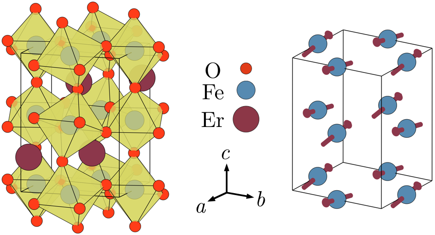
Figure 1: $Pnma$ lattice structure of $\text{ErFeO}_{3}$. The left unit cell shows the tilted octahedra of the distorted perovskite structure. The right unit cell shows the G-type antiferromagnetic ordering of the iron spins along the $a$ axis.

$\text{ErFeO}_{3}$ is a distorted perovskite with the orthorhombic $Pnma$ structure and the typical G-type antiferromagnetic ordering of the Fe³⁺ magnetic moments Treves (1965) (Fig. 1). The primitive magnetic unit cell contains 20 atoms, resulting in 60 phonon modes characterised by representations (within the orthorhombic point group $mmm$) $\text{A}_{\text{g}}$, $\text{B}_{(1,2,3)\text{g}}$, $\text{A}_{\text{u}}$ and $\text{B}_{(1,2,3)\text{u}}$. Of the polar “u” modes, only $\text{B}_{1\text{u}}$, $\text{B}_{2\text{u}}$ and $\text{B}_{3\text{u}}$ have dipole moments and are therefore excitable by mid-infrared light.

The totally symmetric representation in the $mmm$ point group is $\text{A}_{\text{g}}$, and so coupling is only symmetry allowed between combinations of phonon modes whose product contains the $\text{A}_{\text{g}}$ representation. To cubic order, and for excitation of the $\text{B}_{\text{u}}$ modes, this is the case for two types of mode combinations: quadratic-linear B${}_{i\text{u}}^{2}$A${}_{\text{g}}^{\phantom{i}}$ and trilinear $\text{B}_{i\text{u}}$$\text{B}_{j\text{u}}$$\text{B}_{k\text{g}}$, where $\{i,j,k\}=\{1,2,3\},i\neq{}j\neq{}k$. The quadratic-linear case describes the coupling of a single optically excited polar mode to a symmetric $\text{A}_{\text{g}}$ Raman mode, and is the nonlinear phononic scenario that has been studied previously Mankowsky et al. (2014); Först et al. (2013); Subedi et al. (2014); Mankowsky et al. (2015); Subedi (2015); Fechner and Spaldin (2016). In this work we focus instead on the trilinear case in which two IR modes with different symmetries are excited and combine with a $\text{B}_{k\text{g}}$ mode. We note also that in quartic order, any combination of infrared and Raman modes of the biquadratic form $Q_{\text{IR}}^{2}$$Q_{\text{R}}^{2}$ results in an $\text{A}_{\text{g}}$ representation, and so the potential energy up to fourth order can be written as:

$$V(\textbf{Q})= \frac{\omega_{1}^{2}}{2}Q_{\text{IR}_{1}}^{\phantom{2}}+\frac{\omega_{2}^{2}}{2}Q_{\text{IR}_{2}}^{\phantom{2}}+\frac{\omega_{\text{R}}^{2}}{2}Q_{\text{R}}^{\phantom{2}}+$$

$$c_{\text{R}}Q_{\text{R}}^{3}+c_{\text{1R}}Q_{\text{IR}_{1}}^{2}Q_{\text{R}}^{\phantom{2}}+c_{\text{2R}}Q_{\text{IR}_{2}}^{2}Q_{\text{R}}^{\phantom{2}}+$$

$$c_{\text{12R}}Q_{\text{IR}_{1}}^{\phantom{2}}Q_{\text{IR}_{2}}^{\phantom{2}}Q_{\text{R}}^{\phantom{2}}+$$ (1)

$$\frac{d_{\text{1}}}{4}Q_{\text{IR}_{1}}^{4}+\frac{d_{\text{2}}}{4}Q_{\text{IR}_{2}}^{4}+\frac{d_{\text{R}}}{4}Q_{\text{R}}^{4}+$$

$$d_{\text{12}}Q_{\text{IR}_{1}}^{2}Q_{\text{IR}_{2}}^{2}+d_{\text{1R}}Q_{\text{IR}_{1}}^{2}Q_{\text{R}}^{2}+d_{\text{2R}}Q_{\text{IR}_{2}}^{2}Q_{\text{R}}^{2},$$

where $Q_{\text{IR}_{1}}^{\phantom{2}}$ and $Q_{\text{IR}_{2}}^{\phantom{2}}$ denote the amplitudes of IR modes with different symmetries and eigenfrequencies $\omega_{1}$ and $\omega_{2}$ and $Q_{\text{R}}^{\phantom{2}}$ is the amplitude of a Raman mode with eigenfrequency $\omega_{\text{R}}$. The coefficients $\{c\}$ and $\{d\}$ define the strengths of the cubic and quartic anharmonicity and are material specific. As stated above, $c_{\text{R}}=c_{\text{1R}}=c_{\text{2R}}=0$ by symmetry if $Q_{\text{R}}^{\phantom{2}}$ corresponds to a $\text{B}_{i\text{g}}$ mode and $c_{\text{12R}}=0$ if $Q_{\text{R}}^{\phantom{2}}$ corresponds to an $\text{A}_{\text{g}}$ mode.

We will see that the quartic coefficients in ErFeO₃ are small, consistent with earlier work for related transition metal oxides Fechner and Spaldin (2016), and since we are interested in isolating the effects of the trilinear coupling, we analyze the reduced potential

$$V(\textbf{Q})= \frac{\omega_{1}^{2}}{2}Q_{\text{IR}_{1}}^{\phantom{2}}+\frac{\omega_{2}^{2}}{2}Q_{\text{IR}_{2}}^{\phantom{2}}+\frac{\omega_{\text{R}}^{2}}{2}Q_{\text{R}}^{\phantom{2}}+$$

$$c_{\text{12R}}Q_{\text{IR}_{1}}^{\phantom{2}}Q_{\text{IR}_{2}}^{\phantom{2}}Q_{\text{R}}^{\phantom{2}}$$ (2)

in the following. The value of $Q_{\text{R}}^{\phantom{2}}$ that minimizes $V(\textbf{Q})$, and which corresponds to the average structure induced by the trilinear coupling, is obtained trivially from this expression as

$$Q_{\text{R}_{\text{min}}}^{\phantom{2}}=\frac{c_{\text{12R}}Q_{\text{IR}_{1}}^{\phantom{2}}Q_{\text{IR}_{2}}^{\phantom{2}}}{\omega_{\text{R}}^{2}}.$$ (3)

We therefore expect that the induced structural distortions will be largest for low-frequency Raman modes with large $c_{\text{12R}}$ coupling coefficients.

We begin by calculating the structural properties of ErFeO₃ from first-principles within the density functional formalism as implemented in the Vienna ab-initio simulation package (VASP) Kresse and Furthmüller (1996a, b). We used the default VASP PAW pseudopotentials with valence electronic configurations Er (6$s^{2}$5$p^{6}$5$d^{1}$), Fe (3$d^{7}$4$s^{1}$) and O (2$s^{2}$2$p^{4}$), with the $4f$ electrons of erbium in the core. Treatment of the $4f$ electrons as core states has the desirable side effect of yielding the room-temperature magnetic structure, with the iron spins oriented along the $a$ axis and a weak ferromagnetic moment along $c$ Treves (1965) (Fig. 1), in our zero kelvin calculation, since the experimentally observed low-temperature spin-reorientation transitions to other easy axes White (1969), attributed to interaction with the Er $4f$ moments, are suppressed. Good convergence was obtained with a plane-wave energy cut-off of $850\,\text{eV}$ and a 6$\times$6$\times$4 $k$-point mesh to sample the Brillouin zone. We converged the Hellmann-Feynman forces to $10^{-5}\,\text{eV/$\text{\AA}${}}$ for the calculation of phonons with the frozen-phonon method as implemented in the phonopy package Togo and Tanaka (2015). For the exchange-correlation functional we chose the PBEsol Csonka et al. (2009) form of the generalized gradient approximation (GGA) with a Hubbard $U$ correction on the Fe $3d$ states. We found that an on-site Coulomb interaction of $U=3.7\,\text{eV}$ and a Hund’s exchange of $J=0.7\,\text{eV}$ optimally reproduce both the lattice dynamical properties Subba Rao et al. (1970); Koshizuka and Ushioda (1980); Nova et al. (2015) and the G-type antiferromagnetic ordering Treves (1965) as well as the photoemission spectrum of closely related LaFeO₃ Wadati et al. (2005). In particular we found that phonon eigenfrequencies are underestimated by other approaches, including the usual PBE functionals. Our fully relaxed structure with lattice constants $a=5.19\,\text{$\text{\AA}$}$, $b=5.56\,\text{$\text{\AA}$}$ and $c=7.52\,\text{$\text{\AA}$}$ fits reasonably well to the experimental values of Ref. Eibschütz (1965), as do our calculated phonon eigenfrequencies. Anharmonic coupling constants were computed by calculating the total energies as a function of ion displacements along the normal mode coordinates of every $Q_{\text{R}}^{\phantom{2}}$ mode and of every $Q_{\text{IR}_{1}}^{\phantom{2}}$ and $Q_{\text{IR}_{2}}^{\phantom{2}}$ modes that it couples to and then fitting the resulting three-dimensional energy landscape to the potential $V$ of Eqn. (Ultrafast Structure Switching through Nonlinear Phononics).

Table 1: Calculated and experimental phonon eigenfrequencies in THz. Infrared data were taken from Refs. Subba Rao et al. (1970); Nova et al. (2015), Raman data from Ref. Koshizuka and Ushioda (1980).

Sym.	DFT	Exp.	Sym.	DFT	Exp.
$\text{A}_{\text{g}}$	3.3	3.4	$\text{B}_{1\text{g}}$	3.2	3.4
	4.0	4.0		4.8	4.8
	8.1	8.1		9.6	9.7
	10.0	10.0		10.5	–
	12.5	12.4		14.6	15.1
	13.0	13.0		16.2	–
	14.9	14.9		18.3	–
$\text{B}_{2\text{u}}$	3.1	–	$\text{B}_{3\text{u}}$	3.5	–
	5.7	–		5.2	–
	7.2	–		7.5	–
	8.9	–		8.6	–
	9.7	–		9.9	–
	10.2	–		10.9	10.9
	13.2	13.3		12.4	–
	15.7	–		15.5	–
	16.0	16.2		16.5	17.0

In the experiment of Ref. Nova et al. (2015), the laser pulse was directed perpendicular to the short axes $a$ and $b$ of the orthorhombic $\text{ErFeO}_{3}$ crystal. The phonons that are excited by such a pulse have symmetries $\text{B}_{3\text{u}}$ (polarization along the $a$ axis) and $\text{B}_{2\text{u}}$ (polarization along the $b$ axis). The trilinear coupling term is therefore only nonzero for Raman modes of $\text{B}_{1\text{g}}$ symmetry; both IR modes couple quadratic-linearly to $\text{A}_{\text{g}}$ Raman modes. The experimental pulse frequency was $\omega_{0}=18.5\,\text{THz}$ with a pulse width of $\sigma_{\omega}=2.8\,\text{THz}$, so that IR modes between around 15 and 20 THz are significantly excited by the pulse. Our calculated values for the phonon eigenfrequencies with symmetries $\text{B}_{3\text{u}}$, $\text{B}_{2\text{u}}$, $\text{A}_{\text{g}}$ and $\text{B}_{1\text{g}}$ are listed in Tab. 1 (for the full list of calculated eigenfrequencies see the Appendix) along with available experimental values. In Fig. 2 a we show a model mid-infrared laser pulse with the properties of that used in Ref. Nova et al. (2015) and indicate our calculated $\text{B}_{3\text{u}}$ and $\text{B}_{2\text{u}}$ eigenfrequencies with vertical lines. We see that phonon modes with $\text{B}_{3\text{u}}$ and $\text{B}_{2\text{u}}$ symmetries occur in pairs of similar eigenfrequencies, consistent with the small orthorhombicity of $\text{ErFeO}_{3}$ (in a tetragonal structure they would form a pair of degenerate $\text{E}_{\text{u}}$ modes). It is also clear from Fig. 2 a that only the group of four IR modes with the highest eigenfrequencies $\text{B}_{3\text{u}}$(16.5), $\text{B}_{2\text{u}}$(16.0), $\text{B}_{2\text{u}}$(15.7) and $\text{B}_{3\text{u}}$(15.5) are significantly excited by the pulse of Ref. Nova et al. (2015). We show the displacements of the oxygen ions in the eigenvectors of these modes, and the direction of the corresponding polarization in Fig. 2 b–e. In the following analysis we focus on the two highest frequency modes, $\text{B}_{3\text{u}}$(16.5) and $\text{B}_{2\text{u}}$(16.0) and the lowest frequency Raman modes, $\text{B}_{1\text{g}}$(3.2) and $\text{A}_{\text{g}}$(3.3), for which we expect the biggest effect according to Eqn. (3).

Our calculated values for the anharmonic coefficients $\{c\}$ and $\{d\}$ for these modes are shown in Tab. 2 with the list of coefficients for the remaining combinations of the four highest frequency IR modes given in the Appendix. We see that the quartic order coupling coefficients between Raman and IR modes, $d_{\text{1R}}$ and $d_{\text{2R}}$ are all at least one order of magnitude smaller than the cubic coupling coefficients, $c_{\text{1R}}$, $c_{\text{2R}}$ and $c_{\text{12R}}$. (Note that the other anharmonic coefficents listed for completeness do not couple Raman and IR modes). This confirms our expectation that phonon-phonon coupling of the biquadratic kind is negligible for the dynamics of this system. We see also that the coefficient of trilinear coupling to the $\text{B}_{1\text{g}}$ mode is similar in magnitude (in fact slightly larger) to that of the quadratic-linear coupling to the $\text{A}_{\text{g}}$ mode.

Table 2: Anharmonic coefficients for the two Raman modes with lowest eigenfrequencies that couple to the $\text{B}_{3\text{u}}$(16.5) and $\text{B}_{2\text{u}}$(16.0) IR modes. Units are meV/$(\text{\AA}\sqrt{\mu})^{n}$, where $\mu$ is the atomic mass unit and $n$ the order of the phonon amplitude. The $\{c\}$ coefficients with 0 value vanish due to symmetry arguments, whereas $d_{\text{1R}}$ for the $\text{B}_{1\text{g}}$ mode is accidentally zero.

	$c_{\text{R}}$	$c_{\text{1R}}$	$c_{\text{2R}}$	$c_{\text{12R}}$	$d_{\text{1}}$	$d_{\text{2}}$	$d_{\text{R}}$	$d_{\text{12}}$	$d_{\text{1R}}$	$d_{\text{2R}}$
$\text{B}_{1\text{g}}$(3.2)	0	0	0	$-$10.2	17.6	8.2	1.1	12.0	0.0	$-$0.1
$\text{A}_{\text{g}}$ (3.3)	$-$0.5	7.8	3.7	0	17.6	8.2	1.1	12.0	$-$0.3	0.1

$-20$

$20$

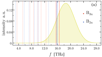
X

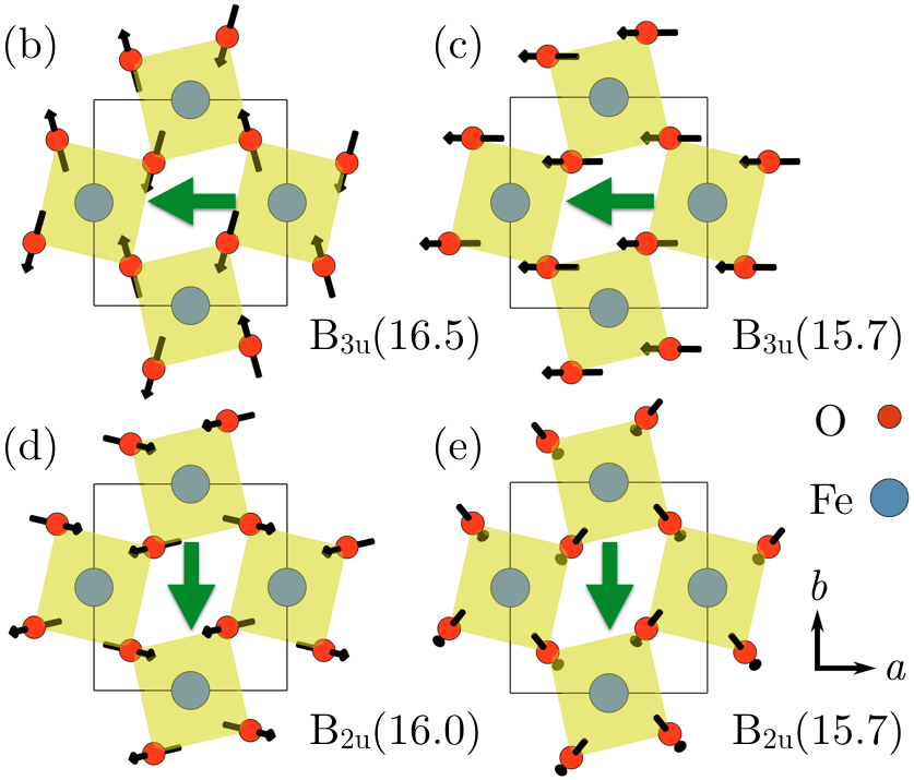
Figure 2: (a) Frequency spectrum of a model pump pulse with mean frequency $\omega_{0}=18.5\,\text{THz}$ and a full width at half maximum of $6.5\,\text{THz}$ as used in Ref. Nova et al. (2015). Our calculated phonon eigenfrequencies for $\text{ErFeO}_{3}$ are shown as vertical dashed lines, with the four highest frequency modes that we consider in this work marked as thicker dashed lines. The right panels show the displacements of the oxygen ions in modes (b) $\text{B}_{3\text{u}}$(16.5), (c) $\text{B}_{2\text{u}}$(16.0), (d) $\text{B}_{2\text{u}}$(15.7) and (e) $\text{B}_{3\text{u}}$(15.5) as thin black arrows and the resulting direction of polarization as thick green arrows.

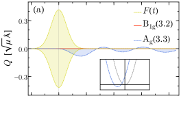
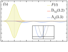
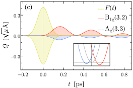
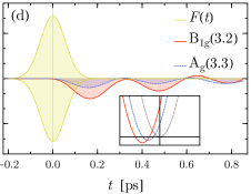
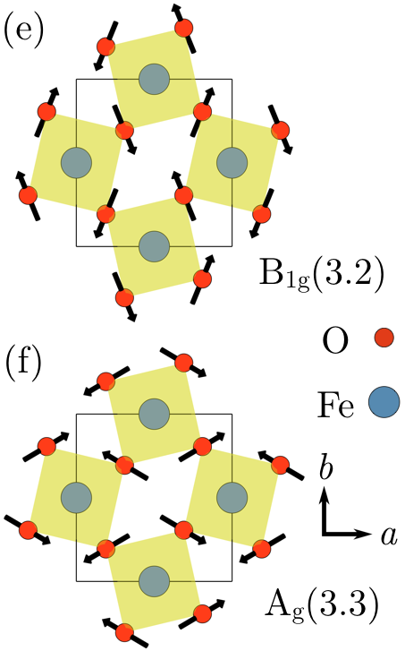
Figure 3: Evolution of the two Raman modes with lowest eigenfrequencies when pumped with linearly-polarized light at (a) $\theta=0^{\circ}$, (b) $\theta=90^{\circ}$, (c) $\theta=+45^{\circ}$ and (d) $\theta=-45^{\circ}$, with $\theta=0^{\circ}$ corresponding to a polarization along the $a$ axis of the crystal and $\theta=90^{\circ}$ to a polarization along the $b$ axis. We assumed a realistic linewidth of $\gamma\approx{}f/20$ Nova et al. (2015). The shifts in the minima of the Raman modes are shown schematically in the insets, with the gray curve indicating an unshifted potential, and blue and red the shifted $\text{A}_{\text{g}}$ and $\text{B}_{1\text{g}}$ potential respectively. The right panel shows the displacements of the oxygen ions corresponding to the modes (e) $\text{B}_{1\text{g}}$(3.2) and (f) $\text{A}_{\text{g}}$(3.3).

To investigate the evolution of the anharmonic system, we next solve numerically the dynamical equations of motion that form the system of coupled differential equations:

$$\ddot{\textbf{Q}}+\gamma\dot{\textbf{Q}}+\nabla_{\textbf{Q}}\left[V(\textbf{Q})-F(t,\theta)Q_{\text{IR}}^{\phantom{2}}{}\right]=0,$$ (4)

where $\textbf{Q}=(Q_{\text{IR}_{1}}^{\phantom{2}}{},Q_{\text{IR}_{2}}^{\phantom{2}}{},Q_{\text{R}}^{\phantom{2}}{})$ describes both the excited IR modes and one coupled Raman mode. $\gamma$ is the linewidth (inverse lifetime) of each mode and $F(t)$ the driving force on the IR modes that represents the laser pulse. We model the laser pulse with both time and frequency broadening as

$$F(t,\theta{})=F_{0}h(t,t_{0})\cos(\theta)\int\limits_{-\infty}^{\infty}\text{d}\omega\sin(\omega{}t)h(\omega{},\omega_{0}),$$ (5)

where $F_{0}$ is the maximum intensity and $h(x,x_{0})=\text{e}_{\text{\phantom{X}}}^{-(x-x_{0})^{2}/(2\sigma_{x}^{2})}/(\sqrt{2\pi}\sigma_{x})$ provides a gaussian spread both in time ($x=t$) and frequency ($x=\omega$). To conform to the experiment of Ref. Nova et al. (2015) we set the pulse duration to $\sigma_{t}=55\,\text{fs}$ and the frequency broadening to $\sigma_{\omega}=2.8\,\text{THz}$ at a mean frequency of $\omega_{0}=18.5\,\text{THz}$ with a peak amplitude of $F_{0}=10\,\text{MV/cm}$. $\theta$ is the polarization angle of the linearly-polarized light from the laser with respect to the symmetry of the IR modes with $\theta=0^{\circ}$ corresponding to a polarization along the $a$ axis of the crystal and $\theta=90^{\circ}$ to a polarization along the $b$ axis. The evolution of the system after an excitation with the laser pulse is shown in Fig. 3 a–d for a range of polarization angles. The displacements of the oxygen ions corresponding to the $\text{B}_{1\text{g}}$(3.2) and $\text{A}_{\text{g}}$(3.3) Raman modes are shown in Fig. 3 e, f.

In Fig. 3 a and b the polarization of the light pulse is along one of the lattice vectors so that in each case only IR modes of one symmetry type are excited, $\text{B}_{3\text{u}}$ in a, where the pulse is oriented along the $a$ axis ($\theta=0^{\circ}$) and $\text{B}_{2\text{u}}$ in b, for a pulse along the $b$ axis ($\theta=90^{\circ}$). As a result there is no trilinear coupling and no excitation of the $\text{B}_{1\text{g}}$(3.2) mode. In both cases, the $\text{A}_{\text{g}}$(3.3) mode is excited through its quadratic-linear coupling to the single IR mode. We see that its sinusoidal oscillation (blue line) is not centered around zero amplitude indicating the characteristic transient structural distortion caused by the quadratic-linear coupling $Q_{\text{IR}}^{2}$$Q_{\text{R}}^{\phantom{2}}$, as observed previously in Refs. Först et al. (2013); Mankowsky et al. (2015); Subedi et al. (2014); Subedi (2015); Fechner and Spaldin (2016) and described above. The induced shifts of the minimum in the potential for the Raman mode are shown in the insets. Since the potential depends quadratically on the IR mode, and the signs of the coupling coefficients $c_{\text{1R}}$ and $c_{\text{2R}}$ are the same, the direction of the structural distortion is independent of the angle of its polarization, with the same direction of shift for $\theta=0^{\circ}$ and $\theta=90^{\circ}$. Note, however, that the strength of the quadratic-linear coupling as different in the two cases, since the values of the coupling coefficients $c_{\text{1R}}$ and $c_{\text{2R}}$ differ.

In Fig. 3 c and d the polarization of the light pulse is midway between the lattice vectors, at $\theta=+45^{\circ}$ and $\theta=-45^{\circ}$ respectively so that both IR modes are excited simultaneously. In this case the response of the $\text{B}_{1\text{g}}$ mode is maximal. The behavior of the $\text{A}_{\text{g}}$ mode is the same as the previous cases, with the amplitude and direction of the shift in the average value independent of the polarization of the pulse. The trilinear coupling $Q_{\text{IR}_{1}}^{\phantom{2}}$$Q_{\text{IR}_{2}}^{\phantom{2}}$$Q_{\text{R}}^{\phantom{2}}$ of the $\text{B}_{1\text{g}}$(3.2) mode shows strikingly a different behaviour, however. We see that when the polarization angle is changed from $\theta=+45^{\circ}$ to $\theta=-45^{\circ}$, the trilinear coupling term changes sign and the transient deformation of the lattice is in the opposite direction along the the normal mode coordinates of the $\text{B}_{1\text{g}}$ mode.

The time for which the transient structural deformation of the $\text{B}_{1\text{g}}$ mode maintains its initial direction is determined by the inverse difference frequency $|\omega_{1}-\omega_{2}|^{-1}$, which determines the time-scale of the dephasing. The smaller the difference frequency the IR modes, the longer it takes them to dephase and thus the longer the directional selectivity of the trilinear coupling persists. For the realistic linewidth that we assumed, the structure relaxes back to the ground state before the IR modes dephase noticeably. In the case of a tetragonal structure in which the in-plane IR modes form a degenerate $\text{E}_{\text{u}}$ pair, $\omega_{1}=\omega_{2}$ and no dephasing occurs. In this limit both quadratic-linear and trilinear coupling to a fully symmetric $\text{A}_{\text{1g}}$ Raman mode should occur simultaneously, with their relative strengths determined by the angle of the excitation pulse to the crystallographic axes.

In summary, we have shown that excitation of two infrared-active (IR) phonon modes with different symmetries but similar eigenfrequencies in the orthorhombic perovskite ErFeO₃ causes a transient structural distortion along the eigenvectors of a coupled $\text{B}_{1\text{g}}$ Raman mode as a result of its trilinear coupling with the IR modes. In contrast to the quadratic-linear coupling of a symmetric $\text{A}_{\text{g}}$ Raman mode to a single IR mode that has been discussed previously Mankowsky et al. (2014); Först et al. (2013); Subedi et al. (2014); Mankowsky et al. (2015); Subedi (2015); Fechner and Spaldin (2016) and which we also observe here, the direction of the transient distortion is determined by the polarization of the excitation pulse relative to the crystallographic axes and can be reversed by reversing the polarization direction. While the analysis presented here was performed for ErFeO₃, it is directly applicable to all orthorhombic and tetragonal perovskites, with the strengths of the coupling constants and the values of the phonon frequencies of course being material dependent; extension to other crystal classes involves a further straightforward symmetry analysis. Our results suggest that nonlinear phononics can be used to control and switch the orientation of induced transient crystal structures.

We thank T. Nova and A. Cavalleri for fruitful discussions. This work was supported by the ETH Zürich and by the ERC Advanced Grant program, No. 291151. Calculations were performed at the Swiss National Supercomputing Centre (CSCS) supported by the project IDs s624 and p504.

*

Appendix

In Tab. 3 we show the full list of anharmonic coefficients used in this work. Note that the values may vary slightly for different mappings of the energy landscape due to the finite grid size. For example $d_{\text{1}}$ for the $\text{B}_{3\text{u}}$(16.5) mode is $17.6\,\text{meV/$(\text{\AA}\sqrt{\mu})^{n}$}$ when calculated together with $\text{B}_{2\text{u}}$(16.0) and $\text{B}_{1\text{g}}$(3.2), but $17.2\,\text{meV/$(\text{\AA}\sqrt{\mu})^{n}$}$ together with $\text{B}_{2\text{u}}$(16.0) and $\text{B}_{1\text{g}}$(3.2). For the dynamical equations of motion we used the average of these values. In Tab. 4 we show the full list of calculated eigenfrequencies in units of terahertz and inverse centimetres.

Table 3: Full list of anharmonic coefficients for the two Raman modes with lowest eigenfrequencies that couple to the four infrared modes with highest eigenfrequencies. Units are meV/$(\text{\AA}\sqrt{\mu})^{n}$, where $\mu$ is the atomic mass unit and $n$ the order of the phonon amplitude.

	$c_{\text{R}}$	$c_{\text{1R}}$	$c_{\text{2R}}$	$c_{\text{12R}}$	$d_{\text{1}}$	$d_{\text{2}}$	$d_{\text{R}}$	$d_{\text{12}}$	$d_{\text{1R}}$	$d_{\text{2R}}$
$Q_{\text{IR}_{1}}^{\phantom{2}}$=$\text{B}_{3\text{u}}$(16.5), $Q_{\text{IR}_{2}}^{\phantom{2}}$=$\text{B}_{2\text{u}}$(16.0)
$\text{B}_{1\text{g}}$(3.2)	0	0	0	$-$10.2	17.6	8.2	1.1	12.0	0.0	$-$0.1
$\text{A}_{\text{g}}$ (3.3)	$-$0.5	7.8	3.7	0	17.6	8.2	1.1	12.0	$-$0.3	0.1
$Q_{\text{IR}_{1}}^{\phantom{2}}$=$\text{B}_{3\text{u}}$(16.5), $Q_{\text{IR}_{2}}^{\phantom{2}}$=$\text{B}_{2\text{u}}$(15.7)
$\text{B}_{1\text{g}}$(3.2)	0	0	0	6.5	17.2	3.1	0.6	8.4	0.1	0.1
$\text{A}_{\text{g}}$ (3.3)	$-$0.4	7.6	5.9	0	17.3	3.1	0.6	8.3	$-$0.2	$-$0.1
$Q_{\text{IR}_{1}}^{\phantom{2}}$=$\text{B}_{3\text{u}}$(15.5), $Q_{\text{IR}_{2}}^{\phantom{2}}$=$\text{B}_{2\text{u}}$(16.0)
$\text{B}_{1\text{g}}$(3.2)	0	0	0	$-$18.0	22.9	6.8	0.2	8.5	0.8	0.1
$\text{A}_{\text{g}}$ (3.3)	$-$0.6	0.8	3.8	0	23.0	6.9	0.4	8.4	0.4	0.2
$Q_{\text{IR}_{1}}^{\phantom{2}}$=$\text{B}_{3\text{u}}$(15.5), $Q_{\text{IR}_{2}}^{\phantom{2}}$=$\text{B}_{2\text{u}}$(15.7)
$\text{B}_{1\text{g}}$(3.2)	0	0	0	$-$22.0	22.8	2.3	0.0	8.5	0.8	0.3
$\text{A}_{\text{g}}$ (3.3)	$-$0.3	0.3	5.6	0	22.8	2.3	0.1	8.5	0.4	0.0

$-25$

$25$

Table 4: Full list of calculated phonon frequencies.

#	THz	cm-1	Sym.	#	THz	cm-1	Sym.
1	0	0	acoust.	31	9.7	324	$\text{B}_{2\text{u}}$
2	0	0	acoust.	32	9.9	331	$\text{B}_{3\text{u}}$
3	0	0	acoust.	33	10.0	332	$\text{A}_{\text{g}}$
4	2.2	75	$\text{A}_{\text{u}}$	34	10.2	339	$\text{B}_{2\text{u}}$
5	3.1	103	$\text{B}_{2\text{u}}$	35	10.5	349	$\text{B}_{1\text{g}}$
6	3.2	107	$\text{B}_{1\text{g}}$	36	10.8	361	$\text{B}_{1\text{u}}$
7	3.3	111	$\text{A}_{\text{g}}$	37	10.9	364	$\text{B}_{3\text{u}}$
8	3.5	117	$\text{B}_{3\text{u}}$	38	10.9	365	$\text{B}_{3\text{g}}$
9	3.6	119	$\text{B}_{2\text{g}}$	39	11.1	370	$\text{A}_{\text{u}}$
10	3.9	129	$\text{B}_{3\text{g}}$	40	12.4	414	$\text{B}_{3\text{u}}$
11	4.0	134	$\text{A}_{\text{g}}$	41	12.5	416	$\text{A}_{\text{g}}$
12	4.7	155	$\text{B}_{1\text{u}}$	42	12.8	427	$\text{B}_{3\text{g}}$
13	4.7	158	$\text{A}_{\text{u}}$	43	12.9	432	$\text{B}_{2\text{g}}$
14	4.8	160	$\text{B}_{1\text{g}}$	44	13.0	432	$\text{A}_{\text{g}}$
15	4.8	161	$\text{B}_{1\text{u}}$	45	13.2	442	$\text{B}_{2\text{u}}$
16	5.2	175	$\text{B}_{3\text{u}}$	46	13.9	465	$\text{B}_{2\text{g}}$
17	5.7	191	$\text{B}_{2\text{u}}$	47	14.5	484	$\text{A}_{\text{u}}$
18	5.9	196	$\text{A}_{\text{u}}$	48	14.6	487	$\text{B}_{1\text{g}}$
19	7.0	232	$\text{A}_{\text{u}}$	49	14.8	494	$\text{B}_{1\text{u}}$
20	7.2	240	$\text{B}_{2\text{u}}$	50	14.9	496	$\text{A}_{\text{g}}$
21	7.5	250	$\text{B}_{3\text{u}}$	51	15.5	518	$\text{B}_{3\text{u}}$
22	7.7	257	$\text{B}_{1\text{u}}$	52	15.7	524	$\text{B}_{2\text{u}}$
23	7.7	257	$\text{B}_{3\text{g}}$	53	15.8	525	$\text{A}_{\text{u}}$
24	8.1	269	$\text{A}_{\text{g}}$	54	15.8	527	$\text{B}_{1\text{u}}$
25	8.6	288	$\text{B}_{3\text{u}}$	55	16.0	532	$\text{B}_{2\text{u}}$
26	8.9	296	$\text{B}_{2\text{u}}$	56	16.2	540	$\text{B}_{1\text{g}}$
27	9.2	306	$\text{A}_{\text{u}}$	57	16.5	551	$\text{B}_{3\text{u}}$
28	9.3	309	$\text{B}_{1\text{u}}$	58	18.3	612	$\text{B}_{1\text{g}}$
29	9.4	313	$\text{B}_{2\text{g}}$	59	18.4	614	$\text{B}_{3\text{g}}$
30	9.6	320	$\text{B}_{1\text{g}}$	60	19.3	645	$\text{B}_{2\text{g}}$

References

- Rini et al. (2007) M. Rini, R. Tobey, N. Dean, J. Itatani, Y. Tomioka, Y. Tokura, R. W. Schoenlein, and A. Cavalleri, Nature 449, 72 (2007).
- Tobey et al. (2008) R. I. Tobey, D. Prabhakaran, A. T. Boothroyd, and A. Cavalleri, Phys. Rev. Lett. 101, 197404 (2008).
- Beaud et al. (2009) P. Beaud, S. L. Johnson, E. Vorobeva, U. Staub, R. A. De Souza, C. J. Milne, Q. X. Jia, and G. Ingold, Phys. Rev. Lett. 103, 155702 (2009).
- Caviglia et al. (2012) A. D. Caviglia, R. Scherwitzl, P. Popovich, W. Hu, H. Bromberger, R. Singla, M. Mitrano, M. C. Hoffmann, S. Kaiser, P. Zubko, S. Gariglio, J. M. Triscone, M. Först, and A. Cavalleri, Phys. Rev. Lett. 108, 136801 (2012).
- Fausti et al. (2011) D. Fausti, R. I. Tobey, N. Dean, S. Kaiser, A. Dienst, M. C. Hoffmann, S. Pyon, T. Takayama, H. Takagi, and A. Cavalleri, Science 331, 189 (2011).
- Hu et al. (2014) W. Hu, S. Kaiser, D. Nicoletti, C. R. Hunt, I. Gierz, M. C. Hoffmann, M. Le Tacon, T. Loew, B. Keimer, and A. Cavalleri, Nat. Mater. 13, 705 (2014).
- Först et al. (2011) M. Först, C. Manzoni, S. Kaiser, Y. Tomioka, Y. Tokura, R. Merlin, and A. Cavalleri, Nat. Phys. 7, 854 (2011).
- Mankowsky et al. (2014) R. Mankowsky, A. Subedi, M. Först, S. O. Mariager, M. Chollet, H. T. Lemke, J. S. Robinson, J. M. Glownia, M. P. Minitti, A. Frano, M. Fechner, N. A. Spaldin, T. Loew, B. Keimer, A. Georges, and A. Cavalleri, Nature 516, 71 (2014).
- Först et al. (2013) M. Först, R. Mankowsky, H. Bromberger, D. M. Fritz, H. Lemke, D. Zhu, M. Chollet, Y. Tomioka, Y. Tokura, R. Merlin, J. P. Hill, S. L. Johnson, and A. Cavalleri, Solid State Commun. 169, 24 (2013).
- Mankowsky et al. (2015) R. Mankowsky, M. Först, T. Loew, J. Porras, B. Keimer, and A. Cavalleri, Phys. Rev. B 91, 094308 (2015).
- Fechner and Spaldin (2016) M. Fechner and N. A. Spaldin, arXiv:1607.01180 (2016).
- Nova et al. (2015) T. F. Nova, A. Cartella, A. Cantaluppi, M. Foerst, D. Bossini, R. V. Mikhaylovskiy, A. V. Kimel, R. Merlin, and A. Cavalleri, arXiv:1512.06351 (2015).
- Treves (1965) D. Treves, J. Appl. Phys. 36, 1033 (1965).
- Subedi et al. (2014) A. Subedi, A. Cavalleri, and A. Georges, Phys. Rev. B 89, 220301 (2014).
- Subedi (2015) A. Subedi, Phys. Rev. B 92, 214303 (2015).
- Kresse and Furthmüller (1996a) G. Kresse and J. Furthmüller, Comput. Mat. Sci. 6, 15 (1996a).
- Kresse and Furthmüller (1996b) G. Kresse and J. Furthmüller, Phys. Rev. B 54, 11169 (1996b).
- White (1969) R. L. White, J. Appl. Phys. 40, 1061 (1969).
- Togo and Tanaka (2015) A. Togo and I. Tanaka, Scr. Mater. 108, 1 (2015).
- Csonka et al. (2009) G. I. Csonka, J. P. Perdew, A. Ruzsinszky, P. H. T. Philipsen, S. Lebègue, J. Paier, O. A. Vydrov, and J. G. Ángyán, Phys. Rev. B 79, 155107 (2009).
- Subba Rao et al. (1970) G. V. Subba Rao, C. N. R. Rao, and J. R. Ferraro, Appl. Spectrosc. 24, 436 (1970).
- Koshizuka and Ushioda (1980) N. Koshizuka and S. Ushioda, Phys. Rev. B 22, 5394 (1980).
- Wadati et al. (2005) H. Wadati, D. Kobayashi, A. Chikamatsu, R. Hashimoto, M. Takizawa, K. Horiba, H. Kumigashira, T. Mizokawa, A. Fujimori, and M. Oshima, J. Electron. Spectrosc. Relat. Phenom. 147, 877 (2005).
- Eibschütz (1965) M. Eibschütz, Acta Cryst. 19, 337 (1965).
*