Lévy processes on a generalized fractal comb

Abstract

Comb geometry, constituted of a backbone and fingers, is one of the most simple paradigm of a two dimensional structure, where anomalous diffusion can be realized in the framework of Markov processes. However, the intrinsic properties of the structure can destroy this Markovian transport. These effects can be described by the memory and spatial kernels. In particular, the fractal structure of the fingers, which is controlled by the spatial kernel in both the real and the Fourier spaces, leads to the Lévy processes (Lévy flights) and superdiffusion. This generalization of the fractional diffusion is described by the Riesz space fractional derivative. In the framework of this generalized fractal comb model, Lévy processes are considered, and exact solutions for the probability distribution functions are obtained in terms of the Fox $H$-function for a variety of the memory kernels, and the rate of the superdiffusive spreading is studied by calculating the fractional moments. For a special form of the memory kernels, we also observed a competition between long rests and long jumps. Finally, we considered the fractional structure of the fingers controlled by a Weierstrass function, which leads to the power-law kernel in the Fourier space. It is a special case, when the second moment exists for superdiffusion in this competition between long rests and long jumps.

J. Phys. A: Math. Theor.

1 Introduction

A comb model is a particular example of a non-Markovian motion, which takes place due to its specific geometry realization inside a two dimensional structure. It consists of a backbone along the structure $x$ axis and fingers along the $y$ direction, continuously spaced along the $x$ coordinate, shown in Fig. 1. This special geometry has been introduced to investigate anomalous diffusion in low-dimensional percolation clusters [2, 29, 47, 49]. In the last decade the comb model has been extensively studied to understand different realizations of non-Markovian random walks, both continuous [1, 4, 13] and discrete [10]. In particular, comb-like models have been used to describe turbulent hyper-diffusion due subdiffusive traps [4, 21], anomalous diffusion in spiny dendrites [22, 32], subdiffusion on a fractal comb [19], and diffusion of light in Lévy glasses [3] as Lévy walks in quenched disordered media [8, 9], and to model anomalous transport in low-dimensional composites [43].

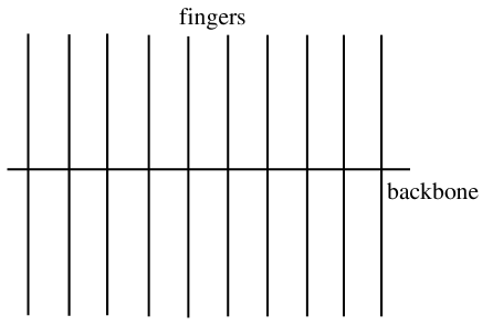
Figure 1: Comb-like structure.

The macroscopic model for the transport along a comb structure is presented by the following two-dimensional heterogeneous diffusion equation [2, 29, 47, 49]

$$\frac{\partial}{\partial t}P(x,y,t)=\mathcal{D}_{x}\delta(y)\frac{\partial^{2}}{\partial x^{2}}P(x,y,t)+\mathcal{D}_{y}\frac{\partial^{2}}{\partial y^{2}}P(x,y,t),$$ (1)

where $P(x,y,t)$ is the probability distribution function (PDF), $\mathcal{D}_{x}\delta(y)$ and $\mathcal{D}_{y}$ are diffusion coefficients in the $x$ and $y$ directions, respectively, with physical dimension $[\mathcal{D}_{x}]=\mathrm{m}^{3}/\mathrm{s}$, and $[\mathcal{D}_{y}]=\mathrm{m}^{2}/\mathrm{s}$. The $\delta(y)$ function (the Dirac $\delta(y)$ function) means that diffusion in the $x$ direction occurs only at $y=0$. This form of equations describes diffusion in the backbone (at $y=0$), while the fingers play the role of traps. Diffusion in a continuous comb can be described within the continuous time random walk (CTRW) theory [7]. For the continuous comb with infinite fingers, the returning probability scales like $t^{-1/2}$, and the waiting time PDF behaves as $t^{-3/2}$ [34], resulting in appearance of anomalous subdiffusion along the backbone with the transport exponent $1/2$. In another example of a fractal volume of an infinite number of backbones, it has been shown that the transport exponent depends on the fractal dimension of the backbone structure [40]. Natural phenomenological generalization of the comb model (1) is the generalization of both the time processes, by introducing memory kernels $\gamma(t)$ and $\eta(t)$, and introducing space inhomogeneous (fractal) geometry, i.e., a power-law density of fingers described by kernel $\rho(x)$ [19, 20, 22]. This modification of the comb model (1) can be expressed in the form of a so-called fractal comb model

$$\int_{0}^{t}dt^{\prime}\,\gamma(t-t^{\prime})\frac{\partial}{\partial t^{\prime}}P(x,y,t^{\prime}) =\mathcal{D}_{x}\delta(y)\int_{0}^{t}dt^{\prime}\,\eta(t-t^{\prime})\frac{\partial^{2}}{\partial x^{2}}P(x,y,t^{\prime})$$ (2)

$$+\mathcal{D}_{y}\frac{\partial^{2}}{\partial y^{2}}\int_{-\infty}^{\infty}dx^{\prime}\,\rho(x-x^{\prime})P(x^{\prime},y,t).$$

Here, the memory kernels $\gamma(t)$ and $\eta(t)$ are, in general case, decaying functions, approaching to zero in the long time limit (see [41] for details of the form of the memory kernels). The physical dimensions of the diffusion coefficients $\mathcal{D}_{x}\delta(y)$ and $\mathcal{D}_{y}$ depend now on the form of the memory kernels $\gamma(t)$ and $\eta(t)$. The memory kernels $\gamma(t)$ and $\eta(t)$, and the kernel $\rho(x)$ should be introduced in such a way that these functions do not change the physical meaning of the diffusion coefficients $\mathcal{D}_{x}\delta(y)$ and $\mathcal{D}_{y}$. Therefore, it is reasonable to introduce these functions in the dimensionless form, by introducing the time scale $\tau$ and the coordinate scale $l$. For example, it can be done in the following way [21]: $\tau=\mathcal{D}_{x}^{2}/\mathcal{D}_{y}^{3}$ and $l=\mathcal{D}_{x}/\mathcal{D}_{y}$, where we use that the dimension of $\mathcal{D}_{x}$ is $[\mathcal{D}_{x}]=l^{3}/\tau$, while the dimension of $\mathcal{D}_{y}$ is $[\mathcal{D}_{y}]=l^{2}/\tau$. This yields the corresponding change of the kernels $\gamma(t/\tau)$, $\eta(t/\tau)$, and $\rho(x/l)$, and this leads to the rescaling of Eq. (2). To avoid this procedure and keep the diffusion parameters $\mathcal{D}_{x}$ and $\mathcal{D}_{y}$ explicitly, we just state that the diffusion coefficients automatically absorb these scale parameters, and this rescaling depends on the functional form of $\gamma(t)$, $\eta(t)$ and $\rho(x)$. The function $\gamma(t)$ contributes to the memory effects in such a way that the particles moving along the $y$-direction, i.e., along the fingers, can be trapped. It means that diffusion along the $y$ direction can be anomalous as well [32, 39]. The function $\eta(t)$ is a so-called generalized compensation kernel [32]. The case $\gamma(t)=\eta(t)=\delta(t)$ yields the diffusion equation of the comb model (1). Corresponding CTRW models have been suggested, where the memory kernels appear in the waiting time [32, 41, 39]. A mesoscopic mechanism of this CTRW phenomenon has been suggested in [33], as well.

The spatial fractal geometry is taken into consideration by the fractal dimension of the finger volume (mass) $|x|^{\nu}$, where $0<\nu<1$ is the fractional dimension, and fingers are continuously distributed by the power-law. This can be presented as a convolution integral between the non-local density of fingers and the PDF $P(x,y,t)$ in the form [19] $\int_{-\infty}^{\infty}dx^{\prime}\,\rho(x-x^{\prime})P(x^{\prime},y,t)$, which also can be presented by the inverse Fourier transform $\mathcal{F}_{\kappa_{x}}^{-1}\left[|\kappa_{x}|^{1-\nu}\hat{P}(\kappa_{x},y,t)\right]$, where $\mathcal{F}_{x}\left[\rho(x)\right]=\tilde{\rho}\left(\kappa_{x}\right)=|\kappa_{x}|^{1-\nu}$. This integration also establishes a link between fractal geometry and fractional integro-differentiation [26, 36, 37] (see also the discussion in Summary).

As an illustration, a fractal comb is given in Fig. 2. The fractal comb in Fig. 2 is a random form of a middle third Cantor set construction, where a given segment with fingers is randomly divided in three parts and we delete the middle part. Therefore, we obtain the first generation which consists of two subsets of fingers. We repeat this middle third procedure for each subset to obtain the second generation with four random subsets of continuously distributed fingers. Then, one obtains the third generation, an so on. One should recognize that a random walk on this fractal comb (either random or regular) leads to correlations, related to quenched structures [7]. Therefore, the random structure of the comb induces correlation between successive trapping times in the fingers. In some cases of large scales, such random walks, can be renormalized to a CTRW model, and the quenched aspect can be neglected by using an effective trapping time PDF, as discussed in Ref. [7].

Figure 2: Fourth generation of a random one-third Cantor set. This fractal comb is a form of a middle third Cantor set construction [15], where each segment is randomly divided in three parts. The second slice is the first generation of the smallest part of the third generation of the Cantor set, shown in the upper slice.

Comb model (2) for $\nu=1$ reduces to a generalization of continuous comb model for anomalous and ultraslow diffusion. Furthermore, for $\gamma(t)=\eta(t)=\delta(t)$ the “classical” comb model (1) is recovered, as well. The anomalous diffusion processes are characterized by power-law dependence of the mean square displacement (MSD) on time $\left\langle x^{2}(t)\right\rangle\simeq t^{\alpha}$, where the anomalous diffusion exponent $\alpha$ is less than one for subdiffusive processes and greater than one for superdiffusive processes, see e.g. [35]. The comb model (2) for $\gamma(t)=\eta(t)=\frac{t^{-\mu}}{\Gamma(1-\mu)}$ ($0<\mu<1$) yields the fractional comb model considered in [22, 32], where the fractional derivatives appear in the form of the Caputo time fractional derivative

$${{}_{C}D_{t}^{q}}f(t)=\frac{1}{\Gamma(1-q)}\int_{0}^{t}dt^{\prime}\,(t-t^{\prime})^{-q}\frac{d}{dt^{\prime}}W(t^{\prime})$$ (3)

and the Riemman-Liouville fractional integral

$${{}_{RL}I_{t}^{q}}f(t)=\frac{1}{\Gamma(q)}\int_{0}^{t}dt^{\prime}\,(t-t^{\prime})^{q-1}f(t^{\prime}).$$ (4)

This paper is organized as follows. In Section 2 we give analytical results for generalized fractal comb model. Different memory kernels are used and anomalous superdiffusion is observed. The connection between fractal structure of fingers and the Riesz fractional derivative is presented in Section 3. Summary is given in Section 4. At the end of the paper an additional material necessary for understanding of the main text is presented in Appendices. These relate to definitions and properties of the Mittag-Leffler, Fox $H$ and Weierstrass functions. Calculations of the PDFs and fractional moments are also presented in A. Here we stress that we perform exact analytical analysis throughout the whole manuscript.

2 Model formulation and solution

At the first step of the present analysis let us understand the role of the $\delta(y)$ function in the highly inhomogeneous diffusion coefficients in Eqs. (1) and (2). One should recognize that the singularity of the $x$ component of the diffusion coefficient results from the Liouville equation; it is the intrinsic transport property of the comb models (1) and (2). Note that this singularity of the diffusion coefficient relates to a non-zero flux along the $x$ coordinates. Let us consider the Liouville equation

$$\frac{\partial}{\partial t}P+\mathrm{div}\,\mathbf{j}=0,$$ (5)

where the two dimensional current $\mathbf{j}=(j_{x},\,j_{y})=\left(-\delta(y)\frac{\partial}{\partial x}P,\,-\frac{\partial}{\partial y}P\right)$ describes Markov processes in Eq. (1). However, diffusion in both the backbone and fingers can be in general non-Markovian processes, which is reflected in Eq. (2). Moreover the fingers can be inhomogeneously distributed as occurs in dendritic spines, where the spines are randomly (rather than uniformly) distributed [16]. In this case the two-dimensional current reads

$$j_{x}=-\mathcal{D}_{x}\delta(y)\int dt^{\prime}\eta^{\prime}(t-t^{\prime})\frac{\partial}{\partial x}P(x,y,t^{\prime}),$$ (6)

$$j_{y}=-\mathcal{D}_{y}\int dx^{\prime}dt^{\prime}\gamma^{\prime}(t-t^{\prime})\rho(x-x^{\prime})\frac{\partial}{\partial y}P(x^{\prime},y,t^{\prime}).$$ (7)

Eq. (5) together with Eqs. (6) and (7), can be regarded as the two-dimensional non-Markovian master equation. Integrating Eq. (5) over $y$ from $-\epsilon/2$ to $\epsilon/2$: $\int_{-\epsilon/2}^{\epsilon/2}dy\dots$, one obtains for the l.h.s. of the equation, after application of the middle point theorem, $\epsilon\frac{\partial}{\partial t}P(x,y=0,t)$, which is exact in the limit $\epsilon\rightarrow 0$. This term can be neglected in the limit $\epsilon\rightarrow 0$. Considering integration of the r.h.s. of the equation, we obtain that the term responsible for the transport in the $y$ direction reads from Eq. (7)

$$\int dt^{\prime}dx^{\prime}\gamma^{\prime}(t-t^{\prime})\rho(x-x^{\prime})\frac{\partial}{\partial y}\Big{[}P(x^{\prime},y,t^{\prime})\big{|}_{y=\epsilon/2}-P(x,y,t^{\prime})\big{|}_{y=-\epsilon/2}\Big{]}\,.$$

This corresponds to the two outgoing fluxes from the backbone in the $\pm y$ directions: $F_{y}(y=+0)+F_{y}(y=-0)$. The transport along the $x$ direction, after integration of Eq. (6), is

$$\epsilon\mathcal{D}(y\rightarrow 0)\frac{\partial^{2}}{\partial x^{2}}\int dt^{\prime}\eta^{\prime}(t-t^{\prime})P(x,y=0,t^{\prime})=F_{x}(x+\epsilon)+F_{x}(x-\epsilon)\,.$$

Here, we take a general diffusivity function in the $x$ direction $\mathcal{D}(y)$ (instead of $\mathcal{D}_{x}\delta(y)$ in Eq. (5) and (6)). It should be stressed that the second derivative over $x$, presented in the form $\epsilon\frac{\partial^{2}}{\partial x^{2}}P=\left[\frac{\partial}{\partial x}P(x+\epsilon/2)-\frac{\partial}{\partial x}P(x-\epsilon/2)\right]$ as $\epsilon\rightarrow 0$, ensures both incoming and outgoing fluxes for $F_{x}$ along the $x$ direction at a point $x$. After integration over $y\in[-\epsilon,+\epsilon]$, the Liouville equation is a kind of the Kirchhoff’s law: $F_{x}(+)+F_{x}(-)+F_{y}(+)+F_{y}(-)=0$ for each point $x$ and at $y=0$. Since $j_{x}\neq 0$, outgoing fluxes are not zero, the flux $F_{x}\equiv F_{x}(+)+F_{x}(-)$ has to be nonzero as well: $F_{x}(\pm)\neq 0$. Therefore, $\epsilon D(y\rightarrow 0)\neq 0$. Taking the diffusion coefficient in the form $\mathcal{D}(y)=\frac{1}{\pi}\frac{\epsilon\mathcal{D}_{x}}{y^{2}+\epsilon^{2}}$, one obtains in the limit $\epsilon\rightarrow 0$ a nonzero flux $F_{x}$ with $\mathcal{D}(y)=\mathcal{D}_{x}\delta(y)$, which is the diffusion coefficient in the $x$ direction in Eqs. (2), (5) and (6). The relations between kernels $\gamma(t)$, $\eta(t)$ and $\gamma^{\prime}(t)$, and $\eta^{\prime}(t)$ in Eqs. (2) and (5), (6) and (7) can be established in the Laplace space. Namely, performing the variable change in the Laplace space $\mathcal{L}[\gamma(t)]=\mathcal{L}[\gamma^{\prime}(t)]$ and $\mathcal{L}[\eta(t)]=\mathcal{L}[\eta^{\prime}(t)]/\mathcal{L}[\gamma^{\prime}(t)]$ one arrives at Eq. (2).

Presenting the last term in Eq. (2) in the Fourier inversion form, Eq. (2) reads

$$\int_{0}^{t}dt^{\prime}\,\gamma(t-t^{\prime})\frac{\partial}{\partial t^{\prime}}P(x,y,t^{\prime}) =\mathcal{D}_{x}\delta(y)\int_{0}^{t}dt^{\prime}\,\eta(t-t^{\prime})\frac{\partial^{2}}{\partial x^{2}}P(x,y,t^{\prime})$$ (8)

$$+\mathcal{D}_{y}\mathcal{F}_{\kappa_{x}}^{-1}\left[|\kappa_{x}|^{1-\nu}\frac{\partial^{2}}{\partial y^{2}}\tilde{P}(\kappa_{x},y,t)\right],$$

where $\rho(x)\sim|x|^{\nu-2}$ is used. Therefore, Eq. (8) can be presented by means of the Riesz space fractional derivative $\frac{\partial^{1-\nu}}{\partial|x|^{1-\nu}}$ of order $0<1-\nu<1$ [38]. This fractional derivative appears as a result of presenting the fingers density $|x|^{\nu-1}$ in the form of the Fourier transform. This natural generalization of Eq. (8) establishes a relation between the fractal geometry of the medium and fractional integro-differentiation, where the reciprocal fractional density $|\kappa_{x}|^{1-\nu}$ leads to the fractional Riesz derivative of the order $0<1-\nu<1$. We also admit here that for $\nu=1$ ($\rho(x)=\delta(x)$) we call Eq. (2) and Eq. (8) “continuous” comb, while for $\nu<1$ it is “fractal” comb model.

2.1 PDF and $q$-th moment along the backbone

To understand the properties of anomalous diffusion, one calculates the MSD. However, the MSD can diverge for Lévy processes. In this case one calculates a fractional $q$-th moment, which is obtained here.

The Fourier-Laplace transforms of Eq. (8) yield

$$\hat{\gamma}(s)\left[s\tilde{\hat{P}}(\kappa_{x},\kappa_{y},s)-\tilde{P}(\kappa_{x},\kappa_{y},t=0)\right] =-\mathcal{D}_{x}\kappa_{x}^{2}\hat{\eta}(s)\tilde{\hat{P}}(\kappa_{x},y=0,s)$$ (9)

$$-\mathcal{D}_{y}|\kappa_{x}|^{1-\nu}\kappa_{y}^{2}\tilde{\hat{P}}(\kappa_{x},\kappa_{y},s),$$

where $\tilde{\hat{P}}(\kappa_{x},y,s)=\mathcal{F}_{x}\left[\mathcal{L}\left[P(x,y,t)\right]\right]$ and $\tilde{\hat{P}}(\kappa_{x},\kappa_{y},s)=\mathcal{F}_{y}\left[\tilde{\hat{P}}(\kappa_{x},y,s)\right]$. Performing the inverse Fourier transform of $\tilde{\hat{P}}(\kappa_{x},\kappa_{y},s)$ with respect to $\kappa_{y}$, one finds $\tilde{\hat{P}}(\kappa_{x},y,s)$, from where $\tilde{\hat{P}}(\kappa_{x},y=0,s)$ reads

$$\tilde{\hat{P}}(\kappa_{x},y=0,s)=\left.\frac{1}{s}\sqrt{\frac{s\hat{\gamma}(s)}{4\mathcal{D}_{y}}}|\kappa_{x}|^{\frac{\nu-1}{2}}\right/\left[1+\frac{1}{s}\sqrt{\frac{s\hat{\gamma}(s)}{4\mathcal{D}_{y}}}\frac{\mathcal{D}_{x}\hat{\eta}(s)}{\hat{\gamma}(s)}|\kappa_{x}|^{\frac{3+\nu}{2}}\right].$$ (10)

Here we use the initial condition $\tilde{P}(\kappa_{x},\kappa_{y},t=0)=1$. Substituting Eq. (10) in Eq. (9), one obtains

$$\tilde{\hat{P}}(\kappa_{x},\kappa_{y},s)=\frac{s\hat{\gamma}(s)\hat{\xi}(s)}{\left(s\hat{\gamma}(s)+\mathcal{D}_{y}|\kappa_{x}|^{1-\nu}\kappa_{y}^{2}\right)\left(s\hat{\xi}(s)+\frac{\mathcal{D}_{x}}{2\sqrt{\mathcal{D}_{y}}}|\kappa_{x}|^{\frac{3+\nu}{2}}\right)}.$$ (11)

Taking $\kappa_{y}=0$ in Eq. (11), which eventually leads to the reduced PDF $p_{1}(x,t)=\int_{-\infty}^{\infty}dy\,P(x,y,t)$, one obtains the latter in the form

$$\tilde{\hat{p}}_{1}(\kappa_{x},s)=\frac{\hat{\xi}(s)}{s\hat{\xi}(s)+\frac{\mathcal{D}_{x}}{2\sqrt{\mathcal{D}_{y}}}|\kappa_{x}|^{\frac{3+\nu}{2}}},$$ (12)

where $\tilde{\hat{p}}_{1}(\kappa_{x},s)=\mathcal{F}_{x}\left[\mathcal{L}\left[p_{1}(x,t)\right]\right]$, and

$$\hat{\xi}(s)=\frac{1}{\hat{\eta}(s)}\sqrt{\frac{\hat{\gamma}(s)}{s}}.$$ (13)

Equation (12) corresponds to the fractional diffusion equation for the reduced distribution $p_{1}(x,t)$, which describes both Lévy flights with traps and subdiffusion,

$$\int_{0}^{t}dt^{\prime}\,\xi(t-t^{\prime})\frac{\partial}{\partial t^{\prime}}p_{1}(x,t^{\prime})=\frac{\mathcal{D}_{x}}{2\sqrt{\mathcal{D}_{y}}}\frac{\partial^{\alpha}}{\partial|x|^{\alpha}}p_{1}(x,t).$$ (14)

Here the Riesz space fractional derivative is of order $\alpha=\frac{3+\nu}{2}\leq 2$, while integro-differentiation with respect to time is presented in the Caputo form.

Introducing a waiting times PDF $\psi(t)$, which in the Laplace space is given by $\hat{\psi}(s)=\left(1+s\hat{\xi}(s)\right)^{-1}$ [39], one obtains the relation $\hat{\xi}(s)=\frac{1-\hat{\psi}(s)}{s\hat{\psi}(s)}$. For example, in the Markov case, when $\psi(t)=\frac{1}{\tau}e^{-t/\tau}$, the trap kernel is a $\delta$ function and the l.h.s. of Eq. (14) reduces to the standard time derivative $\frac{\partial}{\partial t}p_{1}(x,t)$. A subdiffusive case, when $\psi(t)=\frac{1}{1+(t/\tau)^{\beta}}$, yields [23] $\hat{\xi}^{-1}(s)=s^{1-\beta}$. Then the l.h.s. of Eq. (14) corresponds to the Caputo fractional derivative of the order of $\beta$, defined in Eq. (3). Therefore, the power-law tail of the kernel $\xi(t)$ determines the Caputo fractional derivative (3).

It is worth mentioning that the solution of Eq. (8) in the Fourier-Laplace space $(\kappa_{x},s)$ can be written as

$$\tilde{\hat{P}}(\kappa_{x},y,s)=\exp\left(-\sqrt{\frac{s\tilde{\hat{g}}(\kappa_{x},s)}{\mathcal{D}_{y}}}|y|\right)\tilde{\hat{f}}(\kappa_{x},s),$$ (15)

where $f(x,t)$ and $g(x,t)$ are functions standing for the derivation. We find that $\tilde{\hat{g}}(\kappa_{x},s)=\hat{\gamma}(s)|\kappa_{x}|^{\nu-1}$ and $\tilde{\hat{f}}(\kappa_{x},s)$ is given by Eq. (10), from where the Fourier transform in respect to $y$, gives the same expression for $\tilde{\hat{P}}(\kappa_{x},\kappa_{y},s)$ as in Eq. (11).

The $q$-th fractional moments can be analyzed for various forms of the kernels $\gamma(t)$ and $\eta(t)$

$$\left\langle|x(t)|^{q}\right\rangle=2\int_{0}^{\infty}dx\,x^{q}p_{1}(x,t),$$ (16)

where $0<q<\alpha<2$. One considers the $q$-th fractional moments with $q<\alpha$, since the MSD for Lévy processes governed by equation (14) does not exist. Therefore, instead of the MSD one can analyze its analogue related to the $q$-th moment, $\left\langle|x(t)|^{q}\right\rangle^{2/q}$ [35]. From relation (12) one obtains

$$\left\langle|x(t)|^{q}\right\rangle=C_{\alpha}(q)\mathcal{L}^{-1}\left[\frac{1}{s\left(s\hat{\xi}(s)\right)^{q/\alpha}}\right],$$ (17)

where

$$C_{\alpha}(q)=\frac{4}{\alpha}\left(\frac{\mathcal{D}_{x}}{2\sqrt{\mathcal{D}_{y}}}\right)^{q/\alpha}\frac{\Gamma(q)\Gamma\left(1+q/\alpha\right)\Gamma\left(-q/\alpha\right)}{\Gamma(q/2)\Gamma(-q/2)}.$$ (18)

The case with $\nu=1$, i.e., $\alpha=2$ (continuous comb), yields

$$\left\langle|x(t)|^{q}\right\rangle=\Gamma(q+1)\left(\frac{\mathcal{D}_{x}}{2\sqrt{\mathcal{D}_{y}}}\right)^{q/2}\mathcal{L}^{-1}\left[\frac{1}{s\left(s\hat{\xi}(s)\right)^{q/2}}\right],$$ (19)

from where for $q=2$ we recover the result for the MSD [41]

$$\left\langle x^{2}(t)\right\rangle=\frac{\mathcal{D}_{x}}{\sqrt{\mathcal{D}_{y}}}\mathcal{L}^{-1}\left[\frac{1}{s^{2}\hat{\xi}(s)}\right].$$ (20)

Now setting different functional behaviors of the kernels $\gamma(t)$ and $\eta(t)$, one can observe various diffusion regimes, along both the $x$ and $y$ directions.

2.2 Special case I: Lévy distribution

When $\gamma(t)=\delta(t)$, i.e., $\hat{\gamma}(s)=1$, and $\eta(t)=\frac{t^{-1/2}}{\Gamma(1/2)}$, i.e., $\hat{\eta}(s)=s^{-1/2}$, which means $\hat{\xi}(s)=1$, we obtain the Markovian transport equation for superdiffusion along the backbone

$$\frac{\partial}{\partial t}p_{1}(x,t)=\frac{\mathcal{D}_{x}}{2\sqrt{\mathcal{D}_{y}}}\frac{\partial^{\alpha}}{\partial|x|^{\alpha}}p_{1}(x,t).$$ (21)

Taking the initial condition $p_{1}(x,0+)=\delta(x)$ and the boundary conditions $p_{1}(\pm\infty,t)=\frac{\partial}{\partial x}p_{1}(\pm\infty,t)=0$ (see A), one obtains the solution of Eq. (21)

$$p_{1}(x,t)=\frac{1}{\alpha|x|}H_{3,3}^{2,1}\left[\left.\frac{|x|}{\left(\frac{\mathcal{D}_{x}}{2\sqrt{\mathcal{D}_{y}}}t\right)^{1/\alpha}}\right|\left.\begin{array}[]{l}(1,\frac{1}{\alpha}),(1,\frac{1}{\alpha}),(1,\frac{1}{2})\\ (1,1),(1,\frac{1}{\alpha}),(1,\frac{1}{2})\end{array}\right.\right],$$ (24)

where $H_{p,q}^{m,n}\left[z\left|\begin{array}[]{l}(a_{p},A_{p})\\ (b_{q},B_{q})\end{array}\right.\right]$ is the Fox $H$-function [31] (see also a brief introduction in C).

Therefore, the $q$-th moment reads (see calculations in A)

$$\left\langle|x(t)|^{q}\right\rangle=C_{\alpha}(q)\frac{t^{q/\alpha}}{\Gamma\left(1+q/\alpha\right)},$$ (25)

where $C_{\alpha}(q)$ is defined in Eq. (18). From Eq. (25) one obtains $\left\langle|x(t)|^{q}\right\rangle^{2/q}\simeq t^{4/(3+\nu)}$ that corresponds to superdiffusion (Lévy flights [48]) since $0<\nu<1$. The same superdiffusive behavior is observed when $s^{-1/2}\sqrt{\hat{\gamma}(s)}=\hat{\eta}(s)$, which means $\hat{\xi}(s)=1$. Note that Eq. (9) describes a typical competition between long rests and long jumps [35]. Contrary to the case described in Refs. [19, 32], in the present analysis, superdiffusion can be dominant not only due to the fractional (power-law) distribution of the fingers with $0<\nu<1$, but also due to the specific choice of the time kernels $\eta(t)$ and $\gamma(t)$.

2.3 Special case II: Competition between long rests and Lévy flights

Now we consider the power-law memory kernels in the form $\gamma(t)=\eta(t)=\frac{t^{-\mu}}{\Gamma(1-\mu)}$, $0<\mu<1$. From Eq. (13) we find $\hat{\xi}(s)=s^{-\mu/2}$, which yields in the time domain that $\xi(t)=\frac{t^{-(1-\mu/2)}}{\Gamma(\mu/2)}$. Therefore, the space-time fractional diffusion equation for the reduced PDF $p_{1}(x,t)$ is a non-Markovian trasport equation for superdiffusion along the backbone

$${{}_{C}}D_{t}^{1-\mu/2}p_{1}(x,t)=\frac{\mathcal{D}_{x}}{2\sqrt{\mathcal{D}_{y}}}\frac{\partial^{\alpha}}{\partial|x|^{\alpha}}p_{1}(x,t),$$ (26)

where ${{}_{C}}D_{t}^{1-\mu/2}$ is the Caputo time fractional derivative (3) of order $1/2<1-\mu/2<1$, and $\frac{\partial^{\alpha}}{\partial|x|^{\alpha}}$ is the Riesz space fractional derivative of order $\alpha=\frac{3+\nu}{2}$. The initial condition is $p_{1}(x,0+)=\delta(x)$, and the boundary conditions are defined at infinities $p_{1}(\pm\infty,t)=\frac{\partial}{\partial x}p_{1}(\pm\infty,t)=0$. Taking into account the initial and the boundary conditions, one obtains the solution of Eq. (26) in terms of the Fox $H$-function (see A, Eq. (82))

$$p_{1}(x,t)=\frac{1}{\alpha|x|}H_{3,3}^{2,1}\left[\left.\frac{|x|}{\left(\frac{\mathcal{D}_{x}}{2\sqrt{\mathcal{D}_{y}}}t^{1-\mu/2}\right)^{1/\alpha}}\right|\left.\begin{array}[]{l}(1,\frac{1}{\alpha}),(1,\frac{1-\mu/2}{\alpha}),(1,\frac{1}{2})\\ (1,1),(1,\frac{1}{\alpha}),(1,\frac{1}{2})\end{array}\right.\right].$$ (29)

Repeating the calculation of the fractional $q$-th moment in Eq. (91), one obtains

$$\left\langle|x(t)|^{q}\right\rangle=C_{\alpha}(q)\frac{t^{\frac{2-\mu}{2\alpha}q}}{\Gamma\left(1+\frac{2-\mu}{2\alpha}q\right)},$$ (30)

which also yields $\left\langle|x(t)|^{q}\right\rangle^{2/q}\simeq t^{(2-\mu)/\alpha}$. One concludes here that superdiffusion appears for $2\mu+\nu<1$, and subdiffusion takes place for $2\mu+\nu>1$. These effects result from the combination of the memory kernels that eventually leads to the competition between long rests and long jumps. Note that in the limit case of $\nu=1$, there is subdiffusion with the correct MSD $\left\langle x^{2}(t)\right\rangle\simeq t^{1-\mu/2}$ [35, 42].

2.4 Special case III: Distributed order memory kernels

Note that there are many choices of the memory kernels that can lead to more specific situations. For example, as it is shown in Refs. [11, 27, 39], distributed order memory kernels can lead to a strong anomaly in fractional kinetics like ultra-slow diffusion, where for example the Sinai diffusion [45] is one of the best-known realizations of anomalous kinetics.

Let us consider the distributed order memory kernel of the form [11, 12, 24, 27]

$$\gamma(t)=\int_{0}^{1}d\mu\,\frac{t^{-\mu}}{\Gamma(1-\mu)},$$ (31)

which yields $\gamma(s)=\frac{s-1}{s\log(s)}$ [11, 27], and for $\eta(t)=\delta(t)$ one obtains $\xi(s)=\frac{1}{s}\sqrt{\frac{s-1}{\log{s}}}$. For the calculation of the $q$-th moment, it is convenient to use here the Tauberian theorem [17], which states that for a slowly varying function $L(t)$ at infinity, i.e., $\lim_{t\rightarrow\infty}\frac{L(at)}{L(t)}=1$, $a>0$, if $\hat{R}(s)\simeq s^{-\rho}L\left(\frac{1}{s}\right)$, $s\rightarrow 0$, $\rho\geq 0,$ then $r(t)=\mathcal{L}^{-1}\left[\hat{R}(s)\right]\simeq\frac{1}{\Gamma(\rho)}t^{\rho-1}L(t)$, $t\rightarrow\infty$. Therefore, applying the Tauberian theorem, one obtains the behavior of the fractional $q$-th moments in the long time limit

$$\left\langle|x(t)|^{q}\right\rangle=C_{\alpha}(q)\mathcal{L}^{-1}\left[\frac{1}{s}\left(\frac{\log{s}}{s-1}\right)^{\frac{q}{2\alpha}}\right]\simeq C_{\alpha}(q)\mathcal{L}^{-1}\left[\frac{1}{s}\left(\log{\frac{1}{s}}\right)^{\frac{2q}{\alpha}}\right]\simeq C_{\alpha}(q)\log^{\frac{q}{2\alpha}}t,$$ (32)

which yields $\left\langle|x(t)|^{q}\right\rangle^{2/q}\simeq\log^{\frac{1}{\alpha}}t$. This result also contains the correct limit of the continuous comb with $\nu=1$ ($\alpha=2$), when the MSD reads $\left\langle x^{2}(t)\right\rangle\simeq\frac{\mathcal{D}_{x}}{\sqrt{\mathcal{D}_{y}}}\log^{1/2}t$ [41]. It should be stressed that ultra-slow diffusion takes place here even in the presence of the Lévy flights. However the latter affects only the power of the logarithm, since ultra-slow diffusion is the robust process with respect to the inhomogeneous distribution of the fingers.

For a more general distributed order memory kernel of the form [12]

$$\gamma(t)=\int_{0}^{1}d\mu\,\lambda\mu^{\lambda-1}\frac{t^{-\mu}}{\Gamma(1-\mu)},$$ (33)

where $\lambda>0$, one obtains for the long time limit $\gamma(s)\simeq\frac{\Gamma(1+\lambda)}{s\log^{\lambda}\frac{1}{s}}$, and for $\eta(t)=\delta(t)$ the $q$-th moment reads

$$\left\langle|x(t)|^{q}\right\rangle\simeq C_{\alpha}(q)\mathcal{L}^{-1}\left[\frac{1}{s}\left(\frac{\log^{\lambda}{\frac{1}{s}}}{\Gamma(1+\lambda)}\right)^{\frac{q}{2\alpha}}\right]\simeq C_{\alpha}(q)\left(\frac{\log^{\lambda}t}{\Gamma(1+\nu)}\right)^{\frac{q}{2\alpha}}.$$ (34)

This $q$-th moment behavior eventually yields $\left\langle|x(t)|^{q}\right\rangle^{2/q}\simeq\left(\frac{\log^{\lambda}t}{\Gamma(1+\nu)}\right)^{1/\alpha}$, which also contains the limiting case of the continuous comb with the MSD $\left\langle x^{2}(t)\right\rangle\simeq\frac{\mathcal{D}_{x}}{\sqrt{\mathcal{D}_{y}}}\frac{\log^{\lambda/2}t}{\sqrt{\Gamma(1+\lambda)}}$ [41].

2.5 Diffusion along fingers

One easily finds that the solution (11) does not describe diffusion in the $y$ direction. Indeed, it follows from Eq. (11) that

$$\tilde{\hat{p}}_{2}(\kappa_{y},s)=\frac{1}{s},$$ (35)

where $p_{2}(y,t)=\int_{-\infty}^{\infty}dx\,P(x,y,t)$, which means that $p_{2}(y,t)=\delta(y)$, from where one obtains that the MSD along the $y$-direction is equal to zero. However diffusion in the $y$ direction does take place with the diffusivity $\mathcal{D}_{y}$. To resolve this paradox, one should understand that the MSD is obtained by averaging over the total volume, which yields zero power of the set: $\lim_{L\to\infty}\frac{1}{L}\int_{0}^{L}dx\,x^{\nu-1}\sim\lim_{L\to\infty}L^{\nu-1}=0$. To obtain a finite result, one has to average over the fractal volume $L^{\nu}$. Therefore, the Fourier inversion over the fractal measure $|\kappa_{x}|^{\nu-1}d\kappa_{x}$ yields for the MSD

$$\left\langle y^{2}(t)\right\rangle=\mathcal{L}^{-1}\left.\left[-\frac{\partial^{2}}{\partial\kappa_{y}^{2}}\tilde{\hat{P}}(\kappa_{x},\kappa_{y},s)|\kappa_{x}|^{\nu-1}\right]\right|_{\kappa_{x}=0,\kappa_{y}=0}$$

$$=\mathcal{L}^{-1}\left.\left[\frac{2\mathcal{D}_{y}s\hat{\gamma}(s)-6\mathcal{D}_{y}^{2}|\kappa_{x}|^{1-\nu}\kappa_{y}^{2}}{\left(s\hat{\gamma}(s)+\mathcal{D}_{y}|\kappa_{x}|^{1-\nu}\kappa_{y}^{2}\right)^{3}}\cdot\frac{s\hat{\gamma}(s)\hat{\xi}(s)}{s\hat{\xi}(s)+\frac{\mathcal{D}_{x}}{2\sqrt{\mathcal{D}_{y}}}|\kappa_{x}|^{\frac{3+\nu}{2}}}\right]\right|_{\kappa_{x}=0,\kappa_{y}=0}$$

$$=2\mathcal{D}_{y}\mathcal{L}^{-1}\left.\left[\frac{1}{s^{2}\hat{\gamma}(s)}\cdot\frac{s\hat{\xi}(s)}{s\hat{\xi}(s)+\frac{\mathcal{D}_{x}}{2\sqrt{\mathcal{D}_{y}}}|\kappa_{x}|^{\frac{3+\nu}{2}}}\right]\right|_{\kappa_{x}=0}=2\mathcal{D}_{y}\mathcal{L}^{-1}\left[\frac{1}{s^{2}\hat{\gamma}(s)}\right],$$

where $\tilde{\hat{P}}(\kappa_{x},\kappa_{y},s)$ is given by Eq. (11). This result is the same as the one obtained for the generalized continuous comb model $\nu=1$ [41], which follows from Eq. (11) for $\nu=1$. We finally note that for the various forms of the memory kernel $\gamma(t)$ one can find different diffusive regimes along the fingers, such as anomalous and ultraslow diffusion.

3 Fractal structure of fingers and the Weierstrass function

3.1 General solution of the problem

Let us rewrite the last term in Eq. (2) in the form of the convolution with the Weierstrass function in the Fourier $\kappa_{x}$ space. This reads

$$\mathcal{D}_{y}\frac{\partial^{2}}{\partial y^{2}}\frac{1}{2\pi}\int_{-\infty}^{\infty}d\kappa_{x}{{}^{\prime}}\Psi\left(\kappa_{x}-\kappa_{x}{{}^{\prime}}\right)\tilde{P}(\kappa_{x}{{}^{\prime}},{y},t).$$ (37)

Here $\Psi\left(\kappa_{x}-\kappa_{x}{{}^{\prime}}\right)$ is the Weierstrass function [5, 40] with the scaling property

$$\Psi(z/l)\simeq\frac{l}{b}\Psi(z),$$ (38)

which, for example, can be defined by the procedure suggested in C.

This scaling property leads to the power-law asymptotic behavior of the Weierstrass function $\Psi(z)\sim\frac{1}{z^{1-\bar{\nu}}}$, where $\bar{\nu}=\log{b}/\log{l}$, with the fractal dimension $0<\bar{\nu}<1$. Therefore, the term in Eq. (37) can be presented in the form of the Riesz fractional integral in the reciprocal Fourier space

$$\mathcal{D}_{y}\frac{1}{2\pi}\frac{\partial^{2}}{\partial y^{2}}\int_{-\infty}^{\infty}d\kappa_{x}{{}^{\prime}}\frac{\tilde{P}(\kappa_{x}{{}^{\prime}},y,t)}{|\kappa_{x}-\kappa_{x}{{}^{\prime}}|^{1-\bar{\nu}}}.$$ (39)

Applying the inverse Fourier transform in respect to $\kappa_{x}$, and changing the order of integration, one obtains

$$\mathcal{D}_{y}\frac{1}{2\pi}\frac{\partial^{2}}{\partial y^{2}}\mathcal{F}_{\kappa_{x}}^{-1}\left[\int_{-\infty}^{\infty}d\kappa_{x}{{}^{\prime}}\tilde{P}(\kappa_{x}{{}^{\prime}},y,t)\frac{1}{|\kappa_{x}-\kappa_{x}{{}^{\prime}}|^{1-\bar{\nu}}}\right]=\mathcal{D}_{y}C_{\nu}|x|^{-\bar{\nu}}\frac{\partial^{2}}{\partial y^{2}}P(x,y,t),$$ (40)

where $C_{\bar{\nu}}=\Gamma(\bar{\nu})\cos{\frac{\bar{\nu}\pi}{2}}$. Thus, Eq. (2) becomes

$$\int_{0}^{t}dt^{\prime}\,\gamma(t-t^{\prime})\frac{\partial}{\partial t^{\prime}}P(x,y,t^{\prime}) =\mathcal{D}_{x}\delta(y)\int_{0}^{t}dt^{\prime}\,\eta(t-t^{\prime})\frac{\partial^{2}}{\partial x^{2}}P(x,y,t^{\prime})$$ (41)

$$+\mathcal{D}_{y}C_{\bar{\nu}}|x|^{-\bar{\nu}}\frac{\partial^{2}}{\partial y^{2}}P(x,y,t).$$

Note that in contrast to Eq. (2), here the continuous comb model corresponds to the limit with $\bar{\nu}=0$. In this mean $\bar{\nu}$ is dual to $\nu$ with the relation $\bar{\nu}+\nu=1$. Performing the Laplace transform, one obtains

$$\hat{\gamma}(s)\left[s\hat{P}(x,y,s)-\delta(x)\delta(y)\right]=\mathcal{D}_{x}\delta(y)\hat{\eta}(s)\frac{\partial^{2}}{\partial x^{2}}\hat{P}(x,y,s)+\mathcal{D}_{y}C_{\bar{\nu}}|x|^{-\bar{\nu}}\frac{\partial^{2}}{\partial y^{2}}\hat{P}(x,y,s).$$

By analogy with Eq. (15), the solution of Eq. (3.1) can be presented in the form

$$\hat{P}(x,y,s)=\exp\left(-\sqrt{\frac{s\hat{g}(x,s)}{\mathcal{D}_{y}}}|y|\right)\hat{f}(x,s),$$ (43)

where $\hat{g}(x,s)$ is obtained from the condition that the second derivative of the exponential compensates the first term in the l.h.s. of Eq. (41). This reads

$$\hat{g}(x,s)=\frac{1}{C_{\bar{\nu}}}\hat{\gamma}(s)|x|^{\bar{\nu}},$$ (44)

and the solution $\hat{P}(x,y,s)$ becomes

$$\hat{P}(x,y,s)=\exp\left(-\sqrt{\frac{1}{C_{\bar{\nu}}}\frac{s\hat{\gamma}(s)}{\mathcal{D}_{y}}}|x|^{\bar{\nu}/2}|y|\right)\hat{f}(x,s).$$ (45)

From here we find that

$$\hat{p}_{1}(x,s)=\int_{-\infty}^{\infty}dy\,\hat{P}(x,y,s)=2\sqrt{\frac{\mathcal{D}_{y}}{s\hat{g}(x,s)}}\hat{f}(x,s),$$ (46)

and

$$\hat{P}(x,y=0,s)=\hat{f}(x,s).$$ (47)

Integrating Eq. (3.1) over $y$ and taking into account Eq. (44), one obtains the boundary value problem for the Green function $\hat{f}(x,s)$ with zero boundary conditions at infinities

$$2C_{\bar{\nu}}^{1/2}\sqrt{\frac{\mathcal{D}_{y}s}{\hat{\gamma}(s)}}|x|^{-\bar{\nu}/2}\hat{f}(x,s)-\mathcal{D}_{x}\frac{\hat{\eta}(s)}{\hat{\gamma}(s)}\frac{\partial^{2}}{\partial x^{2}}\hat{f}(x,s)=\delta(x).$$ (48)

Follow the standard procedure, we consider the homogeneous part of the equation, which reads

$$2C_{\bar{\nu}}^{1/2}\frac{\sqrt{\mathcal{D}_{y}s\hat{\gamma}(s)}}{\hat{\eta}(s)}|x|^{-\bar{\nu}/2}\hat{G}(x,s)=\mathcal{D}_{x}\frac{\partial^{2}}{\partial x^{2}}\hat{G}(x,s).$$ (49)

3.2 Special case with $\gamma(t)=\eta(t)=\delta(t)$

To be specific, we consider first a special case with $\hat{\gamma}(s)=\hat{\eta}(s)=1$. Thus Eq. (49) reads

$$C_{\bar{\nu}}^{1/2}\frac{2\sqrt{\mathcal{D}_{y}}}{\mathcal{D}_{x}}s^{1/2}|x|^{-\bar{\nu}/2}\hat{G}(x,s)=\frac{\partial^{2}}{\partial x^{2}}\hat{G}(x,s).$$ (50)

It is symmetric with respect to $x\rightarrow-x$ and has a form of the Lommel differential equation $u^{\prime\prime}(x)-c^{2}x^{2\zeta-2}u(x)=0$ [18]. The solution is given in terms of the Bessel functions $u(x)=\sqrt{x}Z_{\frac{1}{2\zeta}}\left(\imath\frac{c}{\zeta}x^{\zeta}\right)$, where $Z_{\frac{1}{2\zeta}}(x)=C_{1}J_{\frac{1}{2\zeta}}(x)+C_{2}N_{\frac{1}{2\zeta}}(x)$. Here $J_{\frac{1}{2\zeta}}(x)$ is the Bessel function of the first kind and $N_{\frac{1}{2\zeta}}(x)$ is the Bessel function of the second kind (Neumann function). Therefore, the solution of Eq. (50) reads

$$\hat{G}(x,s)=\sqrt{x}Z_{\frac{2}{4-\bar{\nu}}}\left(i\,C_{\bar{\nu}}^{1/4}\frac{4}{4-\bar{\nu}}\sqrt{\frac{2\sqrt{\mathcal{D}_{y}}}{\mathcal{D}_{x}}}s^{1/4}x^{\frac{4-\bar{\nu}}{4}}\right).$$ (51)

Due to the zero boundary conditions, Green’s function (51) is given by the modified Bessel function (of the third kind) $K_{\frac{2}{4-\bar{\nu}}}(z)$, which can be expressed in terms of the Fox $H$-function as well (see relation (126))

$$\hat{G}(x,s) =\sqrt{x}K_{\frac{2}{4-\bar{\nu}}}\left(C_{\bar{\nu}}^{1/4}\frac{4}{4-\bar{\nu}}\sqrt{\frac{2\sqrt{\mathcal{D}_{y}}}{\mathcal{D}_{x}}}s^{1/4}x^{\frac{4-\bar{\nu}}{4}}\right)$$ (54)

$$=\frac{\sqrt{x}}{2}H_{0,2}^{2,0}\left[\left.\frac{4C_{\bar{\nu}}^{1/2}}{(4-\bar{\nu})^{2}}\frac{2\sqrt{\mathcal{D}_{y}}}{\mathcal{D}_{x}}x^{\frac{4-\bar{\nu}}{2}}s^{1/2}\right|\left.\begin{array}[]{l}\\ (\frac{1}{4-\bar{\nu}},1),(-\frac{1}{4-\bar{\nu}},1)\end{array}\right.\right].$$

Considering the inhomogeneous Lommel Eq. (48), we use the solution $\hat{f}(|x|,s)=\mathcal{C}_{\bar{\nu}}(s)\hat{G}(|x|,s)=\mathcal{C}_{\bar{\nu}}(s)\hat{G}(y,s)$ obtained in Eq. (48), where $y=|x|$, and $\mathcal{C}_{\bar{\nu}}(s)$ is a function which depends on $s$,

$$-2\mathcal{D}_{x}\frac{\partial}{\partial y}\hat{f}(y=0,s)=1.$$ (55)

Substituting Eq. (54) in Eq. (48), and using relations (55) and (127), one obtains

$$\mathcal{C}_{\bar{\nu}}(s)=\frac{2}{4-\bar{\nu}}\frac{1}{\Gamma\left(\frac{2-\bar{\nu}}{4-\bar{\nu}}\right)\mathcal{D}_{x}}\left(C_{\bar{\nu}}^{1/2}\frac{4}{(4-\bar{\nu})^{2}}\frac{2\sqrt{\mathcal{D}_{y}}}{\mathcal{D}_{x}}\right)^{-\frac{1}{4-\bar{\nu}}}s^{-\frac{1}{2(4-\bar{\nu})}},$$ (56)

which yields the solution of Eq. (48)

$$\hat{f}(x,s) =\frac{1}{4-\bar{\nu}}\frac{1}{\Gamma\left(\frac{2-\bar{\nu}}{4-\bar{\nu}}\right)\mathcal{D}_{x}}\left(C_{\bar{\nu}}^{1/2}\frac{4}{(4-\bar{\nu})^{2}}\frac{2\sqrt{\mathcal{D}_{y}}}{\mathcal{D}_{x}}\right)^{-\frac{1}{4-\bar{\nu}}}s^{-\frac{1}{2(4-\bar{\nu})}}|x|^{1/2}$$ (59)

$$\times H_{0,2}^{2,0}\left[\left.\frac{4C_{\bar{\nu}}^{1/2}}{(4-\bar{\nu})^{2}}\frac{2\sqrt{\mathcal{D}_{y}}}{\mathcal{D}_{x}}|x|^{\frac{4-\bar{\nu}}{2}}s^{1/2}\right|\left.\begin{array}[]{l}\\ (\frac{1}{4-\bar{\nu}},1),(-\frac{1}{4-\bar{\nu}},1)\end{array}\right.\right].$$

From relations (46) and (123), one finds the solution for the reduced PDF $p_{1}(x,t)$

$$p_{1}(x,t) =\frac{C_{\bar{\nu}}^{1/2}}{4-\bar{\nu}}\frac{1}{\Gamma\left(\frac{2-\bar{\nu}}{4-\bar{\nu}}\right)}\frac{2\sqrt{\mathcal{D}_{y}}}{\mathcal{D}_{x}}\left(C_{\bar{\nu}}^{1/2}\frac{4}{(4-\bar{\nu})^{2}}\frac{2\sqrt{\mathcal{D}_{y}}}{\mathcal{D}_{x}}\right)^{-\frac{1}{4-\bar{\nu}}}\frac{|x|^{\frac{1-\bar{\nu}}{2}}}{t^{\frac{3-\bar{\nu}}{2(4-\bar{\nu})}}}$$ (62)

$$\times H_{1,2}^{2,0}\left[\left.\frac{4C_{\bar{\nu}}^{1/2}}{(4-\bar{\nu})^{2}}\frac{2\sqrt{\mathcal{D}_{y}}}{\mathcal{D}_{x}}\frac{|x|^{\frac{4-\bar{\nu}}{2}}}{t^{1/2}}\right|\left.\begin{array}[]{l}(\frac{5-\bar{\nu}}{2(4-\bar{\nu})},1/2)\\ (\frac{1}{4-\bar{\nu}},1),(-\frac{1}{4-\bar{\nu}},1)\end{array}\right.\right].$$

Solution (62) describes a subdiffusive behavior with the MSD

$$\left\langle x^{2}(t)\right\rangle=2\int_{0}^{\infty}dx\,x^{2}p_{1}(x,t)\simeq t^{\frac{2}{4-\bar{\nu}}},$$ (63)

where the transport exponent changes in the range $\frac{1}{2}<\frac{2}{4-\bar{\nu}}<\frac{2}{3}$. Note that the limiting case with $\bar{\nu}=0$ results in the continuous comb with the MSD $\left\langle x^{2}(t)\right\rangle\simeq t^{1/2}$.

3.3 Special case with $\gamma(t)=\delta(t)$ and $\eta(t)=t^{-1/2}/\Gamma(1/2)$

Next we consider the case with the kernels $\hat{\gamma}(s)=1$ and $\hat{\eta}(s)=s^{-1/2}$, which yields Eq. (49) in the form

$$C_{\bar{\nu}}^{1/2}\frac{2\sqrt{\mathcal{D}_{y}}}{\mathcal{D}_{x}}s|x|^{-\bar{\nu}/2}\hat{G}(x,s)=\frac{\partial^{2}}{\partial x^{2}}\hat{G}(x,s).$$ (64)

Following the same procedure as above, we find the PDF $p_{1}(x,t)$ in the form

$$p_{1}(x,t) =\frac{C_{\bar{\nu}}^{1/2}}{4-\bar{\nu}}\frac{1}{\Gamma\left(\frac{2-\bar{\nu}}{4-\bar{\nu}}\right)}\frac{2\sqrt{\mathcal{D}_{y}}}{\mathcal{D}_{x}}\left(C_{\bar{\nu}}^{1/2}\frac{4}{(4-\bar{\nu})^{2}}\frac{2\sqrt{\mathcal{D}_{y}}}{\mathcal{D}_{x}}\right)^{-\frac{1}{4-\bar{\nu}}}\frac{|x|^{\frac{1-\bar{\nu}}{2}}}{t^{\frac{3-\bar{\nu}}{4-\bar{\nu}}}}$$

$$\times H_{1,2}^{2,0}\left[\left.C_{\bar{\nu}}^{1/2}\frac{4}{(4-\bar{\nu})^{2}}\frac{2\sqrt{\mathcal{D}_{y}}}{\mathcal{D}_{x}}\frac{|x|^{\frac{4-\bar{\nu}}{2}}}{t}\right|\left.\begin{array}[]{l}(\frac{1}{4-\bar{\nu}},1)\\ (\frac{1}{4-\bar{\nu}},1),(-\frac{1}{4-\bar{\nu}},1)\end{array}\right.\right]$$

$$=\frac{C_{\bar{\nu}}^{1/2}}{4-\bar{\nu}}\frac{1}{\Gamma\left(\frac{2-\bar{\nu}}{4-\bar{\nu}}\right)}\frac{2\sqrt{\mathcal{D}_{y}}}{\mathcal{D}_{x}}\left(C_{\bar{\nu}}^{1/2}\frac{4}{(4-\bar{\nu})^{2}}\frac{2\sqrt{\mathcal{D}_{y}}}{\mathcal{D}_{x}}\right)^{-\frac{1}{4-\bar{\nu}}}\frac{|x|^{\frac{1-\bar{\nu}}{2}}}{t^{\frac{3-\bar{\nu}}{4-\bar{\nu}}}}$$

$$\times H_{0,1}^{1,0}\left[\left.C_{\bar{\nu}}^{1/2}\frac{4}{(4-\bar{\nu})^{2}}\frac{2\sqrt{\mathcal{D}_{y}}}{\mathcal{D}_{x}}\frac{|x|^{\frac{4-\bar{\nu}}{2}}}{t}\right|\left.\begin{array}[]{l}\\ (-\frac{1}{4-\bar{\nu}},1)\end{array}\right.\right]$$

$$=\frac{C_{\bar{\nu}}^{1/2}}{4-\bar{\nu}}\frac{1}{\Gamma\left(\frac{2-\bar{\nu}}{4-\bar{\nu}}\right)}\frac{2\sqrt{\mathcal{D}_{y}}}{\mathcal{D}_{x}}\left(C_{\bar{\nu}}^{1/2}\frac{4}{(4-\bar{\nu})^{2}}\frac{2\sqrt{\mathcal{D}_{y}}}{\mathcal{D}_{x}}\right)^{-\frac{2}{4-\bar{\nu}}}\frac{|x|^{-\bar{\nu}/2}}{t^{\frac{2-\bar{\nu}}{4-\bar{\nu}}}}$$

$$\times\exp\left(-C_{\bar{\nu}}^{1/2}\frac{4}{(4-\bar{\nu})^{2}}\frac{2\sqrt{\mathcal{D}_{y}}}{\mathcal{D}_{x}}\frac{|x|^{\frac{4-\bar{\nu}}{2}}}{t}\right),$$ (71)

which is normalized to one as well, and is of stretched exponential form. Here we used relations (105) and (130). The MSD now reads

$$\left\langle x^{2}(t)\right\rangle=2\int_{0}^{\infty}dx\,x^{2}p_{1}(x,t)\simeq t^{\frac{4}{4-\bar{\nu}}}.$$ (72)

This solution describes superdiffusion with the transport exponent ranging in the interval $1<\frac{4}{4-\bar{\nu}}<\frac{4}{3}$, which is enhanced diffusion in comparison to the solution in Eq. (62). This is a Levy-like process, where the CTRW with spatio-temporal coupling takes place. The diffusion in the $x$ direction is enhanced due to the generalized compensation memory kernel $\eta(t)=\frac{t^{-1/2}}{\Gamma(1/2)}$. The long jumps on the fractal comb are penalized by long waiting times. This mechanism leads to the stretched exponential behavior in the last line of Eq. (3.3), which eventually yields the finite MSD. The case with $\bar{\nu}=0$ recovers the result of the continuous comb with $\left\langle x^{2}(t)\right\rangle\simeq t$.

4 Summary

We considered Lévy processes in a generalized fractal comb model, which is derived from general properties of the Liouville equation, and we presented an exact analytical analysis of the solutions of equation (2) for the probability distribution function (PDF) for anomalous diffusion of particles for various realizations of the generalized comb model. Comb geometry is one of the most simple paradigms where anomalous diffusion can be realized in the framework of Markovian processes as in Eq. (1). However, the intrinsic properties of the structure can destroy this Markovian transport. These effects violate the Markov consideration of Eq. (1) and lead to the introduction of the memory $\eta(t)$, $\gamma(t)$, and spatial $\rho(x)$ kernels in Eq. (2). The fractal structure of fingers, which is controlled by the spatial kernel $\rho(x)$ in the form of the power-law distributions in both real and Fourier spaces, leads to the Lévy processes (Lévy flights) and superdiffusion. In the former case, when the spatial kernel is defined in the real space, this effect is manifested by the Riesz fractional derivative of the order of $\alpha=(3+\nu)/2<2$, where $\nu$ is the fractal dimension of the fingers. This was observed for the first time in Ref. [19], where a qualitative analytical analysis has been suggested. In the present analysis, this problem is solved exactly and exact analytical solutions are obtained in the form of the Fox $H$-functions. In some extend, here we demonstrated an application of the Fox $H$-functions in solving anomalous diffusion equations. The interplay between the spatial kernel and the memory kernels, controlled by the heavy tail exponent $\mu$, is reflected in the transport exponent of the anomalous diffusion $\frac{2-\mu}{\alpha}$, such that when $2\mu+\nu<1$ there is superdiffusion. In the opposite case when $2\mu+\nu>1$ subdiffusion takes place. For the completeness of the analysis, cases with distributed order memory kernels are also investigated by employing the Tauberian theorem. As a result, we obtained ultra-slow diffusion. It is a robust slow process, which cannot be destroyed by the Lévy flights. Finally, we considered the fractional structure of the fingers controlled by the Weierstrass function, which leads to the power-law kernel in the Fourier space. A superdiffusive solution in Eq. (3.3) is found as well. It is expressed in the form of a stretched exponential function (3.3). It is a special case, when the second moment exists for superdiffusion, since the Lévy flights are interrupted by fingers-traps with the power-law waiting time PDF. In this case, the superdiffusive MSD is exactly calculated from the second moment $\langle x^{2}(t)\rangle=t^{\frac{4}{4-\nu}}$.

In conclusion, we discuss the question on the relation between fractal structures (like shown in Fig. 2) and fractional Riesz derivative as a reflection of the Lévy dynamics. This problem has been considered in many studies [6, 19, 25, 26, 36, 37, 44]. Here, we also concern with a question what kind of information is neglected when random walk on quenched fractal structure is described by the Riezs fractional integral . The answer is as follows. The fractal structure, like in Fig. 2 can be described for example by the Weierstrass function, which depends on two parameters $l$ and $b$, which lead to the scaling in Eq. (138) and to the log periodicity, and as well as to the fractal volume with the fractal dimension $\bar{\nu}=\log{b}/\log{l}$. However, the asymptotic approximation contains only the fractal volume, while the self-similarity and log periodicity properties are already lost. This expression is explicitly obtained in C. In this case a regular fractal is considered as a random fractal with the fractal volume $|x|^{\nu}$. It should be admitted that in Sec. 2, our construction of the Riesz space fractional integration by means of the power law kernel $\rho(x)$ is exact. In this sense, our analytical description of the Lévy process is exact, however, its relation to the Cantor set of the fingers is just illustrative. A rigorous coarse-grained procedure, which relates the fractal structure of the comb fingers to the Riesz fractional derivative has been established in Ref. [19]. The situation changes dramatically in Sec. 3, where the Weierstrass function describes rigorously the fractal comb. However, in our analytical treatment we use only its asymptotic approximation [6] to obtain fractional integro-differentiation. As admitted above, in this case all information on self-similarity and log periodicity is lost.

Appendix A Solution of Eqs. (21) and (26)

We note, first, that Eqs. (21) is a particular case of Eq. (26), which is a general form of a space-time fractional diffusion equation

$${{}_{C}}D_{t}^{\lambda}p_{1}(x,t)=\mathcal{D}_{\lambda,\alpha}\frac{\partial^{\alpha}}{\partial|x|^{\alpha}}p_{1}(x,t),\quad t>0,\quad-\infty<x<+\infty,$$ (73)

where ${{}_{C}}D_{t}^{\lambda}$ is the Caputo time fractional derivative (3) of order $0<\lambda<1$, $\frac{\partial^{\alpha}}{\partial|x|^{\alpha}}$ is the Riesz space fractional derivative of order $1<\alpha<2$, and $\mathcal{D}_{\lambda,\alpha}$ is the generalized diffusion coefficient with physical dimension $\left[\mathcal{D}_{\lambda,\alpha}\right]=\mathrm{m}^{\alpha}\mathrm{s}^{-\lambda}$. The boundary conditions at infinities are

$$p_{1}(\pm\infty,t)=0,\quad\frac{\partial}{\partial x}p_{1}(\pm\infty,t)=0,\quad t>0,$$ (74)

while the initial condition is

$$p_{1}(x,0)=\delta(x),\quad-\infty<x<+\infty.$$ (75)

Applying the Fourier-Laplace transform in Eq. (73), and accounting the initial condition (75) and the boundary conditions (74), one finds

$$\tilde{\hat{p}}_{1}(\kappa,s)=\frac{s^{\lambda-1}}{s^{\lambda}+\mathcal{D}_{\lambda,\alpha}|\kappa|^{\alpha}}.$$ (76)

Here we use the property of the Laplace transform for the Caputo derivative [38]

$$\mathcal{L}\left[{{}_{C}}D_{t}^{\lambda}f(t)\right]=s^{\lambda}\mathcal{L}\left[f(t)\right]-s^{\lambda-1}f(0).$$ (77)

From the inverse Laplace transform, by employing formula [27]

$$\mathcal{L}\left[t^{\beta-1}E_{\alpha,\beta}(\pm at^{\alpha})\right]=\frac{s^{\alpha-\beta}}{s^{\alpha}\mp a},$$ (78)

for $\Re(s)>|a|^{1/\alpha}$, where $E_{\alpha,\beta}(z)$ is the two parameter Mittag-Leffler function (131), it follows

$$\tilde{p}_{1}(\kappa,t)=E_{\lambda}\left(-\mathcal{D}_{\lambda,\alpha}t^{\lambda}|\kappa|^{\alpha}\right).$$ (79)

Here $E_{\lambda}(z)$ is the one parameter Mittag-Leffler function (131). From relations (132) and (102), and the Fourier transform formula (114), one obtains the solution of Eq. (73) in terms of the Fox $H$-function (96) [28, 46]:

$$p_{1}(x,t) =\frac{2}{2\pi}\int_{0}^{\infty}d\kappa\,\cos(\kappa x)H_{1,2}^{1,1}\left[\mathcal{D}_{\lambda,\alpha}t^{\lambda}|\kappa|^{\alpha}\left|\begin{array}[]{l}(0,1)\\ (0,1),(0,\lambda)\end{array}\right.\right]$$ (82)

$$=\frac{1}{\alpha\pi}\int_{0}^{\infty}d\kappa\,\cos(\kappa x)H_{1,2}^{1,1}\left[\left(\mathcal{D}_{\lambda,\alpha}t^{\lambda}\right)^{1/\alpha}|\kappa|\left|\begin{array}[]{l}(0,1/\alpha)\\ (0,1/\alpha),(0,\lambda/\alpha)\end{array}\right.\right]$$ (85)

$$=\frac{1}{\alpha|x|}H_{3,3}^{2,1}\left[\frac{|x|}{\left(\mathcal{D}_{\lambda,\alpha}t^{\lambda}\right)^{1/\alpha}}\left|\begin{array}[]{l}(1,\frac{1}{\alpha}),(1,\frac{\lambda}{\alpha}),(1,\frac{1}{2})\\ (1,1),(1,\frac{1}{\alpha}),(1,\frac{1}{2})\end{array}\right.\right].$$ (88)

From the solution (82), by using relation (111), we obtain the fractional moments (16) [46]

$$\left\langle|x|^{q}(t)\right\rangle=\frac{2}{\alpha}\int_{0}^{\infty}dx\,x^{q-1}H_{3,3}^{2,1}\left[\frac{x}{\left(\mathcal{D}_{\lambda,\alpha}t^{\lambda}\right)^{1/\alpha}}\left|\begin{array}[]{l}(1,\frac{1}{\alpha}),(1,\frac{\lambda}{\alpha}),(1,\frac{1}{2})\\ (1,1),(1,\frac{1}{\alpha}),(1,\frac{1}{2})\end{array}\right.\right]$$ (91)

$$=\frac{2}{\alpha}\left(\mathcal{D}_{\lambda,\alpha}t^{\lambda}\right)^{q/\alpha}\theta(-q)=\frac{4}{\alpha}\cdot\frac{\Gamma\left(q\right)\Gamma(1+q/\alpha)\Gamma(-q/\alpha)}{\Gamma(q/2)\Gamma(-q/2)}\cdot\frac{\left(\mathcal{D}_{\lambda,\alpha}t^{\lambda}\right)^{q/\alpha}}{\Gamma\left(1+\frac{\lambda q}{\alpha}\right)},$$

where we apply $\Gamma(1-z)\Gamma(z)=\frac{\pi}{\sin\left(\pi z\right)}$ [14], and where, for the current example,

$$\theta(q)=\frac{\Gamma(1+q)\Gamma(1+q/\alpha)\Gamma(-q/\alpha)}{\Gamma(-q/2)\Gamma(1+\lambda q/\alpha)\Gamma(1+q/2)}=\frac{2\Gamma(q)\Gamma(1+q/\alpha)\Gamma(-q/\alpha)}{\Gamma(-q/2)\Gamma(1+\lambda q/\alpha)\Gamma(q/2)}.$$

Appendix B Fox $H$-function and Mittag-Leffler functions

B.1 Fox $H$-function

A detailed description of the Fox H-function and its application can be found in Refs. [31, 30].

The Fox $H$-function is defined in terms of the Mellin-Barnes integral

$$H_{p,q}^{m,n}\left[z\left|\begin{array}[]{l}(a_{1},A_{1}),\ldots,(a_{p},A_{p})\\ (b_{1},B_{1}),\ldots,b_{q},B_{q})\end{array}\right.\right]=\frac{1}{2\pi\imath}\int_{\Omega}ds\,\theta(s)z^{-s},$$ (96)

where

$$\theta(s)=\frac{\prod_{j=1}^{m}\Gamma(b_{j}+B_{j}s)\prod_{j=1}^{n}\Gamma(1-a_{j}-A_{j}s)}{\prod_{j=m+1}^{q}\Gamma(1-b_{j}-B_{j}s)\prod_{j=n+1}^{p}\Gamma(a_{j}+A_{j}s)},$$ (97)

with $0\leq n\leq p$, $1\leq m\leq q$, $a_{i},b_{j}\in C$, $A_{i},B_{j}\in R^{+}$, $i=1,\ldots,p$, and $j=1,\ldots,q$. The contour $\Omega$, starting at $c-i\infty$ and ending at $c+i\infty$, separates the poles of the function $\Gamma(b_{j}+B_{j}s)$, $j=1,\ldots,m$ from those of the function $\Gamma(1-a_{i}-A_{i}s)$, $i=1,\ldots,n$.

The Fox $H$-function is symmetric in the pairs $(a_{1},A_{1}),\ldots,(a_{n},A_{n})$, likewise $(a_{n+1},A_{n+1}),\ldots,(a_{p},A_{p})$; in $(b_{1},B_{1}),\ldots,(b_{m},B_{m})$ and $(b_{m+1},B_{m+1}),\ldots,(B_{q},B_{q})$.

The Fox $H$-function has the following properties

$$H_{p,q}^{m,n}\left[z^{\delta}\left|\begin{array}[]{l}(a_{p},A_{p})\\ (b_{q},B_{q})\end{array}\right.\right]=\frac{1}{\delta}H_{p,q}^{m,n}\left[z\left|\begin{array}[]{l}(a_{p},A_{p}/\delta)\\ (b_{q},B_{q}/\delta)\end{array}\right.\right],$$ (102)

where $\delta>0$,

$$H_{p,q}^{m,n}\left[z\left|\begin{array}[]{l}(a_{1},A_{1}),\dots,(a_{p-1},A_{p-1}),(b_{1},B_{1})\\ (b_{1},B_{1}),(b_{2},B_{2}),\dots,(b_{q},B_{q})\end{array}\right.\right]$$ (105)

$$=H_{p-1,q-1}^{m-1,n}\left[z\left|\begin{array}[]{l}(a_{1},A_{1}),\dots,(a_{p-1},A_{p-1})\\ (b_{2},B_{2}),\dots,(b_{q},B_{q})\end{array}\right.\right],$$ (108)

where $m\geq 1$, and $p>n$.

The Mellin transform of the Fox $H$-function is given by

$$\int_{0}^{\infty}dx\,x^{\xi-1}H_{p,q}^{m,n}\left[ax\left|\begin{array}[]{l}(a_{p},A_{p})\\ (b_{q},B_{q})\end{array}\right.\right]=a^{-\xi}\theta(\xi),$$ (111)

where $\theta(\xi)$ is defined in relation (96).

The Mellin-cosine transform of the Fox $H$-function is given by

$$\int_{0}^{\infty}{d}\kappa\,\kappa^{\rho-1}\cos(\kappa x)H_{p,q}^{m,n}\left[a\kappa^{\delta}\left|\begin{array}[]{l}(a_{p},A_{p})\\ (b_{q},B_{q})\end{array}\right.\right]$$ (114)

$$=\frac{\pi}{x^{\rho}}H_{q+1,p+2}^{n+1,m}\left[\frac{x^{\delta}}{a}\left|\begin{array}[]{l}(1-b_{q},B_{q}),(\frac{1+\rho}{2},\frac{\delta}{2})\\ (\rho,\delta),(1-a_{p},A_{p}),(\frac{1+\rho}{2},\frac{\delta}{2})\end{array}\right.\right],$$ (117)

where

$$\Re\left(\rho+\delta\min_{1\leq j\leq m}\left(\frac{b_{j}}{B_{j}}\right)\right)>1,\quad x^{\delta}>0,$$

$$\Re\left(\rho+\delta\max_{1\leq j\leq n}\left(\frac{a_{j}-1}{A_{j}}\right)\right)<\frac{3}{2},\quad|\arg(a)|<\pi\alpha/2,$$

$$\alpha=\sum_{j=1}^{n}A_{j}-\sum_{j=n+1}^{p}A_{j}+\sum_{j=1}^{m}B_{j}-\sum_{j=m+1}^{q}B_{j}>0.$$

The following Laplace transform formula is true for the Fox $H$-function

$$\mathcal{L}^{-1}\left[s^{-\rho}H_{p,q}^{m,n}\left[as^{\sigma}\left|\begin{array}[]{l}(a_{p},A_{p})\\ (b_{q},B_{q})\end{array}\right.\right]\right]=t^{\rho-1}H_{p+1,q}^{m,n}\left[\frac{a}{t^{\sigma}}\left|\begin{array}[]{l}(a_{p},A_{p}),(\rho,\sigma)\\ (b_{q},B_{q})\end{array}\right.\right].$$ (122)

(123)

The Bessel function of third kind $K_{\nu}(z)$ is a special case of the Fox $H$-function

$$H_{0,2}^{2,0}\left[\frac{z^{2}}{4}\left|\begin{array}[]{l}\\ (\frac{a+\nu}{2},1),(\frac{a-\nu}{2},1)\end{array}\right.\right]=2\left(\frac{z}{2}\right)^{a}K_{\nu}(z).$$ (126)

Series representation of modified Bessel function of the second kind is given by

$$K_{\nu}(z) \simeq\frac{\Gamma(\nu)}{2}\left(\frac{z}{2}\right)^{-\nu}\left[1+\frac{z^{2}}{4(1-\nu)}+\dots\right]$$ (127)

$$+\frac{\Gamma(-\nu)}{2}\left(\frac{z}{2}\right)^{\nu}\left[1+\frac{z^{2}}{4(\nu+1)}+\dots\right],\quad z\rightarrow 0,\quad\nu\notin Z.$$

For special case of parameters of the Fox $H$-function, one obtains

$$H_{0,1}^{1,0}\left[z\left|\begin{array}[]{l}\\ (b,B)\end{array}\right.\right]=B^{-1}z^{b/B}\exp\left(-z^{1/B}\right).$$ (130)

B.2 Mittag-Leffler functions

The two parameter Mittag-Leffler function is defined by [27]

$$E_{\alpha,\beta}(z)=\sum_{k=0}^{\infty}\frac{z^{k}}{\Gamma(\alpha k+\beta)}.$$ (131)

The one parameter Mittag-Leffler function $E_{\alpha}(z)$ is a special case of the two parameter Mittag-Leffler function if we set $\beta=1$.

The two parameter Mittag-Leffler function (131) is a special case of the Fox $H$-function [31]

$$E_{\alpha,\beta}(-z)=H_{1,2}^{1,1}\left[z\left|\begin{array}[]{l}(0,1)\\ (0,1),(1-\beta,\alpha)\end{array}\right.\right].$$ (132)

Appendix C Weierstrass function

Here we will show that the discrete, fractal distribution of fingers, can be constructed by means of the Weierstrass function. We will follow the approach recently used in [40], where it is shown that the fractal structure of backbones corresponds to the Weierstrass function inside the backbones. Let us consider Eq. (2), where the last term is given by $\mathcal{D}_{y}\frac{\partial^{2}}{\partial y^{2}}\sum_{j=1}^{\infty}w_{j}\delta(x-l_{j})P(x,y,t)$, i.e., we investigate the following equation

$$\int_{0}^{t}dt^{\prime}\,\gamma(t-t^{\prime})\frac{\partial}{\partial t^{\prime}}P(x,y,t^{\prime}) =\mathcal{D}_{x}\delta(y)\int_{0}^{t}dt^{\prime}\,\eta(t-t^{\prime})\frac{\partial^{2}}{\partial x^{2}}P(x,y,t^{\prime})$$ (133)

$$+\mathcal{D}_{y}\sum_{j=1}^{\infty}w_{j}\delta(x-l_{j})\frac{\partial^{2}}{\partial y^{2}}P(x,y,t).$$

The last term in this equation means that the diffusion along the $y$ axis occurs on infinite number of fingers located at $x=l_{j}$, $j=1,2,...$, $0\leq l_{1}<l_{2}<\dots<l_{N}<\dots$, at positions $x$ which belong to the fractal set $S_{\nu}$ with fractal dimension $0<\nu<1$, and $w_{j}$ are structural constants such that

$$\sum_{j=1}^{\infty}w_{j}=1.$$ (134)

The summation in the last term of Eq. (133), is a summation over a fractal set $S_{\nu}$. In order to obtain the Weierstrass function we follow the procedure given in [40, 44]. Therefore, we use that $w_{j}=\frac{l-b}{b}\left(\frac{b}{l}\right)^{j}$, where $l,b>1$, $l-b\ll b$ ($l$ and $b$ are dimensionless scale parameters), from where we find

$$\sum_{j=1}^{\infty}w_{j}=\frac{l-b}{l}\sum_{j=0}^{\infty}\left(\frac{b}{l}\right)^{j}=1,$$ (135)

as it should be for the structural constants (134). From (37) and (135) it follows

$$\Psi(z)=\frac{l-b}{b}\sum_{j=1}^{\infty}\left(\frac{b}{l}\right)^{j}\exp\left(i\frac{z}{l^{j}}\right),$$ (136)

where $l_{j}=L/l^{j}$, $z=\left(\kappa_{x}-\kappa_{x}{{}^{\prime}}\right)L$, and $l_{1}=L=1$. From here one obtains [40]

$$\Psi(z/l)=\frac{l}{b}\Psi(z)-\frac{l-b}{b}\exp\left(i\frac{z}{l}\right),$$ (137)

and by neglecting the last term ($l-b\ll b$), the following scaling is found

$$\Psi(z/l)\simeq\frac{l}{b}\Psi(z).$$ (138)

This means that $\Psi(z)\sim\frac{1}{z^{1-\bar{\nu}}}$, where $\bar{\nu}=\log{b}/\log{l}$, $0<\bar{\nu}<1$, is the fractal dimension. From here, for the last term in (133) we have

$$\mathcal{D}_{y}\kappa_{y}^{2}\frac{1}{2\pi}\int_{-\infty}^{\infty}d\kappa_{x}{{}^{\prime}}\frac{\tilde{P}(\kappa_{x}{{}^{\prime}},\kappa_{y},t)}{|\kappa_{x}-\kappa_{x}{{}^{\prime}}|^{1-\bar{\nu}}},$$ (139)

which is the Riesz fractional integral [38] in the reciprocal Fourier space.

References

References

- [1] Arkhincheev V E 2007 Chaos 17 043102
- [2] Arkhincheev V E and Baskin E M 1991 Sov. Phys. JETP 73 161
- [3] Barthelemy P, Bertolotti J and Wiersma D S 2008 Nature 453 495
- [4] Baskin E and Iomin A 2004 Phys. Rev. Lett. 93 120603
- [5] Berry M V and Lewis Z V 1980 Proc. R. Soc. London Ser. A 370 459
- [6] Blumen A, Klafter J, and Zumofen G 1985 in Fractals in Physics, edited by L. Pietronero and E. Tosatti (Amsterdam: North-Holland), p. 399.
- [7] Bouchaud J -P and Georges A 1990 Phys. Rep. 195 127
- [8] Burioni R, Caniparoli L and Vezzani A 2010 Phys. Rev. E 81 060101R
- [9] Burioni R, Ubaldi E and Vezzani A 2014 Phys. Rev. E 89 022135
-
[10]
Cassi D and Regina S 1996 Phys. Rev. Lett. 76 2914
Baldi G, Burioni R and Cassi D 2004 Phys. Rev. E 70 031111 - [11] Chechkin A V, Gorenflo R and Sokolov I M 2002 Phys. Rev. E 66 046129
- [12] Chechkin A V, Klafter J and Sokolov I M 2003 Europhys. Lett. 63 326
- [13] da Silva L R, Tateishi A A, Lenzi M K, Lenzi E K and da Silva P C2009 Brazilian J. Phys. 39 438
- [14] Erdelyi A, Magnus W, Oberhettinger F and Tricomi F G 1955 Higher Transcedential Functions vol 3 (New York: McGraw-Hill)
- [15] Falconer K 1990 Fractal Geometry (New York: John Wiley & Sons Ltd)
- [16] Fedotov S and Mendez V 2008 Phys. Rev. Lett. 101 218102
- [17] Feller W 1968 An Introduction to Probability Theory and Its Applications vol II (New York: John Wiley & Sons Ltd)
- [18] Gradshteyn I S and Ryzhik I M 2007 Table of Integrals, Series, and Products (San Diego: Academic Press)
- [19] Iomin A 2011 Phys. Rev. E 83 052106
- [20] Iomin A 2012 Phys. Rev. E 86 032101
- [21] Iomin A and Baskin E 2005 Phys. Rev. E 71 061101
- [22] Iomin A and Mendez V 2013 Phys. Rev. E 88 012706
- [23] Iomin A and Sokolov I M 2012 Phys. Rev. E 86 022101
- [24] Kochubei A N 2011 Integr. Equ. Oper. Theory 71 583
- [25] Le Méhaute A 1990 Les géometries fractales (Paris: Hermes)
- [26] Le Méhaute A, Nigmatullin R R and Nivanen L 1998 Fleches du Temps et Geometric Fractale (Paris: Hermes).
- [27] Mainardi F 2010 Fractional Calculus and Waves in Linear Viscoelesticity: An introduction to Mathematical Models (London: Imperial College Press)
- [28] Mainardi F, Pagnini G and Saxena R K 2005 J. Comput. Appl. Math. 178 321
- [29] Matan O, Havlin S and Staufler D 1989 J. Phys. A: Math. Gen. 22 2867
- [30] Mathai A M and Haubold H J 2008 Special Functions for Applied Scientists (New York: Springer)
- [31] Mathai A M, Saxena R K and Haubold H J 2010 The -function: Theory and Applications (New York: Springer)
- [32] Mendez V and Iomin A 2013 Chaos Solitons & Fractals 53 46
- [33] Mendez V, Iomin A, Campos D and Horsthemke W 2015 Phys. Rev. E 92 062112
- [34] Metzler R, Jeon J- H, Cherstvy A G and Barkai E 2014 Phys. Chem. Chem. Phys. 16 24128
-
[35]
Metzler R and Klafter J 2000 Phys. Rep. 339 1
Metzler R and Klafter J 2004 J. Phys. A: Math. Gen. 37 R161 - [36] Nigmatulin R R 1992 Theor. Math. Phys. 90 245
- [37] Rutman R S 1994 Teoret. Mat. Fiz. 100 476
- [38] Samko S G, Kilbas A A and Marichev O I 1993 Fractional Integrals and Derivatives: Theory and Applications (Philadelphia: Gordon and Breach Science Publishers)
- [39] Sandev T, Chechkin A, Kantz H and Metzler R 2015 Fract. Calc. Appl. Anal. 18 1006
- [40] Sandev T, Iomin A and Kantz H 2015 Phys. Rev. E 91 032108
- [41] Sandev T, Iomin A, Kantz H, Metzler R and Chechkin A 2016 Math. Model. Nat. Phenom. 11 18
- [42] Sandev T, Metzler R and Tomovski Z 2011 J. Phys. A: Math. Theor. 44 255203
- [43] Shamiryan D, Baklanov M R, Lyons P, Beckx S, Boullart W and Maex K 2007 Colloids and Surfaces A: Physicochem. Eng. Aspects 300 111
- [44] Shlesinger M F 1974 J. Stat. Phys. 10 421
- [45] Sinai Ya G 1982 Theory Probab. Appl. 27 256
- [46] Tomovski Z, Sandev T, Metzler R and Dubbeldam J 2012 Physica A 391 2527
- [47] Weiss G H and Havlin S 1986 Physica A 134 474
-
[48]
West B J, Grigolini P, Metzler R and Nonnenmacher T F 1997 Phys. Rev. E 55 99
Jespersen S, Metzler R and Fogedby H C 1999 Phys. Rev. E 59 2736 - [49] White S R and Barma M 1984 J. Phys. A: Math. Gen. 17 2995