High-redshift supernova rates measured with the gravitational telescope A1689

Abstract

Aims. We present a ground-based, near-infrared search for lensed supernovae behind the massive cluster Abell 1689 at $z=0.18$, which is one of the most powerful gravitational telescopes that nature provides.

Methods. Our survey was based on multi-epoch $J$-band observations with the HAWK-I instrument on VLT, with supporting optical data from the Nordic Optical Telescope.

Results. Our search resulted in the discovery of five photometrically classified, core-collapse supernovae with high redshifts of $0.671<z<1.703$ and magnifications in the range $\Delta m$ = $-0.31$ to $-1.58$ mag, as calculated from lensing models in the literature. Owing to the power of the lensing cluster, the survey had the sensitivity to detect supernovae up to very high redshifts, $z$$\sim$$3$, albeit for a limited region of space. We present a study of the core-collapse supernova rates for $0.4\leq z<2.9$, and find good agreement with previous estimates and predictions from star formation history. During our survey, we also discovered two Type Ia supernovae in A1689 cluster members, which allowed us to determine the cluster Ia rate to be $0.14^{+0.19}_{-0.09}\pm 0.01$ $\rm{SNuB}$$\,h^{2}$ (SNuB$\equiv 10^{-12}\,\rm{SNe}\,L^{-1}_{\odot,B}yr^{-1}$), where the error bars indicate $1\sigma$ confidence intervals, statistical and systematic, respectively. The cluster rate normalized by the stellar mass is $0.10^{+0.13}_{-0.06}\pm 0.02$ in $\rm SNuM$$\,h^{2}$ (SNuM$\equiv 10^{-12}\,\rm{SNe}\,M^{-1}_{\odot}yr^{-1}$). Furthermore, we explore the optimal future survey for improving the core-collapse supernova rate measurements at $z\gtrsim 2$ using gravitational telescopes, and for detections with multiply lensed images, and we find that the planned WFIRST space mission has excellent prospects.

Conclusions. Massive clusters can be used as gravitational telescopes to significantly expand the survey range of supernova searches, with important implications for the study of the high-$z$ transient universe.

1 Introduction

Supernovae (SNe) have proved to be exceptionally useful for different astrophysical and cosmological applications. For example, Type Ia supernovae (SNe Ia) have been used as distance indicators to show that the expansion rate of the Universe is accelerating (see e.g. Goobar & Leibundgut 2011, for a review), while the rate of core-collapse SNe (CC SN) can be used to trace the star formation history (SFH; see e.g. Dahlen et al. 2008, 2012). Further, SNe contribute to the heavy elements in the Universe, so understanding the redshift dependence of SN rates informs us about the chemical enrichment of galaxies over cosmic time.

Measurements of SN rates at very high redshifts, $z\gtrsim 1$, are particularly difficult because of the limited light-gathering power of existing telescopes. This has been especially problematic for the study of CC SN rates, since they are on average intrinsically fainter than SNe Ia and often embedded in dusty environments (see e.g. Mattila et al. 2012). Using ground-based facilities, only a few surveys have been able to measure CC SN rates beyond $z\gtrsim 0.4$ (Graur et al. 2011; Melinder et al. 2012). An advance in redshift was provided by the Hubble Space Telescope (HST) by extending the CC SN rates measurements up to $z\approx 2.5$ (Dahlen et al. 2004, 2012; Strolger et al. 2015) . This progress, however, was only made possible by the advent of very large HST multi-cycle treasury programmes: the Great Observatories Origins Deep Survey (GOODS), the Cosmic Assembly Near-Infrared Deep Extragalactic Legacy Survey (CANDELS) and the Cluster Lensing And Supernova survey with Hubble (CLASH).

The magnification power of galaxy clusters can be used as gravitational telescopes to enhance survey depth (Narasimha & Chitre 1988; Kovner & Paczynski 1988; Kolatt & Bartelmann 1998; Porciani & Madau 2000; Gunnarsson & Goobar 2003). Galaxy clusters are the most massive gravitationally bound objects in the Universe, distorting and magnifying objects behind them. Gravitational lensing magnifies both the area and the flux of background objects, thereby increasing the depth of the survey; also the ability to find very high-$z$ SNe is enhanced. However, conservation of flux ensures that the source-plane area behind the cluster is shrunk owing to lensing, implying that the expected number of SNe does not necessarily increase in the field of view (see Gunnarsson & Goobar 2003, for a description of possible optimizations).

Even though Zwicky (1937) suggested the use of gravitational telescopes nearly 80 years ago, it is only recently that systematic SN searches have been performed in background galaxies behind clusters. These investigations were initiated by feasibility studies by Sullivan et al. (2000) and Gunnarsson & Goobar (2003).

Gal-Yam et al. (2002) searched HST archival images of galaxy cluster fields for lensed SNe, finding one SN candidate at $z=0.985$. With its 524-orbit survey aimed at 25 galaxy clusters, one of the main objectives of the CLASH survey was to find lensed SNe behind the clusters (Postman et al. 2012). Three transients, out of which two were classified as secure SNe Ia, were detected and used as direct tests of independently derived lensing magnification maps (Nordin et al. 2014; Patel et al. 2014). The Frontier Fields survey is an ongoing effort devoting almost a thousand HST orbits and targeting six lensing galaxy clusters. One of its most remarkable discoveries was a SN Ia at $z=1.346$ behind Abell 2744 (Rodney et al. 2015a).

Strong lensing also gives multiple images of the galaxies behind the cluster that host SNe. Even though the probability of observing such events is very low, multiple images of a strongly lensed SN from Grism Lens-Amplified Survey from Space (GLASS; Treu et al. 2015) were detected. GLASS is a complementary HST spectroscopic survey targeting ten clusters, including those covered by Frontier Fields. The SN was at $z=1.489$ (dubbed ’SN Refsdal’) behind MACS J1149.6+2223, which re-appeared almost a year later (Rodney et al. 2015b; Kelly et al. 2015; Grillo et al. 2015; Kelly et al. 2016).

The ground-based near-infrared (NIR) search for lensed SNe behind galaxy clusters was pioneered by Stanishev et al. (2009) and Goobar et al. (2009) (hereafter G09). A search using the ISAAC instrument at the Very Large Telescope (VLT) was carried out targeting Abell 1689, Abell 1835, and AC114, with observations separated by one month. For Abell 1689, the gravitational telescope used in this work, a total of six hours of observations in $SZ$ band (similar to $Y$ band) were used, along with archival data used as a reference for image subtractions. This survey resulted in the discovery of one reddened, highly magnified SN IIP at $z=0.6$ with a high lensing magnification from archival data taken in 2003.

In addition to searching for transients in lensed galaxies, monitoring galaxy clusters offers the opportunity to detect SNe that originate from cluster members. These are mostly thermonuclear SNe, since clusters are dominated by early-type galaxies. Cluster SN Ia rates have been proposed to help disentangle the proposed scenarios for SN Ia progenitors and are essential in understanding several astrophysical processes such as the iron abundance in intracluster medium (Sharon et al. 2007; Graham et al. 2008; Mannucci et al. 2008; Maoz et al. 2010; Dilday et al. 2010; Barbary et al. 2012).

Here, we present the continuation of the effort of Stanishev et al. (2009) and Goobar et al. (2009) with HAWK-I on the VLT, which has greater sensitivity and a wider field of view than ISAAC. This paper is organized as follows. In Sect. 2 our surveys are presented and in Sect. 3 the transient search strategy and SN candidates are described. In Sect. 4 the volumetric SN rates are calculated; Sect. 5 regards the connection between CC SN rates and SFH. Sect. 6 concerns the rates in the galaxies with multiple images, while in Sect. 7 the cluster SN Ia rates are calculated. In Sect. 8 the possibilities of future surveys detecting SNe in the strongly lensed galaxies behind galaxy clusters are discussed. Also, given the lack of SNe at $z\gtrsim 2$, the requirements of finding very high-$z$ SNe are investigated. In Sect. 9, summary and conclusions are drawn. Throughout the paper we assume the cosmology $\Omega_{\Lambda}=0.7$, $\Omega_{\rm M}=0.3$ and $h=0.7$, unless stated otherwise. All the magnitudes are given in the Vega system.

2 A1689 lensed supernova surveys

Most of the SN luminosity is emitted at optical and UV rest-frame wavelengths, which is why, historically, optical bands have been used for finding low $z$. At high redshifts, SNe are more difficult to observe since they are fainter and the light is shifted to longer wavelengths. This makes optical observations inefficient in discovering SNe Ia at $z\gtrsim 2$, even from space (e.g. Amanullah et al. 2011a). From the ground, SN surveys are difficult to carry out in the NIR because of the bright and variable atmospheric foreground. There are still somewhat stable parts of the NIR transmissive windows of the atmosphere where the commonly used filters J, H and $K_{s}$ are centred. In order to maximize our sensitivity to high-$z$ SNe, we conducted the survey described here with the 8 m Very Large Telescope (VLT) using one of the most efficient NIR cameras available, accompanied by a supporting optical programme at the 2.56 m Nordic Optical Telescope.

2.1 Lens model and galaxy catalogues

We used the massive galaxy cluster Abell 1689 ($z=0.18$ or 670 Mpc) as the gravitational telescope. It is one of the best studied gravitational lenses. It has an extended Einstein radius of $\theta_{E}=47\arcsec.0\pm 1.2$ for a source at $z_{s}=2$, which makes it very well suited for the task of finding high $z$ SNe (Broadhurst et al. 2005; Limousin et al. 2007; Coe et al. 2010; Umetsu et al. 2015). The mass distribution profile was modeled using strong lensing features detected with deep HST observations and ground-based spectroscopy. We used magnification maps (see Figure 1) produced with the public software LENSTOOL (Jullo et al. 2007) and the mass profile described in Limousin et al. (2007). The mass distribution model predicts magnifications in the field of view to an accuracy of $\leavevmode\nobreak\ 10-15\%$. The magnification depends on the distance to the lens (the galaxy cluster), $d_{LS}$, and the distance to the background source, $d_{S}$. The regions of high magnification scale approximately as the Einsten radius $\theta_{E}\propto\sqrt{d_{LS}/d_{S}}$.

A photometric and spectroscopic catalogue of the sources in the field of view of A1689 was previously compiled and presented in G09. The catalogue contains photometric redshifts calculated from archival optical and NIR HST data. In addition to this, we added spectroscopic redshifts derived from data taken with the VLT/FORS spectrograph (ESO programme IDs 65.O-0566 and 67.A-0095). An active galactic nuclei (AGN) catalogue is also included from Martini et al. (2007), which is based on a spectroscopic survey of Chandra X-ray point sources.

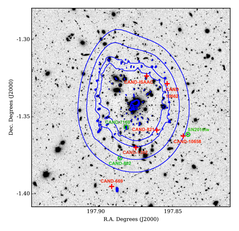
Figure 1: Near-infrared VLT/HAWK-I image of A1689 with critical lines for a source at $z_{s}$=2.0 plotted as contours for magnifications (from inside to outside) 2.0, 1.5, 1.0, and 0.75 magnitudes. The red crosses indicate the position of the core-collapse supernovae behind A1689 detected by our surveys, while the green circles denote those classified as Type Ia supernovae.

2.2 Near-infrared VLT/HAWK-I observations

The NIR data were obtained with the High Acuity Wide field K-band imager (HAWK-I; Pirard et al. 2004; Casali et al. 2006) mounted on the VLT (Programmes ID 082.A-0431, 0.83.A-0398, 090.A-0492, 091.A-0108, P.I. Goobar). The HAWK-I has an array of four $2048\times 2048$ HgCdTe detectors covering a total area of $7.5^{\prime}\times 7.5^{\prime}$ with a sampling of $0.106^{\prime\prime}/\rm{pix}$ per pixel. The chips are separated by a $15^{\prime\prime}$ gap.

The search was carried out in the J band, $1.17-1.34$ $\mu m$, with a pointing such that the galaxy cluster was placed in the centre of the field of view. The observations were executed in blocks of 29 exposures made of six 20 second integrations. Between each exposure, the telescope was offset in a semi-random manner. This allowed us to perform accurate sky subtraction and to fill in the gaps between the four arrays. The strategy was to execute two such blocks for each epoch, but when the observing constraints of $\leq 0.8\arcsec$ and photometric conditions could not be obtained for the full two hours during the same night, the observations for one epoch were spread over multiple nights. Nightly standard stars were also observed as part of the ESO standard calibration programme.

The J band data of A1689 were taken over 29 separate nights, starting on December 2008 and ending on July 2014, with an average seeing of $\sim$$0.6\arcsec$ (see Table 1 and Figure 2). The raw images were retrieved, immediately reduced and searched for transients as explained below. Additionally, a few epochs in $K_{s}$ band and the narrow NB1060 band were obtained by other programmes (ID: 085.A-0909, PI: D. Watson and ID: 181.A-0485, PI: J. G. Cuby) that observed the cluster during the same period.

2.3 Near-IR data reduction

The reduction of the VLT/HAWK-I data was carried out using a pipeline that includes procedures both from ESO and written by our group. The individual frames of each epoch were dark-subtracted and flat-fielded with the procedures from ESO Common Pipeline Library. For each frame a bad pixel mask consisting of saturated and cosmic ray affected pixels was produced.

To account for the contamination from the bright and variable atmosphere, standard NIR sky-subtraction was performed. For each exposure, the sky level in each pixel was estimated as the running median using the seven preceding and seven succeeding exposures after rejecting the three highest and lowest pixel values in the stack. In addition to these, we used an object mask to exclude any pixel that contained light from stars and galaxies. Contrary to the standard two-step NIR image reduction, the object mask was not created using the images obtained during the same night. Instead, we used the full set of images from the programme to create one deep image stack and built the object mask using SExtractor (Bertin & Arnouts 1996). This deep stack was continuously updated during the programme as new data were obtained.

We performed aperture photometry of isolated stars in the field for each night that also had standard star observations. From this we created a catalogue of the average stellar magnitudes. After excluding outliers, it was used as a tertiary standard star catalogue, as described below.

The individual frames were corrected for geometrical distortions by applying the distortion map provided by ESO. The distortion-corrected and sky-subtracted frames were then geometrically aligned and combined using SExtractor, SCAMP (Bertin 2006), and Swarp (Bertin et al. 2002). The frames from the four arrays were combined into a mosaic image (dubbed new image). For the transient search purpose (presented in Sect. 3, we split the list of frames into two parts and combined them for two more search images (new1 and new2). The mosaic images allowed us to search for transients between the chips, since large enough dithering steps were used to fill the gaps. However, the combined images were slightly shallower in these areas. Given that the core of the cluster was placed in the centre, many of the strongly lensed galaxies were located in these regions. It was a compromise to have the same pointing as archival data of the field.

To perform image differencing we used the software described in Fabbro (2001); Astier et al. (2006); Amanullah et al. (2008), which is based on the image subtraction algorithm from Alard & Lupton (1998) and Alard (2000). As a reference image (ref) in the subtraction process, we used either a single epoch or a deeper stack of several epochs that were significantly separated from the search epoch. The reference image was subtracted from new, new1, and new2 to create sub, sub1, and sub2, respectively.

Table 1: A1689 observations with VLT/HAWK-I in the J band

Date	Exp. time	Seeing	Det. eff.	$m_{lim}$
			90%	average
	(sec)	(arcsec)	(mag)	(mag)
2008-12-30	3420	0.69
2008-12-31	2400	0.57
2009-01-02	2400	0.65	23.05	22.97
2009-01-30	7200	0.61	23.63	23.54
2009-03-01	4800	0.53	23.85	23.67
2009-03-23	4800	0.62	24.15	24.44
2009-03-25	4800	0.38
2009-04-27	7200	0.56	23.87	23.87
2009-06-07	2400	0.66	23.28	23.10
2009-07-03	2400	0.61
2009-07-05	2400	0.63	23.53	23.49
2009-07-07	2400	0.73
2011-05-29	2400	0.87	Used as	24.30
2011-05-30	7200	0.44	a reference
2013-03-14	6960	0.61	23.92	24.11
2013-03-29	3480	0.44
2013-03-31	3480	0.57	24.26	24.44
2013-04-02	3480	0.36
2013-04-25	3480	0.61
2013-05-06	3480	0.44	24.19	24.69
2013-05-07	3480	0.44
2013-06-04	3480	0.64	23.48	23.97
2013-06-05	3480	0.61
2014-03-08	3480	0.48	23.95	23.62
2014-03-15	2160	0.59
2014-05-17	3480	0.82	23.52	23.28
2014-05-19	3480	0.91
2014-06-19	3480	0.78	22.55	22.77
2014-07-20	3480	0.37	23.94	23.74
Notes. The line indicates that a stack of those observations
was made.

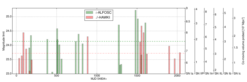
Figure 2: Magnitude limit for the HAWK-I and ALFOSC observations as presented in Tables 1 and 2. The red (green) dotted line indicates the average magnitude limit for the HAWK-I (ALFOSC) survey. On the right y-axis the probed co-moving volume in the J band is shown for each supernova type.

2.4 Optical NOT/ALFOSC survey

Adjacent to the NIR survey, we performed a complementary optical survey at the Nordic Optical Telescope (NOT; programmes P39-011, P46-008, P47-014, PI: A. Goobar). The NOT is a 2.56 m telescope at the Observatorio del Roque de los Muchachos at La Palma in the Canary Islands. We used the Andalucia Faint Object Spectrograph and Camera (ALFOSC), a $2048\times 2048$ pixel CCD with a field of view of $6.4^{\prime}\times 6.4^{\prime}$ and pixel scale of $0.19^{\prime\prime}/\rm{pix}$. We monitored A1689 in the $i$ band and searched for transients. We obtained additional data in the $g$ and $r$ bands. The images were centred on the galaxy cluster and a 9 point dithering pattern with the integration times listed in Table 2 was used.

The reduction of the optical images was carried out following standard IRAF procedures. The transient search was carried out using the method described above for the NIR data. The catalogue of tertiary standards with NIR photometry mentioned above was extended with the corresponding $gri$ magnitudes measured by the Sloan Digital Sky Survey.

Table 2: A1689 data from NOT/ALFOSC in the $i$ band searched for transients

Date	Exp. time	Seeing	Det. eff.	$m_{lim}$
			90%
	(sec)	(arcsec)	(mag)	(mag)
2009-06-05	3600	0.56	23.41	23.87
2009-06-24	3600	0.69	23.64	24.3
2010-01-15	3600	0.94	23.22	24.07
2010-03-17	3600	1.04	22.38	23.02
2010-05-17	3600	0.69	23.86	24.54
2010-05-21	3600	0.88	23.16	24.16
2010-06-12	3600	1.05	22.95	23.97
2010-07-11	3600	1.01	22.71	23.48
2011-01-02	3600	0.72	23.61	24.10
2011-02-06	3600	0.68	Ref
2011-03-29	3600	1.07	23.59	24.01
2012-05-14	3600	1.37	22.34	22.80
2012-06-21	3600	0.81	24.14	24.67
2012-07-06	3600	0.79	22.41	23.27
2012-07-22	3600	0.83	22.64	23.29
2013-01-15	3600	0.72	23.76	25.18
2013-02-11	3600	0.90	23.71	24.89
2013-03-28	3600	0.99	22.14	23.62
2013-05-17	3600	0.80	23.46	24.75

3 Transient search

After the image differencing, we ran an automated SN candidate detection algorithm on the subtracted images. Our search criteria were a S/N $\geq 5$ detection in the sub image and for the candidate to be present in both sub1 and sub2 with S/N $\geq 4$. As a first step, all candidates were methodically scanned by eye and ranked. The information available for each candidate includes S/N (for stacks and sub-stacks), distance to the nearest galaxy and the relative increase in brightness. Candidates arising from image subtraction artifacts at the cores of bright galaxies were revealed by low increase in brightness and rejected. Point source-like candidates with high S/N and a small angular separation from the core of a galaxy could come from AGN and were saved for further investigation.

In order to identify possible SNe, a careful examination of the remaining candidates was needed. This included:

• The image and subtraction stamps from all our previous NIR and optical data were inspected. Light curves from aperture photometry on the subtractions of the archival data were built for the saved candidates and checked for previous activity.

• High resolution HST/ACS images of the cluster were examined. The HST/ACS images have higher spatial resolution and S/N (in principle diffraction limited) compared to ground images. For this reason, faint background galaxies are often only visible in the HST/ACS images in which the transient could arise. In the case when the photometric/spectroscopic redshift of the presumable host galaxy was known, it was used to estimate the absolute magnitude of the transient. The lensing magnification was also taken into account.

After the survey was completed we repeated the transient search with improved reference images for our J-band data. Observations that were obtained less than 14 days apart were co-added to obtain better image depth. We were left with 15 combined images in total, and as reference for image subtraction, we used a deep image from 2011. Since there is a gap of observations between late 2009 and 2013, the reference image should not contain light from any SNe present in the earlier epochs. We limited the search area to the region with lensing magnification, $\mu\geq 2$, for an object at $z_{s}=2$. We required at least two consecutive detections and lowered the detection threshold to S/N$>4$. The initial number of candidates was $\sim$$10000$ (number of objects detected by the detection algorithm), of which with $\displaystyle\sim$$2/3$ were in the magnified region. We required less than five pixel separation to be considered the same candidate appearing in the different subtraction epochs. Given that our data span over five years, we rejected candidates that appeared in all the epochs, since we do not expect a significant fraction of SNe to be visible for such a long time in the band and redshifts considered here. In that way we discarded repetitive subtraction residuals. After the candidates ordering by their occurrence and the cuts applying, 184 candidates remained. Most of the candidates were subtraction residuals, arising from several reasons such as imperfect alignment between the new and the ref, or imperfect matching of the PSF of these two images. To be able to find real SN candidates, members of our team (TP, RA, and AG) visually inspected each of these remaining 184 candidates as described previously for the on-the-fly search. The candidates were ranked independently and the results were compared afterwards. Spurious detections appearing as candidates because of repetitive residuals on the same locations were rejected by all the inspectors. After the visual inspection, there were ten candidates that were rated highly. To exclude AGNs, we check the following: $i$) known AGN at the position of this transient and the galaxy, $ii$) galaxy activity in the previous epochs, and $iii$) that the transient is not located in the centre of the galaxy and cross-match the position to the X-ray point source catalogue . Two of the candidates were classified as AGNs.

3.1 Results

The transient search yielded a detection of eight SN candidates, six behind A1689, and two associated with cluster members, which are presented in Sect. 3.2 and 3.3 and summarized in Table 3. The transients were photometrically typed with a prior of the host galaxy redshift (spectroscopic or photometric). The only exception was CAND-1208 (SN 2010lw) for which a spectrum was obtained.

Table 3: Supernovae found in our VLT/HAWK-I+NOT/ALFOSC+VLT/ISAAC surveys.

SN ID	RA	DEC	Type	$z$	Redshift info	Magnification
CAND-1208	197.83987	-1.36145	Ia	0.189	SN spectrum	-
CAND-802	197.88393	-1.37678	Ia	0.214	Host spectrum	-
CAND-7169	197.88005	-1.35668	Ia	0.196	Host spectrum	-
CAND-ISAAC	197.86670	-1.32360	IIP	0.637	Host spectrum	$1.4\pm 0.07$
CAND-669	197.88937	-1.39524	IIL	0.671	Host spectrum	$0.31\pm 0.04$
CAND-821	197.86011	-1.35867	IIn	1.703	Host spectrum	$1.58\pm 0.07$
CAND-1392	197.87369	-1.37000	IIP	0.944	Host spectrum	$1.09\pm 0.07$
CAND-10658	197.84296	-1.36251	IIn	$z=0.94^{+0.07}_{-0.27}$	Host photo-$z$	$0.58\pm 0.06$
CAND-10662	197.85341	-1.32859	IIP	$z=1.03^{+0.20}_{-0.17}$	Host photo-$z$	$1.04\pm 0.07$

The brightness of each transient was measured using PSF photometry, where the flux for each epoch was fitted simultaneously together with a host-galaxy model and the transient position as described in, for example, Amanullah et al. (2008), Sect 3.1. The transient fluxes were then calibrated to the tertiary standards mentioned in Sect. 2.3.

We matched the coordinates of the candidate with our galaxy catalogues to determine the redshift of the SN host galaxies. When the redshift of the candidate host galaxy was not available, we used deep multi-band images from our survey and the template-fitting hyperz code (Bolzonella et al. 2000) to obtain the photometric redshift.

For the SN typing we used the light curve templates used in G09 that are also listed in Table 4. The templates were tested against the observed data for a grid of redshifts around the host $z$ and its $1\sigma$ confidence limits. The synthetic light curves in the observer NIR filters for redshift $z$ were obtained by applying cross-filter $k$-corrections, distance modulus, and time dilation corrections. There is also the possibility to have different reddening parameters ($E(B-V)$ and $R_{V}$). When we estimated the absolute V band magnitude $M_{V}$, we took the lensing magnification from the galaxy cluster into consideration.

The typing is not solely based on the best all-band $\chi^{2}$ fit, but on the best match to the fit parameters: the host redshift, the SN peak absolute magnitude, and the duration of the transient. The stamps, the multi-band photometry, and the best-fitted SN type light curves are shown in Figures 3 and 4 for the CC and SNe Ia, respectively.

Table 4: Supernova properties.

SN Type	$M_{V}\ (\rm mag)$	$\sigma_{M_{V}}\ (\rm mag)$	$f_{\rm CC}$
Ia	-19.30	0.30
IIP	$-16.90\pm 0.37$	0.97	0.524
IIL	$-17.98\pm 0.34$	0.90	0.073
IIn	$-18.62\pm 0.32$	1.48	0.064
Ib	$-17.54\pm 0.33$	0.94	0.069
Ic	$-16.67\pm 0.40$	1.04	0.176
faint CC SNe	$<15$		0.094
Notes. Second and third column indicate the peak V band
brightness $M_{V}$ and its one-standard-deviation $\sigma_{M_{V}}$, respecti-
vely. The third column stems for the fractions of core-colla-
pse supernova subtypes. Values adopted from
Richardson et al. (2014) and Li et al. (2011).

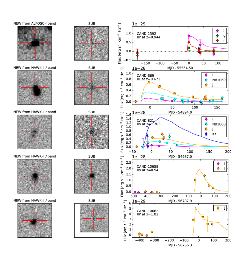
Figure 3: High-$z$ core-collapse supernovae behind A1689. The first two columns show $5\arcsec\times 5\arcsec$ image and subtraction stamps from epoch closest to maximum brightness. The location of the supernova candidates are indicated by the red markers. The third column contains the light curves of the supernova presented in the order as in the text: CAND-1392, CAND-669, CAND-821, CAND-10658 and CAND-10662. The solid lines represent the best-fitted SN template which are IIP, IIL IIn, IIn and IIP for the five SNe, respectively.

3.2 Core-collapse supernovae behind A1689

CAND-01392: The transient was discovered on 2011-01-02 in the three optical ALFOSC bands, but no NIR epochs were obtained while it was active. The most probable host for this transient is a galaxy that is centred $0\aas@@fstack{\prime\prime}32$ from the transient. The spectroscopic redshift of the host galaxy is $z=0.944$. At this redshift, the candidate is at a projected distance of $\sim$$3$ kpc from the host galaxy centre and the estimated magnification from the galaxy cluster is $1.09\pm 0.07$ mag. The transient is most likely a CC SN, where the best fit is a Type IIP SN with an absolute magnitude $M_{V}=-18.2\pm 0.13$, which differs by $1.3\sigma$ from the mean peak brightness of this class. The light curve is also consistent as the fading part of a SN IIn.

CAND-0669: The transient was found in the J band on 2009-03-01, and then observed later in the NB1060 and $i$ bands. The core of the most probable host is located $0\aas@@fstack{\prime\prime}49$ from the transient. The spectroscopic redshift of the galaxy is $z=0.671$, which means that the projected separation corresponds to $\sim$$3.5$ kpc. The magnification from the galaxy cluster is $0.31\pm 0.04$ mag. The best fit was obtained for the bright SN IIL with an absolute magnitude $M_{V}=-18.87\pm 0.07$. It is also possible, given the absolute magnitude, that the transient is a SN IIn. The absolute magnitude is also consistent with a SN Ia, however, taking into account the brightness in the NB1060 band and the lack of the second maximum in the observed J band, which corresponds to the rest-frame I band, a thermonuclear SN can be excluded (see e.g. Nobili et al. 2005).

CAND-0821: Our most distant transient was detected on 2009-06-05 in the $i$ band and confirmed a few days later in the J band. The SN has already been published in Amanullah et al. (2011a). An accurate galaxy host redshift $z=1.703$ was determined from a VLT/X-SHOOTER spectrum taken almost a year later, making CAND-821 one of the most distant CC SNe ever discovered. The SN is located $\sim 7$ kpc from the host galaxy centre. The SN has a significant lensing magnification of $1.58\pm 0.07$ mag. The best fit for this transient is a SN IIn with $M_{V}=-19.56\pm 0.06$. The detection in the rest-frame UV (observers $i$ band) excludes a thermonuclear SN. Further details are presented in Amanullah et al. (2011a).

CAND-10658: This SN candidate was found in the NIR epochs from 2014 in the post-survey search. The transient is located $0\aas@@fstack{\prime\prime}38$ from the core of a galaxy for which we estimated the photometric redshift to be $z=0.94^{+0.07}_{-0.27}$. At this redshift, projected host galaxy separation corresponds to $\sim 3$ kpc. The lensing magnification from the galaxy cluster is $0.58\pm 0.06$ mag for the given redshift. The light curve is consistent with a SN IIn with an absolute V band magnitude of $M_{V}=-22.00\pm 0.15$. SNe IIn with this intrinsic brightness have been observed (Smith et al. 2009; Chatzopoulos et al. 2011), and recent discoveries confirm that the SNe IIn class consists of objects that show the largest dispersion in peak magnitudes up to $M_{R}=-22.3$ (Anderson et al. 2014; Taddia et al. 2013; Richardson et al. 2014). The absolute magnitudes are usually reported in the $r/R$ band since most SNe IIn have the best coverage in the red bands. The rapid colour evolution of SNe IIn makes the conversion to V band less straightforward (Taddia et al. 2013). However, studies on individual SNe IIn suggest a (V-R) colour index of $0.05\pm 0.11$ at post-max epochs and $0.46\pm 0.05$ around maximum (Fassia et al. 2000; Di Carlo et al. 2002). In conclusion, the absolute magnitude of the candidate is compatible with SN IIn, thus the most probable classification for the transient is a SN IIn in the superluminous domain.

CAND-10662: As CAND-10658, this transient was found in the NIR epochs from 2014 in the post-survey search. The S/N $<5$ so it would not have been detected on the fly. The most likely host galaxy has a photometric redshift of $z=1.03^{+0.20}_{-0.17}$ and is located $0\aas@@fstack{\prime\prime}27$ from the transient. With the given redshift the magnification from A1689 at this position is $1.04\pm 0.07$ mag and the projected separation corresponds to $\sim$$2.2$ kpc. The best light curve fit was obtained for a SN IIP with $M_{V}=-17.46\pm 0.21$.

CAND-ISAAC: This transient was detected in the ISAAC pilot survey and typed as a SN IIP at a photometric redshift of $z=0.59\pm 0.05$ in G09. A spectrum of the host galaxy was published later (Frye et al. 2012) placing it at $z=0.637$, which is consistent with the initial estimate.

3.3 Type Ia supernovae in and behind A1689

Three SNe Ia were found in the survey, of which two were found be associated with host galaxies that belong to A1689. The host galaxies are shown in the first column of Figure 4. The observed light curves were used to classify the SNe using the method described in 3.1. Given this, we further use the SNooPy package (Burns et al. 2011) to fit light curve parameters, such as the date of B band maximum, $t_{\mathrm{max}}$, the brightness decline between peak and day $+15$ of the rest-frame B-band light curve, $\Delta m_{15}$, the host galaxy extinction , $E(B-V)_{\mathrm{host}}$, and the distance modulus, $\mu$. This process involves extrapolation from the multi-band observed photometry. In order to fit $\mu$, SNooPy takes advantage of the fact that normal SNe Ia are a very homogeneous class of objects with a narrow distribution of absolute magnitudes. The SNooPy package includes optical to NIR SN Ia light curve templates based on a SN Ia sample obtained by the Carnegie Supernova Project. The spectral energy density template from Hsiao et al. (2007) is used for calculating cross-filter k corrections.

The best-fit light curve parameters for the three SNe Ia are presented in Table 5, and the corresponding light curves are shown in Figure 4 together with the measured data. In the last column of the table, we present the distance moduli calculated from the redshifts, assuming a flat Universe with $H_{0}=72\,$km/s/Mpc and $\Omega_{\rm M}=0.28$, which are the values used for the calibration of SNooPy. Details of the individual transients are given below.

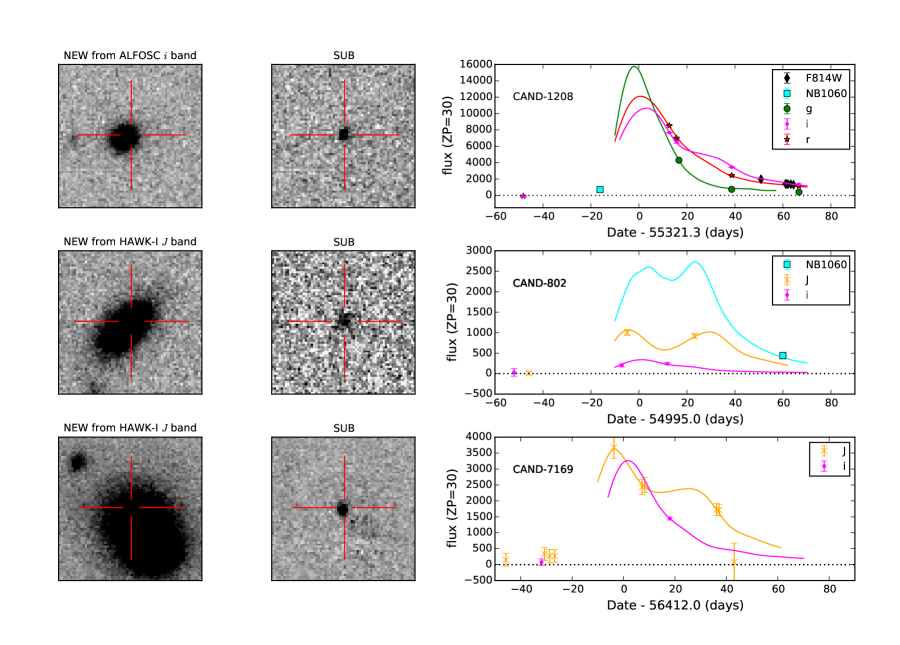
Figure 4: Supernovae Type Ia found in the surveys. The first two columns show 7$\arcsec\times 7\arcsec$ stamps from the epochs (image and subtraction image) closest to maximum brightness of the transient. The location of the supernova candidate is indicated by the red markers. The third column contains the light curves of the SNe presented in the order as in the text: CAND-1208, CAND-802 and CAND-7169.

Table 5: Fitted light curve parameters obtained with SNooPy . The redshifts were adopted from Table 3, and the distance moduli in the last column were calculated from the redshift assuming a flat Universe with $H_{0}=72\,$km/s/Mpc and $\Omega_{M}=0.28$.

SN		$z$	$t_{\mathrm{max}}$	$\Delta m_{15}$	$E(B-V)_{\mathrm{host}}$	$\mu$	$\mu_{\mathrm{cosmo}}$
			(days)	(mag)	(mag)	(mag)	(mag)
$1208$	a	$0.189$	$55321.3(0.4)$	$0.67(0.02)$	$0.06(0.02)$	$39.34(0.03)$	39.76
$802$		$0.214$	$54995.0(4.5)$	$1.57(0.27)$	$2.12(0.80)$	$40.97(0.42)$	40.06
$7169$		$0.197$	$56412.0(1.6)$	$1.67(0.01)$	$0.39(0.07)$	$39.66(0.05)$	39.86
a SN 2010lw

CAND-01208 (SN 2010lw): The transient was discovered with the NOT on 2010 May 17.944 UT in the $i$ band and also observed in the $g$ and $r$ bands (Amanullah et al. 2011b). It was located $0\aas@@fstack{\prime\prime}77$ west and $0\aas@@fstack{\prime\prime}35$ north of its host galaxy, which is a member of A1689 at redshift $z=0.189$. A spectrum of the candidate was obtained with NOT/ALFOSC on 2010-05-21.9 UT, using Grism 4 and a $1.3\arcsec$ slit. The spectrum was reduced using standard IRAF routines. Using SNID (Blondin & Tonry 2007), we found several good matches to normal SNe Ia at +16 ($\pm 8$) days after maximum brightness (see Figure 5 for a comparison between SN 2010lw and the normal SN Ia 2005hf). SNID also provides good matches to over-luminous 91T-like SNe and the peculiar SN 2007if (Scalzo et al. 2010), which are also consistent with the parameters derived from the light curve fits.

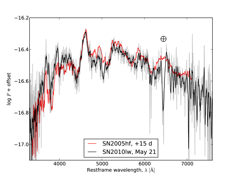
Figure 5: Spectrum of SN 2010lw (CAND-01208) obtained with ALFOSC at the NOT (black line). The Earth symbol indicates a strong telluric feature that is not corrected for. The red line shows a spectrum of the normal SN Ia 2005hf at 15 days past maximum brightness.

CAND-0802: The transient was discovered on 2009-06-07 in the J band and later observed in the $i$ band and the NB1060 band. The SN is located $4\aas@@fstack{\prime\prime}1$ from the nucleus of the host galaxy at a spectroscopic redshift of $z=0.214$ (Martini et al. 2007). Even though the galaxy is located close to the cluster core region in projection space, most likely this galaxy does not belong to A1689. A1689 member galaxies have a relatively wide internal velocity spread and they extend to large radii (Lemze et al. 2009). Moreover, there is evidence that there are two groups of galaxies merging (Czoske 2004). Velocity offsets from the mean cluster redshift are defined as $v=c(z_{galaxy}-z_{cluster})/(1+z_{cluster})$ (Harrison & Noonan 1979). The redshift difference for this host galaxy is significant and it would require a velocity offset of $6300$ km s^-1. Lemze et al. (2009) find maximum amplitude of $\mid$$4000$$\mid$ km s^-1, which places this SN host behind the cluster and not in it.

The best-fit light curve parameters suggest a significant host reddening, which is rarely found in transient searches at bluer wavelengths, and a steep decline rate. The low-resolution spectrum of the host galaxy shows strong emission lines that indicate ongoing star formation. The presence of dust is usual for these environments. Given the high reddening, the best-fitted distance modulus could be slightly biased by the assumption of the total-to-selective extinction, but despite this we note that the distance modulus is within $\sim 2\sigma$ of the expected value based on the redshift.

CAND-7169: The transient was discovered on 2013-05-06 in the J band and later observed in the $i$ band. The host is an elliptical galaxy with spectroscopic redshift $z=0.1958$. The SN was located $1\aas@@fstack{\prime\prime}42$ from the core of its host galaxy. The SNooPy fit results suggests a rapidly declining, reddened SN.

3.4 Discussion

We compare our results to the expected number of events and their redshift distribution using existing rate models applied to our survey.

We estimated the expected number of CC SNe by following the same procedure as in G09. We used CC SN rate as extrapolated in G09 and based on the results in Mannucci et al. (2007). The control times are calculated in the same way as for the volumetric rates estimation presented in the next sections. We assumed moderate overall reddening in the host galaxies with $E(B-V)=0.15$ and Milky Way-like extinction law $R_{V}=3.1$ (Cardelli et al. 1989).

The result is shown in Figure 6 and indicates that our survey was sensitive up to $z\approx 2$ for most SN subtypes and even to $z\approx 3$ for the brightest CC SNe. Moreover, the most expected subtypes were SNe IIP around $z\approx 0.5-1$ and SNe IIn at $z\approx 0.8-1.2$, thus reflecting the types and redshift distribution of our discoveries well.

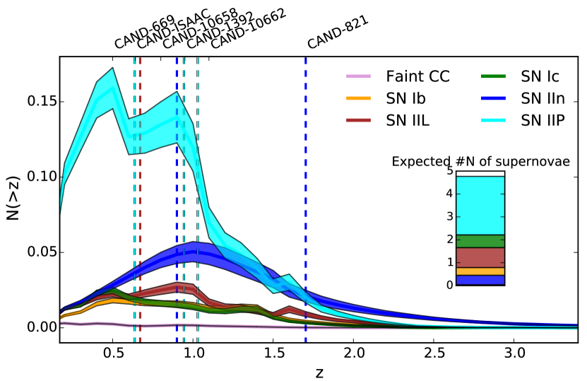
Figure 6: Redshift distribution of core-collapse supernova discoveries expected from the surveys with a rate model from Mannucci et al. (2007). The redshift of the core-collapse supernova candidates from our surveys are indicated with dashed line. The total expected number of core-collapse supernovae is also shown.

Next, we investigate the consistency of detecting a single SN Ia outside A1689 with the expectations. We ran a similar simulation considering three SN Ia rate models based on the rates from the Supernova Legacy Survey (SNLS; Neill et al. 2006), the so-called ”A+B model” from Scannapieco & Bildsten (2005), and the best fit to the GOODS rates (Dahlen et al. 2008, 2012) corresponding to a delay time $\tau=1.0$ Gyr. This delay time refers to the time between star formation and the SN Ia explosion and was assumed to follow a Gaussian distribution. The integrated number of SN Ia events are $2.2$, $3.7$, and $1.7$, respectively. We conclude that the detection of a single event is consistent with expectations.

4 Volumetric SN rates

Next, we calculate the volumetric SN rates. The volumetric SN rate, $r_{V}^{j}$, for a SN type $j$ (in units Mpc^-3yr$\leavevmode\nobreak\ {}^{-1}h^{3}_{70}$) is given by

$$r_{V}^{j}(z)=\frac{N_{j}(z)}{T_{j}(z)\cdotp V_{C}(z)}(1+z),$$ (1)

where $T_{j}(z)$ is the visibility time (often called the survey control time), which indicates the amount of time the survey is sensitive to detecting a SN candidate (Zwicky 1938). The value $N_{j}$ is the number of SNe and $V_{C}$ is the co-moving volume. The factor $(1+z)$ corrects for the cosmological time dilation. The number of observed SNe, $N_{\rm raw}$, was corrected for the redshift migration effect to obtain the real debiased number, $N_{\rm debiased}$ (see Sect. 4.2). We calculated the volumetric rates for the search area as defined in the post-survey search, so we only considered the SNe inside this field (see Figure 1).

The monitoring time above the detection threshold for a SN of type $j$, $T_{j}$, is a function of the SN light curve, absolute intrinsic SN brightness, $M$, detection efficiency (see Appendix A), $\epsilon$, extinction by dust, $\Delta m_{\rm ext}$, and the lensing magnification, $\Delta m_{lens}$. The probability distributions of the absolute intrinsic brightness $P(M)$ are assumed to be Gaussian with properties listed in Table 4. Following a similar procedure as in G09, the control time is obtained as

$$\begin{split}T_{j}(z,\Delta m_{\rm ext}+\Delta m_{\rm lens})=\\ =\int{\epsilon(m){P(M)}\Delta t_{j}(z,M+\Delta m_{\rm ext}+\Delta m_{\rm lens})dM},\end{split}$$ (2)

where $\Delta t_{j}$ is the time period when the SN light curve is above the detection threshold. We combined the control time of the NIR and optical surveys and included the VLT/ISAAC survey from G09.

We calculated the control time for SNe Ia and CC separately. The control time depends on the properties of the light curves, so different subtypes of CC SNe have different control times. The total CC control time was obtained by weighting the contribution from the various CC SN subtypes with their fractions (shown in Table 4) and then summed.

The volumetric rates were measured in redshift bins chosen to match other surveys for easier comparison. There are five redshift bins in the range $0.4\leq z<2.9$ with equal bin width of $\Delta z=0.5$. We start at $z=0.4$ and postpone the discussion of the cluster rate to Sect. 7. We placed the measurements of the rates at the effective redshift of each bin, where the weighting is done with the control time.

The co-moving volume, $V_{C}$, contained in the redshift bin between $z_{1}<z<z_{2}$ was computed as

$$V_{C}=\int\limits_{z1}^{z2}\frac{c\cdotp d_{L}^{2}(z)}{H(z)\cdotp(1+z)^{2}}\omega\cdotp dz,$$ (3)

where $d_{L}$ is the luminosity distance, $c$ is the speed of light in vacuum, $H(z)$ is the Hubble parameter at redshift $z$ in units of $\rm km\cdotp s^{-1}Mpc^{-1}$, and $\omega$ denotes the solid angle, corrected by the lensing magnification $\mu$. The spatial variation of the magnification is accounted for by integrating over the field of view when calculating $\omega$ (see G09 for details). Figure 2 shows the J band survey volume summed in the line of sight for each SN type. Given that the J band is more sensitive to high-$z$ SNe, the corresponding volume for the $i$ band survey is between $\sim 1.4$ and $\sim 2.1$ times smaller, depending on SN type.

Observations of SNe are likely to suffer from extinction in the host galaxy, which influences the rate estimate. Making an appropriate correction to account for this is very important, however, this correction represents one of the most uncertain assumptions in the rates analysis. We assumed a Milky Way-like extinction law (Cardelli et al. 1989) with $R_{V}=3.1$ for both SN Ia and CC SN rates. In Sect. 4.2 we compare this assumption to the impact of using a starburst extinction law with $R_{V}=4.05$ (Calzetti et al. 2000) for CC SNe.

The values for the colour excess were drawn from a positive Gaussian distribution with a mean $E(B-V)=0.15$ and $\sigma_{E(B-V)}=0.02$ similar to Dahlen et al. (2012). Our choice of extinction correction is further justified by Alavi et al. (2014), who studied $z$$\sim$$2$ galaxies behind A1689 and found an average reddening $E(B-V)=0.15$ mag.

Extinction corrections for SN rates were studied in Hatano et al. (1998) and Riello & Patat (2005) with MCMC predictions that depend on several assumed parameters of the SN, host galaxy, and dust properties. Dahlen et al. (2012) and Mattila et al. (2012) compiled observed extinction properties of nearby CC SN sample with mean extinction $A_{V}=0.42\pm 0.09$ mag. This is very close to the predicted mean value $A_{V}=0.44$ derived from a distribution of expected $A_{V}$ values from the model in Riello & Patat (2005). It is difficult to measure $A_{V}$ directly for individual CC SNe at higher $z$; we can only detect those with low $A_{V}$ and there is a relatively large spread of their absolute magnitudes. Since a detailed understanding of the evolution of the dust content in galaxies with redshift is still lacking, we follow previous work (Melinder et al. 2012; Graur et al. 2011; Strolger et al. 2015) and assume equal reddening over our entire redshift range.

To calculate the upper limits for SN Ia rates, we used the high extinction dust model from Rodney et al. (2014), where $A_{V}$ follows a Gaussian distribution with $\mu=0.5$ and $\sigma=0.62$.

4.1 Results

Thanks to the magnification from A1689, our search was sensitive to high-redshift SNe (see Figure 6). We present measurements and pose upper limits on the SN rates in five redshift bins from $0.4\leavevmode\nobreak\ \leq\leavevmode\nobreak\ z\leavevmode\nobreak\ <\leavevmode\nobreak\ 2.9$. Since we did not detect any confirmed SN Ia behind the galaxy cluster in these redshift bins and our survey was sensitive to these events, we only present the limits.

Our rates are summarized in Table 6 and shown in Figure 7. For comparison, in the same figure we also plot measurements from other authors. At lower redshifts we include measurements from Botticella et al. (2012); Mattila et al. (2012); Li et al. (2011); Cappellaro et al. (1999); Taylor et al. (2014); Graur et al. (2015); Bazin et al. (2009); Botticella et al. (2008); Cappellaro et al. (2015). At the higher redshifts range, ($z\gtrsim 0.4$), fewer results exists; these are Subaru Deep Field (SDF) at $\langle z\rangle=0.66$ (Graur et al. 2011), the Stockholm VIMOS Supernova Survey (SVISS) at $\langle z\rangle=0.39$ and $\langle z\rangle=0.73$ (Melinder et al. 2012), and the combined rates from GOODS+CANDELS+CLASH survey at $\langle z\rangle=0.3$, $\langle z\rangle=0.7$, $\langle z\rangle=1.5$, $\langle z\rangle=1.9$ and $\langle z\rangle=2.3$ (Dahlen et al. 2004, 2012; Strolger et al. 2015).

Our rate measurements are slightly higher than the results from all other surveys at $\langle z\rangle=1.06$ and $\langle z\rangle=1.57$, but our rate measurements are consistent with all other measurements when taking statistical and systematic errors into account. We also plot the predictions from different star formation histories which we discuss in Sect. 5.

Table 6: Field SN numbers and volumetric rates

Redshift bin	$0.4\leq z<0.9$	$0.9\leq z<1.4$	$1.4\leq z<1.9$	$1.9\leq z<2.4$	$2.4\leq z<2.9$
Effective redshift	0.57	1.06	1.57	2.06	2.56
$\rm N_{\rm CC}$(raw)	1	3	1	0	0
$\rm N_{\rm CC}$(debiased)	1.51	2.48	1.01	0	0
$r_{\rm V,CC}$ (no ext.)a,b	$\displaystyle 2.6^{+4.2}_{1.8}\displaystyle$	$8.7^{+9.8}_{-5.2}$	$8.1^{+18.5}_{-6.7}$	$<57$	$<251$
$r_{\rm V,CC}$ (norm.ext.)	$\displaystyle 2.8^{+4.5}_{-2.0}$	$10.3^{+11.5}_{-6.1}$	$10.8^{+24.4}_{-8.9}$	$<88$	$<398$
Effective redshift	0.61	1.09	1.59	2.07	2.54
$\rm N_{\rm Ia}$ (raw)	0	0	0	0	0
$r_{\rm V,Ia}$(no ext.)a	$<3.6$	$<2.7$	$<3.5$	$<5.8$	$<20.4$
$r_{\rm V,Ia}$(with high ext.)	$<3.8$	$<3.0$	$<4.5$	$<9.6$	$<62.1$
Notes. The volumetric supernova rates $r_{V}$ are given in [10-4 yr-1 Mpc${}^{-3}h^{3}_{70}$].
aThe errors, are the 68% Poisson statistical uncertainties of the number of SNe propagated to the rates.
bThe highest two redshift bins for the CC SN rates and all the SN Ia rates are upper limits with $2\sigma$ Poisson
uncertainty.

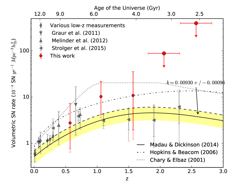
Figure 7: Measured core-collapse supernova rates with our NIR+optical (VLT/HAWK-I + NOT/ALFOSC) surveys presented here and VLT/ISAAC survey presented in Goobar et al. (2009). Core-collapse supernova rate measurements from the literature are also shown; we plot the results with normal host galaxy extinction. Error bars are statistical with total errors (statistical and systematic added in quadrature) as a transparent/faded extra error bar for all surveys. The various lines represent cosmic star formation histories from several authors scaled with $k_{8}^{50}=0.007$. The best-fitted value to the rates data of the scale factor $k_{\rm CC}=0.00930\pm 0.00096$ is also shown.

4.2 Sources of uncertainties in the CC SN rates

Our error budget is dominated by the Poisson uncertainties from the low number of events in our survey. To assess the impact of the many assumptions we made, we estimate of the systematics errors in detail and discuss them below. The resulting systematic uncertainties per redshift bin are summarized in Table 7 along with the statistical uncertainties for comparison. In order to quantify the contribution to the systematic uncertainties of the rate calculation, we re-calculated the control time with several assumptions and derived the volumetric rate. The uncertainties in the detection efficiency function are small in comparison with the sources of error. Since we only provide upper limits for SNe Ia rates at redshift bins where there are ample existing measurements (see e.g. Rodney et al. 2014, for a recent volumetric SN Ia rate compilation), we did not engage in detailed estimation of the systematic uncertainties.

Mis-typing: Incorrectly classified candidates as CC SNe instead of SN Ia or AGN, introduces an error in the rates. For this reason, we discuss the SN typing thoroughly in Sect.  3.2. As an attempt to quantify the possible systematic offset caused by misclassification, we excluded one of the SNe in the rate calculation at $z=0.94$. In this way, we obtained lower rates of $\sim$$20\%$ and $\sim$$30\%$ at $\langle z\rangle=0.57$ and $\langle z\rangle=1.06$, respectively which is smaller than the statistical uncertainty.

Redshift migration: Uncertainty in the SN redshift introduces uncertainty in the rate determination. Using Monte Carlo simulations we redistributed the SNe with a Gaussian distribution where the mean and standard deviations are the SN redshift and its error, respectively. The derived errors are then propagated into the SN rates.

The effect of the redshift migration can have a significant contribution on the systematics if the SN typing only relies on the photometric redshift of the host galaxy. This highlights the importance of having a spectroscopic redshift measurement of the galaxy or, even better, spectroscopic confirmation of the SN candidate.

Host galaxy extinction: To estimate the extinction correction uncertainties in the CC SN rates, we tested several assumptions for the extinction parameters. Rodney et al. (2014) (lower panel of their Figure 7) show three dust models for CC SNe population based on observational evidence. The different distributions for $A_{V}$ are generated from the positive half of a Gaussian distribution centred at $A_{V}=0$ with dispersion $\sigma$, plus an exponential distribution of the form $e^{-A_{V}/\tau}$. Their low extinction model with $\sigma=0.15,\tau=0.5$ matches well with our assumption made for the rate calculation. Their high extinction model with $\sigma=0.8,\tau=2.8$ yields higher CC SN rates by $15\%$ at $\langle z\rangle=0.57$, $37\%$ at $\langle z\rangle=1.08$, and $72\%$ at $\langle z\rangle=1.57$.

We also calculated the rates with negligible extinction, $E(B-V)=0$ (also shown in Table 6). The CC SN rates decreased by $7\%$ at $\langle z\rangle=0.57$, $\langle z\rangle=1.08$, $16\%$ at $\langle z\rangle=1.08$, and $30\%$ at $\langle z\rangle=1.57$, which provides the extreme lower limit to the estimate.

Mannucci et al. (2007) and Mattila et al. (2012) showed that a large fraction of the SNe exploding in galaxies can be missed because of severe dust obscuration. In particular, this should happen in galaxies known as luminous IR galaxies (LIRGs) and ultra-luminous IR galaxies (ULIRGs), where most of the UV light is processed into thermal IR heating by dust. We used the correction factors to account for the missing SN fraction from Mattila et al. (2012) as an extreme upper limit to the uncertainty estimate of the host extinction correction. The resulting missing SN fractions weighted by our control time are $47\%$ at $\langle z\rangle=0.57$, $56\%$ at $\langle z\rangle=1.06$ and $58\%$ at $\langle z\rangle=1.57$. These correction factors are based on the observations of the nearby LIRG Arp 299 and the missing fraction of SNe in high-$z$ U/LIRGs remains uncertain. In particular the assumption that the properties of the U/LIRGs do not change significantly with time might not hold.

We also quantified the impact of the assumption regarding the extinction law for CC rates, by assuming attenuation law with $R_{V}=4.05$ that is appropriate for starburst galaxies (Calzetti et al. 2000).We found a small impact on our rates results; they become higher by $1\%$ at $\langle z\rangle=0.57$, $1\%$ at $\langle z\rangle=1.08$, and $2\%$ at $\langle z\rangle=1.57$.

CC SN fractions and peak magnitudes: Throughout the CC SN rates calculations, we have used the SN properties from the Asiago Supernova Catalogue (ASC) as compiled by Richardson et al. (2014) and the fraction of the CC SN subtypes from the Lick Observatory Supernova Search (LOSS) (Li et al. 2011). If we instead use the SN fractions and properties as compiled in Table 1 in G09 based on older ASC results (Richardson et al. 2002), we obtained lower rates, $\sim$$17\%$ at $\langle z\rangle=1.08$ and $\sim$$19\%$ at $\langle z\rangle=1.57$. However, the uncertainty in the relative fractions is large. For instance, in the newer estimate, Richardson et al. (2014) found a much lower fraction of Type IIL of 7.3% than the 20% in Richardson et al. (2002). Also, measured CC SN fractions are based on a nearby sample study and might not be representable at higher redshifts where CC SN fractions are quite unknown.

Unlike SNe Ia, CC SNe show large spread in the values of the mean peak absolute magnitudes. To estimate the effect on the rates, we propagated the standard error of the mean peak absolute magnitudes for each subtype of CC SNe (shown in Table 4, values taken from Richardson et al. (2014)). We obtained $-12/\!+\!14\%$ at $\langle z\rangle=0.57$, $-20/\!+\!23\%$ at $\langle z\rangle=1.08$, and $-25/\!+\!29\leavevmode\nobreak\ \%$ at $\langle z\rangle=1.57$.

Magnification maps: The uncertainties in the magnification maps of A1689 propagate to uncertainties of the estimated rates since they affect both the control time and the probed co-moving volume. A larger (smaller) magnification would result in an increased (decreased) control time, but at the same time a smaller (larger) volume is probed. The uncertainties originating from the magnification maps are insignificant at $\langle z\rangle=0.57$, $\pm 3\%$ at $\langle z\rangle=1.08$ and $-3/\!+\!1\%$ at $\langle z\rangle=1.57$.

Cosmic variance: We used a relatively small field of view around A1689 to measure SN rates, which can lead to uncertainty due to the local inhomogeneity. To account for this, we calculated our systematic errors coming from cosmic variance based on the recipe from Trenti & Stiavelli (2008) and assumed that the variances of the SNe follow the overall galaxy population. We estimate that the uncertainties are $\sim$$14\%$ at $\langle z\rangle=0.57$, $\sim$$15\%$ at $\langle z\rangle=1.08$, and $\sim$$17\%$ at $\langle z\rangle=1.57$.

Table 7: Relative systematic error budget

Error source	CC Supernovae
	$0.4\leq z<0.9$	$0.9\leq z<1.3$	$1.4\leq z<1.8$
Redshift migration	$\pm 0.68$	$\pm 1.74$	$\pm 0.11$
Subtype fractions	$\pm 0.09$	$\pm 1.38$	$\pm 2.35$
Peak magnitudes	$-0.32/+0.38$	$-2.01/+2.35$	$-2.78/+2.98$
Extinction law	$\pm 0.03$	$\pm 0.01$	$\pm 0.13$
Dust extinction	$-0.05/+0.04$	$-0.25/+0.35$	$-0.49/+0.48$
Extreme dust extinction limits	$-0.19/+1.21$	$-1.55/+4.90$	$-2.62/+4.73$
Magnification maps	$\pm 0.01$	$-0.28/+0.35$	$-0.37/+0.14$
Cosmic variance	$\pm 0.38$	$\pm 1.56$	$\pm 1.83$
Total systematic	$-0.76/+0.79$	$-3.01/+3.27$	$-3.70/+3.83$
Statistical	$-1.98/+4.51$	$-6.06/+11.48$	$-9.56/+26.36$

5 Core-collapse supernova rate and cosmic star formation history

Since CC SNe have massive and short-lived stars as progenitors, their rates, $r^{\rm CC}_{V}(z)$, should reflect the ongoing star formation rate $\psi(z)$ (SFR) with a simple relation,

$$r^{\rm CC}_{V}(z)=k_{\rm CC}\cdot\>h^{2}\cdot\psi(z),$$ (4)

where the scale factor $k_{\rm CC}$ is the number of stars per unit mass that explode as SNe. The constant is obtained as the ratio of the two integrals

$$k_{\rm CC}=\frac{\int_{M_{min}}^{M_{max}}{\phi(M)dM}}{\int_{0.1M_{\odot}}^{125M_{\odot}}{M\phi(M)dM}},$$ (5)

where $\phi(M)$ is the initial mass function (IMF), which is the empirical function that describes the mass distribution of a population of stars. We assumed that $k_{\rm CC}$ does not evolve with redshift. Similar to previous high-$z$ CC SN rate studies, we used a Salpeter (1955) IMF and $M_{min}=8\>\rm M_{\odot}$ and $M_{max}=50\>\rm M_{\odot}$ as range of stellar masses that explode as CC SNe. With these assumptions, the scale factor is $k_{8}^{50}=0.0070^{+0.0019}_{-0.0022}\>\rm M_{\odot}^{-1}$. The uncertainty comes from the assumed IMF and the extremes of integration i.e. the stellar mass ranges that end up as CC SNe (see e.g. Melinder et al. 2012; Cappellaro et al. 2015; Strolger et al. 2015, for a detailed discussion).

The estimate of the SFH is based on several SF tracers, which depend on the parametrization of the SF function and the applied dust extinction. In fact, only recently has a clear picture of the SFH emerged (Madau & Dickinson 2014) in which these authors found a consistent SFR density which peaks at $z\approx 1.9$ and then declines exponentially. By using a scale factor of $k_{\rm CC}=0.007$, Madau & Dickinson predicted CC SN rates that were in good agreement with the results in Dahlen et al. (2012). Before the revised version of cosmic SFH presented by Madau & Dickinson (2014), it was suspected that the cosmic CC SN rate did not match the massive SF rate and that the CC SN rate was lower by factor two (Horiuchi et al. 2011). From the overall CC SN rate available and the predictions from the Madau & Dickinson (2014) SFH, that problem is not evident anymore.

Instead of using the scale factor $k$ from a Salpeter IMF and the above-mentioned mass ranges, we can empirically obtain the value for $k$ by fitting the $\psi(z)$ to our CC rates and all available literature values. We used the weighted least-squares fit of the SFH parametrization from Madau & Dickinson (2014) as follows:

$$\psi(z)=A\,\frac{(1+z)^{C}}{1+((1+z)/B)^{D}}\quad[\rm M_{\odot}\,year^{-1}Mpc^{-3}]$$ (6)

with their best-fit values $A=0.015$, $B=2.9$, $C=2.7$, and $D=5.6$. We used the Levenberg-Marquardt least-squares algorithm and we obtained the best fit for $k_{\rm CC}=0.00930\pm 0.00096$, which is similar to what was found in Strolger et al. (2015). The result with its uncertainty is shown in Figure 7. This value is within $\sim$$1\sigma$ of $k_{8}^{50}$.

Strolger et al. (2015) attempted to predict the shape of $\psi(z)$ by using re-binned measured values in five redshift bins from the literature and the combined GOODS+CANDELS+CLASH surveys. We added our results and the newly published measurements at $\langle z\rangle=0.10$ and $\langle z\rangle=0.25$ from the Supernova Diversity and Rate Evolution survey (SUDARE; Cappellaro et al. 2015) to obtain new comprehensive weighted average rates in the same redshift bins. We obtained $A=0.016\pm 0.004$, $B=1.9\pm 0.7$, $C=4.3\pm 1.7$, and $D=6.2\pm 2.5$. However, in addition to the comparable number of points with the number of parameters, this procedure is sensitive to the choice of binning and anchoring low-$z$ point. In conclusion, a robust prediction of the SFH from the CC SN rate remains difficult at present.

6 Supernovae in the resolved strongly lensed multiply-imaged galaxies

Based on photometric studies on HST/ACS images, there are more than 100 multiple images of $40$ strongly lensed background galaxy sources with redshifts ranging from $z=1$ to $z=4.9$ behind A1689 (Broadhurst et al. 2005, Limousin et al. 2007, Diego et al. 2015). Our survey was sensitive to SNe that could have exploded in these galaxies. For example, the multiple images (labelled 1.1 and 1.2) of galaxy source 1 at $z$=3.04, are magnified by $3.80^{+0.30}_{-0.29}$ and $5.58^{+1.21}_{-0.74}$ mag, respectively (Riehm et al. 2011). With this magnification, most subtypes of SNe were detectable with our NIR survey. Furthermore, the time delay between these two images is $83^{+77}_{-69}$ days (Riehm et al. 2011), which is well within the total length of our programme. In other words, if a SN had exploded in this galaxy, the SN could have been detected in both 1.1 and 1.2 during the survey (see Figure 10).

Because of their standard candle nature, observations of SNe Ia through lensing clusters are particularly interesting. By estimating the absolute magnification of SNe Ia, it is possible to break the so-called mass-sheet degeneracy of gravitational lenses. Thus, they could be used to put constraints on the lensing potential, if the background cosmology is assumed to be known (see e.g. Nordin et al. 2014). This can be further improved by observations of strongly lensed SNe Ia, through the measurements of time delays between the multiple images. In contrast, if the lensing potential is well known instead, measurements of time delays of any transient source can be used to measure the Hubble constant and, to a lesser degree, the density of the cosmic fluids (Refsdal 1964; Holz 2001; Bolton & Burles 2003; Oguri & Kawano 2003; Oguri 2007; Zitrin et al. 2014; Riehm et al. 2011). At the high redshifts where these galaxies are located, the SN rates are dominated by CC SNe and the SN Ia rates are expected to be lower owing to the delay between the star formation and explosion.

Here, we calculate the expected number of SNe in the multiply lensed background galaxies from our NIR survey. As in Riehm et al. (2011), we only considered those that have a spectroscopic redshift and a predicted time delay of less than five years. There are 17 systems with 51 images that satisfy these criteria. These are shown in Figure 9. To obtain the expected number of SNe in each galaxy $N_{i}$, we multiply the SN rate $R_{i}$ and the control time $T_{i}$,

$$N_{i}=R_{i}\cdot T_{i},$$ (7)

where $i$ indicates the individual galaxies. To estimate the SN rate in each galaxy, we used the SFR estimated previously in Riehm et al. (2011) and G09, using the rest-frame UV luminosity at $2800\,\AA$ as a tracer. The expected CC SN rate for each galaxy in units yr^-1 was then calculated from

$$R_{\rm CC}=k_{8}^{50}\cdot SFR,$$ (8)

where the SFR is given in in units $[M_{\odot}$yr^-1]. The SN Ia rates were obtained from the Scannapieco & Bildsten (2005) two-component model

$$R_{Ia}=A\cdot SFR+B\cdot M_{*},$$ (9)

where the stellar mass $\rm M_{*}$ of the individual galaxies was obtained from the rest-frame B band luminosity via the relations from Bell et al. (2003). The total expected number of SNe over all the systems are then simply summed. The result is $N_{\rm CC}=0.23\pm 0.11$ and $N_{\rm Ia}=0.14\pm 0.09$ for CC SNe and SNe Ia, respectively. This means that the chance of detection a SN in the strongly lensed galaxies was rather low.

Since we have not detected any SN in these galaxies with multiply lensed images, we calculated the upper limit of the rates for both SNe Ia and CC. The control time of the galaxies belonging to the same system (indicated with the same first number in Figure 9) was summed. The result of this comparison is shown in Figure 8.

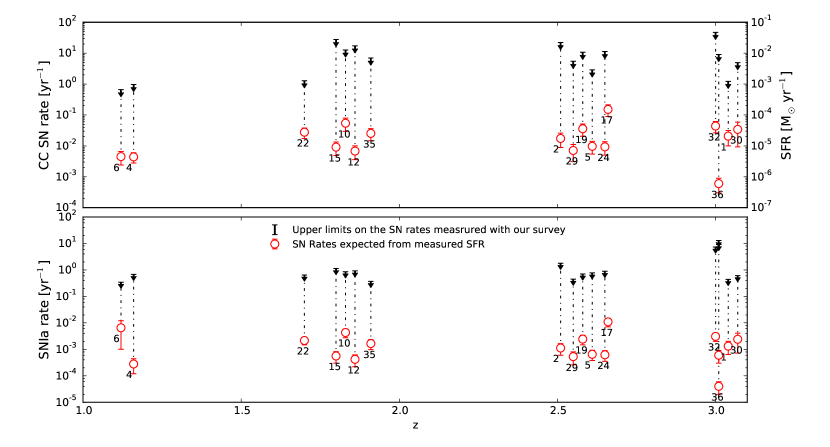
Figure 8: Comparison of the supernova rates limits measured from our survey and those obtained from the SFR published in Riehm et al. (2011). The limits represent 90 % C.L. The numbers label the background galaxies shown in Figure 9. Only the galaxies with multiple images and delay time less than five years (i.e less than the duration of the survey) are considered here.

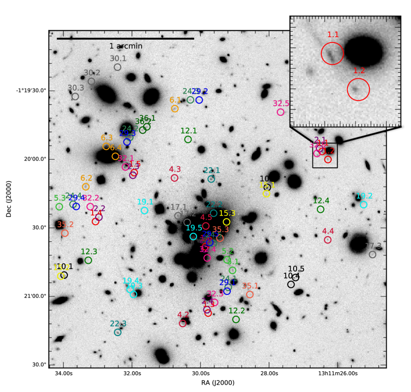
Figure 9: Near-infrared VLT/HAWK-I image overplotted with the 17 background galaxies with 51 multiply images used in Figure 8, Sect. 6 and 8. The predicted magnifications for these galaxies are of order of few magnitudes. As an example, a magnified view of system 1 at $z=3.04$ is shown, in which images 1.1 and 1.2 are magnified by $3.80^{+0.30}_{0.29}$ and $5.58^{+1.21}_{-0.74}$ magnitudes, respectively.

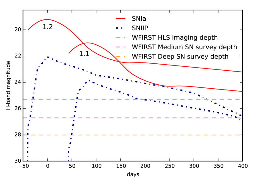
Figure 10: Simulated light curves for SN Ia and IIP in the H band for the multiply-imaged system 1 at $z=3.04$; images 1.1 and 1.2 are magnified $3.80^{+0.30}_{0.29}$ and $5.58^{+1.21}_{-0.74}$ mag, respectively. The time delay between the images is $83^{+77}_{-69}$ days (Riehm et al. 2011). Also shown are the magnitude limits for the three main survey modes planned for WFIRST (Spergel et al. 2013). Without the magnification from A1689, the SN IIP would hardly be observable.

7 A1689 cluster SN rates

In this section, we use the SNe detected in galaxies in A1689 to measure the SN rate in the galaxy cluster. Only $\leq 15\%$ of the galaxies in A1689 show traces of star formation (Laganá et al. 2008), which confirms that most of the members are galaxies with old stellar populations. Hence, it is not surprising, that the SNe we found are SN Ia.

It is not meaningful to discuss the volumetric rate for galaxy clusters, instead the rates are normalized with the cluster total stellar luminosity in one specific band. Here, we used the total B band luminosity and units defined as SNuB$\equiv 10^{-12}\,\rm{SNe}\,L^{-1}_{\odot,B}yr^{-1}$. Furthermore, when SN rates in clusters are compared at different redshifts, it is more useful to normalize by the stellar mass of the galaxy cluster, since the luminosity changes with the stellar population age (Barbary et al. 2012). The units are then SNuM$\equiv 10^{-12}\,\rm{SNe}\,M_{\odot}^{-1}yr^{-1}$.

To determine the SN rate in the galaxy cluster in units SNuB, we used the following relation:

$$R_{Ia}=\frac{N}{T\cdot L_{B}}$$ (10)

where $N$ is the observed number of cluster SNe, $T$ is the total control time and $L_{B}$ is the luminosity of each galaxy member of the cluster in the B band. The total control time represents the amount of time a SN is above the survey detection limit at the cluster redshift. This control time was calculated in an analogous manner as for the volumetric rates. When normalizing by the total stellar mass of the galaxy cluster, the $L_{B}$ is replaced by $M_{*}$ in Eq. 10.

The total stellar luminosity and mass of A1689 within $r_{500}$ (the radius within which the mean cluster density exceeds the critical density by a factor of 500), are adopted from Laganá et al. (2008) $L_{B}=5.99\pm 0.23\cdot 10^{12}L_{\odot,B}$ and $M_{*}=9.0\pm 2.0\cdot 10^{12}M_{\odot}$. They obtained the total luminosity with good precision by combining X-ray and optical data, excluding the background galaxies by using their colours. For the total mass, they used empirical relations between the stellar mass and luminosity of the cluster galaxies.

Table 8: Compilation of SN Ia rates in galaxy clusters

Survey	Number of	Mean	$N_{\rm Ia}$	SN Ia Ratea	Reference
	clusters	redshift		[SNuB$\>h^{2}$]
Clusters in Cappellaro et al. (1999) SN sample	$\cdots$	0.02	12.5	$0.57^{+0.22}_{-0.16}$	Mannucci et al. (2008)
SDSS-II	71	0.084	9	$0.46^{+0.21}_{-0.15}\pm 0.01$	Dilday et al. (2010)
WOOTS	140	0.15	6	$0.73^{+0.45}_{-0.29}\pm 0.04$	Sharon et al. (2007)
A1689	1	0.18	2	$0.14^{+0.19}_{-0.09}\pm 0.01$	This work
SDSS-II	492	0.225	25	$0.68^{+0.17}_{-0.14}\pm 0.02$	Dilday et al. (2010)
HST archival images	6	0.25	1	$0.80^{+1.84}_{-0.65}$	Gal-Yam et al. (2002)
CFHT SNLS	$\cdots$	0.45	3	$0.63^{+1.04}_{-0.33}$	Graham et al. (2008)
HST/ACS survey	15	0.6	6	$0.71^{+0.35}_{-0.24}\pm 0.26$	Sharon et al. (2010)
HST archival images	3	0.9	1	$1.63^{+2.16}_{-1.06}$	Gal-Yam et al. (2002)
HST Cluster SN survey	25	1.14	8	$0.50^{+0.23}_{-0.19}$ ${}^{+0.10}_{-0.09}$	Barbary et al. (2012)

Note: ^a All quoted errors are $1\sigma$ statistical and systematic, where available.

The cluster rate we measure is $0.14^{+0.19}_{-0.09}\pm 0.01$ $\rm SNuB\,$$h^{2}$, where the error bars indicate $1\,\sigma$ confidence intervals, statistical and systematic, respectively. The cluster rate normalized by the stellar mass is $0.10^{+0.13}_{-0.06}\pm 0.02$ in $\rm SNuM\,$$h^{2}$.

Our measurement is based on two SNe Ia detected in one galaxy cluster, and as with most of previous studies, the errors are dominated by small number statistics. In Table 8 we make a comparison of our A1689 SN Ia rate per luminosity in the B band with the existing values from the literature (Mannucci et al. 2008; Dilday et al. 2010; Sharon et al. 2007; Gal-Yam et al. 2002; Graham et al. 2008; Sharon et al. 2010; Barbary et al. 2012)

Thermonuclear SNe have long-lived progenitors, so their rate does directly not reflect the cosmic SFH. Instead, there is an unknown time delay between the formation and explosion of the progenitors. Models are typically parameterized by a delay time distribution (DTD), where a convolution with the SFH gives the SN Ia rate. Cluster galaxies should typically have more uniform stellar populations compared to their counterparts in the field, which in turn, are reflected in a simpler SFH. Barbary et al. (2012) parametrized the SN Ia DTD with a power law $\Psi\propto t^{s}$ and used the approximation of a single burst of star formation at $z=3$. These authors obtained $s=1.41^{+0.47}_{-0.40}$, which is consistent with the DTD estimates in field galaxies. For a detailed discussion, see Barbary et al. (2012) and Maoz et al. (2010).

In Figure 11 we plot our result together with literature values of the SN Ia cluster rates per stellar mass unit (SNuM). We also show the best-fit power-law DTD from Barbary et al. (2012), where $\Psi(t)\propto t^{s}$ with $s=1.41$. Our measured value is consistent with the power law.

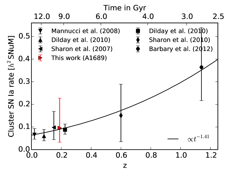
Figure 11: Cluster SN Ia rates in units SNuM $h^{2}$, where SNuM$\equiv 10^{-12}\,\rm{SNe}\,M_{\odot}^{-1}yr^{-1}$. The line shows the best-fit power-law DTD from Barbary et al. (2012), where $\Psi(t)\propto t^{s}$ with $s=1.41$.

8 Expectations for future transient surveys

Here, we discuss the feasibility of finding SNe at $z\gtrsim 2$, where the SN rates are poorly constrained, using current facilities. At these very high redshifts, it is particularly interesting to compare CC rates with those expected from the SFR. These two independent methods can serve as an additional test for the SFH at unprobed redshifts. Moreover, high-$z$ CC SNe can be used for probing the IMF in the early Universe and for studying the possible evolution of the intrinsic properties of CC SNe subtypes.

To assess the necessary depth of a survey, in Figure 12 we plot simulated light curves of SNe Ia, IIn, and IIP in observers frame at redshifts $2.0,2.5,3.0,3.5$, and $4.0$. The yellow band indicates the typical magnifications from a massive galaxy clusters for background objects at those redshifts. Assuming a depth of 24.5 mag in the J band that is suitable for a ground-based survey, it is impossible to observe the light curves at any epoch, without the magnification provided by a cluster lens. For a HST-like survey with a depth of $26.1$ in the F125W and H bands (similar to F160W), SNe IIn and SNe Ia are observable, but the fainter IIP are already too challenging. For this reason, we continue making predictions using the magnification help from the galaxy cluster.

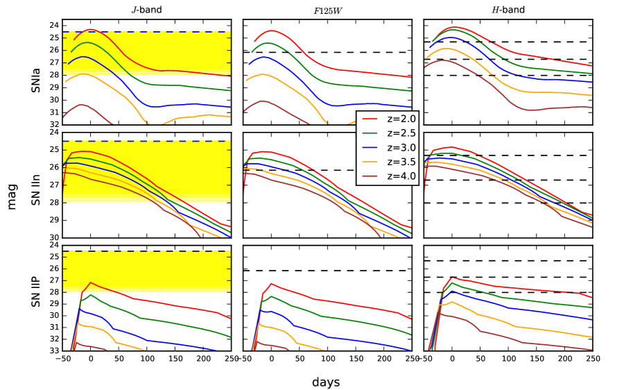
Figure 12: Observer frame light curves for a SN Ia (upper panels), SN IIn (middle panel) and SN IIL (lower panels) in the HAWK-I J, HST F125W and WFIRST H bands, respectively. The horizontal dashed lines indicate the depths assumed in the calculation, 24.5 for the J band and 26.15 for F125W. In the H band the three depths represent the three main survey modes planned for WFIRST (Spergel et al. 2013). The yellow band denotes the average magnification from the galaxy cluster A1689 at the same redshifts in the central region with $2.7\arcmin\times 3.3\arcmin$.

To predict the number of discoverable CC SNe, we used the Mannucci et al. (2007) volumetric SN rate as extrapolated in G09. First, we considered a limiting depth of 24.5 mag in the J band, duration of five years with seven visits per year with a monthly cadence. Second, we considered a limiting depth of 26.15 mag in the F125W band, which is easily obtainable with HST. The results are summarized in Table 9. For the possibility of measuring the CC SN rate, we can assess how many clusters are required to find at least $\sim$$3$ SNe per redshift bin. Even at the redshift bin $\langle z\rangle=2.06$, $\sim$$45$ clusters are required to reach this goal. For the space-based set-up, the number of clusters decreases: at $\langle z\rangle=2.06$, $\sim$$11$ clusters are needed, while at $\langle z\rangle=2.56$, $\sim$$60$. From these estimates, we can conclude that it would be difficult to construct a realistic survey with the existing ground- and space-facilities that would significantly improve the measurement of SN rates at $\langle z\rangle>2.0$, even with the help of a gravitational telescope. This will most likely not be possible before the forthcoming next generation facilities, such as the space-based Wide Field Infrared Survey Telescope (WFIRST), are in operation. The WFIRST will be able to detect SNe to very high-$z$ in the H band (see Figure 12). Without considering the contribution from gravitational lensing, we estimated the expected number of CC SNe to be discovered with WFIRST. During its planned six-years duration, it will dedicate six months spread over two years for a SN search, focusing mainly on SNe Ia to study the possible evolution of the dark energy equation of state parameter (Spergel et al. 2013). However, even a larger number of CC SNe can be expected and the results are shown in Table 10.

Table 9: Expectations for high-$z$ SNe in A1689 FOV

Depth	Filter	Years	Nepochs	Cadence	N${}_{\rm CC}^{a}$	N${}_{\rm CC}^{a}$	N${}_{\rm CC}^{a}$	N${}_{\rm CC}^{a}$
(mag)			/yr	(days)	$1.9\leq z<2.3$	$2.4\leq z<2.8$	$2.9\leq z<3.3$	$3.3\leq z<3.7$
$24.5$	J	$5$	7	30	$0.07\pm 0.01$	$0.010\pm 0.002$	$0.0021\pm 0.0004$	$0.0012\pm 0.0005$
$26.15$	F125W	$5$	7	30	$0.30\pm 0.05$	$0.04\pm 0.01$	$0.011\pm 0.001$	$0.0028\pm 0.0005$

Table 10: Expectations for high-$z$ SNe in WFIRST, H band, for both medium and deep supernova Survey.

N${}_{\rm CC}^{a}$	NCC	NCC	NCC
$1.9\leq z<2.3$	$2.4\leq z<2.8$	$2.9\leq z<3.3$	$3.3\leq z<3.7$
$341\pm 62$	$58\pm 10$	$20\pm 3$	$7.5\pm 1.5$
$1809\pm 327$	$898\pm 160$	$360\pm 63$	$13\pm 2$

Next, we consider the expectations from the multiply-imaged galaxies behind A1689 (presented in Sect. 6) for future surveys. Instead of using the volumetric SN rate, we adopt the SN rate in the resolved galaxies for which we use the predictions derived from the SFR. We simulated three upcoming transient surveys: the Zwicky Transient Facility (ZTF; Bellm 2014), the Large Synoptic Survey Telescope (LSST; LSST Science Collaboration et al. 2009) and WFIRST. The ZTF and LSST are ground-based surveys with 1.2 and 8.4 m telescopes, respectively. The results are shown Table 11. The shallowness makes ZTF not useful for this task. The situation is different for LSST with its improved depth, more suitable filters, and considering the length of the survey. The LSST goal is to revisit the same field $\sim$$164$ and $\sim$$180$ times in the $z$ and $i$ bands, respectively, over ten years, so close epochs can be combined for a better image depth. Around $70$ galaxy clusters with Einstein radii larger than $\theta_{E}>20^{\prime\prime}$ are estimated to be visible to LSST, which would amount to $\sim$$1000$ strongly lensed multiply-imaged galaxies that are detectable with the LSST (LSST Science Collaboration et al. 2009). Thus, extrapolating from our expectation result from A1689 with 17 systems, we may expect roughly $\sim$$40$ strongly lensed SNe Ia with the possibility of measuring the time delay between the multiply images. The WFIRST all-sky survey will also be excellent for this task, since it will offer even more suitable filters for higher-$z$ SNe.

The James Webb Space Telescope (JWST; Gardner et al. 2006) with 6.5 m aperture will have an unmatched resolution and sensitivity reaching up to $\sim$$31$ magnitude from the optical to the mid-IR. With this depth, the aid of gravitational telescopes are not necessarily needed to discover SNe at $z\lesssim 4$. Using the magnification of the galaxy clusters, however, the JWST will be able to discover lensed CC SNe at redshifts exceeding $z=6$ (Pan & Loeb 2013). To achieve this, it will require a dedicated multi-year search towards galaxy clusters with its relatively small field of view of $2.2\arcmin\times 2.2\arcmin$. To improve the lens models of galaxy clusters that will be used as gravitational telescopes by JWST, there is an ongoing 190-orbits HST programme targeting 41 massive clusters named RELICS.

Table 11: Expectations for SNe in the multiply-imaged galaxies in A1689 for future surveys

Survey	Filter	Depth	Years	Nepochs	Cadence	N${}_{\rm CC}^{a}$	N${}_{SN\leavevmode\nobreak\ Ia}^{a}$	$z_{max}^{b}$	$z_{max}^{b}$	N${}_{gal}^{c}$	N${}_{gal}^{c}$
		(mag)		/yr	(days)			CC	SN Ia	CC	SN Ia
ZTF	R	$22.5^{d}$	$3$	7	15	$0.017\pm 0.007$	$0.04\pm 0.03$	1.15	1.15	6	6
ZTF	$i$	$22.5^{d}$	$3$	7	15	$0.03\pm 0.01$	$0.06\pm 0.05$	1.15	1.15	6	6
LSST	$i$	$24.0^{e}$	$10$	7	30	$0.18\pm 0.09$	$0.21\pm 0.17$	3.05	1.70	14	7
LSST	$i$	$25.0^{d}$	$10$	7	30	$0.38\pm 0.18$	$0.26\pm 0.20$	3.05	1.70	23	7
LSST	$z$	$22.76^{e}$	$10$	7	30	$1.14\pm 0.61$	$0.68\pm 0.40$	3.05	3.05	25	33
WFIRST	H	$28.01^{f}$	$2$	3	30	$1.74\pm 0.82$	$0.17\pm 0.08$	3.05	3.05	48	48

9 Summary and conclusions

In this work we present the results of a dedicated ground-based NIR rolling search, accompanied with an optical programme, which is aimed at discovering high-$z$ lensed SNe behind the galaxy cluster Abell 1689. During 2008–2014, we obtained a total of 29 and 19 epochs in the J and $i$ bands, respectively, and discovered five CC SNe behind the cluster and twoSNe Ia associated with A1689. Notably, one of the most distant CC SN ever discovered was found at $z=1.703$ with significant magnification.

Using these discoveries, we compute the volumetric CC SN rates in three redshift bins in the range $0.4<z<1.9$, and put upper limits on the CC SN rates in two additional redshift bins in $1.9<z<2.9$. Upper limits of the volumetric SN Ia rate are also calculated for the same redshift bins. All the measured rates are found to be consistent with previous studies at the corresponding redshifts. We further emphasize the comparably high statistical precision at high redshift, given the modest investment in observing time, which can be obtained using gravitational telescopes.

The impact of systematic uncertainties were calculated for the CC SN rates, which will become increasingly important for upcoming wide-field surveys such as the LSST which are expected to discover a large number of SNe (Lien & Fields 2009). We highlight the need for better understanding CC SN properties, such as the subtype fractions and peak magnitudes, which will affect the systematics budget.

Since the CC SN rate traces the cosmic SFH, we compare our results and literature values to the expected rates calculated from the Madau & Dickinson (2014) SFH. We find that the measured and predicted rates are in good agreement with a scale factor of, $k_{\rm CC}=0.0093\pm 0.0010$ $M_{\odot}^{-1}$.

By simulating ground- and space-based five-year surveys, we explore the possibility of finding lensed SNe at $z\gtrsim 2.0$. We find that there is very little room for improvement with the current facilities and that the next generation of telescopes, for example WFIRST, are needed.

Finally, we estimate the number of strongly lensed SNe with multiple images that can be expected to be discovered behind A1689 by upcoming transient surveys. We find that LSST, and in particular WFIRST, can be expected to find tens of strongly lensed SNe that would allow the time delays between the multiple images to be measured. Until the first light of these surveys, using gravitational telescopes is the only way to find high-$z$ SNe using available ground-based instruments.

Appendix A Supernova detection efficiency

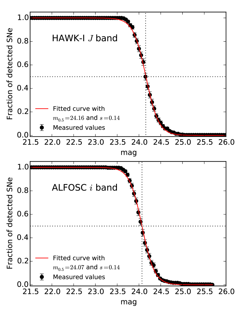
Figure 13: Example of efficiency curves of a detection of point-source transient in the HAWK-I J- and ALFOSC $i$ band data. Error bars represent $1\sigma$ binomial uncertainties. The dotted lines indicate the magnitude at $50\%$ detection efficiency. The magnitudes are given in the Vega system.

We estimated the efficiency of detecting transients in our surveys as a function of magnitude. In order to that we carried out simulations by blindly adding 300 artificial SNe for each of the combined images used in the search. The SNe were modelled with a Moffat PSF fitted to isolated field stars in the images. We used three different approaches to generate the positions of the artificial SNe to study how the detection efficiency is affected by the host brightness: first, we used random positions with low background values; second, close to galaxies; and the third in the coordinates close to the strongly lensed galaxies. The resulting detection efficiency did not change significantly depending on this choice, which is most likely due to the overall bright sky foreground across the image. After that, the simulated data went through the normal image differencing and analysis. For each magnitude bin, we counted the number of successfully detected events. We performed the efficiency simulations for each of the stacked images as used in the HAWK-I (post-survey) and ALFOSC search, and the results are presented in Table 1 and 2, respectively. The efficiency curve as a function of magnitude $m$ can be parameterized with the function

$$\epsilon(m)=\frac{1}{1+e^{(m-m_{0.5})/S}},$$ (11)

where $m_{0.5}$ is the magnitude at $50\%$ detection efficiency and $S$ is the parameter that determines the exponential decline rate. An example of an average efficiency curve for both instruments is shown in Figure 13. The mean value for $s$ is 0.14 for both instruments with a dispersion of 0.01 and 0.03 for HAWK-I and ALFOSC respectively.

The magnitude at $50\%$ detection efficiency correlates with the image depth, which is expected given that the sensitivity of the image determines the magnitude at which detection efficiency drops rapidly as follows:

$$\begin{split}m_{0.5,HAWK\,I-J}=m_{lim}-0.14,\\ m_{0.5,ALFOSC-i}=m_{lim}-0.41.\end{split}$$ (12)

Here, we define image depth as the magnitude of a point source with a $5\sigma$ signal over the background level. In the HAWK-I mosaic images depth varies slightly due to the cross-looking gap between the four chips. HAWK-I has average image depth of $m_{\rm lim}=23.8\pm 0.4$ and $m_{05}=23.7\pm 0.5$, while ALFOSC has $m_{\rm lim}=24.0\pm 0.6$ and $m_{05}=23.4\pm 0.6$.

Appendix B Photometry

Here we present the multi-band photometry from several instruments for the SNe presented in this work. For each observation, we list the modified Julian dates, the filter, and the measured flux with its error. For conversion to magnitude, the zero point is given. We note that the photometry of CAND-821 and CAND-ISAAC are provided in Amanullah et al. (2011a) and G09, respectively.

Table 12: Photometry of the CC SN candidates behind A1689.

MJD	Filter	Flux	Flux	Zero point
(days)			error	(mag)
CAND-1392
$55387.9$	$i$	$-320$	840	32.51
$55564.17$	$i$	$3300$	400	$\cdots$
$55599.12$	$i$	$630$	310	$\cdots$
$55604.11$	$i$	$1400$	1000	$\cdots$
$55650.11$	$i$	$-550$	380	$\cdots$
$55387.98$	$g$	$-690$	1040	32.70
$55564.22$	$g$	$600$	200	$\cdots$
$55599.19$	$g$	$370$	210	$\cdots$
$55650.03$	$g$	$-10$	230	$\cdots$
$55387.95$	$r$	$-270$	630	32.20
$55564.24$	$r$	$1200$	200	$\cdots$
$55599.17$	$r$	$-20$	150	$\cdots$
$55604.16$	$r$	$-200$	300	$\cdots$
$55650.08$	$r$	$140$	290	$\cdots$
CAND-669
$54943.0$	$i$	$1300$	1300	$32.86$
$54987.9$	$i$	$240$	600	$\cdots$
$55006.92$	$i$	$330$	490	$\cdots$
$54862.26$	$J$	$30$	90	$30.67$
$54892.23$	$J$	$1540$	90	$\cdots$
$54914.32$	$J$	$1160$	100	$\cdots$
$54916.19$	$J$	$1210$	80	$\cdots$
$54949.1$	$J$	$670$	80	$\cdots$
$54990.11$	$J$	$380$	130	$\cdots$
$55016.05$	$J$	$220$	160	$\cdots$
$55018.1$	$J$	$360$	150	$\cdots$
$55019.97$	$J$	$240$	250	$\cdots$
$54919.16$	$NB1060$	$250$	110	$30.37$
$54923.3$	$NB1060$	$250$	100	$\cdots$
$54948.99$	$NB1060$	$170$	150	$\cdots$
$54966.0$	$NB1060$	$160$	110	$\cdots$
$54968.99$	$NB1060$	$0$	160	$\cdots$
$54979.07$	$NB1060$	$60$	120	$\cdots$
$55008.98$	$NB1060$	$0$	210	$\cdots$
$55009.96$	$NB1060$	$-110$	110	$\cdots$
$55028.0$	$NB1060$	$40$	110	$\cdots$
$55035.01$	$NB1060$	$140$	260	$\cdots$
$55054.97$	$NB1060$	$220$	150	$\cdots$
$55056.0$	$NB1060$	$320$	140	$\cdots$
CAND-10658
$56366.26$	$J$	$30$	30	$29.87$
$56415.91$	$J$	$-30$	30	$\cdots$
$56450.79$	$J$	$-10$	40	$\cdots$
$56728.78$	$J$	$1070$	40	$\cdots$
$56796.06$	$J$	$1450$	50	$\cdots$
$56828.10$	$J$	$570$	160	$\cdots$
$56858.99$	$J$	$370$	40	$\cdots$
CAND-10662
$56366.26$	$J$	$20$	20	$29.60$
$56383.26$	$J$	$0$	20	$\cdots$
$56415.91$	$J$	$-10$	20	$\cdots$
$56450.79$	$J$	$50$	30	$\cdots$
$56728.78$	$J$	$230$	30	$\cdots$
$56796.06$	$J$	$280$	40	$\cdots$
$56828.1$	$J$	$170$	120	$\cdots$
$56858.99$	$J$	$170$	40	$\cdots$

Table 13: Photometry of the SN Ia candidates.

MJD	Filter	Flux	Flux	Zero point
(days)			error	(mag)
CAND-1208
$55273.14$	$i$	-1500	1500	$32.50$
$55333.98$	$i$	$108800$	500	$\cdots$
$55337.0$	$i$	$92600$	2100	$\cdots$
$55359.97$	$i$	$49000$	1000	$\cdots$
$55387.9$	$i$	$19100$	1200	$\cdots$
$55564.17$	$i$	$-350$	430	$\cdots$
$55337.96$	$g$	$46800$	400	$32.67$
$55359.92$	$g$	$8200$	200	$\cdots$
$55387.98$	$g$	$4500$	1200	$\cdots$
$55273.09$	$r$	$-620$	370	$32.22$
$55333.94$	$r$	$76400$	400	$\cdots$
$55336.95$	$r$	$62800$	400	$\cdots$
$55359.94$	$r$	$22000$	500	$\cdots$
$55387.95$	$r$	$10000$	1000	$\cdots$
$55564.24$	$r$	$-210$	430	$\cdots$
$55382.41$	$F814W$	$1420$	30	$30.0$
$55382.82$	$F814W$	$1410$	30	$\cdots$
$55383.40$	$F814W$	$1380$	30	$\cdots$
$55384.59$	$F814W$	$1370$	30	$\cdots$
$55372.16$	$F814W$	$1990$	40	$\cdots$
$55385.73$	$F814W$	$1310$	30	$\cdots$
CAND-802
$54949.16$	$J$	$10$	30	$29.58$
$54990.13$	$J$	$680$	50	$\cdots$
$55018.06$	$J$	$620$	40	$\cdots$
$56366.26$	$J$	$-20$	30	$\cdots$
$54943.0$	$i$	$260$	780	$31.96$
$54987.9$	$i$	$1700$	300	$\cdots$
$55006.92$	$i$	$2100$	200	$\cdots$
$55054.97$	$NB1060$	$640$	80	$30.41$
CAND-7169
$56366.26$	$J$	$100$	140	$29.60$
$56381.26$	$J$	$230$	140	$\cdots$
$56383.27$	$J$	$180$	150	$\cdots$
$56385.26$	$J$	$190$	140	$\cdots$
$56408.29$	$J$	$2600$	300	$\cdots$
$56419.21$	$J$	$1700$	200	$\cdots$
$56420.24$	$J$	$1700$	200	$\cdots$
$56448.14$	$J$	$1200$	130	$\cdots$
$56449.17$	$J$	$1190$	120	$\cdots$

References

- Alard (2000) Alard, C. 2000, A&AS, 144, 363
- Alard & Lupton (1998) Alard, C. & Lupton, R. H. 1998, ApJ, 503, 325
- Alavi et al. (2014) Alavi, A., Siana, B., Richard, J., et al. 2014, ApJ, 780, 143
- Amanullah et al. (2011a) Amanullah, R., Goobar, A., Clément, B., et al. 2011a, ApJ, 742, L7
- Amanullah et al. (2011b) Amanullah, R., Goobar, A., Johansson, J., et al. 2011b, Central Bureau Electronic Telegrams, 2642, 1
- Amanullah et al. (2008) Amanullah, R., Stanishev, V., Goobar, A., et al. 2008, A&A, 486, 375
- Anderson et al. (2014) Anderson, J. P., González-Gaitán, S., Hamuy, M., et al. 2014, ApJ, 786, 67
- Astier et al. (2006) Astier, P., Guy, J., Regnault, N., et al. 2006, A&A, 447, 31
- Barbary et al. (2012) Barbary, K., Aldering, G., Amanullah, R., et al. 2012, ApJ, 745, 32
- Bazin et al. (2009) Bazin, G., Palanque-Delabrouille, N., Rich, J., et al. 2009, A&A, 499, 653
- Bell et al. (2003) Bell, E. F., McIntosh, D. H., Katz, N., & Weinberg, M. D. 2003, ApJS, 149, 289
- Bellm (2014) Bellm, E. 2014, in The Third Hot-wiring the Transient Universe Workshop, ed. P. R. Wozniak, M. J. Graham, A. A. Mahabal, & R. Seaman, 27–33
- Bertin (2006) Bertin, E. 2006, in Astronomical Society of the Pacific Conference Series, Vol. 351, Astronomical Data Analysis Software and Systems XV, ed. C. Gabriel, C. Arviset, D. Ponz, & S. Enrique, 112
- Bertin & Arnouts (1996) Bertin, E. & Arnouts, S. 1996, A&AS, 117, 393
- Bertin et al. (2002) Bertin, E., Mellier, Y., Radovich, M., et al. 2002, in Astronomical Society of the Pacific Conference Series, Vol. 281, Astronomical Data Analysis Software and Systems XI, ed. D. A. Bohlender, D. Durand, & T. H. Handley, 228
- Blondin & Tonry (2007) Blondin, S. & Tonry, J. L. 2007, ApJ, 666, 1024
- Bolton & Burles (2003) Bolton, A. S. & Burles, S. 2003, ApJ, 592, 17
- Bolzonella et al. (2000) Bolzonella, M., Miralles, J.-M., & Pelló, R. 2000, A&A, 363, 476
- Botticella et al. (2008) Botticella, M. T., Riello, M., Cappellaro, E., et al. 2008, A&A, 479, 49
- Botticella et al. (2012) Botticella, M. T., Smartt, S. J., Kennicutt, R. C., et al. 2012, A&A, 537, A132
- Broadhurst et al. (2005) Broadhurst, T., Benítez, N., Coe, D., et al. 2005, ApJ, 621, 53
- Burns et al. (2011) Burns, C. R., Stritzinger, M., Phillips, M. M., et al. 2011, AJ, 141, 19
- Calzetti et al. (2000) Calzetti, D., Armus, L., Bohlin, R. C., et al. 2000, ApJ, 533, 682
- Cappellaro et al. (2015) Cappellaro, E., Botticella, M. T., Pignata, G., et al. 2015, A&A, 584, A62
- Cappellaro et al. (1999) Cappellaro, E., Evans, R., & Turatto, M. 1999, A&A, 351, 459
- Cardelli et al. (1989) Cardelli, J. A., Clayton, G. C., & Mathis, J. S. 1989, ApJ, 345, 245
- Casali et al. (2006) Casali, M., Pirard, J.-F., Kissler-Patig, M., et al. 2006, in Society of Photo-Optical Instrumentation Engineers (SPIE) Conference Series, Vol. 6269, Society of Photo-Optical Instrumentation Engineers (SPIE) Conference Series, 0
- Chatzopoulos et al. (2011) Chatzopoulos, E., Wheeler, J. C., Vinko, J., et al. 2011, ApJ, 729, 143
- Coe et al. (2010) Coe, D., Benítez, N., Broadhurst, T., & Moustakas, L. A. 2010, ApJ, 723, 1678
- Czoske (2004) Czoske, O. 2004, in IAU Colloq. 195: Outskirts of Galaxy Clusters: Intense Life in the Suburbs, ed. A. Diaferio, 183–187
- Dahlen et al. (2008) Dahlen, T., Strolger, L.-G., & Riess, A. G. 2008, ApJ, 681, 462
- Dahlen et al. (2012) Dahlen, T., Strolger, L.-G., Riess, A. G., et al. 2012, ApJ, 757, 70
- Dahlen et al. (2004) Dahlen, T., Strolger, L.-G., Riess, A. G., et al. 2004, ApJ, 613, 189
- Di Carlo et al. (2002) Di Carlo, E., Massi, F., Valentini, G., et al. 2002, ApJ, 573, 144
- Diego et al. (2015) Diego, J. M., Broadhurst, T., Benitez, N., et al. 2015, MNRAS, 446, 683
- Dilday et al. (2010) Dilday, B., Smith, M., Bassett, B., et al. 2010, ApJ, 713, 1026
- Fabbro (2001) Fabbro, S. 2001, PhD thesis, Université Denis Diderot, Paris, France
- Fassia et al. (2000) Fassia, A., Meikle, W. P. S., Vacca, W. D., et al. 2000, MNRAS, 318, 1093
- Frye et al. (2012) Frye, B. L., Hurley, M., Bowen, D. V., et al. 2012, ApJ, 754, 17
- Gal-Yam et al. (2002) Gal-Yam, A., Maoz, D., & Sharon, K. 2002, MNRAS, 332, 37
- Gardner et al. (2006) Gardner, J. P., Mather, J. C., Clampin, M., et al. 2006, Space Sci. Rev., 123, 485
- Goobar & Leibundgut (2011) Goobar, A. & Leibundgut, B. 2011, Annual Review of Nuclear and Particle Science, 61, 251
- Goobar et al. (2009) Goobar, A., Paech, K., Stanishev, V., et al. 2009, A&A, 507, 71
- Graham et al. (2008) Graham, M. L., Pritchet, C. J., Sullivan, M., et al. 2008, AJ, 135, 1343
- Graur et al. (2015) Graur, O., Bianco, F. B., & Modjaz, M. 2015, MNRAS, 450, 905
- Graur et al. (2011) Graur, O., Poznanski, D., Maoz, D., et al. 2011, MNRAS, 417, 916
- Grillo et al. (2015) Grillo, C., Karman, W., Suyu, S. H., et al. 2016, ApJ, 822, 78
- Gunnarsson & Goobar (2003) Gunnarsson, C. & Goobar, A. 2003, A&A, 405, 859
- Harrison & Noonan (1979) Harrison, E. R. & Noonan, T. W. 1979, ApJ, 232, 18
- Hatano et al. (1998) Hatano, K., Branch, D., & Deaton, J. 1998, ApJ, 502, 177
- Holz (2001) Holz, D. E. 2001, ApJ, 556, L71
- Horiuchi et al. (2011) Horiuchi, S., Beacom, J. F., Kochanek, C. S., et al. 2011, ApJ, 738, 154
- Hsiao et al. (2007) Hsiao, E. Y., Conley, A., Howell, D. A., et al. 2007, ApJ, 663, 1187
- Jullo et al. (2007) Jullo, E., Kneib, J.-P., Limousin, M., et al. 2007, New Journal of Physics, 9, 447
- Kelly et al. (2015) Kelly, P. L., Rodney, S. A., Treu, T., et al. 2015, Science, 347, 1123
- Kelly et al. (2016) Kelly, P. L., Rodney, S. A., Treu, T., et al., 2016, ApJ, 819, L8
- Kolatt & Bartelmann (1998) Kolatt, T. S. & Bartelmann, M. 1998, MNRAS, 296, 763
- Kovner & Paczynski (1988) Kovner, I. & Paczynski, B. 1988, ApJ, 335, L9
- Laganá et al. (2008) Laganá, T. F., Lima Neto, G. B., Andrade-Santos, F., & Cypriano, E. S. 2008, A&A, 485, 633
- Lemze et al. (2009) Lemze, D., Broadhurst, T., Rephaeli, Y., Barkana, R., & Umetsu, K. 2009, ApJ, 701, 1336
- Li et al. (2011) Li, W., Leaman, J., Chornock, R., et al. 2011, MNRAS, 412, 1441
- Lien & Fields (2009) Lien, A. & Fields, B. D. 2009, J. Cosmology Astropart. Phys., 1, 047
- Limousin et al. (2007) Limousin, M., Richard, J., Jullo, E., et al. 2007, ApJ, 668, 643
- LSST Science Collaboration et al. (2009) LSST Science Collaboration, Abell, P. A., Allison, J., et al. 2009, ArXiv e-prints, [arXiv: 0912.0201]
- Madau & Dickinson (2014) Madau, P. & Dickinson, M. 2014, ARA&A, 52, 415
- Mannucci et al. (2007) Mannucci, F., Della Valle, M., & Panagia, N. 2007, MNRAS, 377, 1229
- Mannucci et al. (2008) Mannucci, F., Maoz, D., Sharon, K., et al. 2008, MNRAS, 383, 1121
- Maoz et al. (2010) Maoz, D., Sharon, K., & Gal-Yam, A. 2010, ApJ, 722, 1879
- Martini et al. (2007) Martini, P., Mulchaey, J. S., & Kelson, D. D. 2007, ApJ, 664, 761
- Mattila et al. (2012) Mattila, S., Dahlen, T., Efstathiou, A., et al. 2012, ApJ, 756, 111
- Melinder et al. (2012) Melinder, J., Dahlen, T., Mencía Trinchant, L., et al. 2012, A&A, 545, A96
- Narasimha & Chitre (1988) Narasimha, D. & Chitre, S. M. 1988, ApJ, 332, 75
- Neill et al. (2006) Neill, J. D., Sullivan, M., Balam, D., et al. 2006, AJ, 132, 1126
- Nobili et al. (2005) Nobili, S., Amanullah, R., Garavini, G., et al. 2005, A&A, 437, 789
- Nordin et al. (2014) Nordin, J., Rubin, D., Richard, J., et al. 2014, MNRAS, 440, 2742
- Oguri (2007) Oguri, M. 2007, ApJ, 660, 1
- Oguri & Kawano (2003) Oguri, M. & Kawano, Y. 2003, MNRAS, 338, L25
- Pan & Loeb (2013) Pan, T. & Loeb, A. 2013, MNRAS, 435, L33
- Patel et al. (2014) Patel, B., McCully, C., Jha, S. W., et al. 2014, ApJ, 786, 9
- Pirard et al. (2004) Pirard, J.-F., Kissler-Patig, M., Moorwood, A., et al. 2004, in Society of Photo-Optical Instrumentation Engineers (SPIE) Conference Series, Vol. 5492, Ground-based Instrumentation for Astronomy, ed. A. F. M. Moorwood & M. Iye, 1763–1772
- Porciani & Madau (2000) Porciani, C. & Madau, P. 2000, ApJ, 532, 679
- Postman et al. (2012) Postman, M., Coe, D., Benítez, N., et al. 2012, ApJS, 199, 25
- Refsdal (1964) Refsdal, S. 1964, MNRAS, 128, 307
- Richardson et al. (2002) Richardson, D., Branch, D., Casebeer, D., et al. 2002, AJ, 123, 745
- Richardson et al. (2014) Richardson, D., Jenkins, III, R. L., Wright, J., & Maddox, L. 2014, AJ, 147, 118
- Riehm et al. (2011) Riehm, T., Mörtsell, E., Goobar, A., et al. 2011, A&A, 536, A94
- Riello & Patat (2005) Riello, M. & Patat, F. 2005, MNRAS, 362, 671
- Rodney et al. (2015a) Rodney, S. A., Patel, B., Scolnic, D., et al. 2015a, ApJ, 811, 70
- Rodney et al. (2015b) Rodney, S. A., Patel, B., Scolnic, D., et al. 2015b, ApJ, 811, 70
- Rodney et al. (2014) Rodney, S. A., Riess, A. G., Strolger, L.-G., et al. 2014, AJ, 148, 13
- Salpeter (1955) Salpeter, E. E. 1955, ApJ, 121, 161
- Scalzo et al. (2010) Scalzo, R. A., Aldering, G., Antilogus, P., et al. 2010, ApJ, 713, 1073
- Scannapieco & Bildsten (2005) Scannapieco, E. & Bildsten, L. 2005, ApJ, 629, L85
- Sharon et al. (2010) Sharon, K., Gal-Yam, A., Maoz, D., et al. 2010, ApJ, 718, 876
- Sharon et al. (2007) Sharon, K., Gal-Yam, A., Maoz, D., Filippenko, A. V., & Guhathakurta, P. 2007, ApJ, 660, 1165
- Smith et al. (2009) Smith, N., Silverman, J. M., Chornock, R., et al. 2009, ApJ, 695, 1334
- Spergel et al. (2013) Spergel, D., Gehrels, N., Breckinridge, J., et al. 2013, ArXiv e-prints
- Stanishev et al. (2009) Stanishev, V., Goobar, A., Paech, K., et al. 2009, A&A, 507, 61
- Strolger et al. (2015) Strolger, L.-G., Dahlen, T., Rodney, S. A., et al. 2015, ApJ, 813, 93
- Sullivan et al. (2000) Sullivan, M., Ellis, R., Nugent, P., Smail, I., & Madau, P. 2000, MNRAS, 319, 549
- Taddia et al. (2013) Taddia, F., Stritzinger, M. D., Sollerman, J., et al. 2013, A&A, 555, A10
- Taylor et al. (2014) Taylor, M., Cinabro, D., Dilday, B., et al. 2014, ApJ, 792, 135
- Trenti & Stiavelli (2008) Trenti, M. & Stiavelli, M. 2008, ApJ, 676, 767
- Treu et al. (2015) Treu, T., Schmidt, K. B., Brammer, G. B., et al. 2015, ApJ, 812, 114
- Umetsu et al. (2015) Umetsu, K., Sereno, M., Medezinski, E., et al. 2015, ApJ, 806, 207
- Zitrin et al. (2014) Zitrin, A., Redlich, M., & Broadhurst, T. 2014, ApJ, 789, 51
- Zwicky (1937) Zwicky, F. 1937, ApJ, 86, 217
- Zwicky (1938) Zwicky, F. 1938, ApJ, 88, 529