Lévy Transport in Slab Geometry of Inhomogeneous Media

Abstract

We present a physical example, where a fractional (both in space and time) Schrödinger equation appears only as a formal effective description of diffusive wave transport in complex inhomogeneous media. This description is a result of the parabolic equation approximation that corresponds to the paraxial small angle approximation of the fractional Helmholtz equation. The obtained effective quantum dynamics is fractional in both space and time. As an example, Lévy flights in an infinite potential well are considered numerically. An analytical expression for the effective wave function of the quantum dynamics is obtained as well.

I Introduction

Application of the fractional calculus to quantum processes is a new and fast developing part of quantum physics, which studies nonlocal quantum phenomena kusnezov ; laskin1 ; west ; WBG . It aims to explore nonlocal effects found for either long-range interactions or time-dependent processes with many scales WBG ; bouchaud ; klafter . As it is shown in the seminal papers laskin1 ; west , the fractional concept can be introduced in quantum physics by means of the Feynman propagator for non-relativistic quantum mechanics in complete analogy with the Brownian path integrals feynman . The path integral approach for Lévy stable processes, leading to the fractional diffusion equation, can be extended to a quantum Feynman-Lévy measure, which leads to natural appearance of the space fractional Schrödinger equation laskin1 ; west .

A way of introduction of a fractional time derivative in quantum mechanics is not so “easy”. It is tempting to introduce it in the quantum mechanics by analogy with the fractional Fokker-Planck equation (FFPE) by means of the Wick rotation of time $t\rightarrow-it/\hbar$ naber . However this way is completely vague from its physical interpretation. First, it violates Stone’s theorem on the one-parameter unitary group stone . Another important discrepancy between the Fokker-Planck and the Schrödinger equations is that the latter is the fundamental quantum-mechanical postulate, while the former is just an asymptotic limit of a kinetic equation for the Markovian random process. It is worth noting that, contrary to the space fractional derivative, the fractional time Schrödinger equation (FSE) describes non-Markovian evolution with a memory effect. For the Markovian processes the link between the Schrödinger equation and the Fokker-Planck equation is established by the path integral presentation kac ; schulman ; chaichian . Contrary to this for the non-Markovian processes this path integral relation is broken due to violation of the Stone theorem, therefore the relation between FSE and FFPE is broken as well.

However, these arguments do not discard a mathematical attractivity of the FSE. As shown in iom2009 ; iom2011 , the FSE is an effective way to describe the dynamics of a quantum system interacting with the environment. In this case, fractional time derivative is an effect of the interaction of the quantum system with the environment, where part of the quantum information is lost iom2011 ; wo2010 . Therefore, in the paper we consider a physical example of a fractional (both in space and time) Schrödinger equation, which appears only as a formal effective description of diffusive wave transport in complex inhomogeneous media. We show that considering FFPE in the parabolic equation approximation, which corresponds to the paraxial small angle approximation, one can obtain the FSE as an effective way to solve fractional eigenvalue problem in slab geometry, where the paraxial small angle approximation is naturally applied. The method of parabolic equation approximation was first applied by Leontovich in study of radio-waves spreading leontovich and later developed in detail by Khokhlov khohlov (see also tappert ). In modern experimental and theoretical research, it naturally appears in investigations of a wave propagation in random optical lattices moti1 ; moti2 ; moti3 ; moti4 .

The FFPE is one of the most general asymptotic description of a wave-diffusion transport in inhomogeneous media WGMN ; mainardi1 . For example, fractional calculus description has been introduced to describe the wave propagation at anomalous diffusive oscillations in the Lorentz (Cauchy) pair plasma with dust impurities turski1 , random walk of optic rays in Lévy lens LevyLens , fractional wave-diffusion in heterogeneous media mainardi ; Meerschaert as well as seismic waves mainardi2 ; Casasanta .

This paper is organized as follows. In Section 2 we give a brief introduction to fractional calculus and Mittag-Leffler functions. FFPE in a slab geometry is considered in Section 3. By using paraxial approximation we derive the corresponding FSE as the parabolic equation approximation for the considered process. In Section 4, the obtained model is considered as a kind of a generalisation of the fractional quantum mechanics. Summary is given in Section 5.

II Mathematical tools: Fractional calculus briefly

Fractional derivation was developed as a generalization of integer order derivatives and is defined as the inverse operation to the fractional integral. Fractional integration of the order of $\alpha$ is defined by the operator (see e.g. WBG ; klafter ; podlubny ; oldham ; SKM )

$${}_{a}I_{x}^{\alpha}f(x)=\frac{1}{\Gamma(\alpha)}\int_{a}^{x}f(y)(x-y)^{\alpha-1}dy\,,$$

where $\alpha>0,~{}x>a$ and $\Gamma(z)$ is the Gamma function. Therefore, the fractional derivative is defined as the inverse operator to ${}_{a}I_{x}^{\alpha}$, namely ${}_{a}D_{x}^{\alpha}f(x)={}_{a}I_{x}^{-\alpha}f(x)$ and ${}_{a}I_{x}^{\alpha}={}_{a}D_{x}^{-\alpha}$. Its explicit form is

$${}_{a}D_{x}^{\alpha}f(x)=\frac{1}{\Gamma(-\alpha)}\int_{a}^{x}f(y)(x-y)^{-1-\alpha}dy\,.$$

For arbitrary $\alpha>0$ this integral diverges, and as a result of this a regularization procedure is introduced with two alternative definitions of ${}_{a}D_{x}^{\alpha}$. For an integer $n$ defined as $n-1<\alpha<n$, one obtains the Riemann-Liouville fractional derivative of the form

$${}_{a}^{RL}D_{x}^{\alpha}f(x)=\frac{d^{n}}{dx^{n}}{}_{a}I_{x}^{n-\alpha}f(x)\,,$$ (1)

and fractional derivative in the Caputo form mainardi

$${}_{a}^{C}D_{x}^{\alpha}f(x)={}_{a}I_{x}^{n-\alpha}f^{(n)}(x)\,,~{}~{}~{}f^{(n)}(x)\equiv\frac{d^{n}}{dx^{n}}f(x)\,.$$ (2)

There is no constraint on the lower limit $a$. For example, when $a=0$, one has ${}_{0}^{RL}D_{x}^{\alpha}x^{\beta}=\frac{x^{\beta-\alpha}\Gamma(\beta+1)}{\Gamma(\beta+1-\alpha)}$ and

$${}_{0}^{C}D_{x}^{\alpha}f(x)={}_{0}^{RL}D_{x}^{\alpha}f(x)-\sum_{k=0}^{n-1}f^{(k)}(0^{+})\frac{x^{k-\alpha}}{\Gamma(k-\alpha+1)}\,,$$

and ${}_{a}^{C}D_{x}^{\alpha}[1]=0$, while ${}_{0}^{RL}D_{x}^{\alpha}[1]=x^{-\alpha}/\Gamma(1-\alpha)$. When $a=-\infty$, the resulting Weyl derivative is

$${}_{-\infty}\mathcal{W}_{x}^{\alpha}\equiv{}_{-\infty}^{W}D_{x}^{\alpha}={}_{-\infty}^{RL}D_{x}^{\alpha}={}_{-\infty}^{C}D_{x}^{\alpha}\,.$$ (3)

One also has ${}_{-\infty}^{W}D_{x}^{\alpha}e^{x}=e^{x}$ This property is convenient for the Fourier transform

$$\mathcal{F}\left[{}_{-\infty}\mathcal{W}_{x}^{\alpha}f(x)\right]=(ik)^{\alpha}\bar{f}(k)\,,$$ (4)

where $\mathcal{F}[f(x)]=\bar{f}(k)$. This fractional derivation with the fixed lower limit is also called the left fractional derivative. One can introduce the right fractional derivative, where the upper limit $a$ is fixed and $a>x$. For example, the right Weyl derivative is

$${}_{x}\mathcal{W}_{\infty}^{\alpha}f(z)=\frac{1}{\Gamma(-\alpha)}\int_{x}^{\infty}\frac{f(y)dy}{(y-x)^{1+\alpha}}\,.$$ (5)

The Laplace transform of the Caputo fractional derivative yields

$$\mathcal{L}[{}_{0}^{C}D_{x}^{\alpha}f(x)]=s^{\alpha}\tilde{f}(s)-\sum_{k=0}^{n-1}f^{(k)}(0^{+})s^{\alpha-1-k}\,,$$ (6)

where $\mathcal{L}[f(x)]=\tilde{f}(s)$, that is convenient for the present analysis, where the initial conditions are supposed in terms of integer derivatives. We also use here a convolution rule for $0<\alpha<1$

$$\mathcal{L}[{}_{0}I_{x}^{\alpha}f(x)]=s^{-\alpha}\tilde{f}(s)\,.$$ (7)

The fractional derivative from an exponential function can be simply calculated as well by virtue of the Mittag–Leffler function (see e.g., podlubny ; bateman ):

$$E_{\gamma,\delta}(z)=\sum_{k=0}^{\infty}\frac{z^{k}}{\Gamma(\gamma k+\delta)}\,,$$ (8)

where $\gamma,\delta>0$ and for $\delta=1$ one also obtains the Mittag–Leffler function in one parameter $E_{\gamma,1}(z)=E_{\gamma}(z)$ podlubny . Therefore, we have the following expression

$${}_{0}^{RL}D_{x}^{\alpha}e^{\lambda x}=x^{-\alpha}E_{1,1-\alpha}(\lambda x)\,.$$ (9)

while for the Caputo fractional derivative the Mittag-Leffler function $E_{\gamma}(z^{\gamma})$ is the eigenfunction

$${}_{0}^{C}D_{z}^{\gamma}E_{\gamma}(\lambda z^{\gamma})=\lambda E_{\gamma}(\lambda z^{\gamma})\,.$$ (10)

The Laplace transform of the Mittag-Leffler function (8) is given by podlubny

$$\mathcal{L}\left[z^{\delta-1}E_{\gamma,\delta}(\pm\omega z^{\gamma})\right](s)=\frac{s^{\gamma-\delta}}{s^{\gamma}\mp\omega},\quad\Re(s)>|\omega|^{1/\gamma}.$$ (11)

For the Mittag-Leffler function (8) the following formula holds bateman

$$E_{\gamma,\delta}(-z)=-\sum_{n=1}^{\infty}\frac{(-z)^{-n}}{\Gamma(\delta-\beta n)},\quad|z|>1,$$ (12)

from where it follows the following asymptotic behavior

$$E_{\gamma,\delta}(-z)=\frac{z^{-1}}{\Gamma(\delta-\beta)},\quad|z|\rightarrow\infty.$$ (13)

III FFPE in slab geometry: parabolic equation approximation

We begin our analysis by considering a general form of the FFPE for the 2D slab geometry described by dimensionless $(r,z)$ variables, where $z\in(0,\,\infty)$ and $r\in[-L,\,L]$. Therefore the probability distribution function $P(r,z,t)$ to find a particle at the point $(r,z)$ at time $t$ is governed by the FFPE, which consists of both the Caputo and the Riemann-Liouville fractional derivatives. In what follows, the low limit of the Caputo derivatives is $a=0$, therefore, we use the following notation

$$\partial_{x}^{\alpha}\equiv{}_{0}^{C}D_{x}^{\alpha}\,,~{}~{}~{}x=z,\,t\,.$$ (1)

These fractional derivatives are used for the dimensionless time $t\in(0,\,\infty)$ and the longitudinal direction $z(0,\,\infty)$. In this case the Laplace transform (6) is determined explicitly by the initial condition $P(r,z,t=0)=P_{0}(r,z)$ and its evolution in time at $z=0$. For the orthogonal direction $r\in[-L,\,L]$, the following notation is used

$$\mathcal{D}_{|x|}^{\alpha}\equiv{}_{-L}^{RL}D_{x}^{\alpha}+{}_{x}^{RL}D_{L}^{\alpha}\,,~{}~{}x=r\,.$$ (2)

The FFPE reads

$$\partial_{t}^{\alpha}P=\mathcal{K}_{\beta}\partial_{z}^{\beta}P+\mathcal{K}_{\beta}\mathcal{D}_{|r|}^{\beta}P\,,$$ (3)

where $\mathcal{K}_{\beta}$ is a diffusivity of the media, while $0<\alpha<1$ and $1<\beta<2$.

The FFPE (3) is a general form of space-time fractional equations. It describes both waves and relaxation processes in a variety of applications like diffusion-wave phenomena in inhomogeneous media mainardi1 ; turski1 ; LevyLens ; mainardi ; Meerschaert ; mainardi2 . It should be stressed that fractional space derivatives describe Lévy flights klafter . In particular, we specify here optical ray dynamics in Lévy glasses LevyLens , where Lévy flights can be described by Eq. (3). Another interesting phenomenon, which is described by Eq. (3), is superdiffusion of ultra-cold atoms in an optical lattice nirD

Therefore, our main concern is now the Helmholtz fractional equation, which relates to the Lévy process. The next step of the analysis is the separation of variables (see e.g. klafter ) according the following separation ansatz

$$P(r,z,t)=\int_{-i\infty+\sigma}^{+i\infty+\sigma}E_{\alpha}(\omega t^{\alpha})W(r,z,\omega)d\omega\,,$$ (4)

where $E_{\alpha}(\omega t^{\alpha})$ is the Mittag-Leffler function (8), while $W(r,z,\omega)$ is determined from the fractional Helmholtz equation

$$\partial_{z}^{\beta}W+\mathcal{D}_{|r|}^{\beta}W+\omega_{\beta}W=0\,,$$ (5)

where $\omega_{\beta}=\frac{\omega}{\mathcal{K}_{\beta}}$. When the height $L$ is less than the Lévy flight lengths in the longitudinal direction, the transport is of a small grazing angle with respect to the longitudinal direction. We are looking for the solution $W(z,r,\omega)$ in the form

$$W(z,r.\omega)=e^{ikz}u(z,r,\omega),$$ (6)

which after substitution in Eq. (5) yields the following integration

$$\partial_{z}^{\beta}W(z,r,\omega)=\frac{1}{\Gamma(2-\beta)}\int_{0}^{z}(z-z^{\prime})^{2-\beta-1}\frac{d^{2}}{dz^{\prime 2}}\left[e^{ikz^{\prime}}u(z^{\prime},r,\omega)\right]dz\,.$$ (7)

Note that the “initial” conditions at $z=0$ for both $u$ and $W$ are the same: $u(z=0)=W(z=0)$.

Now the parabolic equation in the paraxial approximation can be obtained. Taking into account that $u(z,r,\omega)$ is a slowly-varying function of $z$, such that

$$\Big{|}\frac{\partial^{2}u}{\partial z^{2}}\Big{|}\ll\Big{|}2k\frac{\partial u}{\partial z}\Big{|}\,,$$ (8)

one obtains

$$\frac{d^{2}}{dz^{2}}\left[e^{ikz}u(z,r,\omega)\right]\approx 2ike^{ikz}\frac{d}{dz}u(z,r,\omega)\,.$$ (9)

After substitution of this approximation in (7), one obtains from Eqs. (5), (6), and (7)

$$2ik\,{}_{0}I_{z}^{2-\beta}\left[e^{ikz}\partial_{z}u(z,r,\omega)\right]+\mathcal{D}_{|r|}^{\beta}u(z,r,\omega)e^{ikz}+\omega_{\beta}u(z,r,\omega)e^{ikz}=0\,.$$ (10)

To get rid of the exponential $e^{ikz}$ in Eq. (10), we insert it inside the derivative $e^{ikz}\partial_{z}u(z,r,\omega)=\partial_{z}[e^{ikz}u(z,r,\omega)]+{\rm O}(k)$. The term ${\rm O}(k)=ike^{ikz}u(z,r,\omega)$ can be neglected in Eq. (10) since it is of the order of ${\rm O}(k^{2})$, which is neglected in the paraxial approximation with $k\ll 1$. Note also that ${}_{0}I_{z}^{2-\beta}\frac{d}{dz}f(z)=\partial_{z}^{\gamma}f(z)$, where $\gamma=\beta-1$ and $0<\gamma<1$. The Laplace transform can be performed: $\mathcal{L}[e^{ikz}u(z)]=\tilde{u}(s-ik)$. Therefore, one obtains from Eq. (10)

$$2ik[s^{\gamma}\tilde{u}(s-ik)-s^{\gamma-1}u(z=0)]+\mathcal{D}_{|r|}^{\beta}\tilde{u}(s-ik)+\omega_{\beta}\tilde{u}(s-ik)\,.$$ (11)

Performing the shift $s-ik\rightarrow s$ and neglecting again the terms of the order of ${\rm o}(k)$ in Eq. (11), and then performing the Laplace inversion, one obtains the Helmholtz equation in the form of the effective fractional Schrödinger equation (FSE), where the $z$ coordinates play a role of an effective time

$$2ik\partial_{z}^{\gamma}u+\mathcal{D}_{|r|}^{\beta}u+\omega_{\beta}u=0\,.$$ (12)

The “initial” condition at $z=0$ corresponds to the boundary condition for the initial problem in Eq. (3) for the distribution $P(r,z,t)$. One supposes that there is a source of the signal at $z=0$, therefore we have the initial condition $u(z=0,r)=P_{0}(r,0)$. The boundary conditions at $r=\pm L$ are $u(r=\pm L,z)=0$.

IV FSE of a “free” particle in the infinite well potential

In general case, the diffusion coefficient $\mathcal{K}_{\beta}$ is not a constant value, therefore $\omega_{\beta}$ plays a role of potential. However, even for $\mathcal{K}_{\beta}$ being a constant, a quantum particle is not free, it moves in the infinite potential well. Under these conditions, Eq. (12) is a kind of a generalisation of the fractional quantum mechanics, considered in Refs. saxena1 ; saxena2 . One should bear in mind that the obtained FSE (12) is an effective quantum mechanics, which is the result of the parabolic equation approximation of the initial Helmholtz equation (5). In this sense, use of the quantum mechanical terminology, like wave function, is formal, since the obtained equation leads to quantum mechanical paradigms.

Here we consider the case $\mathcal{K}_{\beta}={\rm const}$. Then $\omega_{\beta}$ can be omitted from the fractional Hamiltonian $\hat{H}=\mathcal{D}_{|r|}^{\beta}$, and Eq. (12) splits into two eigenvalue equations

$$2ik\partial_{z}^{\gamma}Z(z)+\omega_{\beta}Z(z)=-eZ(z)\,,$$ (1)

$$\mathcal{D}_{|r|}^{\beta}R(r)=eR(r)\,,$$ (2)

where $u(z,r)=Z(z)R(r)$ and $e$ is the eigenspectrum of $\hat{H}$, which corresponds to a fractal dynamics of a particle (namely, Lévy flights) in a box iomin_2015 . The initial condition for $Z(z)$ is $Z(0)=Z_{0}$, while the boundary condition for $R(r)$ are $R(r=\pm L)=0$.

IV.1 Solution of the initial value problem

The solution of Eq. (1) can be obtained by employing the Laplace transform method. Thus, from relation (6) one finds

$$s^{\gamma}\tilde{Z}(s)-s^{\gamma-1}Z(0)+\frac{\omega_{\beta}+e}{2\imath k}\tilde{Z}(s)=0\,,$$ (3)

from where it follows

$$\tilde{Z}(s)=\frac{s^{\gamma-1}}{s^{\gamma}+\frac{\omega_{\beta}+e}{2\imath k}}Z(0)\,.$$ (4)

After the Laplace inversion, according relation (11), the solution of Eq. (1) reads

$$Z(z)=Z(0)E_{\gamma}\left(-\frac{\omega_{\beta}+e}{2\imath k}z^{\gamma}\right)=Z(0)E_{\gamma}\left(\imath\frac{\omega_{\beta}+e}{2k}z^{\gamma}\right)\,.$$ (5)

The solution can be represented in a form $Z(z)=\mathcal{R}(z)+\imath\mathcal{I}(z)$, i.e.,

$$Z(z)=Z(0) \left[E_{2\gamma}\left(-\left(\frac{\omega_{\beta}+e}{2k}\right)^{2}z^{2\gamma}\right)\right.$$

$$\left.+\imath\frac{\omega_{\beta}+e}{2k}z^{\gamma}E_{2\gamma,\gamma+1}\left(-\left(\frac{\omega_{\beta}+e}{2k}\right)^{2}z^{2\gamma}\right)\right]\,.$$ (6)

From (IV.1) it follows

$$|Z(z)|^{2}=Z^{2}(0) \left[\left(E_{2\gamma}\left(-\left(\frac{\omega_{\beta}+e}{2k}\right)^{2}z^{2\gamma}\right)\right)^{2}\right.$$

$$\left.+\left(\frac{\omega_{\beta}+e}{2k}\right)^{2}z^{2\gamma}\left(E_{2\gamma,\gamma+1}\left(-\left(\frac{\omega_{\beta}+e}{2k}\right)^{2}z^{2\gamma}\right)\right)^{2}\right]\,.$$ (7)

Taking into account definition (8) of the Mittag-Leffler function, one obtains the initial behavior for $z\rightarrow 0$

$$|Z(z)|^{2} \simeq Z^{2}(0)\left[\left(1-\frac{\left(\frac{\omega_{\beta}+e}{2k}\right)^{2}z^{2\gamma}}{\Gamma\left(2\gamma+1\right)}\right)^{2}\right.$$

$$\left.+\left(\frac{\omega_{\beta}+e}{2k}\right)^{2}z^{2\gamma}\left(\frac{1}{\Gamma(\gamma+1)}-\frac{\left(\frac{\omega_{\beta}+e}{2k}\right)^{2}z^{2\gamma}}{\Gamma\left(3\gamma+1\right)}\right)^{2}\right]$$

$$\simeq Z^{2}(0)\left[1-2\frac{\left(\frac{\omega_{\beta}+e}{2k}\right)^{2}z^{2\gamma}}{\Gamma\left(2\gamma+1\right)}+\frac{\left(\frac{\omega_{\beta}+e}{2k}\right)^{2}z^{2\gamma}}{\Gamma^{2}(\gamma+1)}\right]\,.$$ (8)

In the limit $z\rightarrow\infty$, we find by employing relation (13) that the norm is not conserved, i.e., it has a power-law decay of the form

$$|Z(z)|^{2}\simeq Z^{2}(0)\frac{\left(\frac{\omega_{\beta}+e}{2k}\right)^{-2}z^{-2\gamma}}{\Gamma^{2}\left(1-\gamma\right)}\,.$$ (9)

IV.2 Solution of the boundary problem

As it is shown in Ref. iomin_2015 , Eq. (2) describes quantum Lévy flights in the infinite potential well, such that “free” Lévy motion takes place inside the segment $[-L,L]$ only. In other words, the fractional operator of the kinetic energy is defined on this segment only, and any discussion about the wave function outside of the segment $[-L,L]$ is irrelevant. This is a typical example of quantum mechanics with a topological constraint schulman ; chaichian ; iomin_2015 . This eigenvalue problem has been solved analytically iomin_2015 . In the present study of the slab dynamics, we use the odd eigenfunction, obtained numerically and shown in Fig. 1, and their analytical inferring is presented in Appendix A. The antisymmetric (odd) eigenfunction reads

$$R_{e}^{\rm o}(r)=\Psi_{m}^{\rm odd}(r)=\frac{1}{\sqrt{L}}\sin\frac{m\pi r}{L}\,,~{}~{}~{}~{}m=1,2,\dots,$$ (10)

which satisfies the boundary condition $\Psi_{m}^{\rm odd}(r=\pm L)=0$ and corresponds to the eigenvalue $e_{m}^{\rm o}=\left(\frac{m\pi}{L}\right)^{\beta}$. Therefore, the general solution of Eq. (12) reads

$$u(z,r)=\sum_{m=1}^{\infty}A_{m}E_{\gamma}\left(\imath\frac{\omega_{\beta}+e_{m}}{2k}z^{\gamma}\right)\sin\frac{m\pi r}{L}\,,$$ (11)

where coefficients of the expansion $A_{m}$ are determined from the initial condition $u(z=0,r)=\sum_{m=1}^{\infty}A_{m}\sin\frac{m\pi r}{L}$.

We suggest a graphical way of the solution of Eq. (2). The numerical procedure of calculation of the fractional derivative $\mathcal{D}_{|r|}^{\beta}$ is based on the fast Fourier transform (FFT). We found numerically that this procedure works perfectly for the odd eigenfunctions of Eq. (10) and yields the correct spectrum. Graphical solutions $R_{m}^{o}(r)$ for the first three states obtained by the FFT procedure, are shown in Fig. 1. We also found a class of degenerate functions with the spectrum $e_{m}=\left(\frac{m\pi}{L}\right)^{\beta}$, where for each $m$ there are two normalized functions $\Psi_{m}^{c}(r)=\frac{1}{\sqrt{L}}\cos\left(\frac{m\pi(2r+L)}{2L}\right)$ and $\Psi_{m}^{s}(r)=\frac{1}{\sqrt{L}}\sin\left(\frac{m\pi(2r+L)}{2L}\right)$. However, the boundary conditions lift this degeneracy, such that for $m=2n$, one obtains $R_{m}(r)=\Psi_{m}^{s}(r)$, while for $m=2n+1$ one obtains $R_{m}(r)=\Psi_{m}^{c}(r)$ (see Fig. 2).

(a)
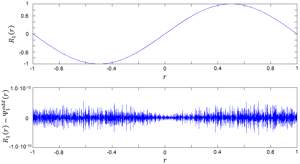
(b)
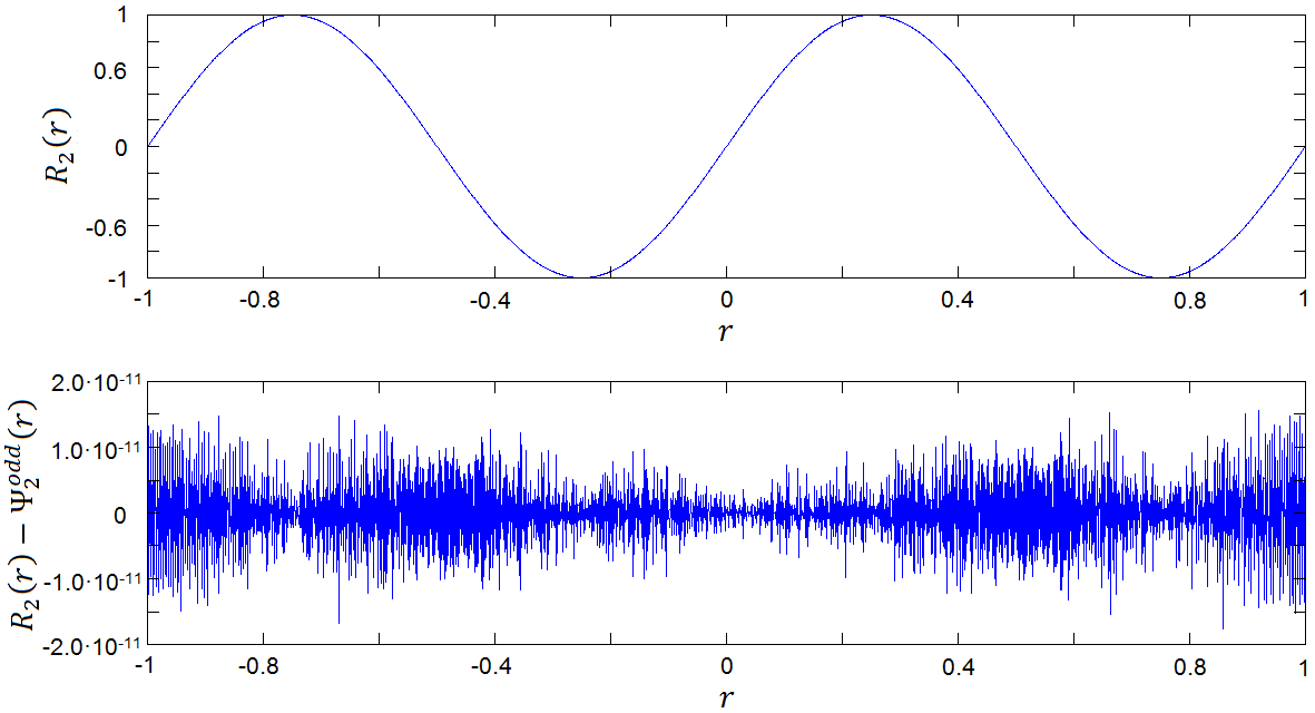
(c)

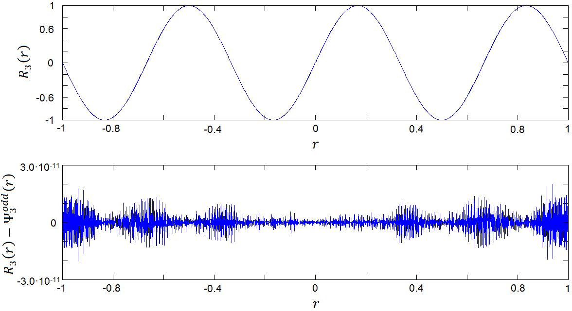
Figure 1: Graphical presentation of the first three odd eigenstates $R_{m}^{o}(r)=\sin(m\pi r/L)\,,~{}~{}m=1,2,3$, for $\beta=1.8$ and $L=1$, obtained by FFT. From the plots of $R_{m}^{o}(r)-\Psi_{m}^{odd}(r)\,,~{}m=1,2,3$, one can conclude that there is a very good agreement with the analytical eigenfunctions (10).

(a)
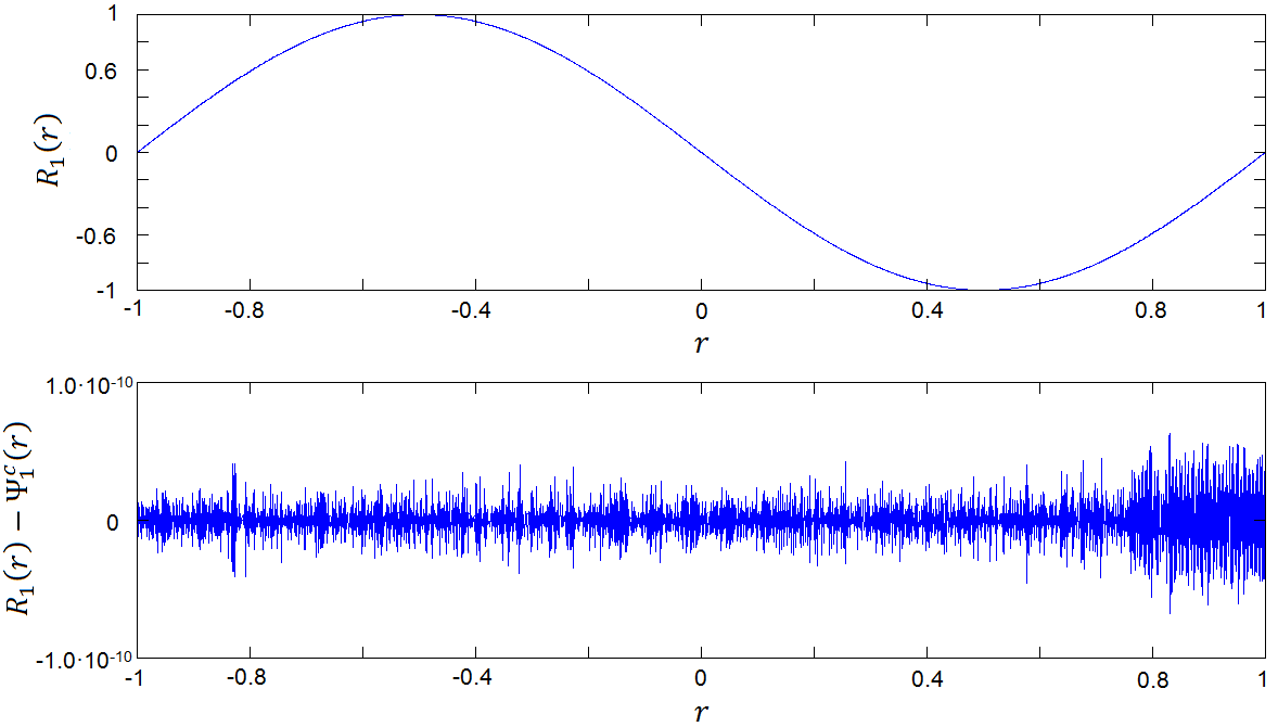
(b)
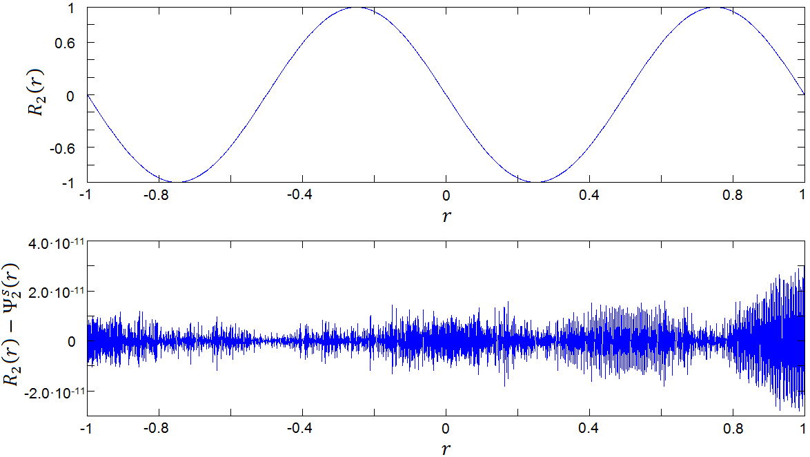
(c)
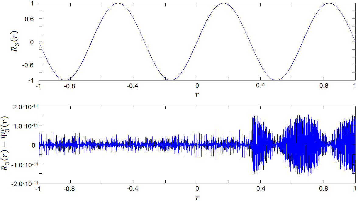
(d)

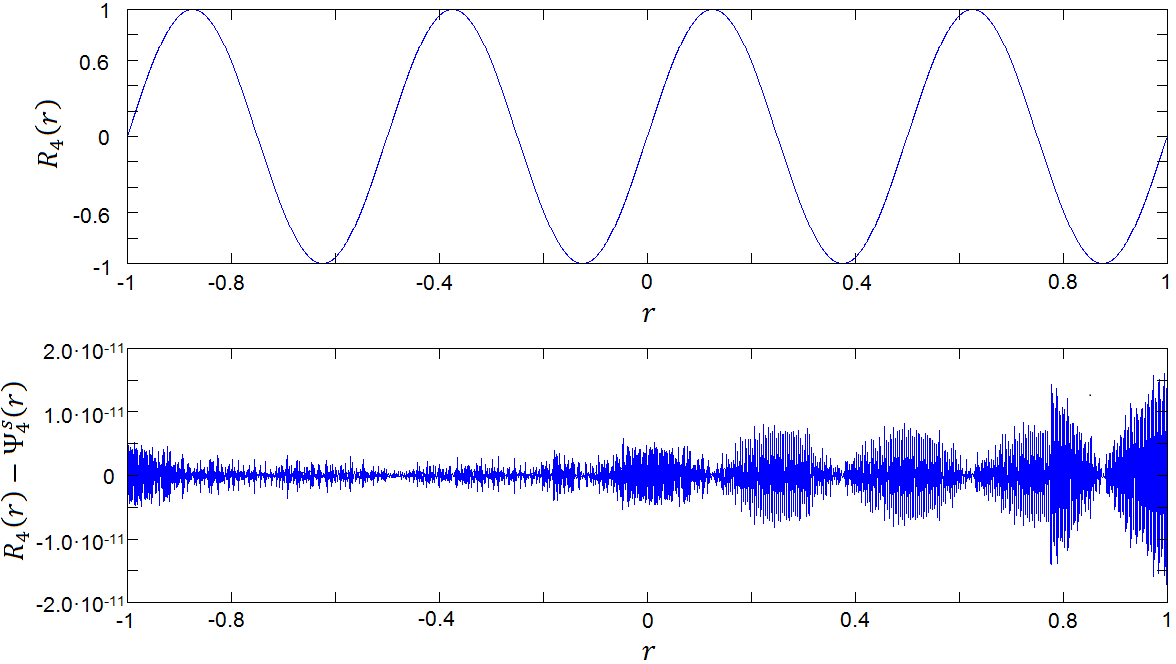
Figure 2: Graphical presentation of first fourth states for $\beta=1.8$ and $L=1$ for a class of degenerate functions with the spectrum $e_{m}=(\pi m/L)^{\beta}$, which corresponds to the odd eigenvalues. Here for each $m$, there are two normalized functions $\Psi_{m}^{c}(r)=\frac{1}{\sqrt{L}}\cos[m\pi(2r+L)/(2L)]$ and $\Psi_{m}^{s}(r)=\sin[m\pi(2r+L)/(2L)]$. However, the boundary conditions lift this degeneracy, such that for $m=2n$, one obtains $R_{m}(r)=\Psi_{m}^{s}(r)$, while for $m=2n+1$ one obtains $R_{m}(r)=\Psi_{m}^{c}(r)$.

V Summary

We concerned with fractional wave-diffusion processes, which take place in inhomogeneous composite media. We described them in the framework of a fractional Fokker-Planck equation (FFPE). A general form of the real-time-space FFPE (3) describes both waves and relaxation processes in a variety of applications of diffusion-wave phenomena in inhomogeneous media mainardi1 ; turski1 ; LevyLens ; mainardi ; Meerschaert ; mainardi2 ; nirD . The suggested scenario of the analysis is as follows. We started from a general form of the real-time-space FFPE, which however permits the variable separation. For the two-dimensional slab geometry, we developed a parabolic equation approximation which reduces the FFPE (3) to the space-time fractional Schrödinger equation (FSE). Then, since the obtained equation relates to a variety of quantum paradigms, one can employ the quantum mechanical terminology, noting that this use is formal only. The FSE (12) governs a Lévy transport in the slab geometry of inhomogeneous composite media, and in particular, it describes experimental realization of superdiffusive ray dynamics in Lévy glasses LevyLens and superdiffusion of ultra-cold atoms in an optical lattice nirD , where for these different processes, the Lévy walks are described by the same power law distribution $1/r^{1+\beta}$. For the space-time FSE (12), there is an effective time, which relates to the Caputo time fractional derivative and corresponds to the longitudinal direction of the real space of the slab geometry.

In the effective quantum dynamics according to the FSE, the Caputo fractional time derivative is responsible for the relaxation temporal behavior due to non-unitary evolution according the Mittag-Lefler functions in the solution (5). The transverse coordinates are responsible for the Lévy process by means of the Riesz fractional derivative in the infinite potential well, which is determined by the boundary conditions. This case of a “free Lévy” particle in the infinite potential well is described by Eq. (2) and it was analyzed numerically, and a correspondence of the numerical results with those obtained analytically in Ref. iomin_2015 is observed.

Regarding Eq. (2), few words are in order. As it is shown in iomin_2015 , the space fractional operator exists on the segment $[-L,L]$ only, and it corresponds to the quantum mechanics with a topological constraint. However, in addition to the introduction of fractional quantum mechanics by means of the Lévy-Feynman measure laskin1 , here the fractional quantum mechanics appears also as the result of the parabolic equation approximation in both space and time for the FFPE, which is specified by the finite boundary conditions. The introduction of the fractional operator of the kinetic energy in the infinite well potential on the scale $[-L,L]$ is natural, and any discussion about the wave function outside of this scale is irrelevant. As the result, the wave function can be periodically extended on the entire axis $(-\infty\,,\infty)$ that leads to the periodic solution, which is proven here numerically. We obtained graphical presentation of the odd eigenfunctions $R_{m}^{o}(r)=\frac{1}{\sqrt{L}}\sin\frac{m\pi r}{L}$ by using the fast Fourier transform (FFT) as a standard intrinsic function of the MATLAB package. It is worth noting that although this algorithm is not valid for the even eigenfunction, the obtained correspondence between analytical result and numerical, graphical calculations proves that the eigenfunctions of the Lévy flights in a box are periodic functions (see discussion in Ref. iomin_2015 ).

Appendix A Eigenvalue problem

In this appendix, we present a result obtained in Ref. iomin_2015 , where the eigenvalue problem of Eq. (2) has been considered for the fractional Laplace operator and the antisymmetric (odd) eigenfunctions $R_{e}^{\rm o}$ was found in the form

$$R_{e}^{\rm o}(x)=\Psi_{m}^{\rm odd}(x)=\frac{1}{\sqrt{L}}\sin\frac{m\pi x}{L}\,,~{}~{}~{}~{}m=1,2,\dots,$$ (A. 1)

which satisfies the boundary condition $\Psi_{m}^{\rm odd}(x=\pm L)=0$ and $x=r=\pm L$. We rewrite the fractional Laplace operator in the form (2), which is convenient in the analysis,

$$\hat{H}\Psi_{m}^{\rm odd}(x)=(i\partial_{x})\int_{-L}^{L}\left[\frac{1}{2\pi}\int_{-\infty}^{\infty}|k|^{\beta-2}ke^{-ik(x-y)}dk\right]\Psi_{m}^{\rm odd}(y)dy\,.$$ (A. 2)

Let us first perform integration over $y$. This yields

$$\frac{1}{2i}\int_{-L}^{L}\left[e^{iky+iz}-e^{iky-iz}\right]=(-1)^{m}\frac{2\pi m}{iL}\frac{\sin(kL)}{(k+z)(k-z)}\,,$$ (A. 3)

where $z=\pi my/L$. The next step is integration over $k$. From Eqs. (A. 2) and (A. 3), we have integrals

$$\frac{1}{2\pi}\int_{-\infty}^{\infty}\frac{k|k|^{\alpha-2}}{(k+z)(k-z)}\left[e^{ik(L-x)}-e^{-i(L+x)}\right]\equiv I^{(+)}-I^{(-)},$$ (A. 4)

where sign $(+)$ corresponds to the analytical continuation in the upper half plain, while $(-)$ corresponds to the analytical continuation in the lower half plain. Using the Residue theorem, one obtains that the integration yields

$$I^{(+)}-I^{(-)}=i(-1)^{m}\left(\frac{m\pi}{L}\right)^{\beta-2}\cos\left(\frac{m\pi}{L}x\right).$$ (A. 5)

Acting on this result by the rest part of the operator, which reads $(-1)^{m}\left(\frac{m\pi}{L}\right)(i\partial_{x})$, one obtains

$$\hat{H}\Psi_{m}^{\rm odd}(x)=\left(\frac{m\pi}{L}\right)^{\beta}\Psi_{m}^{\rm odd}(x)\equiv e_{m}^{\rm odd}\Psi_{m}^{\rm odd}(x).$$ (A. 6)

References

- (1) D. Kusnezov, A. Bulgac, G.D. Dang, Quantum Lévy Processes and Fractional Kinetics, Phys. Rev. Lett. 82: 1136, 1999.
- (2) N. Laskin, Fractals and quantum mechanics, Chaos 10: 780, 2000.
- (3) B.J. West, Quantum Lévy Propagators, J. Phys. Chem. B 104: 3830, 2000.
- (4) B.J. West, M. Bologna, P. Grigolini, Physics of Fractal Operators. Springer, New York, 2002.
- (5) J.-P. Bouchaud A. Georges, Anomalous Diffusion in Disordered Media: Statistical Mechanisms, Models and Physical Applications, Phys. Rep. 195: 127, 1990.
- (6) R. Metzler, J. Klafter, The random walk guide to anomalous diffusion: A fractional dynamics approach, Phys. Rep. 339: 1, 2000.
- (7) R.P. Feynman, A.R. Hibbs, Quantum Mechanics and Path Integrals. McGraw–Hill, New York, 1965.
- (8) M. Naber, Time fractional Schrodinger equation, J. Math. Phys. 45: 3339, 2004.
- (9) M.H. Stone, On one-parameter unitary groups in Hilbert Space, Ann. Math. 33: 643, 1932.
- (10) M. Kac, Probability and Related Topics in Physical Sciences. Interscience, NY, 1959.
- (11) L. Schulman, Techniques and applications of path integration. New York: Wiley; 1981.
- (12) M. Chaichian, A. Demichev, Path Integrals in Physics: Stochastic Process and Quantum Mechanics, Vol. 1 IOP Publishing, Bristol, 2001.
- (13) A. Iomin, Fractional-time quantum dynamics, Phys. Rev. E 80: 022103, 2009.
- (14) A. Iomin, Fractional-time Schrödinger equation: Fractional dynamics on a comb, Chaos, Solitons & Fractals 44: 348, 2011.
- (15) J.-N. Wu, C.-H. Huang, S.-C. Cheng, W.-F. Hsieh, Spontaneous emission from a two-level atom in anisotropic one-band photonic crystals: A fractional calculus approach, Phys. Rev. A 81: 023827, 2010.
- (16) M.A. Leontovich, On a method of solving the problem of propagation of electromagnetic waves along the earth’s surface, Proceedings of the Academy of Sciences of USSR, physics 8, 16 (1944) (in Russian).
- (17) R.V. Khokhlov, Wave propagation in nonlinear dispersive lines, Radiotekh. Elrctron. 6: 1116, 1961.
- (18) E.D. Tappert, The Parabolic Approximation Method, Lectures Notes in Physics, 70, in: Wave Propagation and Underwater Acoustics, eds. by J. B. Keller and J.S. Papadakis, Springer, New York, 224-287, 1977
- (19) L. Levi, Y. Krivolapov, S. Fishman, M. Segev, Hyper-transport of light and stochastic acceleration by evolving disorder, Nature Phys. 8: 912, (2012).
- (20) Y.Krivolapov, L. Levi, S. Fishman, M. Segev, M.Wilkinson, Super diffusion in optical realizations of Anderson localization, New J. Phys. 14: 043047, (2012).
- (21) L. Levi, M. Rechtsman, B. Freedman, T. Schwartz, O. Manela, M. Segev, Disorder-enhanced transport in photonic quasicrystals, Science 332: 1541, (2011).
- (22) M. Rechtsman, L. Levi, B. Freedman, T. Schwartz, O. Manela, M. Segev, Disorder enhanced transport in photonic lattices, Opt. Photon. News (Special Issue) 22: 33, (2011).
- (23) B.J. West, P. Grigolini, R. Metzler, T.F. Nonnenmacher, Fractional diffusion and Lévy stable processes, Phys. Rev. E 55: 99, 1997.
- (24) F. Mainardi, Fractional Calculus in Wave Propagation Problems, Forum der Berliner Mathematischer Gesellschaft 19: 20, 2011 (arXiv: [math-ph] 1202.0261).
- (25) B. Atamaniuk, A.J. Turski, Wave propagation and diffusive transition of oscillations in pair plasmas with dust, AIP Conf. Proc. 1041: 347, 2008.
- (26) P. Barthelemy, J. Bertolotti, D.S. Wiersma, A Lévy flight for light, Nature 453: 495 2008.
- (27) F. Mainardi, Fractional relaxation-oscillation and fractional diffusion-wave phenomena, Chaos, Solitons & Fractals 7: 1461, 1996.
- (28) M.M. Meerschaert, R.J. McGough, Attenuated fractional wave equations with anisotropy, J. Vibration and Acoustics 136: 051004, 2014.
- (29) J.M. Carcione, F. Cavallini, F. Mainardi, A. Hanyga, Time-domain modeling of constant-Q seismic waves using fractional derivatives, Pure Appl. Geophys. 159: 1719, (2002).
- (30) G. Casasanta, R. Garra, Fractional calculus approach to the acoustic wave propagation with space-dependent sound speed, Signal Image Video Processing 6: 389 2012.
- (31) I. Podlubny, Fractional Differential Equations (Academic Press, San Diego, 1999).
- (32) K.B. Oldham, J. Spanier, The Fractional Calculus Academic Press, Orlando, 1974.
- (33) S.G. Samko, A.A. Kilbas, O.I. Marichev, Fractional Integrals and Derivatives: Theory and Applications, Gordon and Breach, New York, 1993.
- (34) H. Bateman, A. Erdèlyi, Higher transcendental functions, vol. 3. New York: McGraw-Hill; 1955.
- (35) Y. Sagi, M. Brook, I. Almog, N. Davidson, Observation of anomalous diffusion and fractional self-similarity in one dimension, Phys. Rev. Lett. 108: 093002, 2012.
- (36) S. Marksteiner, K. Ellinger, P. Zoller, Anomalous diffusion and Le´vy walks in optical lattices, Phys. Rev. A 53: 3409, 1996.
- (37) D.A. Kessler, E. Barkai, Theory of fractional Lévy kinetics for cold atoms diffusing in optical lattices, Phys. Rev. Lett. 108: 230602, 2012.
- (38) A. Dechant, E. Lutz, D.A. Kessler, E. Barkai, Fluctuations of time averages for Langevin dynamics in a binding force field, Phys. Rev. Lett. 107: 240603, 2011.
- (39) R.K. Saxena, Z. Tomovski, T. Sandev, Fractional Helmholtz, fractional wave equations with Riesz-Feller and generalized Riemann-Liouville fractional derivatives, Eur. J. Pure Appl. Math. 7: 312, 2014.
- (40) R.K. Saxena, Ravi Saxena, S.L. Kalla, Computational solution of a fractional generalization of the Schrödinger equation occurring in quantum mechanics, App. Math. Comp. 216: 1412, (2010).
- (41) A. Iomin, Lévy flights in a box, Chaos, Solitons & Fractals 71: 73 (2015).