Trail-Needs pseudopotentials in quantum Monte Carlo calculations with plane-wave/blip basis sets

Abstract

We report a systematic analysis of the performance of a widely used set of Dirac-Fock pseudopotentials for quantum Monte Carlo (QMC) calculations. We study each atom in the periodic table from hydrogen ($Z=1$) to mercury ($Z=80$), with the exception of the $4f$ elements ($57\leq Z\leq 70$). We demonstrate that ghost states are a potentially serious problem when plane-wave basis sets are used in density functional theory (DFT) orbital-generation calculations, but that this problem can be almost entirely eliminated by choosing the $s$ channel to be local in the DFT calculation; the $d$ channel can then be chosen to be local in subsequent QMC calculations, which generally leads to more accurate results. We investigate the achievable energy variance per electron with different levels of trial wave function and we determine appropriate plane-wave cutoff energies for DFT calculations for each pseudopotential. We demonstrate that the so-called “T-move” scheme in diffusion Monte Carlo is essential for many elements. We investigate the optimal choice of spherical integration rule for pseudopotential projectors in QMC calculations. The information reported here will prove crucial in the planning and execution of QMC projects involving beyond-first-row elements.

I Introduction

Quantum Monte Carlo (QMC) methods are highly accurate, explicitly correlated wave-function-based techniques for calculating material properties from first-principles. The diffusion quantum Monte Carlo (DMC) methodCeperley and Alder (1980); Foulkes et al. (2001) is generally regarded as the most accurate first-principles method available for studying condensed matter. However, one significant weakness of DMC is its poor scaling with atomic number $Z$ in all-electron calculations. The computational expense of achieving a given statistical error bar scales as $O(Z^{5})$–$O(Z^{6.5})$.Hammond et al. (1994); Ceperley (1986); Ma et al. (2005) The physical origin of the problem is that the short length scale associated with core electrons (the Bohr radius of the hydrogen-like ion, which goes as $1/Z$) results in the need for very small time steps at large $Z$; on top of this there is the obvious additional expense due to the increase in the number of electrons with $Z$. In practice, it is usually only feasible to perform all-electron DMC calculations for first-row atoms. Furthermore, performing all-electron DMC calculations for anything beyond lithium generally requires the use of Gaussian or Slater-type basis sets rather than plane-wave basis sets to represent orbitals. For these reasons, the great majority of DMC studies of condensed matter have used pseudopotentials to represent atomic cores.Needs et al. (2010)

The use of nonlocal pseudopotentials introduces new difficulties, however. One issue is that the “standard” DMC algorithm assumes the potential-energy operator to be local. The most widely used solution to this difficulty is the pseudopotential locality approximation,Hurley and Christiansen (1987) in which the nonlocal pseudopotential $\hat{V}_{\rm NL}$ is replaced by $\Psi^{-1}\hat{V}_{\rm NL}\Psi$, where $\Psi$ is a trial wave function. This approximation leads to errors that are second order in the error in the trial wave function.Mitáš et al. (1991) Unfortunately these errors may be of either sign, undermining the variational principle for the fixed-node DMC ground-state energy.Foulkes et al. (2001) Furthermore, divergences in the localized pseudopotential due to nodes in the trial wave function can result in instabilities in the DMC algorithm. The latter two problems can largely be removed by means of a partial locality approximation known as the “T-move” scheme.Casula (2006); Casula et al. (2010) A more basic issue with the use of pseudopotentials is that they are generally constructed within the context of a single-particle method, such as Hartree-Fock theory or density functional theory (DFT). Only recently has the possibility of developing pseudopotentials for explicitly correlated many-body methods been explored.Trail and Needs (2013, 2015)

In this article we will examine a number of practical issues that affect the use of Dirac-Fock pseudopotentials in QMC calculations. In particular we will analyze the widely used Dirac-Fock pseudopotentials introduced by Trail and Needs, hereafter referred to as TN pseudopotentials.Trail and Needs (2005a, b) Most QMC calculations for real materials have featured either first- or second-row atoms.Needs et al. (2010) An issue that quickly emerges when one attempts to use TN pseudopotentials for transition metals “off the shelf” in plane-wave DFT orbital-generation calculations is the presence of ghost states due to the Kleinman-Bylander representation of the pseudopotentials in the DFT code.Kleinman and Bylander (1982) We demonstrate that this problem can generally be avoided in a straightforward fashion. We also investigate the energy variance per electron that can be achieved in QMC calculations for different elements, and we determine appropriate plane-wave cutoff energies for each pseudopotential. We have investigated various practical issues such as the optimal choice of spherical integration rule for pseudopotentials in QMC calculations.

The purpose of the present article is not to analyze the accuracy or otherwise of the TN pseudopotentials, but rather to determine how best to obtain consistent and precise QMC results using these pseudopotentials in conjunction with plane-wave basis sets. This is clearly a necessary first step towards assessing the accuracy of such calculations. It is of course also possible to use localized basis sets, such as Gaussian basis sets or Slater-type basis sets, in QMC calculations, with or without the use of pseudopotentials.

The rest of this article is arranged as follows. In Sec. II we describe the computational methodology that we have used to analyze the performance of TN pseudopotentials in QMC calculations. In Sec. III we present our results and analyze their implications for the use of pseudopotentials in QMC calculations. Finally we draw our conclusions in Sec. IV.

II Computational methodology

II.1 TN pseudopotentials

The TN pseudopotentials are Dirac-Fock average relativistic effective pseudopotentials optimized for QMC calculations.Trail and Needs (2005a, b) The core is as large as possible in each case, and pseudopotential data are provided for the $s$, $p$, and $d$ angular-momentum channels only. The issue of the need for higher-angular momentum channels in some cases is discussed in Ref. Tipton et al., 2014. Either $s$, $p$, or $d$ must be chosen to be the local channel, the potential for which is then applied to all higher angular-momentum components of the wave function. By default the $d$ angular-momentum channel is chosen to be local in the TN pseudopotentials. The other widely used set of Dirac-Fock pseudopotentials for QMC calculations is that proposed in Refs. Burkatzki et al., 2007 and Burkatzki et al., 2008. The performance of these two families of pseudopotentials in studies of small molecules is compared in Ref. Trail and Needs, 2014.

For each element we have taken the first TN pseudopotential listed in the library at https://vallico.net/casinoqmc/pplib/. This is a Dirac-Fock average relativistic effective pseudopotential tabulated on a radial grid. Core-polarization correctionsShirley and Martin (1993) are not used in this work. For many elements, alternative TN pseudopotentials are available. These are either constructed to be softer, or constructed using nonrelativistic Hartree-Fock theory; however, they are not considered in this work.

II.2 DFT calculations

The usual starting point for a QMC trial wave function is a Slater determinant of single-electron orbitals generated using DFT. We have performed plane-wave DFT calculations in order to determine whether or not each TN pseudopotential is affected by ghost states, and to generate trial wave functions for subsequent QMC calculations.

Our DFT orbital-generation calculations were performed using the castep plane-wave basis code.Clark et al. (2005) Each atom was placed in a simple cubic cell of side-length 15 bohr subject to periodic boundary conditions. The Perdew-Burke-Ernzerhof (PBE) generalized-gradient approximation exchange-correlation functionalPerdew et al. (1996) was used, and the plane-wave cutoff energy was 120 Ha in each case (except where the cutoff energy was varied to investigate convergence). We then performed spin-polarized calculations with the appropriate number of up- and down-spin electrons for the ground-state electronic configuration of the isolated atom.

In order to avoid ghost states we also performed PBE DFT calculations without a Kleinman-Bylander representation of the semilocal norm-conserving pseudopotentials. These calculations were performed with Gaussian basis functions using the molpro package.Werner et al. (2012, ) Large Gaussian basis sets were used, with aug-cc-pV5Z Dunning basis setsDunning (1989); Kendall et al. (1992); Peterson and Dunning (2002) used when available, and the pseudopotential equivalent used otherwise (for $39\leq Z\leq 54$ and $72\leq Z\leq 80$). All basis sets were uncontracted. Spin and orbital constraints were chosen in analog to the castep calculations, with the total spin constrained to be that of the ground-state configuration, and up- and down-spin orbitals unrestricted. For the Gaussian basis calculations we used the Gaussian expansion of each tabulated TN pseudopotential, available from the same source as the tabulated pseudopotentials.

Finite-basis errors for the Gaussian basis sets used in this work are expected to be small, but we have examined the issue in more detail for oxygen and copper. The convergence of the total energy with respect to basis-set index is expected to be rapid and exponential;Dunning (1989) hence the basis-set errors in the aug-cc-pV5Z results were estimated by three-point exponential extrapolation to the complete-basis-set limit using aug-cc-pV(T,Q,5)Z basis sets. This provides estimated basis-set errors of 0.002 and 0.005 Ha for oxygen and copper, respectively.

II.3 Trial wave functions

The plane-wave orbitals were re-represented in a blip (B-spline) basis.Alfè and Gillan (2004) This is faster to evaluate in a QMC calculation and allows us to dispense with the unwanted periodic boundary conditions on the isolated atoms and molecules studied in this work. For each orbital the grid of reciprocal-lattice points in the plane-wave expansion was padded out by a factor of three in each direction before a Fourier transformation to real space was carried out to obtain the blip representation of the orbital. We verified that this choice of “blip grid multiplicity” is sufficiently fine that the re-representation of the plane-wave orbitals in a blip basis has no statistically significant effects on our QMC results. We optimized three levels of correlated wave function: Slater-Jastrow (SJ) wave functions with isotropic electron-electron ($u$) and electron-nucleus ($\chi$) terms in the Jastrow factor; SJ wave functions with isotropic electron-electron ($u$), electron-nucleus ($\chi$), and electron-electron-nucleus ($f$) terms in the Jastrow factor;Drummond et al. (2004) and Slater-Jastrow-backflow (SJB) wave functions with isotropic electron-electron ($u$), electron-nucleus $(\chi$), and electron-electron-nucleus ($f$) terms in the Jastrow factor and isotropic electron-electron ($\eta$) and electron-nucleus ($\mu$) terms in the backflow function.López Ríos et al. (2006) In each case we used separate two-electron Jastrow and backflow terms for parallel- and antiparallel-spin electrons; where there were different numbers of up- and down-spin electrons we also used different two-electron Jastrow terms for up-up and down-down pairs. Likewise, for spin-polarized atoms, we used separate one-electron Jastrow and backflow terms for up- and down-spin electrons. The electron-electron-nucleus Jastrow terms were of the same form for all combinations of electron spins, however. For each atom the $u$, $\chi$, $f$, $\eta$, and $\mu$ functions were smoothly truncated at interparticle distances of 6, 6, 3, 6, and 6 bohr, respectively. The only SJB results we report are in our tests of DMC for a small-core copper atom, in Sec. III.4.1.

In our variational Monte Carlo (VMC) wave-function optimization calculations we used the unreweighted variance minimizationUmrigar et al. (1988); Drummond and Needs (2005) and energy minimizationNightingale and Melik-Alaverdian (2001); Toulouse and Umrigar (2007); Umrigar et al. (2007) methods. We used more than 10,000 electronic configurations in each optimization. We also performed QMC calculations using an uncorrelated product of Slater (S) determinants for up- and down-spin electrons.

II.4 DMC calculations

All our DMC calculations used time steps of $\delta\tau=0.0005$, 0.001, 0.002, and 0.004 Ha^-1, with the numbers of walkers being inversely proportional to $\delta\tau$ in each case. At small time steps the DMC time-step bias is linear in the time step while the finite-population bias is inversely proportional to the population;Umrigar et al. (1993) hence, linearly extrapolating our DMC energies to zero time step simultaneously removes the time-step and the population-control biases. We have performed DMC calculations with and without the T-move schemeCasula (2006); Casula et al. (2010) using Slater-Jastrow wave functions with electron-electron ($u$) and electron-nucleus ($\chi$) terms only in the Jastrow exponent.

III Results and discussion

III.1 Ghost states

Plane-wave DFT codes such as castep typically use the Kleinman-BylanderKleinman and Bylander (1982) form to represent pseudopotentials for reasons of efficiency. Unfortunately, for several elements, recasting the TN pseudopotentials in Kleinman-Bylander form results in the formation of so-called “ghost states” (spurious low-energy bound states).Gonze et al. (1990, 1991) The Kleinman-Bylander representation is slightly different to the semilocal representation of a pseudopotential, and the introduction of ghost states is not simply an artifact of basis-set incompleteness. The presence of ghost states gives rise to some or all of the following symptoms: the failure of the DFT self-consistent-field (SCF) process to converge; a large difference between the DFT energies obtained with plane-wave and Gaussian basis sets; the existence of an absurdly low Kohn-Sham eigenvalue; an absurdly high (unbound) energy when the orbitals are used in VMC calculations; a very large energy variance; enormous difficulty optimizing a trial wave function in VMC; and enormous difficulty controlling the configuration population in a DMC simulation. Furthermore, these difficulties may change or disappear when the local channel is changed.

In Fig. 1 we plot the difference between the DFT energy obtained using a plane-wave basis with a Kleinman-Bylander representation of the pseudopotential and the DFT energy obtained using a Gaussian basis for each TN pseudopotential. Choosing the $d$ channel to be local often leads to a relatively enormous difference between the plane-wave and Gaussian DFT results, strongly suggesting a problem caused by a ghost state. Choosing the $s$ channel to be local avoids this problem in every case apart from niobium. Choosing the $p$ channel to be local avoids the problem with ghost states in most cases. In Fig. 2 we indicate which TN pseudopotentials are likely to be affected by ghost states for different choices of local channel, based on this analysis of the DFT energies.

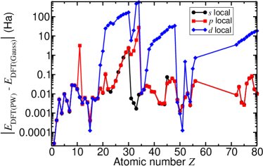
Figure 1: (Color online) Magnitude of difference between plane-wave and Gaussian DFT total energies $E_{\rm DFT(PW)}$ and $E_{\rm DFT(Gauss)}$ for each TN pseudopotential, for different choices of local channel. No results are given for lutetium because of the lack of availability of an accurate Gaussian basis set; this does not imply that lutetium is affected by ghost states. The DFT calculations for niobium with $s$ and $p$ local, vanadium, iron, and nickel with $p$ local, and manganese with $d$ local persistently failed to converge and are not shown in the graph.

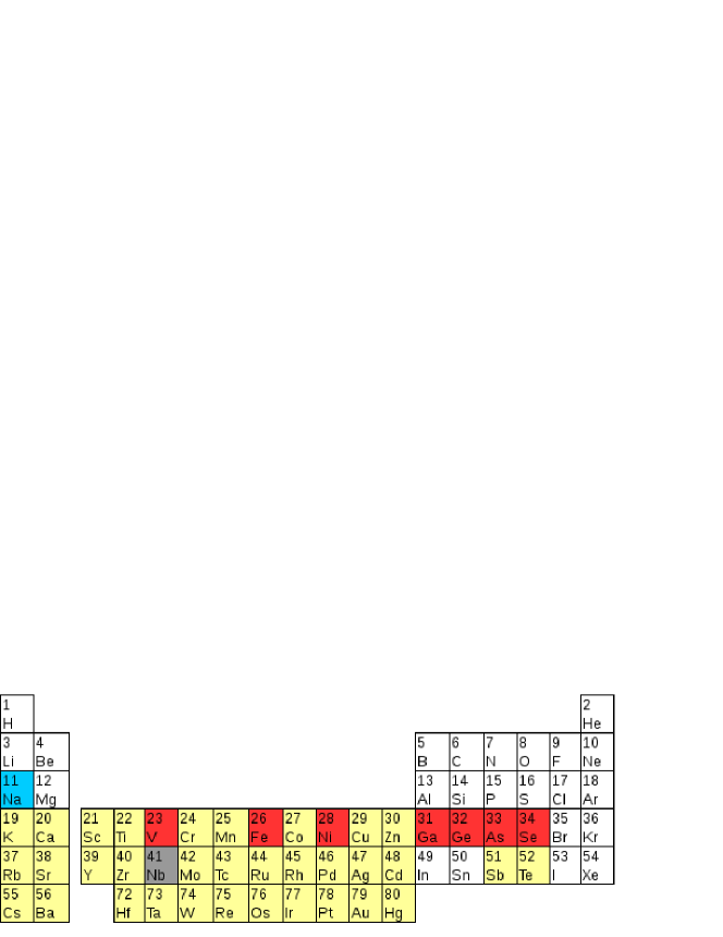
Figure 2: (Color online) TN pseudopotentials that are affected by ghost states for different choices of local channel in plane-wave DFT calculations. For elements in white cells, there are no ghost states; for elements in blue cells, choosing $p$ (but not $s$ or $d$) to be local results in ghost states; for elements in yellow cells, choosing $d$ (but not $s$ or $p$) to be local results in ghost states; for elements in red cells, choosing $p$ or $d$ (but not $s$) to be local leads to ghost states; and elements in grey cells are haunted by ghost states for any choice of local channel. Gaussian DFT results are not available for lutetium ($Z=71$), which is therefore omitted.

The set of Kohn-Sham eigenvalues obtained for the copper TN pseudopotential is shown in Table 1. Results are given for both Gaussian and plane-wave basis calculations, with the $s$ channel taken as local for the plane-wave calculations. In both cases the basis-set errors were estimated. The Gaussian basis-set eigenvalues were obtained by three-point exponential extrapolation to the complete-basis-set limit using aug-cc-pV(T,Q,5)Z basis sets, with errors estimated as the absolute difference between the extrapolated eigenvalues and those for the aug-cc-pV5Z basis set. The plane-wave basis-set eigenvalues were obtained by linear extrapolation with respect to $E_{\rm cut}^{-3/2}$, where $E_{\rm cut}$ is the plane-wave cutoff energy, using cutoff energies of $240$, $300$, and $360$ Ha. Errors were estimated as the absolute difference between the extrapolated values and those obtained for an energy cutoff of $360$ Ha. As suggested by Fig. 1, the largest error arises for the $d$-orbitals and plane-wave basis calculations. Total energies were obtained using the same extrapolation and error-estimation procedure. For the Gaussian and plane-wave basis sets the total energies were $-52.661(5)$ and $-52.49(1)$ Ha, respectively. The difference between them is significant, but sufficiently small that it can be ascribed to the Kleinman-Bylander representation with no ghost states present.

Table 1: Kohn-Sham eigenvalues for the occupied orbitals of the copper atom represented by a TN pseudopotential. The basis set is either Gaussian or plane-wave; a Kleinman-Bylander representation of the pseudopotential is used in the latter case. Estimated basis-set errors are shown in brackets.

		Eigenvalues (Ha)
Orbital	Basis	Spin-up		Spin-down
$4s$	Gaussian	$-0$.	$158987(4)$	$-0$.	$12136(6)$
$3d$	Gaussian	$-0$.	$262667(1)$	$-0$.	$258891(1)$
$4s$	Plane-wave	$-0$.	$1582(1)$	$-0$.	$1176(1)$
$3d$	Plane-wave	$-0$.	$2762(1)$	$-0$.	$2715(2)$

The presence of ghost states makes QMC work meaningless or impossible; however, inexperienced users may wrongly ascribe the problems encountered to the general difficulty of optimizing QMC trial wave functions. Eliminating ghost states from DFT orbital-generation calculations is a necessary but not sufficient condition for accurate QMC work. Even if the orbitals generated in the DFT calculation are unaffected by ghost states, the choice of local channel may still affect the behavior of the subsequent QMC calculations.

Figure 3 indicates which TN pseudopotentials are affected by ghost-state-like symptoms in QMC calculations using a plane-wave/blip basis for different choices of local channel (used in both the DFT and the subsequent QMC calculations). The criteria used for judging that a particular pseudopotential with a particular choice of local channel is problematic are the symptoms listed near the beginning of Sec. III.1. Only one TN pseudopotential, niobium, is apparently completely unusable in plane-wave calculations. The problem with niobium is not currently understood. In every other case, the problem of ghost-state-like symptoms can be avoided by choosing the $s$ channel to be local in the plane-wave DFT calculation.

We have verified that in QMC calculations that use orbitals generated with the $s$ channel chosen to be local, the local channel can either be left as $s$ or (preferably) changed to $d$; no symptoms of ghost states occur in either case. By contrast, there are several elements for which choosing the $p$ channel to be local does not cause any problems in the DFT calculation but does adversely affect the subsequent QMC calculations, as can be seen by comparing Figs. 2 and 3. Applying the potential for the $d$ channel to higher angular-momentum components in the QMC calculation is expected to be more accurate in principle than applying the potential for the $s$ channel; furthermore, as shown below, choosing $d$ to be local in QMC reduces the achievable variance in many cases.

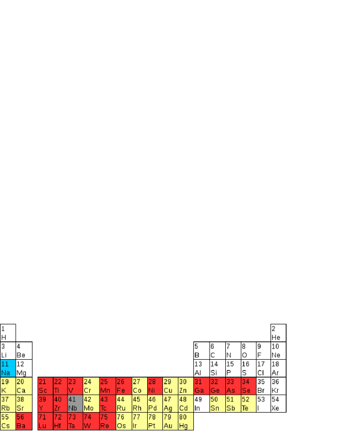
Figure 3: (Color online) TN pseudopotentials that are affected by ghost states or similar difficulties for different choices of local channel in QMC calculations using plane-wave DFT orbitals. For elements in white cells, there are no ghost-state-like symptoms; for elements in blue cells, choosing $p$ (but not $s$ or $d$) to be local results in ghost-state-like symptoms; for elements in yellow cells, choosing $d$ (but not $s$ or $p$) to be local results in ghost-state-like symptoms; for elements in red cells, choosing $p$ or $d$ (but not $s$) to be local leads to ghost-state-like symptoms; and elements in grey cells are affected by ghost-state-like symptoms for any choice of local channel.

Our previous experience with plane-wave DFT calculations for $3d$ transition metals suggests that choosing $p$ to be local provides reasonable energies, but is very vulnerable to unstable convergence and/or apparent convergence to different final energies for different initial conditions. A likely explanation for this behavior is a ghost state of similar energy to the actual state. This may well be the cause of the difference between the elements highlighted as being problematic when $p$ is local in Figs. 2 and 3. For the transition metal pseudopotentials the $s$ and $d$ characters of the wave functions are expected to be dominant near the nuclei, with the $p$ character being either minimal or zero. This suggests that taking $s$ rather than $p$ to be local in DFT calculations will be the most accurate choice, as it avoids an approximate projector representation for this channel.

III.2 Recommended plane-wave cutoff energies for TN pseudopotentials

We extrapolated the DFT energy of each pseudoatom to basis-set completeness by assuming the error scales as $E_{\rm cut}^{-3/2}$, where $E_{\rm cut}$ is the plane-wave cutoff energy (i.e., that the error falls off as the reciprocal of the number of plane waves). We used two cutoff values to perform the extrapolation (240 and 360 Ha, except where SCF convergence problems forced us to use smaller cutoffs). Having determined the basis-set-complete energy, we determined the plane-wave cutoff energy required to achieve a given basis-set error by linear interpolation in the DFT energy as a function of $E_{\rm cut}^{-3/2}$.

We have plotted the plane-wave cutoff energy required to achieve a given level of convergence in the DFT total energy against atomic number in Fig. 4. The cutoff energy required to converge the total energy of each atom to within so-called chemical accuracy (1 kcal mol^-1, which is 1.59 mHa) is shown, as is the cutoff energy required to converge the total energy to 0.1 mHa, an order of magnitude tighter than chemical accuracy. The required cutoff energies for the $3d$ transition metals are in many cases impractically large; hence any attempt to perform plane-wave-DFT-QMC calculations using the TN pseudopotentials for those atoms will inevitably encounter problems associated with large variances, and the outcome will at best rely on a cancellation of errors. An example of the sort of difficulties encountered for the $3d$ transition metals is given in Sec. III.4.1.

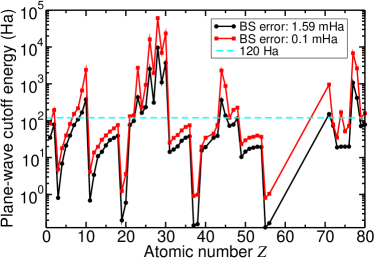
Figure 4: (Color online) Plane-wave cutoff energy required to achieve a given level of convergence in the DFT energy per atom for each TN pseudopotential. The $s$ channel is chosen to be local in each case. 120 Ha is the cutoff energy used for the tests reported in Fig. 7.

The dependence of the DMC energy on the orbitals in the Slater wave function is in general very weak, because the DMC energy only depends on the trial wave function via the fixed-node approximation and the pseudopotential locality approximation; however, the VMC energy, the VMC energy variance, and hence the efficiency of QMC calculations can depend significantly on the orbitals. It has been shownCeperley (1986) that, for a given wave-function form, the efficiency of the importance-sampled DMC algorithm is maximized when the trial wave function is optimized by energy minimization. Reducing the finite-basis error in the DFT total energy per atom provides a better starting point for optimization of the correlated part of the trial wave function, and the reduction in the DFT energy with increasing basis-set size translates directly into a reduction in the VMC energy, as shown for an oxygen atom in Fig. 5 and an oxygen molecule in Fig. 6. Since QMC calculations are generally intended to achieve chemical accuracy or higher, it is desirable for the finite-basis error in the DFT energy to be substantially less than chemical accuracy. Furthermore, as shown in Figs. 5 and 6, considerable reductions in the VMC variance can be achieved by increasing the plane-wave cutoff energy up to the value suggested by the convergence of the DFT total energy to chemical accuracy. The performance of unreweighted variance minimization improves significantly once the basis set becomes adequate. The results in Fig. 5 show that, apart from the lowest plane-wave cutoff energy studied, the DMC energy is almost independent of the cutoff energy.

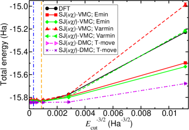
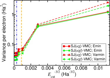
Figure 5: (Color online) Top panel: DFT, VMC, and DMC energies as a function of plane-wave cutoff energy $E_{\rm cut}$ for an isolated oxygen atom. Bottom panel: VMC energy variance against plane-wave cutoff energy for an isolated oxygen atom. Two different levels of correlated wave function were used in the VMC calculations, and energy minimization (“Emin”) and unreweighted variance minimization (“Varmin”) were used to optimize the wave functions. The dashed and dash-dotted vertical lines show the cutoff energies at which the DFT total energy is converged to within chemical accuracy and to within 0.1 mHa, respectively. The DMC calculations used the T-move scheme. Note that unreweighted variance minimization does not actually minimize the true variance of the energy; hence higher variances can be obtained with unreweighted variance minimization than with energy minimization.Drummond and Needs (2005)

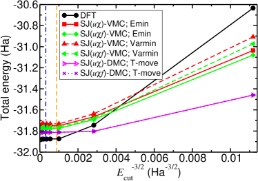
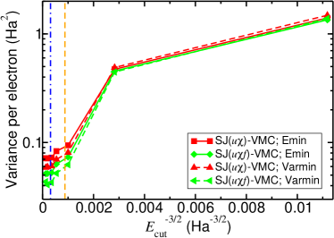
Figure 6: (Color online) As Fig. 5, but for an isolated oxygen molecule.

Comparing Figs. 5 and 6, it is clear that there is a significant cancellation of finite-basis errors in the VMC binding energy of an oxygen molecule, suggesting that one could “get away with” relatively low plane-wave cutoff energies. However, it is more efficient to use a high plane-wave cutoff energy (such that the DFT total energy is converged to 0.1 mHa), because it leads to an enormous reduction in the variance of the energies of the atom and the molecule, and hence gives smaller statistical error bars in the binding energy. When the orbitals are represented in a blip basis in QMC calculations, the cost of the calculation is only weakly dependent on the plane-wave cutoff energy. The cost of the DFT orbital-generation calculation clearly depends on the cutoff energy, but orbital generation is usually a negligibly small fraction of the computational expense of a QMC project.

We have investigated the extent to which it is important to use highly converged plane-wave orbitals in QMC calculations, i.e., whether it is crucial to use a tight tolerance for self-consistency in the orbital-generation DFT calculations. Although by construction the error in the DFT energy is second order in the error in the plane-wave coefficients, the error in the nodal surface (and hence the DMC energy) is first order in the error in the coefficients, albeit with a small prefactor. Similarly, the errors in the VMC energy and variance are first order in the error in the plane-wave coefficients. As can be seen in Table 2, there is no evidence of any need for tight SCF tolerances. That said, since DFT calculations are generally negligibly cheap compared with DMC calculations, there is no good reason for not using a tight convergence criterion.

Table 2: Effect of varying the SCF convergence tolerance in DFT orbital-generation calculations on subsequent VMC calculations for an isolated oxygen atom. The VMC calculations used Slater-Jastrow wave functions with $u$, $\chi$, and $f$ terms, which were optimized by energy minimization. The plane-wave cutoff energy was 200 Ha.

SCF tol. (Ha)	DFT en. (Ha)	VMC en. (Ha)	Var. per e. (Ha2)
$10^{-6}$	$-15.8371$	$-15.8353(4)$	$0$.	$042$
$10^{-7}$	$-15.8371$	$-15.8345(3)$	$0$.	$0392$
$10^{-8}$	$-15.8371$	$-15.8348(3)$	$0$.	$0388$
$10^{-9}$	$-15.8371$	$-15.8350(3)$	$0$.	$0385$
$10^{-10}$	$-15.8371$	$-15.8354(3)$	$0$.	$0382$
$10^{-11}$	$-15.8371$	$-15.8353(4)$	$0$.	$042$
$10^{-12}$	$-15.8371$	$-15.8355(3)$	$0$.	$0383$
$10^{-13}$	$-15.8371$	$-15.8348(3)$	$0$.	$0395$

III.3 Achievable energy variance with each TN pseudopotential

In Fig. 7 we plot the VMC energy variance achieved for each element using a fixed plane-wave cutoff energy of 120 Ha. Lower variances can nearly always be achieved by setting $s$ to be the local channel during the DFT orbital-generation calculation. The variance is either unchanged or lowered further if the $d$ channel is subsequently chosen to be local in the QMC calculation.

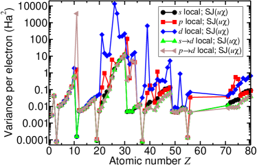
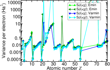
Figure 7: (Color online) Top panel: VMC energy variance per electron achieved with different angular-momentum channels chosen to be local (“$s\rightarrow d$” indicates that $s$ was chosen to be local in the DFT orbital-generation calculation, while $d$ was chosen to be local in the VMC calculation). We used the spin-polarized ground-state electronic configuration in each case. Energy minimization was used to optimize the trial wave function. Bottom panel: VMC energy variance per electron with the $s$ channel local in the DFT calculation and the $d$ channel local in the VMC calculation, using different levels of Slater-Jastrow trial wave function. Energy minimization (“Emin”) and unreweighted variance minimization (“Varmin”) were used to optimize the Jastrow factor in each case.

Once again it is clear that the most difficult cases by far are the $3d$ transition metals, where the variance is orders of magnitude larger than for other elements. Since the results shown in Fig. 7 were obtained using a fixed plane-wave cutoff energy of 120 Ha, this is partially due to the cutoff energy being too small, as shown in Sec. III.2. However, for real calculations, it becomes impractical to use the cutoffs required for these elements.

The lower panel of Fig. 7 shows that, although unreweighted variance minimization generally gives a lower variance than energy minimization, there are more cases in which variance minimization catastrophically fails.

III.4 Analysis of DMC total-energy calculations

III.4.1 Case study: copper atom

To investigate the feasibility of plane-wave-DFT-QMC calculations for $3d$ transition metals, we have carried out a series of calculations for an isolated copper atom using a small-core pseudopotential, in which the pseudocharge is 17. This is not one of the “standard” TN pseudopotentials, but is available via the TN pseudopotential library. In Fig. 8 we plot the DMC energy against time step for various choices of trial wave function and optimization method, with and without the use of T-moves.

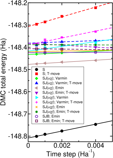
Figure 8: (Color online) DMC energy of a small-core copper pseudoatom against time step with different trial wave functions, with and without the use of T-moves. The trial wave functions were optimized by energy minimization (“Emin”) and unreweighted variance minimization (“Varmin”). The solid and dashed lines show fits to the data without and with T-moves, respectively. The orbitals were generated using a plane-wave cutoff energy of 120 Ha, and the $s$ channel was chosen to be local to avoid ghost-state problems.

It is clear that the choice of trial wave function and optimization method affects not only the behavior at finite time step, but also the final DMC energies extrapolated to zero time step. In all-electron fixed-node DMC calculations, the DMC energies at zero time step obtained using Slater and Slater-Jastrow wave functions are identical, because the nodal surface is not affected by the Jastrow factor. However, for copper, pseudopotential locality errors lead to differences on the scale of several eV between the DMC energies obtained with different Jastrow factors and without a Jastrow factor. This problem is significantly ameliorated by the use of the T-move scheme.

Table 3 shows the DMC energies in Fig. 8 extrapolated to zero time step and infinite population, together with the corresponding VMC energies and variances. Without T-moves the DMC energies depend significantly on the trial wave function and can be nonvariational. The spread of DMC energies is significantly reduced by the T-move scheme, and in particular the spuriously low energies obtained with poorer wave functions are eliminated. The change in the T-move DMC energy resulting from the inclusion of $f$ terms in the Jastrow factor is small compared with the difference in energy resulting from the inclusion of backflow. By contrast, including $f$ terms has a much larger effect on VMC energies than the inclusion of backflow. This suggests that, if one has a Slater-Jastrow wave function with $u$, $\chi$, and $f$ terms, locality errors are small compared with fixed-node errors. When the wave function is optimized by energy minimization, the standard error in the DMC energy is, as expected, significantly lower in general (this is always the case when T-moves are used). The energy variances per atom obtained with the small-core pseudopotential and reported in Table 3 are between one and two orders of magnitude smaller than the variances per atom obtained with the standard TN copper pseudopotential and reported in Fig. 7.

Table 3: DMC total energies in Fig. 8 extrapolated linearly to zero time step, together with VMC total energies and VMC energy variances per electron for an isolated small-core copper pseudoatom.

		DMC energy (Ha)				.		.
Wave fn.	Opt. meth.	Without T-moves		With T-moves		VMC energy (Ha)		Var. per elec. (Ha2)
Slater	N/A	$-148$.	$808(1)$	$-148$.	$3069(7)$	$-147$.	$653(9)$	$1$.	$6261$
SJ($u\chi$)	Varmin	$-148$.	$4329(4)$	$-148$.	$382(1)$	$-148$.	$158(4)$	$0$.	$2629$
SJ($u\chi$)	Emin	$-148$.	$4770(5)$	$-148$.	$3821(4)$	$-148$.	$196(4)$	$0$.	$3409$
SJ($u\chi f$)	Varmin	$-148$.	$418(3)$	$-148$.	$389(3)$	$-148$.	$032(3)$	$0$.	$1817$
SJ($u\chi f$)	Emin	$-148$.	$4200(2)$	$-148$.	$3884(2)$	$-148$.	$347(3)$	$0$.	$1837$
SJB	Emin	$-148$.	$425(1)$	$-148$.	$4064(4)$	$-148$.	$378(2)$	$0$.	$1167$

The copper atom is an extreme case that highlights a number of important issues: pseudopotential locality errors in the DMC total energy can be as large as several eV per atom, and they manifest themselves by significant dependence of the DMC energy on the Jastrow factor; pseudopotential locality errors can be greatly ameliorated by the use of the T-move scheme; if the plane-wave cutoff energy is smaller than ideal according to Fig. 4 then energy minimization appears to be more reliable than unreweighted variance minimization and also results in greater efficiency in subsequent DMC calculations; and including extra correlation in the trial wave function using, e.g., electron-electron-nucleus ($f$) terms reduces both locality errors and time-step bias.

Strategies that prevent numerical problems with copper can be expected to work for all the other transition metals, because copper has the deepest $d$ channel.

III.4.2 Population-control difficulties without T-move scheme

We have performed a series of DMC calculations for each TN pseudopotential with and without the T-move scheme, with the $s$ channel chosen to be local. The simulation parameters are described in Sec. II.4. When the T-move scheme was used, every single DMC calculation completed successfully; however, when the T-move scheme was not used population-control problems occurred for boron, carbon, oxygen, fluorine, and lutetium. It is perhaps surprising that all but one of these problem cases are first-row atoms.

III.5 Optimal choice of nonlocal integration grid

To apply a nonlocal pseudopotential operator to a generic trial wave function it is necessary to perform integrations over the surface of a sphere in order to project out the different angular-momentum components of the trial wave function. Seven different spherical integration rules are presented in Ref. Mitáš et al., 1991, and we refer to these as Rules 1–7. The number of grid points increases roughly as the square of the rule number, and each rule integrates an expansion in spherical harmonics $Y_{lm}$ up to $l=l_{\rm max}$ exactly, where $l_{\rm max}$ increases approximately linearly with rule number. In a QMC calculation the spherical grid is typically rotated randomly before each numerical integration, so that the numerical integrals are unbiased random estimates of the angular-momentum components of the trial wave function. Using an integration scheme with a small number of grid points has the obvious advantage of reducing the cost of each local-energy evaluation in a QMC calculation; on the other hand, using a smaller number of grid points increases the random error in the integration, and hence the standard error in the mean energy. It is therefore expected that there is an optimal numerical integration rule.

Two examples of the effects of using different nonlocal integration rules are reported in Tables 4 and 5, for an oxygen molecule and a monolayer of hexagonal indium selenide, respectively. For the oxygen molecule the most efficient integration rule is Rule 3, which uses six points and would be exact for an expansion in spherical harmonics up to $l_{\rm max}=3$. For indium selenide the optimal rule is Rule 2. However, since the efficiency falls off very much more steeply when the integration rule is too small than when it is too large, we recommend that Rule 4 be chosen to be the default. Rule 4 uses 12 points and would be exact for an expansion in spherical harmonics up to $l_{\rm max}=5$. Nevertheless, QMC practitioners should be aware of the possibility of substantially increasing the efficiency of their calculations by choosing Rule 3 instead of Rule 4.

Table 4: VMC total energy, variance per electron, and efficiency with different nonlocal pseudopotential integration rules for an isolated O₂ molecule. The efficiency is defined as the reciprocal of the product of the average walltime per iteration, the variance, and the mean decorrelation period. The calculations used a plane-wave cutoff energy of 120 Ha and a Slater-Jastrow trial wave function with electron-electron ($u$), electron-nucleus ($\chi$), and electron-electron-nucleus ($f$) terms, which was optimized by unreweighted variance minimization.

Rule	VMC en. (Ha)		Var. per e. (Ha2)		Effic. (Ha-2s-1)
1	$-31$	$.74(1)$	$86$	$.4$	$7$
2	$-31$	$.765(5)$	$12$	$.3$	$49$
3	$-31$	$.7646(5)$	$0$	$.077$	$5050$
4	$-31$	$.7649(4)$	$0$	$.059$	$4510$
5	$-31$	$.7649(4)$	$0$	$.059$	$3660$
6	$-31$	$.7649(4)$	$0$	$.059$	$2520$
7	$-31$	$.7649(4)$	$0$	$.059$	$1770$

Table 5: As Table 4 but for a $3\times 3$ simulation supercell of monolayer hexagonal indium selenide subject to periodic boundary conditions.

Rule	VMC en. (Ha)		Var. per e. (Ha2)		Effic. (Ha-2s-1)
1	$-22$	$.852(9)$	$1$	$.03$	$0$	$.09$
2	$-22$	$.870(1)$	$0$	$.0152$	$3$	$.91$
3	$-22$	$.869(1)$	$0$	$.0120$	$2$	$.80$
4	$-22$	$.870(1)$	$0$	$.0115$	$1$	$.95$
5	$-22$	$.870(1)$	$0$	$.0115$	$2$	$.12$
6	$-22$	$.870(1)$	$0$	$.0115$	$1$	$.62$
7	$-22$	$.870(1)$	$0$	$.0115$	$0$	$.94$

IV Conclusions

We have investigated various practical issues relating to the use of TN pseudopotentials in QMC calculations. In particular, we have determined the plane-wave cutoff energy required to converge the DFT energy per atom to a given level of accuracy for each atom in the periodic table up to mercury (with the exception of the lanthanides). We have shown that ghost states arising from the Kleinman-Bylander representation of pseudopotentials in plane-wave DFT calculations are a significant problem when the $p$ or $d$ channel is chosen to be local. We have shown that, in all cases apart from niobium, this problem can be avoided by choosing the $s$ channel to be local in the DFT calculation and the $d$ channel to be local in the subsequent QMC calculations.

We have investigated the achievable VMC energy variance with a Slater-Jastrow wave function for each TN pseudopotential. Our calculations demonstrate that accurate QMC calculations run off the back of plane-wave-pseudopotential DFT calculations for $3d$ elements, especially zinc and copper, cannot easily be achieved with TN pseudopotentials. The problematically large plane-wave basis sets required for the $3d$ transition-metal atoms seem to be a direct consequence of the norm-conserving pseudopotential generation process, so may not be easily controlled by modifying this generation process. We have shown that the T-move scheme significantly increases the reliability of DMC, and we recommend its use in general.