On SL(3,$\mathbb{C}$)-representations of the Whitehead link group

Abstract

We describe a family of representations in SL(3,$\mathbb{C}$) of the fundamental group $\pi$ of the Whitehead link complement. These representations are obtained by considering pairs of regular order three elements in SL(3,$\mathbb{C}$) and can be seen as factoring through a quotient of $\pi$ defined by a certain exceptional Dehn surgery on the Whitehead link. Our main result is that these representations form an algebraic component of the SL(3,$\mathbb{C}$)-character variety of $\pi$.

1 Introduction

Let $M$ be a manifold. The description of the character variety of $\pi_{1}(M)$ in a Lie group $G$ is closely related to the study of geometric structures on $M$ modelled on a $G$-space $X$. In this setting, representations of $\pi_{1}(M)$ into $G$ appear as holonomies of $(X,G)$-structures. In the case of a hyperbolic $3$-manifold $M$, a natural target group is PSL(2,$\mathbb{C}$) (or SL(2,$\mathbb{C}$)), as the holonomy of a hyperbolic structure on $M$ has image contained in PSL(2,$\mathbb{C}$). The study of these character varieties was initiated by Thurston, in the non-compact case, who described a natural way of constructing explicit representations of $\pi_{1}(M)$ in PSL(2,$\mathbb{C}$) using ideal triangulations of $M$ (see [Thu]). The rough idea is to parametrise hyperbolic ideal tetrahedra using cross-ratios, and to analyse the possible ways of constructing the hyperbolic structure on $M$ by gluing together these ideal tetrahedra. This method gives rise to a family of polynomial equations expressed in terms of a family of cross-ratios, which are often referred to as Thurston’s gluing equations (see Chapter 4 of [Thu]). The output of this method is a subvariety of $\mathbb{C}^{n}$ consisting of those tuples of parameters that satisfy Thurston’s equations, which is called the deformation variety. Representations can be expressed in terms of the cross-ratios, and one of the main interests of the deformation variety is that it allows explicit computations, which are very useful for experiments.

Thurston’s approach has been generalized for the higher dimensional target groups ${\mathrm{SL}}(n,\mathbb{C})$ in [BFG14, GTZ15, DGG13, GGZ15, Zic16]. This generalisation is geometrically meaningful. Indeed, the subgroups SU$(2,1)$ and ${\mathrm{SL}}(3,\mathbb{R})$ of ${\mathrm{SL}}(3,\mathbb{C})$ correspond respectively to spherical CR structures (see below) and real projective flag structures (see [FST15]), whereas ${\mathrm{SL}}(4,\mathbb{R})$ corresponds to projective structures on $3$-manifolds, well-studied in the convex case [Ben08]. The first examples following Thurston’s point of view for higher dimensional Lie groups were produced by Falbel in [Fal08], who constructed and studied examples of representations of the figure 8 knot group to SU(2,1) (see also [DF15, FW14]). A parallel is also to be drawn with higher Teichmüller theory in case of surfaces. In this note, we focus on the target group ${\mathrm{SL}}(3,\mathbb{C})$.

Though simple in spirit, this method of describing representation varieties becomes very involved when the number of tetrahedra grows. In fact, the only ${\mathrm{SL}}(3,\mathbb{C})$-character variety of a hyperbolic $3$-manifold that has been completely described so far with this approach is the one of the figure 8 knot complement [FGK⁺16], which admits an ideal triangulation by two tetrahedra (see Section 3.1 of [Thu]). Different methods have been used to describe examples of character varieties. In [HMP15], Heusener, Muñoz and Porti gave another description of the character variety of the figure 8 group starting directly from the group presentation. In [MP16], Munoz and Porti described character varieties for torus knots. We will consider here the example of the Whitehead link complement (which can be triangulated by 4 ideal simplices). Denote by $\pi$ its fundamental group. Denoting by $[x,y]=xyx^{-1}y^{-1}$ the commutator of $x$ and $y$, a possible presentation for $\pi$ is:

$$\langle x,y\,|\,[x,y][x,y^{-1}][x^{-1},y^{-1}][x^{-1},y]\rangle.$$

Let $\chi_{3}(\pi)$ be the corresponding ${\mathrm{SL}}(3,\mathbb{C})$-character variety, that is the GIT quotient

$$\chi_{3}(\pi)={\rm Hom}(\pi,{\mathrm{SL}}(3,\mathbb{C}))//{\mathrm{SL}}(3,\mathbb{C}).$$

The full computation of $\chi_{3}(\pi)$ is not achieved as of today and seems a difficult task. Our goal here is to describe an algebraic component of $\chi_{3}(\pi)$ that contains many examples of geometrically meaningful representations.

Our motivation comes from the study of the so-called spherical CR structures on hyperbolic 3-manifolds. These structures are examples of $(G,X)$-structures where $X$ is $\mathbf{S}^{3}$ and $G$ is PU(2,1). The holonomy of such a structure is thus a representation of $\pi_{1}(M)$ in PU(2,1). This motivates the study of representations of $\pi$ in $\textrm{SU}(2,1)$ which is a real form of SL(3,$\mathbb{C}$). Recall that PU$(2,1)$ is the group of holomorphic isometries of the complex hyperbolic plane $\mathbf{H}^{2}_{\mathbb{C}}$ and SU$(2,1)$ is a triple cover of it. The sphere $\mathbf{S}^{3}$ is the boundary at infinity of $\mathbf{H}^{2}_{\mathbb{C}}$. In particular, spherical CR structures arise naturally on the boundary at infinity of quotients of $\mathbf{H}^{2}_{\mathbb{C}}$ with non-empty region of discontinuity. Spherical CR structures can also be thought of as examples of projective flag structures on 3-manifolds on $M$, of which holonomies are representations of $\pi_{1}(M)$ to PSL(3,$\mathbb{C}$).

Striking examples of spherical CR structures have been produced by R. Schwartz in [Sch01, Sch07] about fifteen years ago. There, Schwartz described what is now called a spherical CR uniformisation of the Whitehead link complement, that is a spherical CR structure with the additional property that the holonomy representation has non-empty region of dicontinuity with quotient homeomorphic to the Whitehead link complement (see [Der15] for a precise definition). Since then, Deraux and Falbel [DF15] produced a spherical CR uniformisation of the complement of the figure eight knot, Deraux [Der] and Acosta [Aco15] deformed this uniformisation, Deraux [Der15] described a uniformisation of the manifold $m_{009}$, and Parker-Will [PW15] described another uniformisation of the Whitehead link complement, different from Schwartz’s one.

Our goal here is to provide a common frame for all these examples. The crucial remark is the following: the group $\pi$ has $\pi^{\prime}={\mathbb{Z}}_{3}*{\mathbb{Z}}_{3}$ as a quotient. Moreover, it has been observed that all the representations alluded to above have two features in common:

1. their sources are quotients of $\pi$ (hence these representations can be seen as representations of $\pi$)

2. these representations factor through $\pi^{\prime}$.

The second item can be rephrased by saying that the images of all these representations are subgroups of PU$(2,1)$ generated by a pair of regular order three elements (see the introduction of [PW15] for a list of groups generated by two regular order three elements that are known to be discrete and provide examples of spherical CR structures on various link complements).

We are going to prove that a component of the SL(3,$\mathbb{C}$)-character variety of $\pi$ is formed by representations that factor through $\pi^{\prime}$. Moreover this component contains all the representations mentionned above. Let us describe this component more precisely. Define $X_{0}$ as the subset of the character variety of $\pi^{\prime}$ corresponding to representations generated by two regular order three elements of ${\mathrm{SL}}(3,\mathbb{C})$ (recall that an order three element in ${\mathrm{SL}}(3,\mathbb{C})$ is regular if and only if its trace is $0$). Our main result is the following.

Theorem 1.

The character variety $\chi_{3}(\pi)$ contains $X_{0}$ as an algebraic component of dimension $4$. In particular, all representation classes in this component are unfaithful.

The unfaithfulness part of Theorem 1 is straightforward once noted that all representation in $X_{0}$ factor through $\pi^{\prime}$.

The ${\mathrm{SL}}(2,\mathbb{C})$-character variety $\chi_{2}(\pi)$ for $\pi$ has been computed in [BC16]. It has two components: one contains the characters of every irreducible representations ; the other component contains the characters of every reducible representations. Using the irreducible representation ${\mathrm{SL}}(2,\mathbb{C})\to{\mathrm{SL}}(3,\mathbb{C})$, we get a natural map $\chi_{2}(\pi)\to\chi_{3}(\pi)$. Our component $X_{0}$ of $\chi_{3}(\pi)$ is new, in the sense that it does not contain the image of any component of $\chi_{2}(\pi)$. Indeed, a generic point in either component of $\chi_{2}(\pi)$, as described in [BC16], does not correspond to a representation of $\pi^{\prime}$.

It should be noted that the group $\pi^{\prime}$ is the fundamental group of a compact exceptional Dehn filling of the Whitehead link complement, as we will see later on. The situation we describe is therefore very similar to the one of the SL(3,$\mathbb{C}$) character variety of the figure $8$-knot group (see [HMP15, Proposition 10.3] or [FGK⁺16, Section 5.3]). There, a $2$-dimensional component of the character variety is formed by representations factoring through a quotient of $\pi^{\prime}$, which can be viewed as the fundamental group of a non-hyperbolic Dehn surgery on the figure $8$-knot complement. This quotient is isomorphic to an index 2 subgroup of the $(3,3,4)$-triangle group, which is in turn a quotient of $\pi^{\prime}$. As such (see Proposition 4), the aforementioned $2$-dimensional component for the $8$-knot complement may be seen as a slice of the $4$-dimensional component for the Whitehead link complement described in Theorem 1.

The proof of Theorem 1 has two steps.

• First we prove that $X_{0}$ is a closed Zariski subset in $\chi_{3}(\pi)$ and has dimension at least $4$ (see Proposition 7).

• Secondly we consider the particular point of $X_{0}$ associated to a representation $\rho_{0}$ and show that the dimension of the Zariski tangent space to $\chi_{3}(\pi)$ at this point is also $4$ (see Proposition 8). As a consequence, the dimension of the complex algebraic variety $X_{0}$ is at most $4$. The representation $\rho_{0}$ is defined in Section 3.4. It has been analysed geometrically in [PW15] and corresponds to a spherical CR uniformisation of the Whitehead link complement.

The main technical part in our work is the proof of Proposition 8. We choose to prove this proposition using a method that is not specific to the Whitehead link complement, and we believe that it could be used to study further examples. It involves the so-called deformation variety as described in [FGK⁺16]. The latter is an affine algebraic set, which is – at least around $[\rho_{0}]$ – a ramified covering of the character variety. The purpose of shifting to the deformation variety is that it allows effective computations via decorated representations and triangulations, as in [FGK⁺16].

In the last section, we describe an explicit family of pairwise unconjugate representations of $\pi^{\prime}$, whose conjugacy classes form a Zariski open subset of $X_{0}$. Our motivation for describing this generic set of actual matrices in the component $X_{0}$ is that this component should provide a nice playground for experimentations with the geometric structures we mentionned above. Having explicit expressions is very useful for that. This is called, in the works of Culler, Morgan and Shalen [CS83, MS84] a tautological representation of $X_{0}$ [CS83, MS84]. These representations are defined by pairs of regular order three matrices $(A,B)$ with no common eigenvector that are parametrised by the traces of the four products $AB$, $A^{-1}B$, $A^{-1}B^{-1}$ and $AB^{-1}$. These parameters are natural coordinates on $X_{0}$, in view of Lawton’s description of the character variety of the rank $2$ free group given in Theorem 6 (see [Law07]).

This paper is organised as follows. In Section 2, we describe the Whitehead link complement and its fundamental group from the perspective of (real) hyperbolic geometry. In particular, we gather together classical information on presentations and parabolic subgroups of $\pi$ that will be needed further. Section 3 is devoted to the character variety of $\pi$. We provide basic definitions and facts on these objects. We prove Proposition 7, state Proposition 8 and derive Theorem 1 from them. In Section 4, we present the deformation variety and prove Proposition 8. Eventually, in Section 5, we describe an explicit parametrisation of the representations in $X_{0}$. The interested reader may also want to use the companion Sage notebook [Gui] which combines the use of SnapPy [CDW] and SageMath [Dev16] to illustrate our method.

Aknowledgement: We wish to thank Miguel Acosta, Martin Deraux, Elisha Falbel, Michael Heusener and John Parker for numerous stimulating conversations. We thank Neil Hofmann, Craig Hodgson, Bruno Martelli and Carlo Petronio for kindly answering our questions.

2 Hyperbolic geometry of the Whitehead Link Complement

The Whitehead link is depicted on Figure 1. We denote by $W$ its complement in $\mathbf{S}^{3}$ and by $\pi$ the fundamental group of $W$.

2.1 The ideal octahedron

It is a well-known fact that $W$ carries a (unique) complete hyperbolic structure (we refer to [Thu] for more details). This structure can be explicitly described by considering an ideal regular octahedron in the real hyperbolic $3$-space ( see Figure 1), together with identifications of its faces by isometries. We refer the reader to Section 3.3 of [Thu], or to Example 1 in [Wie78] for details. We briefly recall here the description of this structure which is given in [Wie78].

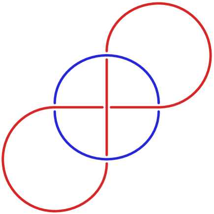
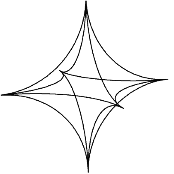
Figure 1: The Whitehead link, and a hyperbolic regular ideal octahedron.

We denote by $\mathcal{O}$ the ideal octahedron of which vertices are given, in the upper half-space model of $\mathbf{H}^{3}_{\mathbb{R}}$ by

$$\infty,\,0,\,-1,\,-1+i,\,i,\,\dfrac{-1+i}{2}.$$

A flattened version of this octahedron is pictured in Figure 2. We denote by $x$, $y$ and $t$ the isometries of $\mathbf{H}^{3}_{\mathbb{R}}$ associated to the following elements of SL(2,$\mathbb{C}$).

$$x=\begin{bmatrix}1&i\\ {\color[rgb]{0,0,0}0}&1\end{bmatrix},\,t=\begin{bmatrix}1&2\\ {\color[rgb]{0,0,0}0}&1\end{bmatrix}{\rm and}\,y=\begin{bmatrix}1&{\color[rgb]{0,0,0}0}\\ -1-i&1\end{bmatrix}.$$ (1)

In Wielenberg’s article, $x$ corresponds to $u$, $t$ to $t_{2}$ and $y$ to $w_{1}$. Let $\Gamma$ be the subgroup of PSL(2,$\mathbb{C}$) generated by $x$ and $y$.

Note that $t$ belongs to $\Gamma$ since $t=[y^{-1},x][y,x]x^{2}$. Now, we equip $\mathcal{O}$ with the face identifications described on Figure 2. This particular choice gives a holonomy representation with image $\Gamma$, which is isomorphic to the fundamental group of the Whitehead link complement, and can be seen to have index twelve in the Bianchi group PSL(2,${\mathbb{Z}}[i]$) (see [Wie78]). The octahedron from Figure 2 is a fundamental domain for $\Gamma$, and applying Poincaré’s polyhedron theorem leads to the following classical presentation for $\pi$.

$$\langle x,y\,|\,[x,y][x,y^{-1}][x^{-1},y^{-1}][x^{-1},y]\rangle.$$ (2)

We refer the reader to chapter 11 of [Rat06] for an exposition of Poincaré’s polyhedron theorem

$\alpha=yx^{-1}$ : $A\longmapsto A^{\prime}$ $\beta=yx^{-1}y^{-1}$ : $B\longmapsto B^{\prime}$ $\gamma=t^{-1}xy^{-1}$ : $C\longmapsto C^{\prime}$ $\delta=x^{-1}$ : $D\longmapsto D^{\prime}$,

Figure 2: An octahedron with face identifications

2.2 Triangulating the ideal octahedron

The presentation of the Whitehead link group that we are going to use is in fact not (2), but

$$\langle a,b|[ba^{-3}b^{2},a^{-1}b]\rangle.$$ (3)

An isomorphism between the two presentations is given by the changes of generators

$$(x,y)=(ab^{-1},ab^{-1}a)\mbox{ and }(a,b)=(x^{-1}y,x^{-2}y).$$ (4)

This isomorphism appears in [PW15] (Proposition 3.3), where it has a geometric meaning. The presentation (3) is the one provided by the software SnapPy [CDW]. It is worth noting that the computation made by SnapPy is based on an ideal triangulation of the Whitehead link complement, which is going to be of use for us, and is as follows. Connect the vertices with coordinates $\infty$ and $\frac{-1+i}{2}$ by an edge. One obtains a decomposition of the octahedron $\mathcal{O}$ as a union of four ideal tetrahedra, which we label as follows (see Figure 2).

$$\begin{array}[]{ll}\Delta_{0}=\Bigl{(}i,0,\dfrac{-1+i}{2},\infty\Bigr{)}&\Delta_{1}=\Bigl{(}-1+i,i,\dfrac{-1+i}{2},\infty\Bigr{)}\\ &\\ \Delta_{2}=\Bigl{(}-i,-1+i,\dfrac{-1+i}{2},\infty\Bigr{)}&\Delta_{3}=\Bigl{(}0,-i,\dfrac{-1+i}{2},\infty\Bigr{)}\end{array}$$ (5)

The geometric representation of $\pi$ is defined (up to PSL(2,$\mathbb{C}$)-conjugation) as the one corresponding to the unique finite volume hyperbolic structure on the Whitehead link complement. We denote it by $\rho_{\rm geom}$. It can be described in terms of either presentations (2) or (3). We now provide matrices for the images of $a$ and $b$ in the presentation (3) that can be easily related to (2) by the isomorphism (4).

Proposition 2.

The geometric representation of $\pi$ is the morphism $\rho_{\rm geom}:\pi\longrightarrow{\rm PSL}(2,\mathbb{C})$ defined by

$$\rho_{\rm geom}(a)=x^{-1}y=\begin{bmatrix}i&-i\\ -1-i&1\end{bmatrix}\mbox{ and }\rho_{\rm geom}(b)=x^{-2}y=\begin{bmatrix}-1+2i&-2i\\ -1-i&1\end{bmatrix}.$$ (6)

The geometric representation is thus a discrete and faithful representation of $\pi$ in PSL(2,$\mathbb{C}$) with image $\Gamma$. Note that $\rho(b^{-1}a^{3}b^{-1}a^{-1})=t$.

2.3 Stabilizers of the vertices and peripheral curves

There are two orbits of vertices modulo the identifications in the octahedron $\mathcal{O}$: the one of $\infty$ and the one of $0$. It is a simple exercise using the face identifications to verify that the stabilizers of these two points are respectively $\Gamma_{\infty}=\langle x,t\rangle$, and $\Gamma_{0}=\langle y,xy^{-1}xt^{-1}x^{-1}y^{-1}x\rangle$. The second generator for $\Gamma_{0}$ is the projective transformation associated to

$$\begin{bmatrix}1&{\color[rgb]{0,0,0}0}&\\ 2-2i&1\end{bmatrix}.$$

We express now these stabilizers in terms of $a$ and $b$.

Proposition 3.

The stabilizers of $0$ and $\infty$ in $\Gamma$ are the images of the two subgroups of $\pi$ respectively given by $\langle ab^{-1}a,s_{0}\rangle$ and $\langle ab^{-1},s_{\infty}\rangle$ by $\rho_{geom}$, where $s_{0}=[a,b^{-1}]a^{-1}b^{2}a^{-3}[b,a]$ and $s_{\infty}=b^{-1}a^{3}b^{-1}a^{-1}$.

Remark 1.

SnapPy provides the following generators for the first homology group of the boundary tori of the Whitehead link complement using the presentation (3) ($m_{i}$ stands for meridian, and $l_{i}$ for longitude):

$$m_{1}=a^{-2}b,\,l_{1}=a^{-2}bab^{-2}ab,\,m_{2}=b^{-1}a,\,l_{2}=b^{-1}ab^{-1}aba^{-3}ba.$$ (7)

By a direct computation, one verifies that

$$\rho_{\rm geom}(am_{1}a^{-1})=y \rho_{\rm geom}(al_{1}a^{-1})=y^{-2}s_{0}$$

$$\rho_{\rm geom}(am_{2}a^{-1})=x \rho_{\rm geom}(al_{2}a^{-1})=t^{-1}x^{2}$$

We see therefore that $m_{1}$ and $l_{1}$ correspond to the cusp of $W$ associated to (the orbit of) $0$, and that $m_{2}$ and $l_{2}$ correspond to the one associated to (the orbit of) $\infty$.

3 The SL(3,$\mathbb{C}$)-character variety

3.1 Generalities

Definition 1.

Let $G$ be a finitely generated group. The representation variety of $G$ in SL(3,$\mathbb{C}$) is

$${\rm Hom}(G,{\rm SL}(3,\mathbb{C})).$$

Its GIT quotient

$${\rm Hom}(G,{\rm SL}(3,\mathbb{C}))//{\rm SL}(3,\mathbb{C}),$$

where the action is by conjugation of representations, is called the SL(3,$\mathbb{C}$)-character variety, denoted by $\chi_{3}(G)$.

We refer the reader to [Sik12, Heu16] for classical definitions about representation and character varieties and associated objects. A remark is important for our purposes: if $G^{\prime}$ is a quotient of $G$, then there is a natural map:

$$\mbox{\rm Hom}(G^{\prime},{\rm SL}(3,\mathbb{C}))\hookrightarrow\mbox{\rm Hom}(G,{\rm SL}(3,\mathbb{C})).$$

Indeed, a representation $\rho^{\prime}:G^{\prime}\to{\rm SL}(3,\mathbb{C})$ is naturally promoted to a representation

$$\rho:G\twoheadrightarrow G^{\prime}\xrightarrow{\rho^{\prime}}{\rm SL}(3,\mathbb{C}).$$

As the projection $G\twoheadrightarrow G^{\prime}$ is surjective, this map is injective and moreover two representation $\rho^{\prime}$ and $\bar{\rho}^{\prime}$ in $\mbox{\rm Hom}(G^{\prime},{\rm SL}(3,\mathbb{C}))$ are conjugate if and only if their associated $\rho$ and $\bar{\rho}$ in $\mbox{\rm Hom}(G,{\rm SL}(3,\mathbb{C}))$ are conjugate. From Proposition 1.7 in [LM85], the map on the level of representation variety is a closed immersion covariant for the action of PGL(3,$\mathbb{C}$) by conjugation. From the discussion in page 15 of [LM85], this map induces a closed immersion on the level of character varieties. We obtain therefore

Proposition 4.

If $G^{\prime}$ is a quotient of $G$, then $\chi_{3}(G^{\prime})\subset\chi_{3}(G)$.

3.2 A quotient of $\pi$

We denote by $\pi^{\prime}$ the quotient of $\pi$ defined by the extra relations $a^{3}=b^{3}=1$. More precisely, a presentation for $\pi^{\prime}$ is given by $\pi^{\prime}=\langle a,b|a^{3},b^{3},[ba^{-3}b^{2},a^{-1}b]\rangle$. Clearly, the group $\pi^{\prime}$ is isomorphic to ${\mathbb{Z}}_{3}\star{\mathbb{Z}}_{3}$: the last relation is a consequence of the first two. Moreover, SnapPy indicates that $\pi^{\prime}$ is the fundamental group of a double Dehn surgery on the Whitehead link. We make this statement precise as follows.

Proposition 5.

The group $\pi^{\prime}\simeq{\mathbb{Z}}_{3}\star{\mathbb{Z}}_{3}$ is isomorphic to the quotient of $\pi$ defined by the two relations $m_{1}^{3}l_{1}^{-1}$ and $m_{2}^{3}l_{2}^{-1}$.

The proof of Proposition 5 is a direct verification from the definition of $l_{i}$ and $m_{i}$ given in Remark 1: the two conditions $m_{1}^{3}l_{1}^{-1}=m_{2}^{3}l_{2}^{-1}=1$ imply that $a^{3}=b^{3}=1$. In terms of Dehn surgery, $\pi^{\prime}$ is the fundamental group of the double Dehn surgery of slopes $(-3,-3)$ on the Whitehead link. This double Dehn surgery is not hyperbolic: this may be verified using SnapPy (see the companion Sage notebook to this paper [Gui]). More precisely, it can be seen to be the connected sum of two lens spaces (see [MP06, Table 2]).

3.3 A lower bound for $\dim(X_{0})$

We are now going to describe the SL(3,$\mathbb{C}$)-character variety of $\pi^{\prime}$. To this end, we use Lawton’s theorem on the SL(3,$\mathbb{C}$)-character variety of the rank two free group $F_{2}$ [Law07].

Theorem 6 (Lawton [Law07]).

The map $\psi$ defined by

$$\begin{array}[]{ccl}{\mathrm{SL}}(3,\mathbb{C})\times{\mathrm{SL}}(3,\mathbb{C})&\rightarrow&\mathbb{C}^{8}\\ (A,B)&\mapsto&(\mbox{\rm tr}A,\mbox{\rm tr}B,\mbox{\rm tr}AB,\mbox{\rm tr}A^{-1}B,\mbox{\rm tr}A^{-1},\mbox{\rm tr}B^{-1},\mbox{\rm tr}A^{-1}B^{-1},\mbox{\rm tr}AB^{-1})\end{array}$$

is onto $\mathbb{C}^{8}$ and descends to a (double) branched cover $\underline{\psi}:\chi_{3}(F_{2})\longrightarrow\mathbb{C}^{8}$.

The theorem in Lawton’s work is more precise and gives an explicit polynomial in $9$ variables defining $\chi_{3}(F_{2})$ as a hypersurface in $\mathbb{C}^{9}$ covering $\mathbb{C}^{8}$. Namely, the above double cover corresponds to the fact that the traces of the nine words $A$, $B$, $AB$, $A^{-1}B$, $A^{-1}$, $B^{-1}$, $A^{-1}B^{-1}$, $AB^{-1}$ and $[A,B]$ satisfy a relation of the form

$$(\mbox{\rm tr}[A,B])^{2}-S\cdot\mbox{\rm tr}[A,B]+P=0,$$ (8)

where $S$ and $P$ are polynomials in the traces of the first eight above words. In other words, once the traces of $A$, $B$, $AB$, $A^{-1}B$, $A^{-1}$, $B^{-1}$, $A^{-1}B^{-1}$, $AB^{-1}$ are fixed, the trace of $[A,B]$ is determined up to the choice of a root of (8). We provide the precise values of $S$ and $P$ in the last section of the Sage notebook [Gui], they may also be found in Lawton’s [Law07], or in [Wil16].

We can now give an alternate definition of the set $X_{0}$ considered in the introduction:

Definition 2.

Let $X_{0}\subset\chi_{3}(F_{2})$ be the inverse image by $\underline{\psi}$ of the subspace $V$ of $\mathbb{C}^{8}$ given by

$$V=\{(0,0,z_{1},z_{2},0,0,z_{3},z_{4}),z_{i}\in\mathbb{C}\}.$$

By Proposition 4, the sequence of quotients $F_{2}\twoheadrightarrow\pi\twoheadrightarrow\pi^{\prime}$ gives rise to a sequence of inclusions:

$$\chi_{3}(\pi^{\prime})\subset\chi_{3}(\pi)\subset\chi_{3}(F_{2}).$$

With these inclusions in mind, we see that $X_{0}$ is actually included in $\chi_{3}(\pi^{\prime})$. We can even be more specific:

Proposition 7.

The set $X_{0}$ is an irreducible Zariski closed subset of $\chi_{3}(\pi^{\prime})$. Its dimension is at least $4$.

Proof.

First, $X_{0}$ is included in $\chi_{3}(\pi^{\prime})$. Indeed, the condition $\psi(A,B)\in V$ rewrites

$$\mbox{\rm tr}A=\mbox{\rm tr}A^{-1}=\mbox{\rm tr}B=\mbox{\rm tr}B^{-1}=0$$

This implies that both $A$ and $B$ have order three. Indeed, the characteristic polynomial of a matrix $M\in\mbox{SL(3,$\mathbb{C}$)}$ is equal to $X^{3}-\mbox{\rm tr}MX^{2}+\mbox{\rm tr}M^{-1}X-1$ and thus if $\mbox{\rm tr}M=\mbox{\rm tr}M^{-1}=0$ we have $M^{3}=Id$.

By construction, $X_{0}$ is Zariski closed. Its irreducibility is not hard to verify using the explicit form of the branched $2$-cover of Theorem 6 given in [Law07]. For example, using the parametrisation given in Section 5, it is easily seen that the double cover is indeed a branched one and not the union of two distinct sheets: the discriminant of the quadratic equation defining the double cover is not a square. For a direct and precise proof, see also [Aco16, Section 5.1]. The dimension estimate follows from the fact it is the pull-back of $\mathbb{C}^{4}$ by $\underline{\psi}$. ∎

Remark 2.

In fact $X_{0}$ is a component of $\chi_{3}(\pi^{\prime})$ and the only one of positive dimension, as proved by Acosta in [Aco16]. Moreover it contains every irreducible representation of $\pi^{\prime}$. The character variety $\chi_{3}(\pi^{\prime})$, with a focus on real points, has been studied in details in [Aco16].

3.4 An upper bound for $\dim(X_{0})$

We give in this section an upper bound on the dimension of the component of $\chi_{3}(\pi)$ containing $X_{0}$ by looking at a specific point to determine the Zariski tangent space. To this end, we consider the following two elements of ${\mathrm{SL}}(3,\mathbb{C})$:

$$S=\begin{pmatrix}1&\overline{q}&-1\\ -q&-1&0\\ -1&{\color[rgb]{0,0,0}0}&{\color[rgb]{0,0,0}0}\end{pmatrix}\quad \textrm{, }\quad T=\begin{pmatrix}1&-q&-1\\ \overline{q}&-1&0\\ -1&{\color[rgb]{0,0,0}0}&0\\ \end{pmatrix},{\rm where}~{}q=\dfrac{\sqrt{3}+i\sqrt{5}}{2}.$$ (9)

The matrices $S$ and $T$ have order three and satisfy $\mbox{\rm tr}(S)=\mbox{\rm tr}(S^{-1})=\mbox{\rm tr}(T)=\mbox{\rm tr}(T^{-1})=0.$ We define a point $[\rho_{0}]$ in the character variety of $\pi$ by setting:

$$\rho_{0}(a)=S,\,\rho_{0}(b)=T.$$ (10)

By construction, $[\rho_{0}]$ belongs to $X_{0}$. The key step in the proof of Theorem 1 is the following

Proposition 8.

The Zariski tangent space to $\chi_{3}(\pi)$ at $[\rho_{0}]$ has dimension $4$.

We postpone the proof of Proposition 8 to the next section and proceed with the proof of Theorem 1. Recall that we need to prove that $X_{0}$ is an algebraic component of $\chi_{3}(\pi)$ containing $[\rho_{0}]$.

Proof of Theorem 1.

Let $X$ be an algebraic component of $\chi_{3}(\pi)$ containing $X_{0}$. The class $[\rho_{0}]$ belongs to $X$. By Proposition 8, the dimension of $X$ is at most $4$: it is bounded above by the dimension of any Zariski tangent space. But, by Proposition 7, $X_{0}\subset X$ is a Zariski closed subset of dimension $4$. Hence, $X=X_{0}$ and the theorem is proved. ∎

4 Decorated representations and the deformation variety

We are going to compute the dimension of the Zariski tangent space of $\chi_{3}(\pi)$ at $[\rho_{0}]$, in order to prove Proposition 8. To this end, we will use a variation of the character variety – called decorated character variety – and a specific set of coordinates on it – the deformation variety. The deformation variety is well-adapted to explicit computations. The equations defining this variety may be reconstructed using SnapPy’s command gluing_equations_pgl [CDW].

The tools hereafter presented are suitable for character varieties with target group the quotient ${\mathrm{PGL}}(3,\mathbb{C})$ rather than ${\mathrm{SL}}(3,\mathbb{C})$. This will not be a problem, as we use these tools for computing local dimension around a point which belongs to both character varieties. Indeed, if $\rho$ is a representation of $\pi$ in ${\mathrm{SL}}(3,\mathbb{C})$, the local dimensions at $[\rho]$ of the character varieties for ${\mathrm{SL}}(3,\mathbb{C})$ and ${\mathrm{PGL}}(3,\mathbb{C})$ are the same. As we explain afterwards, around a sufficiently generic representation the decorated representation variety is a ramified coveringof the character variety. So they share the same local dimension and computations can effectively be done at the level of the deformation variety.

4.1 Decorated representations

We first recall basic definitions. More details can be found in [BFG⁺13].

Definition 3.

A flag of $\mathbb{P}(\mathbb{C}^{3})$ is a pair $([x],[f])$ in $\mathbb{P}(\mathbb{C}^{3})\times\mathbb{P}((\mathbb{C}^{3})^{\vee})$ such that $f(x)=0$. We denote by $\mathcal{F}l_{3}$ the set of flags of $\mathbb{P}(\mathbb{C}^{3})$.

Geometrically a flag is a pair formed by a point in $\mathbb{P}(\mathbb{C}^{3})$ and a projective line containing it.

Definition 4.

Let $\Gamma$ be the fundamental group of a finite volume, cusped hyperbolic manifold $M$, let $\mathcal{P}\subset\mathbf{H}^{3}_{\mathbb{R}}$ be the set of parabolic fixed points of $\Gamma$ and let $\rho$ be a representation $\rho:\Gamma\longrightarrow{\rm PGL}(3,\mathbb{C})$. A decoration of $\rho$ is a map $\phi:\mathcal{P}\longrightarrow\mathcal{F}l_{3}$ which is ($\Gamma,\rho$)-equivariant. A pair $(\rho,\phi)$ is called a decorated representation.

Definition 5.

The decorated representation variety is

$${\rm DecHom}(\Gamma)=\{(\rho,\phi),\rho\in{\rm Hom}(\Gamma,{\rm PGL}(3,\mathbb{C})),\phi\mbox{ is a decoration of }\rho\}.$$

The decorated character variety is the GIT quotient

$${\rm Dec}\chi_{3}={\rm DecHom(\Gamma)}//{\rm PGL}(3,\mathbb{C})$$

The precise links between the different versions of representation and character varieties are described in detail in the introduction of [FGK⁺16]. It should be noted that for a given “generic” representation $\rho:\Gamma\rightarrow\mbox{PGL(3,$\mathbb{C}$)}$, there exists only a finite number of possible decorations. Let us explain what we mean here by generic. The set of elements in SL(3,$\mathbb{C}$) that preserve only a finite number of flags is Zariski open. We call these elements generic. Now a representation will be called generic whenever the image of any peripheral subgroup contains at least one generic element. In this case, if $p\in\mathcal{P}$ is the (global) fixed point of a peripheral subgroup $\Gamma_{p}$, it should be mapped by $\phi$ to a flag that is invariant for $\rho(\Gamma_{p})$. By genericity there is only a finite number of possible such flags. By equivariance, the map $\phi$ is completely determined by its values on a choice of representatives of the orbits of $\Gamma$ on $\mathcal{P}$. As there is a finite number of cusps, the number of possible $\phi$ for a given $\rho$ is finite. Non-generic representation classes form a Zariski closed subset of the character variety, which may contain some components.

For our purposes, we chose the point $[\rho_{0}]$ in $\chi_{3}(\pi)$ ($\rho_{0}$ is described in Section 3.4).

Proposition 9.

The representation $\rho_{0}$ admits a unique decoration.

Proof.

The (hyperbolic) Whitehead link complement has two cusps, which are represented by the stabilizers of $0$ and $\infty$ (see Proposition 3). Therefore, the equivariance property implies that a decoration $\phi$ of $\rho_{0}$ is completely determined by the images $\phi(0)$ and $\phi(\infty)$. The images by $\rho_{0}$ of the stabilizers of $0$ and $\infty$ are respectively the cyclic groups $\langle ST^{-1}S\rangle$ and $\langle ST^{-1}\rangle$. Indeed, the images of the stabilizers of $0$ and $\infty$ by $\rho_{0}$ are respectively $\langle\rho_{0}(ab^{-1}a),\rho_{0}(s_{0})\rangle$ and $\langle\rho_{0}(ab^{-1}),\rho_{0}(s_{\infty})\rangle$ (this follows directly from Proposition 3). The images by $\rho_{0}$ of $s_{0}$ and $s_{\infty}$ are $ST^{-1}S$ and $TS^{-1}$ : this is a direct verification using $S^{3}=T^{3}=1$.

Now, the two maps $ST^{-1}$ and $ST^{-1}S$ are regular unipotent : this means that they are unipotent and that the eigenspace for the eigenvalue $1$ is a line. Thus each of them has only one invariant flag. Therefore $\rho_{0}$ can only be decorated in one way : $\phi$ must map $0$ to the invariant flag of $ST^{-1}S$ and $\infty$ to the one of $ST^{-1}$. ∎

The invariant flags of $ST^{-1}$ and $ST^{-1}S$ (as well as those of various elements in the group) are made explicit in Table 2. A consequence of Proposition 9 is that around $[\rho_{0}]$, the decorated character variety is a finite ramified cover of the character variety (see also [Gui15]). As a consequence, the local dimension around $[\rho_{0}]$ can be equivalently computed at the level of $\chi_{3}(\pi)$ or of the decorated character variety.

4.2 Using a triangulation: the deformation variety

A configuration of ordered points in a projective space $\mathbb{P}(V)$ is said to be in general position when they are all distinct and no three points are contained in the same line. This notion applies to configurations of projective lines by duality. A configuration of $n$ flags $(([x_{1}],[f_{1}],\cdots,([x_{n}],[f_{n}])))$ is in general position whenever the $n$ points $([x_{i}])_{i=1}^{n}$ are in general position and the forms $[f_{j}]$ satisfy $f_{j}(x_{i})\neq 0$ when $i\neq j$.

Definition 6.

We call tetrahedon of flags in $\mathbb{P}(\mathbb{C}^{3})$ any 4-tuple of flags in general position.

We briefly recall now the definitions of the main projective invariants we are going to use as well as the relations among them. We refer the reader to [BFG14] for more details. Let $T=(F_{1},F_{2},F_{3},F_{4})$ be a tetrahedron of flags.

1. Triple ratio. Let $\bigl{(}ijk\bigl{)}$ be a face of T (oriented accordingly to the orientation of the tetrahedron) of flags in general position. Its triple ratio is the quantity

   $$z_{ijk}=\dfrac{f_{i}(x_{j})f_{j}(x_{k})f_{k}(x_{i})}{f_{i}(x_{k})f_{j}(x_{i})f_{k}(x_{j})}.$$ (11)

2. Cross-ratio. Whenever four points $(a,b,c,d)$ lie on a projective line, we denote by $[a,b,c,d]\in\mathbb{C}$ their cross-ratio. For each oriented edge $(ij)$ of $T$, we define $k$ and $l$ in such a way that the permutation $(1,2,3,4)\longmapsto(i,j,k,l)$ is even. Now, viewing the set of lines through $[x_{i}]$ as a projective line, we associate to $(ij)$ the cross-ratio

   $$z_{ij}=\bigl{[}\ker(f_{i}),(x_{i}x_{j}),(x_{i}x_{k}),(x_{i}x_{l})\bigr{]},$$ (12)

   where $(xy)$ denotes the projective line through $[x]$ and $[y]$.

These invariants can be thought of as decorating tetrahedra as shown in Figure 3 : to each face is associated a triple ratio, and to each edge are associated a pair of cross-ratios. Namely, the two cross ratios $z_{ij}$ and $z_{ji}$ are associated to the edge $(ij)$.

Figure 3: The $z$-coordinates for a tetrahedron.

The above projective invariants are linked by the following internal relations:

$$z_{ijk}=\dfrac{1}{z_{ikj}},\,z_{ijk}=-z_{il}z_{jl}z_{kl}$$

$$z_{ik}=\dfrac{1}{1-z_{ij}},\,z_{ij}z_{ik}z_{il}=-1.$$ (IR)

In particular, the triple ratio can be expressed purely in terms of cross ratios. These invariants can be used to parametrise the set of tetrahedra of flags :

Proposition 10 (Proposition 2.10 of [BFG14]).

A tetrahedron of flags is uniquely determined up to the action of ${\mathrm{PGL}}(3,\mathbb{C})$ by the $4$-tuple $(z_{12},z_{21},z_{34},z_{43})$ in $(\mathbb{C}\setminus\{0,1\})^{4}$.

Remark that $0$ and $1$ are forbidden values (as is $\infty$) because we assume the flags to be in general position: hence every cross-ratio is the cross-ratio of four different points.

Let now $M$ be an ideally triangulated cusped hyperbolic $3$-manifold. Denote by $\nu$ the number of tetrahedra and by $(\Delta_{\mu})_{\mu=1}^{\nu}$ the family of tetrahedra triangulating $M$. We construct a decorated representation of $\Gamma=\pi_{1}(M)$ by turning each tetrahedron into a tetrahedron of flags and compute the (decorated) monodromy of their gluing. We only need to ensure that we may glue the tetrahedra together in a consistent way :

1. whenever two tetrahedra $\Delta$ and $\Delta^{\prime}$ are glued together along faces $T\subset\Delta$ and $T^{\prime}\subset\Delta^{\prime}$, $T$ and $T^{\prime}$ should have the same shape, that is the same triple ratio up to inversion,

2. around each edge of the triangulation, the monodromy should be the identity.

These gluing conditions are described in details in [BFG⁺13, Section 2.3]. They give an equation for each face of the triangulation and two for each edge, which are respectively called the face equations and the edge equations. Together, they are called the gluing equations and denoted by $(GE)$.

Definition 7.

The deformation variety of $M$, denoted $\mathrm{Defor}_{3}(M)$, is the subset of $\mathbb{C}^{12\nu}$ given by the $(z_{ij}(\Delta_{\mu}))_{0\leqslant i\neq j\leqslant 3,\,1\leqslant\mu\leqslant\nu}$ satisfying the internal relation (IR) for each tetrahedron $T_{\mu}$ together with the gluing equations (GE).

Face equations	Edge equations
$z_{41}(\Delta_{0})z_{31}(\Delta_{0})z_{21}(\Delta_{0})z_{41}(\Delta_{1})z_{31}(\Delta_{1})z_{21}(\Delta_{1})=1$	$z_{43}(\Delta_{0})z_{34}(\Delta_{1})z_{34}(\Delta_{2})z_{34}(\Delta_{3})=1$
$z_{42}(\Delta_{0})z_{32}(\Delta_{0})z_{12}(\Delta_{0})z_{42}(\Delta_{2})z_{32}(\Delta_{2})z_{12}(\Delta_{2})=1$	$z_{34}(\Delta_{0})z_{43}(\Delta_{1})z_{43}(\Delta_{2})z_{43}(\Delta_{3})=1$
$z_{41}(\Delta_{2})z_{31}(\Delta_{2})z_{21}(\Delta_{2})z_{42}(\Delta_{3})z_{32}(\Delta_{3})z_{12}(\Delta_{3})=1$	$z_{21}(\Delta_{0})z_{12}(\Delta_{1})z_{21}(\Delta_{2})z_{21}(\Delta_{3})=1$
$z_{34}(\Delta_{2})z_{24}(\Delta_{2})z_{14}(\Delta_{2})z_{43}(\Delta_{3})z_{23}(\Delta_{3})z_{13}(\Delta_{3})=1$	$z_{12}(\Delta_{0})z_{21}(\Delta_{1})z_{12}(\Delta_{2})z_{12}(\Delta_{3})=1$
$z_{43}(\Delta_{0})z_{23}(\Delta_{0})z_{13}(\Delta_{0})z_{34}(\Delta_{3})z_{24}(\Delta_{3})z_{14}(\Delta_{3})=1$	$z_{24}(\Delta_{0})z_{23}(\Delta_{0})z_{13}(\Delta_{0})z_{24}(\Delta_{1})z_{23}(\Delta_{1})z_{13}(\Delta_{1})z_{14}(\Delta_{2})z_{23}(\Delta_{3})=1$
$z_{34}(\Delta_{0})z_{24}(\Delta_{0})z_{14}(\Delta_{0})z_{34}(\Delta_{1})z_{24}(\Delta_{1})z_{14}(\Delta_{1})=1$	$z_{42}(\Delta_{0})z_{31}(\Delta_{0})z_{32}(\Delta_{0})z_{42}(\Delta_{1})z_{31}(\Delta_{1})z_{32}(\Delta_{1})z_{41}(\Delta_{2})z_{32}(\Delta_{3})=1$
$z_{42}(\Delta_{1})z_{32}(\Delta_{1})z_{12}(\Delta_{1})z_{41}(\Delta_{3})z_{31}(\Delta_{3})z_{21}(\Delta_{3})=1$	$z_{41}(\Delta_{0})z_{41}(\Delta_{1})z_{42}(\Delta_{2})z_{31}(\Delta_{2})z_{32}(\Delta_{2})z_{42}(\Delta_{3})z_{41}(\Delta_{3})z_{31}(\Delta_{3})=1$
$z_{43}(\Delta_{1})z_{23}(\Delta_{1})z_{13}(\Delta_{1})z_{43}(\Delta_{2})z_{23}(\Delta_{2})z_{13}(\Delta_{2})=1$	$z_{14}(\Delta_{0})z_{14}(\Delta_{1})z_{24}(\Delta_{2})z_{23}(\Delta_{2})z_{13}(\Delta_{2})z_{24}(\Delta_{3})z_{13}(\Delta_{3})z_{14}(\Delta_{3})=1$

Table 1: Gluing equations (GE) for the Whitehead Link Complement

In the case of the Whitehead Link Complement, the gluing equations are the $16$ monomial equations displayed in Table 4.2. Hence, the deformation variety of the Whitehead Link Complement is the affine algebraic subset of $\mathbb{C}^{48}$ defined by the $32$ internal relations (IR) and $16$ gluing equations of Table 4.2. The holonomy map, as defined in [BFG14, GGZ15], is a well-defined map from the deformation variety to the character variety $\chi_{3}(\pi)$.

4.3 Finding $[\rho_{0}]$ in the deformation variety

The specific representation $\rho_{0}$ we consider is defined by $\rho_{0}(a)=S$ and $\rho_{0}(b)=T$ where $S$ and $T$ are the order three elements in SL(3,$\mathbb{C}$) given by (9) in Section 3.4. We have seen in Proposition 9 that $\rho_{0}$ admits a unique decoration. In Table 2, we provide the flags associated by this decoration to the six vertices of the octahedron described in Section 2.1. Note that $\rho_{0}$ maps every stabilizer of a vertex of the octahedron to a cyclic group. The flag associated to this vertex is in fact invariant under the image by $\rho_{0}$ of the stabilizer.

Vertex	Generator of its stabilizer in the image of $\rho_{0}$	Invariant flag
$\infty$	$ST^{-1}$	$F_{\infty}:\left[\begin{smallmatrix}1\\ 0\\ 0\end{smallmatrix}\right],[0,0,1]$
$0$	$ST^{-1}S$	$F_{0}:\left[\begin{smallmatrix}1\\ -\frac{3\sqrt{3}+i\sqrt{5}}{4}\\ -1\end{smallmatrix}\right],[1,\frac{3\sqrt{3}-i\sqrt{5}}{4},-1]$
$i$	$S^{-1}T^{-1}$	$F_{i}:\left[\begin{smallmatrix}1\\ -\frac{\sqrt{3}+i\sqrt{5}}{4}\\ \frac{-1+i\sqrt{15}}{4}\end{smallmatrix}\right],[\frac{1+i\sqrt{15}}{4},\frac{\sqrt{3}-i\sqrt{5}}{4},-1]$
$-1+i$	$T^{-1}ST^{-1}$	$F_{-1+i}:\left[\begin{smallmatrix}1\\ \frac{3\sqrt{3}-i\sqrt{5}}{4}\\ -1\end{smallmatrix}\right],[1,-\frac{3\sqrt{3}+i\sqrt{5}}{4},-1]$
$-i$	$T^{-1}S^{-1}$	$F_{-i}:\left[\begin{smallmatrix}1\\ \frac{\sqrt{3}-i\sqrt{5}}{4}\\ -\frac{1+i\sqrt{15}}{4}\end{smallmatrix}\right],[\frac{1-i\sqrt{15}}{4},-\frac{\sqrt{3}+i\sqrt{5}}{4},-1]$
$\frac{-1+i}{2}$	$TS$	$F_{\frac{-1+i}{2}}:\left[\begin{smallmatrix}0\\ 0\\ 1\end{smallmatrix}\right],[1,0,0]$

Table 2: The unique decoration of $\rho_{0}$

As a result, each tetrahedron $(\Delta_{\nu})_{1\leqslant\nu\leqslant 4}$ is decorated by four flags. For instance, the tetrahedron $\Delta_{0}=(i,0,\frac{-1+i}{2},\infty)$ is decorated by $(F_{i},F_{0},F_{\frac{-1+i}{2}},F_{\infty})$ and the other three tetrahedra are decorated in a similar way (the tetrahedra are listed in Section 2.2). It is a simple calculation to compute the cross-ratios associated to these flags as explained in Section 4.2. Table 3 displays, for each tetrahedron, the values of coordinates $z_{12}$, $z_{21}$, $z_{34}$, $z_{43}$. The values of the other coordinates can be deduced from them using the internal relations (IR).

Tetrahedron	$z_{12}$	$z_{21}$	$z_{34}$	$z_{43}$
$\Delta_{0}$	$\frac{7+i\sqrt{15}}{4}$	$\frac{-1-i\sqrt{15}}{8}$	$\frac{7-i\sqrt{15}}{4}$	$\frac{-1+i\sqrt{15}}{8}$
$\Delta_{1}$	$\frac{-1+i\sqrt{15}}{8}$	$\frac{7-i\sqrt{15}}{4}$	$\frac{-1-i\sqrt{15}}{8}$	$\frac{7+i\sqrt{15}}{4}$
$\Delta_{2}$	$\frac{7-i\sqrt{15}}{4}$	$\frac{-1+i\sqrt{15}}{8}$	$\frac{-1-i\sqrt{15}}{8}$	$\frac{7+i\sqrt{15}}{4}$
$\Delta_{3}$	$\frac{-1-i\sqrt{15}}{8}$	$\frac{7+i\sqrt{15}}{4}$	$\frac{-1+i\sqrt{15}}{8}$	$\frac{7-i\sqrt{15}}{4}$

Table 3: Coordinates for $[\rho_{0}]$ in the deformation variety

Remark 3.

Note the high degree of symmetry of the considered decorated representation: the tetrahedra are all the same up to the action of ${\mathrm{SL}}(3,\mathbb{C})$ and a renumbering of the vertices.

4.4 Computation of the Zariski tangent space: proof of Proposition 8.

The deformation variety is the (algebraic) set of all tuples of 48 complex numbers satisfying both the internal relations and the gluing equations (compare to [BFG⁺13, Section 3]). In other words it is the intersection of the inverse images

IR^-1(1,…,1)∩GE^-1(1,…,1), where the two maps $\mathrm{IR}$ and $\mathrm{GE}$ are defined by

• $\mathrm{IR}\>:\>(\mathbb{C}\setminus\{0,1\})^{48}\to(\mathbb{C}^{*})^{32}$ is the map representing the internal relations (IR): it sends a collection $(z_{ij}(\Delta_{\nu}))$ (for every half-edge $ij$ and $1\leqslant\nu\leqslant 4$) to the collection of $32$ complex numbers given by: (-z_ij(Δ_ν)z_ik(Δ_ν)z_il(Δ_ν),  z_ik(Δ_ν)(1-z_ij(Δ_ν))).

• $\mathrm{GE}\>:\>(\mathbb{C}\setminus\{0,1\})^{48}\to(\mathbb{C}^{*})^{16}$ is the collection of left-hand sides in the gluing equations of table 4.2.

We denote by $(\mathrm{IR},\mathrm{GE})$ the map $(\mathbb{C}\setminus\{0,1\})^{48}\to(\mathbb{C}^{*})^{48}$ given by the previous two maps. The Zariski tangent space to the deformation variety is the kernel of the tangent map to $(\mathrm{IR},\mathrm{GE})$. As those maps are mostly monomial, we choose to write their tangent maps in the following basis of tangent spaces at the source and target. We take, for each coordinate $z$, the vector field $z\frac{\partial}{\partial z}$. In these basis, the tangent map to a function $\phi:(\mathbb{C}^{*})^{48}\to\mathbb{C}^{*}$ has entries of the form zϕ ∂ϕ∂z. This follows from the following elementary lemma:

Lemma 11.

Let $f:\mathbb{C}^{*}\to\mathbb{C}^{*}$ be a differentiable function. In the basis $z\frac{\partial}{\partial z}$, the tangent map $Tf$ at $a\in\mathbb{C}^{*}$ has coordinate $\frac{a}{f(a)}\frac{\partial f}{\partial z}$.

Proof.

In usual coordinates, by definition of partial derivative, the tangent map $T_{a}f$ at a point $a$ maps v∈T_aC^*   to  w = ∂f∂z v ∈T_f(a)C^*. The basis change from $\frac{\partial}{\partial z}$ to $z\frac{\partial}{\partial z}$ in both tangent spaces transforms $v$ into $u=\frac{v}{a}$ and $w$ into $\frac{w}{f(a)}$. Hence, in new basis, $u$ is sent to wf(a)=1f(a)∂f∂z v = af(a)∂f∂z u. ∎

We will apply this lemma to each coordinate of the map $(\mathrm{IR},\mathrm{GE})$ to obtain a matrix for the tangent map to $(\mathrm{IR},\mathrm{GE})$ at the point $[\rho_{0}]$. This matrix, denoted $J$, has size $48\times 48$ and is depicted in Table 4 (see Remark 4 below). To construct $J$, we have to deal with two kinds of functions, depending on the equations that form the the maps IR and GE : monomial maps or maps of the form $z_{ik}(\Delta_{\nu})(1-z_{ij}(\Delta_{\nu}))$.

• If $f$ is a monomial map, its tangent map has integer entries equal to the exponent of the relative variable. As an example, this formula applied to the map $-z_{12}(\Delta_{0})z_{13}(\Delta_{0})z_{14}(\Delta_{0})$ gives all entries equal to $0$ except for those associated to the variables $z_{12}(\Delta_{0})$, $z_{13}(\Delta_{0})$ and $z_{14}(\Delta_{0})$ which give three entries equal to $1$. The same phenomenon appears for each of the first sixteen rows of the matrix $J$. The gluing equations are also monomials (see Table 4.2), but involve more variables. These correspond to lines 33 to 48 of the matrix $J$, that have all their coefficients equal to $0$ except for 4, 6 or 8 of them that are equal to $1$.

• if $f$ has the form $z_{ik}(1-z_{ij})$, its tangent map has every entry equal to $0$ except the ones corresponding to $z_{ij}$ and $z_{ik}$. Those two are respectively $-\frac{z_{ij}}{1-z_{ij}}$ and $1$. Note that, at a point satisfying the internal relations, we have the additional relation $-\frac{z_{ij}}{1-z_{ij}}=z_{il}$ (see also the computation in [BFG⁺13, Section 5], especially Lemma 5.3). Hence the entries for such a map are $0$, $1$ or $z_{il}$. Those appear in rows 17 to 32 of the matrix $J$ displayed in Table 4.

We see thus that $J$ has entries either integer or of the form $z_{il}(\Delta_{\nu})$. Note moreover that the last 16 rows, corresponding to the gluing equations, can be accessed directly by SnapPy [CDW] under SageMath [Dev16]: it is the Neumann-Zagier datum. This part of $J$ is directly given by the commands:

import snappy;
Triangulation("5^2_1").gluing_equations_pgl(3,equation_type=’non_peripheral’).matrix

The next step is to compute the kernel of $J$. As all entries are in the number field $\mathbb{Q}[i,\sqrt{3},\sqrt{5}]$, a computer algebra system such as Sage computes it exactly. As a result, the dimension of this kernel is $4$ (see the Sage notebook [Gui]). We deduce that the dimension of the Zariski tangent space at the decoration of $[\rho_{0}]$ to the deformation variety is $4$.

Remark 4.

To write the matrix $J$, we choose the same order on the variables $z_{ij}(\Delta_{\nu})$ as SnapPy does. As the precise order it is not very enlightening, we omit this discussion here. A change of order on the variables amounts to a permutation of the columns of $J$, which does not affect the dimension of its kernel.

Note that at $[\rho_{0}]$, the two subgroups generated by the pairs $(\rho_{0}(l_{i}),\rho_{0}(m_{i}))$ for $i=1,\,2$ are regular unipotent: there is only one invariant flag for each one. As noted before, it implies that, locally the holonomy map between the deformation variety and the actual character variety is a finite ramified covering. This concludes the proof of Proposition 8: the Zariski tangent space to the character variety at $[\rho_{0}]$ also has dimension $4$.

$\mathbf{\begin{array}[]{lcccccccccccccccccccccccccccccccccccccccccccccccc}{\textrm{\color[rgb]{0,0,0}Row 1:}}&{$\mathbf{1}$}&{$\mathbf{1}$}&{$\mathbf{1}$}&{\color[rgb]{0,0,0}0}&{\color[rgb]{0,0,0}0}&{\color[rgb]{0,0,0}0}&{\color[rgb]{0,0,0}0}&{\color[rgb]{0,0,0}0}&{\color[rgb]{0,0,0}0}&{\color[rgb]{0,0,0}0}&{\color[rgb]{0,0,0}0}&{\color[rgb]{0,0,0}0}&{\color[rgb]{0,0,0}0}&{\color[rgb]{0,0,0}0}&{\color[rgb]{0,0,0}0}&{\color[rgb]{0,0,0}0}&{\color[rgb]{0,0,0}0}&{\color[rgb]{0,0,0}0}&{\color[rgb]{0,0,0}0}&{\color[rgb]{0,0,0}0}&{\color[rgb]{0,0,0}0}&{\color[rgb]{0,0,0}0}&{\color[rgb]{0,0,0}0}&{\color[rgb]{0,0,0}0}&{\color[rgb]{0,0,0}0}&{\color[rgb]{0,0,0}0}&{\color[rgb]{0,0,0}0}&{\color[rgb]{0,0,0}0}&{\color[rgb]{0,0,0}0}&{\color[rgb]{0,0,0}0}&{\color[rgb]{0,0,0}0}&{\color[rgb]{0,0,0}0}&{\color[rgb]{0,0,0}0}&{\color[rgb]{0,0,0}0}&{\color[rgb]{0,0,0}0}&{\color[rgb]{0,0,0}0}&{\color[rgb]{0,0,0}0}&{\color[rgb]{0,0,0}0}&{\color[rgb]{0,0,0}0}&{\color[rgb]{0,0,0}0}&{\color[rgb]{0,0,0}0}&{\color[rgb]{0,0,0}0}&{\color[rgb]{0,0,0}0}&{\color[rgb]{0,0,0}0}&{\color[rgb]{0,0,0}0}&{\color[rgb]{0,0,0}0}&{\color[rgb]{0,0,0}0}&{\color[rgb]{0,0,0}0}\\ &{\color[rgb]{0,0,0}0}&{\color[rgb]{0,0,0}0}&{\color[rgb]{0,0,0}0}&{$\mathbf{1}$}&{$\mathbf{1}$}&{$\mathbf{1}$}&{\color[rgb]{0,0,0}0}&{\color[rgb]{0,0,0}0}&{\color[rgb]{0,0,0}0}&{\color[rgb]{0,0,0}0}&{\color[rgb]{0,0,0}0}&{\color[rgb]{0,0,0}0}&{\color[rgb]{0,0,0}0}&{\color[rgb]{0,0,0}0}&{\color[rgb]{0,0,0}0}&{\color[rgb]{0,0,0}0}&{\color[rgb]{0,0,0}0}&{\color[rgb]{0,0,0}0}&{\color[rgb]{0,0,0}0}&{\color[rgb]{0,0,0}0}&{\color[rgb]{0,0,0}0}&{\color[rgb]{0,0,0}0}&{\color[rgb]{0,0,0}0}&{\color[rgb]{0,0,0}0}&{\color[rgb]{0,0,0}0}&{\color[rgb]{0,0,0}0}&{\color[rgb]{0,0,0}0}&{\color[rgb]{0,0,0}0}&{\color[rgb]{0,0,0}0}&{\color[rgb]{0,0,0}0}&{\color[rgb]{0,0,0}0}&{\color[rgb]{0,0,0}0}&{\color[rgb]{0,0,0}0}&{\color[rgb]{0,0,0}0}&{\color[rgb]{0,0,0}0}&{\color[rgb]{0,0,0}0}&{\color[rgb]{0,0,0}0}&{\color[rgb]{0,0,0}0}&{\color[rgb]{0,0,0}0}&{\color[rgb]{0,0,0}0}&{\color[rgb]{0,0,0}0}&{\color[rgb]{0,0,0}0}&{\color[rgb]{0,0,0}0}&{\color[rgb]{0,0,0}0}&{\color[rgb]{0,0,0}0}&{\color[rgb]{0,0,0}0}&{\color[rgb]{0,0,0}0}&{\color[rgb]{0,0,0}0}\\ &{\color[rgb]{0,0,0}0}&{\color[rgb]{0,0,0}0}&{\color[rgb]{0,0,0}0}&{\color[rgb]{0,0,0}0}&{\color[rgb]{0,0,0}0}&{\color[rgb]{0,0,0}0}&{$\mathbf{1}$}&{$\mathbf{1}$}&{$\mathbf{1}$}&{\color[rgb]{0,0,0}0}&{\color[rgb]{0,0,0}0}&{\color[rgb]{0,0,0}0}&{\color[rgb]{0,0,0}0}&{\color[rgb]{0,0,0}0}&{\color[rgb]{0,0,0}0}&{\color[rgb]{0,0,0}0}&{\color[rgb]{0,0,0}0}&{\color[rgb]{0,0,0}0}&{\color[rgb]{0,0,0}0}&{\color[rgb]{0,0,0}0}&{\color[rgb]{0,0,0}0}&{\color[rgb]{0,0,0}0}&{\color[rgb]{0,0,0}0}&{\color[rgb]{0,0,0}0}&{\color[rgb]{0,0,0}0}&{\color[rgb]{0,0,0}0}&{\color[rgb]{0,0,0}0}&{\color[rgb]{0,0,0}0}&{\color[rgb]{0,0,0}0}&{\color[rgb]{0,0,0}0}&{\color[rgb]{0,0,0}0}&{\color[rgb]{0,0,0}0}&{\color[rgb]{0,0,0}0}&{\color[rgb]{0,0,0}0}&{\color[rgb]{0,0,0}0}&{\color[rgb]{0,0,0}0}&{\color[rgb]{0,0,0}0}&{\color[rgb]{0,0,0}0}&{\color[rgb]{0,0,0}0}&{\color[rgb]{0,0,0}0}&{\color[rgb]{0,0,0}0}&{\color[rgb]{0,0,0}0}&{\color[rgb]{0,0,0}0}&{\color[rgb]{0,0,0}0}&{\color[rgb]{0,0,0}0}&{\color[rgb]{0,0,0}0}&{\color[rgb]{0,0,0}0}&{\color[rgb]{0,0,0}0}\\ &{\color[rgb]{0,0,0}0}&{\color[rgb]{0,0,0}0}&{\color[rgb]{0,0,0}0}&{\color[rgb]{0,0,0}0}&{\color[rgb]{0,0,0}0}&{\color[rgb]{0,0,0}0}&{\color[rgb]{0,0,0}0}&{\color[rgb]{0,0,0}0}&{\color[rgb]{0,0,0}0}&{$\mathbf{1}$}&{$\mathbf{1}$}&{$\mathbf{1}$}&{\color[rgb]{0,0,0}0}&{\color[rgb]{0,0,0}0}&{\color[rgb]{0,0,0}0}&{\color[rgb]{0,0,0}0}&{\color[rgb]{0,0,0}0}&{\color[rgb]{0,0,0}0}&{\color[rgb]{0,0,0}0}&{\color[rgb]{0,0,0}0}&{\color[rgb]{0,0,0}0}&{\color[rgb]{0,0,0}0}&{\color[rgb]{0,0,0}0}&{\color[rgb]{0,0,0}0}&{\color[rgb]{0,0,0}0}&{\color[rgb]{0,0,0}0}&{\color[rgb]{0,0,0}0}&{\color[rgb]{0,0,0}0}&{\color[rgb]{0,0,0}0}&{\color[rgb]{0,0,0}0}&{\color[rgb]{0,0,0}0}&{\color[rgb]{0,0,0}0}&{\color[rgb]{0,0,0}0}&{\color[rgb]{0,0,0}0}&{\color[rgb]{0,0,0}0}&{\color[rgb]{0,0,0}0}&{\color[rgb]{0,0,0}0}&{\color[rgb]{0,0,0}0}&{\color[rgb]{0,0,0}0}&{\color[rgb]{0,0,0}0}&{\color[rgb]{0,0,0}0}&{\color[rgb]{0,0,0}0}&{\color[rgb]{0,0,0}0}&{\color[rgb]{0,0,0}0}&{\color[rgb]{0,0,0}0}&{\color[rgb]{0,0,0}0}&{\color[rgb]{0,0,0}0}&{\color[rgb]{0,0,0}0}\\ &{\color[rgb]{0,0,0}0}&{\color[rgb]{0,0,0}0}&{\color[rgb]{0,0,0}0}&{\color[rgb]{0,0,0}0}&{\color[rgb]{0,0,0}0}&{\color[rgb]{0,0,0}0}&{\color[rgb]{0,0,0}0}&{\color[rgb]{0,0,0}0}&{\color[rgb]{0,0,0}0}&{\color[rgb]{0,0,0}0}&{\color[rgb]{0,0,0}0}&{\color[rgb]{0,0,0}0}&{$\mathbf{1}$}&{$\mathbf{1}$}&{$\mathbf{1}$}&{\color[rgb]{0,0,0}0}&{\color[rgb]{0,0,0}0}&{\color[rgb]{0,0,0}0}&{\color[rgb]{0,0,0}0}&{\color[rgb]{0,0,0}0}&{\color[rgb]{0,0,0}0}&{\color[rgb]{0,0,0}0}&{\color[rgb]{0,0,0}0}&{\color[rgb]{0,0,0}0}&{\color[rgb]{0,0,0}0}&{\color[rgb]{0,0,0}0}&{\color[rgb]{0,0,0}0}&{\color[rgb]{0,0,0}0}&{\color[rgb]{0,0,0}0}&{\color[rgb]{0,0,0}0}&{\color[rgb]{0,0,0}0}&{\color[rgb]{0,0,0}0}&{\color[rgb]{0,0,0}0}&{\color[rgb]{0,0,0}0}&{\color[rgb]{0,0,0}0}&{\color[rgb]{0,0,0}0}&{\color[rgb]{0,0,0}0}&{\color[rgb]{0,0,0}0}&{\color[rgb]{0,0,0}0}&{\color[rgb]{0,0,0}0}&{\color[rgb]{0,0,0}0}&{\color[rgb]{0,0,0}0}&{\color[rgb]{0,0,0}0}&{\color[rgb]{0,0,0}0}&{\color[rgb]{0,0,0}0}&{\color[rgb]{0,0,0}0}&{\color[rgb]{0,0,0}0}&{\color[rgb]{0,0,0}0}\\ &{\color[rgb]{0,0,0}0}&{\color[rgb]{0,0,0}0}&{\color[rgb]{0,0,0}0}&{\color[rgb]{0,0,0}0}&{\color[rgb]{0,0,0}0}&{\color[rgb]{0,0,0}0}&{\color[rgb]{0,0,0}0}&{\color[rgb]{0,0,0}0}&{\color[rgb]{0,0,0}0}&{\color[rgb]{0,0,0}0}&{\color[rgb]{0,0,0}0}&{\color[rgb]{0,0,0}0}&{\color[rgb]{0,0,0}0}&{\color[rgb]{0,0,0}0}&{\color[rgb]{0,0,0}0}&{$\mathbf{1}$}&{$\mathbf{1}$}&{$\mathbf{1}$}&{\color[rgb]{0,0,0}0}&{\color[rgb]{0,0,0}0}&{\color[rgb]{0,0,0}0}&{\color[rgb]{0,0,0}0}&{\color[rgb]{0,0,0}0}&{\color[rgb]{0,0,0}0}&{\color[rgb]{0,0,0}0}&{\color[rgb]{0,0,0}0}&{\color[rgb]{0,0,0}0}&{\color[rgb]{0,0,0}0}&{\color[rgb]{0,0,0}0}&{\color[rgb]{0,0,0}0}&{\color[rgb]{0,0,0}0}&{\color[rgb]{0,0,0}0}&{\color[rgb]{0,0,0}0}&{\color[rgb]{0,0,0}0}&{\color[rgb]{0,0,0}0}&{\color[rgb]{0,0,0}0}&{\color[rgb]{0,0,0}0}&{\color[rgb]{0,0,0}0}&{\color[rgb]{0,0,0}0}&{\color[rgb]{0,0,0}0}&{\color[rgb]{0,0,0}0}&{\color[rgb]{0,0,0}0}&{\color[rgb]{0,0,0}0}&{\color[rgb]{0,0,0}0}&{\color[rgb]{0,0,0}0}&{\color[rgb]{0,0,0}0}&{\color[rgb]{0,0,0}0}&{\color[rgb]{0,0,0}0}\\ &{\color[rgb]{0,0,0}0}&{\color[rgb]{0,0,0}0}&{\color[rgb]{0,0,0}0}&{\color[rgb]{0,0,0}0}&{\color[rgb]{0,0,0}0}&{\color[rgb]{0,0,0}0}&{\color[rgb]{0,0,0}0}&{\color[rgb]{0,0,0}0}&{\color[rgb]{0,0,0}0}&{\color[rgb]{0,0,0}0}&{\color[rgb]{0,0,0}0}&{\color[rgb]{0,0,0}0}&{\color[rgb]{0,0,0}0}&{\color[rgb]{0,0,0}0}&{\color[rgb]{0,0,0}0}&{\color[rgb]{0,0,0}0}&{\color[rgb]{0,0,0}0}&{\color[rgb]{0,0,0}0}&{$\mathbf{1}$}&{$\mathbf{1}$}&{$\mathbf{1}$}&{\color[rgb]{0,0,0}0}&{\color[rgb]{0,0,0}0}&{\color[rgb]{0,0,0}0}&{\color[rgb]{0,0,0}0}&{\color[rgb]{0,0,0}0}&{\color[rgb]{0,0,0}0}&{\color[rgb]{0,0,0}0}&{\color[rgb]{0,0,0}0}&{\color[rgb]{0,0,0}0}&{\color[rgb]{0,0,0}0}&{\color[rgb]{0,0,0}0}&{\color[rgb]{0,0,0}0}&{\color[rgb]{0,0,0}0}&{\color[rgb]{0,0,0}0}&{\color[rgb]{0,0,0}0}&{\color[rgb]{0,0,0}0}&{\color[rgb]{0,0,0}0}&{\color[rgb]{0,0,0}0}&{\color[rgb]{0,0,0}0}&{\color[rgb]{0,0,0}0}&{\color[rgb]{0,0,0}0}&{\color[rgb]{0,0,0}0}&{\color[rgb]{0,0,0}0}&{\color[rgb]{0,0,0}0}&{\color[rgb]{0,0,0}0}&{\color[rgb]{0,0,0}0}&{\color[rgb]{0,0,0}0}\\ &{\color[rgb]{0,0,0}0}&{\color[rgb]{0,0,0}0}&{\color[rgb]{0,0,0}0}&{\color[rgb]{0,0,0}0}&{\color[rgb]{0,0,0}0}&{\color[rgb]{0,0,0}0}&{\color[rgb]{0,0,0}0}&{\color[rgb]{0,0,0}0}&{\color[rgb]{0,0,0}0}&{\color[rgb]{0,0,0}0}&{\color[rgb]{0,0,0}0}&{\color[rgb]{0,0,0}0}&{\color[rgb]{0,0,0}0}&{\color[rgb]{0,0,0}0}&{\color[rgb]{0,0,0}0}&{\color[rgb]{0,0,0}0}&{\color[rgb]{0,0,0}0}&{\color[rgb]{0,0,0}0}&{\color[rgb]{0,0,0}0}&{\color[rgb]{0,0,0}0}&{\color[rgb]{0,0,0}0}&{$\mathbf{1}$}&{$\mathbf{1}$}&{$\mathbf{1}$}&{\color[rgb]{0,0,0}0}&{\color[rgb]{0,0,0}0}&{\color[rgb]{0,0,0}0}&{\color[rgb]{0,0,0}0}&{\color[rgb]{0,0,0}0}&{\color[rgb]{0,0,0}0}&{\color[rgb]{0,0,0}0}&{\color[rgb]{0,0,0}0}&{\color[rgb]{0,0,0}0}&{\color[rgb]{0,0,0}0}&{\color[rgb]{0,0,0}0}&{\color[rgb]{0,0,0}0}&{\color[rgb]{0,0,0}0}&{\color[rgb]{0,0,0}0}&{\color[rgb]{0,0,0}0}&{\color[rgb]{0,0,0}0}&{\color[rgb]{0,0,0}0}&{\color[rgb]{0,0,0}0}&{\color[rgb]{0,0,0}0}&{\color[rgb]{0,0,0}0}&{\color[rgb]{0,0,0}0}&{\color[rgb]{0,0,0}0}&{\color[rgb]{0,0,0}0}&{\color[rgb]{0,0,0}0}\\ &{\color[rgb]{0,0,0}0}&{\color[rgb]{0,0,0}0}&{\color[rgb]{0,0,0}0}&{\color[rgb]{0,0,0}0}&{\color[rgb]{0,0,0}0}&{\color[rgb]{0,0,0}0}&{\color[rgb]{0,0,0}0}&{\color[rgb]{0,0,0}0}&{\color[rgb]{0,0,0}0}&{\color[rgb]{0,0,0}0}&{\color[rgb]{0,0,0}0}&{\color[rgb]{0,0,0}0}&{\color[rgb]{0,0,0}0}&{\color[rgb]{0,0,0}0}&{\color[rgb]{0,0,0}0}&{\color[rgb]{0,0,0}0}&{\color[rgb]{0,0,0}0}&{\color[rgb]{0,0,0}0}&{\color[rgb]{0,0,0}0}&{\color[rgb]{0,0,0}0}&{\color[rgb]{0,0,0}0}&{\color[rgb]{0,0,0}0}&{\color[rgb]{0,0,0}0}&{\color[rgb]{0,0,0}0}&{$\mathbf{1}$}&{$\mathbf{1}$}&{$\mathbf{1}$}&{\color[rgb]{0,0,0}0}&{\color[rgb]{0,0,0}0}&{\color[rgb]{0,0,0}0}&{\color[rgb]{0,0,0}0}&{\color[rgb]{0,0,0}0}&{\color[rgb]{0,0,0}0}&{\color[rgb]{0,0,0}0}&{\color[rgb]{0,0,0}0}&{\color[rgb]{0,0,0}0}&{\color[rgb]{0,0,0}0}&{\color[rgb]{0,0,0}0}&{\color[rgb]{0,0,0}0}&{\color[rgb]{0,0,0}0}&{\color[rgb]{0,0,0}0}&{\color[rgb]{0,0,0}0}&{\color[rgb]{0,0,0}0}&{\color[rgb]{0,0,0}0}&{\color[rgb]{0,0,0}0}&{\color[rgb]{0,0,0}0}&{\color[rgb]{0,0,0}0}&{\color[rgb]{0,0,0}0}\\ &{\color[rgb]{0,0,0}0}&{\color[rgb]{0,0,0}0}&{\color[rgb]{0,0,0}0}&{\color[rgb]{0,0,0}0}&{\color[rgb]{0,0,0}0}&{\color[rgb]{0,0,0}0}&{\color[rgb]{0,0,0}0}&{\color[rgb]{0,0,0}0}&{\color[rgb]{0,0,0}0}&{\color[rgb]{0,0,0}0}&{\color[rgb]{0,0,0}0}&{\color[rgb]{0,0,0}0}&{\color[rgb]{0,0,0}0}&{\color[rgb]{0,0,0}0}&{\color[rgb]{0,0,0}0}&{\color[rgb]{0,0,0}0}&{\color[rgb]{0,0,0}0}&{\color[rgb]{0,0,0}0}&{\color[rgb]{0,0,0}0}&{\color[rgb]{0,0,0}0}&{\color[rgb]{0,0,0}0}&{\color[rgb]{0,0,0}0}&{\color[rgb]{0,0,0}0}&{\color[rgb]{0,0,0}0}&{\color[rgb]{0,0,0}0}&{\color[rgb]{0,0,0}0}&{\color[rgb]{0,0,0}0}&{$\mathbf{1}$}&{$\mathbf{1}$}&{$\mathbf{1}$}&{\color[rgb]{0,0,0}0}&{\color[rgb]{0,0,0}0}&{\color[rgb]{0,0,0}0}&{\color[rgb]{0,0,0}0}&{\color[rgb]{0,0,0}0}&{\color[rgb]{0,0,0}0}&{\color[rgb]{0,0,0}0}&{\color[rgb]{0,0,0}0}&{\color[rgb]{0,0,0}0}&{\color[rgb]{0,0,0}0}&{\color[rgb]{0,0,0}0}&{\color[rgb]{0,0,0}0}&{\color[rgb]{0,0,0}0}&{\color[rgb]{0,0,0}0}&{\color[rgb]{0,0,0}0}&{\color[rgb]{0,0,0}0}&{\color[rgb]{0,0,0}0}&{\color[rgb]{0,0,0}0}\\ &{\color[rgb]{0,0,0}0}&{\color[rgb]{0,0,0}0}&{\color[rgb]{0,0,0}0}&{\color[rgb]{0,0,0}0}&{\color[rgb]{0,0,0}0}&{\color[rgb]{0,0,0}0}&{\color[rgb]{0,0,0}0}&{\color[rgb]{0,0,0}0}&{\color[rgb]{0,0,0}0}&{\color[rgb]{0,0,0}0}&{\color[rgb]{0,0,0}0}&{\color[rgb]{0,0,0}0}&{\color[rgb]{0,0,0}0}&{\color[rgb]{0,0,0}0}&{\color[rgb]{0,0,0}0}&{\color[rgb]{0,0,0}0}&{\color[rgb]{0,0,0}0}&{\color[rgb]{0,0,0}0}&{\color[rgb]{0,0,0}0}&{\color[rgb]{0,0,0}0}&{\color[rgb]{0,0,0}0}&{\color[rgb]{0,0,0}0}&{\color[rgb]{0,0,0}0}&{\color[rgb]{0,0,0}0}&{\color[rgb]{0,0,0}0}&{\color[rgb]{0,0,0}0}&{\color[rgb]{0,0,0}0}&{\color[rgb]{0,0,0}0}&{\color[rgb]{0,0,0}0}&{\color[rgb]{0,0,0}0}&{$\mathbf{1}$}&{$\mathbf{1}$}&{$\mathbf{1}$}&{\color[rgb]{0,0,0}0}&{\color[rgb]{0,0,0}0}&{\color[rgb]{0,0,0}0}&{\color[rgb]{0,0,0}0}&{\color[rgb]{0,0,0}0}&{\color[rgb]{0,0,0}0}&{\color[rgb]{0,0,0}0}&{\color[rgb]{0,0,0}0}&{\color[rgb]{0,0,0}0}&{\color[rgb]{0,0,0}0}&{\color[rgb]{0,0,0}0}&{\color[rgb]{0,0,0}0}&{\color[rgb]{0,0,0}0}&{\color[rgb]{0,0,0}0}&{\color[rgb]{0,0,0}0}\\ &{\color[rgb]{0,0,0}0}&{\color[rgb]{0,0,0}0}&{\color[rgb]{0,0,0}0}&{\color[rgb]{0,0,0}0}&{\color[rgb]{0,0,0}0}&{\color[rgb]{0,0,0}0}&{\color[rgb]{0,0,0}0}&{\color[rgb]{0,0,0}0}&{\color[rgb]{0,0,0}0}&{\color[rgb]{0,0,0}0}&{\color[rgb]{0,0,0}0}&{\color[rgb]{0,0,0}0}&{\color[rgb]{0,0,0}0}&{\color[rgb]{0,0,0}0}&{\color[rgb]{0,0,0}0}&{\color[rgb]{0,0,0}0}&{\color[rgb]{0,0,0}0}&{\color[rgb]{0,0,0}0}&{\color[rgb]{0,0,0}0}&{\color[rgb]{0,0,0}0}&{\color[rgb]{0,0,0}0}&{\color[rgb]{0,0,0}0}&{\color[rgb]{0,0,0}0}&{\color[rgb]{0,0,0}0}&{\color[rgb]{0,0,0}0}&{\color[rgb]{0,0,0}0}&{\color[rgb]{0,0,0}0}&{\color[rgb]{0,0,0}0}&{\color[rgb]{0,0,0}0}&{\color[rgb]{0,0,0}0}&{\color[rgb]{0,0,0}0}&{\color[rgb]{0,0,0}0}&{\color[rgb]{0,0,0}0}&{$\mathbf{1}$}&{$\mathbf{1}$}&{$\mathbf{1}$}&{\color[rgb]{0,0,0}0}&{\color[rgb]{0,0,0}0}&{\color[rgb]{0,0,0}0}&{\color[rgb]{0,0,0}0}&{\color[rgb]{0,0,0}0}&{\color[rgb]{0,0,0}0}&{\color[rgb]{0,0,0}0}&{\color[rgb]{0,0,0}0}&{\color[rgb]{0,0,0}0}&{\color[rgb]{0,0,0}0}&{\color[rgb]{0,0,0}0}&{\color[rgb]{0,0,0}0}\\ &{\color[rgb]{0,0,0}0}&{\color[rgb]{0,0,0}0}&{\color[rgb]{0,0,0}0}&{\color[rgb]{0,0,0}0}&{\color[rgb]{0,0,0}0}&{\color[rgb]{0,0,0}0}&{\color[rgb]{0,0,0}0}&{\color[rgb]{0,0,0}0}&{\color[rgb]{0,0,0}0}&{\color[rgb]{0,0,0}0}&{\color[rgb]{0,0,0}0}&{\color[rgb]{0,0,0}0}&{\color[rgb]{0,0,0}0}&{\color[rgb]{0,0,0}0}&{\color[rgb]{0,0,0}0}&{\color[rgb]{0,0,0}0}&{\color[rgb]{0,0,0}0}&{\color[rgb]{0,0,0}0}&{\color[rgb]{0,0,0}0}&{\color[rgb]{0,0,0}0}&{\color[rgb]{0,0,0}0}&{\color[rgb]{0,0,0}0}&{\color[rgb]{0,0,0}0}&{\color[rgb]{0,0,0}0}&{\color[rgb]{0,0,0}0}&{\color[rgb]{0,0,0}0}&{\color[rgb]{0,0,0}0}&{\color[rgb]{0,0,0}0}&{\color[rgb]{0,0,0}0}&{\color[rgb]{0,0,0}0}&{\color[rgb]{0,0,0}0}&{\color[rgb]{0,0,0}0}&{\color[rgb]{0,0,0}0}&{\color[rgb]{0,0,0}0}&{\color[rgb]{0,0,0}0}&{\color[rgb]{0,0,0}0}&{$\mathbf{1}$}&{$\mathbf{1}$}&{$\mathbf{1}$}&{\color[rgb]{0,0,0}0}&{\color[rgb]{0,0,0}0}&{\color[rgb]{0,0,0}0}&{\color[rgb]{0,0,0}0}&{\color[rgb]{0,0,0}0}&{\color[rgb]{0,0,0}0}&{\color[rgb]{0,0,0}0}&{\color[rgb]{0,0,0}0}&{\color[rgb]{0,0,0}0}\\ &{\color[rgb]{0,0,0}0}&{\color[rgb]{0,0,0}0}&{\color[rgb]{0,0,0}0}&{\color[rgb]{0,0,0}0}&{\color[rgb]{0,0,0}0}&{\color[rgb]{0,0,0}0}&{\color[rgb]{0,0,0}0}&{\color[rgb]{0,0,0}0}&{\color[rgb]{0,0,0}0}&{\color[rgb]{0,0,0}0}&{\color[rgb]{0,0,0}0}&{\color[rgb]{0,0,0}0}&{\color[rgb]{0,0,0}0}&{\color[rgb]{0,0,0}0}&{\color[rgb]{0,0,0}0}&{\color[rgb]{0,0,0}0}&{\color[rgb]{0,0,0}0}&{\color[rgb]{0,0,0}0}&{\color[rgb]{0,0,0}0}&{\color[rgb]{0,0,0}0}&{\color[rgb]{0,0,0}0}&{\color[rgb]{0,0,0}0}&{\color[rgb]{0,0,0}0}&{\color[rgb]{0,0,0}0}&{\color[rgb]{0,0,0}0}&{\color[rgb]{0,0,0}0}&{\color[rgb]{0,0,0}0}&{\color[rgb]{0,0,0}0}&{\color[rgb]{0,0,0}0}&{\color[rgb]{0,0,0}0}&{\color[rgb]{0,0,0}0}&{\color[rgb]{0,0,0}0}&{\color[rgb]{0,0,0}0}&{\color[rgb]{0,0,0}0}&{\color[rgb]{0,0,0}0}&{\color[rgb]{0,0,0}0}&{\color[rgb]{0,0,0}0}&{\color[rgb]{0,0,0}0}&{\color[rgb]{0,0,0}0}&{$\mathbf{1}$}&{$\mathbf{1}$}&{$\mathbf{1}$}&{\color[rgb]{0,0,0}0}&{\color[rgb]{0,0,0}0}&{\color[rgb]{0,0,0}0}&{\color[rgb]{0,0,0}0}&{\color[rgb]{0,0,0}0}&{\color[rgb]{0,0,0}0}\\ &{\color[rgb]{0,0,0}0}&{\color[rgb]{0,0,0}0}&{\color[rgb]{0,0,0}0}&{\color[rgb]{0,0,0}0}&{\color[rgb]{0,0,0}0}&{\color[rgb]{0,0,0}0}&{\color[rgb]{0,0,0}0}&{\color[rgb]{0,0,0}0}&{\color[rgb]{0,0,0}0}&{\color[rgb]{0,0,0}0}&{\color[rgb]{0,0,0}0}&{\color[rgb]{0,0,0}0}&{\color[rgb]{0,0,0}0}&{\color[rgb]{0,0,0}0}&{\color[rgb]{0,0,0}0}&{\color[rgb]{0,0,0}0}&{\color[rgb]{0,0,0}0}&{\color[rgb]{0,0,0}0}&{\color[rgb]{0,0,0}0}&{\color[rgb]{0,0,0}0}&{\color[rgb]{0,0,0}0}&{\color[rgb]{0,0,0}0}&{\color[rgb]{0,0,0}0}&{\color[rgb]{0,0,0}0}&{\color[rgb]{0,0,0}0}&{\color[rgb]{0,0,0}0}&{\color[rgb]{0,0,0}0}&{\color[rgb]{0,0,0}0}&{\color[rgb]{0,0,0}0}&{\color[rgb]{0,0,0}0}&{\color[rgb]{0,0,0}0}&{\color[rgb]{0,0,0}0}&{\color[rgb]{0,0,0}0}&{\color[rgb]{0,0,0}0}&{\color[rgb]{0,0,0}0}&{\color[rgb]{0,0,0}0}&{\color[rgb]{0,0,0}0}&{\color[rgb]{0,0,0}0}&{\color[rgb]{0,0,0}0}&{\color[rgb]{0,0,0}0}&{\color[rgb]{0,0,0}0}&{\color[rgb]{0,0,0}0}&{$\mathbf{1}$}&{$\mathbf{1}$}&{$\mathbf{1}$}&{\color[rgb]{0,0,0}0}&{\color[rgb]{0,0,0}0}&{\color[rgb]{0,0,0}0}\\ {\textrm{\color[rgb]{0,0,0}Row 16:}}&{\color[rgb]{0,0,0}0}&{\color[rgb]{0,0,0}0}&{\color[rgb]{0,0,0}0}&{\color[rgb]{0,0,0}0}&{\color[rgb]{0,0,0}0}&{\color[rgb]{0,0,0}0}&{\color[rgb]{0,0,0}0}&{\color[rgb]{0,0,0}0}&{\color[rgb]{0,0,0}0}&{\color[rgb]{0,0,0}0}&{\color[rgb]{0,0,0}0}&{\color[rgb]{0,0,0}0}&{\color[rgb]{0,0,0}0}&{\color[rgb]{0,0,0}0}&{\color[rgb]{0,0,0}0}&{\color[rgb]{0,0,0}0}&{\color[rgb]{0,0,0}0}&{\color[rgb]{0,0,0}0}&{\color[rgb]{0,0,0}0}&{\color[rgb]{0,0,0}0}&{\color[rgb]{0,0,0}0}&{\color[rgb]{0,0,0}0}&{\color[rgb]{0,0,0}0}&{\color[rgb]{0,0,0}0}&{\color[rgb]{0,0,0}0}&{\color[rgb]{0,0,0}0}&{\color[rgb]{0,0,0}0}&{\color[rgb]{0,0,0}0}&{\color[rgb]{0,0,0}0}&{\color[rgb]{0,0,0}0}&{\color[rgb]{0,0,0}0}&{\color[rgb]{0,0,0}0}&{\color[rgb]{0,0,0}0}&{\color[rgb]{0,0,0}0}&{\color[rgb]{0,0,0}0}&{\color[rgb]{0,0,0}0}&{\color[rgb]{0,0,0}0}&{\color[rgb]{0,0,0}0}&{\color[rgb]{0,0,0}0}&{\color[rgb]{0,0,0}0}&{\color[rgb]{0,0,0}0}&{\color[rgb]{0,0,0}0}&{\color[rgb]{0,0,0}0}&{\color[rgb]{0,0,0}0}&{\color[rgb]{0,0,0}0}&{$\mathbf{1}$}&{$\mathbf{1}$}&{$\mathbf{1}$}\\ {\textrm{\color[rgb]{0,0,0}Row 17:}}&{$\mathbf{1}$}&{\color[rgb]{0,0,0}0}&{$\mathbf{\bar{x}}$}&{\color[rgb]{0,0,0}0}&{\color[rgb]{0,0,0}0}&{\color[rgb]{0,0,0}0}&{\color[rgb]{0,0,0}0}&{\color[rgb]{0,0,0}0}&{\color[rgb]{0,0,0}0}&{\color[rgb]{0,0,0}0}&{\color[rgb]{0,0,0}0}&{\color[rgb]{0,0,0}0}&{\color[rgb]{0,0,0}0}&{\color[rgb]{0,0,0}0}&{\color[rgb]{0,0,0}0}&{\color[rgb]{0,0,0}0}&{\color[rgb]{0,0,0}0}&{\color[rgb]{0,0,0}0}&{\color[rgb]{0,0,0}0}&{\color[rgb]{0,0,0}0}&{\color[rgb]{0,0,0}0}&{\color[rgb]{0,0,0}0}&{\color[rgb]{0,0,0}0}&{\color[rgb]{0,0,0}0}&{\color[rgb]{0,0,0}0}&{\color[rgb]{0,0,0}0}&{\color[rgb]{0,0,0}0}&{\color[rgb]{0,0,0}0}&{\color[rgb]{0,0,0}0}&{\color[rgb]{0,0,0}0}&{\color[rgb]{0,0,0}0}&{\color[rgb]{0,0,0}0}&{\color[rgb]{0,0,0}0}&{\color[rgb]{0,0,0}0}&{\color[rgb]{0,0,0}0}&{\color[rgb]{0,0,0}0}&{\color[rgb]{0,0,0}0}&{\color[rgb]{0,0,0}0}&{\color[rgb]{0,0,0}0}&{\color[rgb]{0,0,0}0}&{\color[rgb]{0,0,0}0}&{\color[rgb]{0,0,0}0}&{\color[rgb]{0,0,0}0}&{\color[rgb]{0,0,0}0}&{\color[rgb]{0,0,0}0}&{\color[rgb]{0,0,0}0}&{\color[rgb]{0,0,0}0}&{\color[rgb]{0,0,0}0}\\ &{\color[rgb]{0,0,0}0}&{\color[rgb]{0,0,0}0}&{\color[rgb]{0,0,0}0}&{$\mathbf{1}$}&{\color[rgb]{0,0,0}0}&{$\mathbf{\bar{y}}$}&{\color[rgb]{0,0,0}0}&{\color[rgb]{0,0,0}0}&{\color[rgb]{0,0,0}0}&{\color[rgb]{0,0,0}0}&{\color[rgb]{0,0,0}0}&{\color[rgb]{0,0,0}0}&{\color[rgb]{0,0,0}0}&{\color[rgb]{0,0,0}0}&{\color[rgb]{0,0,0}0}&{\color[rgb]{0,0,0}0}&{\color[rgb]{0,0,0}0}&{\color[rgb]{0,0,0}0}&{\color[rgb]{0,0,0}0}&{\color[rgb]{0,0,0}0}&{\color[rgb]{0,0,0}0}&{\color[rgb]{0,0,0}0}&{\color[rgb]{0,0,0}0}&{\color[rgb]{0,0,0}0}&{\color[rgb]{0,0,0}0}&{\color[rgb]{0,0,0}0}&{\color[rgb]{0,0,0}0}&{\color[rgb]{0,0,0}0}&{\color[rgb]{0,0,0}0}&{\color[rgb]{0,0,0}0}&{\color[rgb]{0,0,0}0}&{\color[rgb]{0,0,0}0}&{\color[rgb]{0,0,0}0}&{\color[rgb]{0,0,0}0}&{\color[rgb]{0,0,0}0}&{\color[rgb]{0,0,0}0}&{\color[rgb]{0,0,0}0}&{\color[rgb]{0,0,0}0}&{\color[rgb]{0,0,0}0}&{\color[rgb]{0,0,0}0}&{\color[rgb]{0,0,0}0}&{\color[rgb]{0,0,0}0}&{\color[rgb]{0,0,0}0}&{\color[rgb]{0,0,0}0}&{\color[rgb]{0,0,0}0}&{\color[rgb]{0,0,0}0}&{\color[rgb]{0,0,0}0}&{\color[rgb]{0,0,0}0}\\ &{\color[rgb]{0,0,0}0}&{\color[rgb]{0,0,0}0}&{\color[rgb]{0,0,0}0}&{\color[rgb]{0,0,0}0}&{\color[rgb]{0,0,0}0}&{\color[rgb]{0,0,0}0}&{$\mathbf{1}$}&{\color[rgb]{0,0,0}0}&\ {$\mathbf{x}$}&{\color[rgb]{0,0,0}0}&{\color[rgb]{0,0,0}0}&{\color[rgb]{0,0,0}0}&{\color[rgb]{0,0,0}0}&{\color[rgb]{0,0,0}0}&{\color[rgb]{0,0,0}0}&{\color[rgb]{0,0,0}0}&{\color[rgb]{0,0,0}0}&{\color[rgb]{0,0,0}0}&{\color[rgb]{0,0,0}0}&{\color[rgb]{0,0,0}0}&{\color[rgb]{0,0,0}0}&{\color[rgb]{0,0,0}0}&{\color[rgb]{0,0,0}0}&{\color[rgb]{0,0,0}0}&{\color[rgb]{0,0,0}0}&{\color[rgb]{0,0,0}0}&{\color[rgb]{0,0,0}0}&{\color[rgb]{0,0,0}0}&{\color[rgb]{0,0,0}0}&{\color[rgb]{0,0,0}0}&{\color[rgb]{0,0,0}0}&{\color[rgb]{0,0,0}0}&{\color[rgb]{0,0,0}0}&{\color[rgb]{0,0,0}0}&{\color[rgb]{0,0,0}0}&{\color[rgb]{0,0,0}0}&{\color[rgb]{0,0,0}0}&{\color[rgb]{0,0,0}0}&{\color[rgb]{0,0,0}0}&{\color[rgb]{0,0,0}0}&{\color[rgb]{0,0,0}0}&{\color[rgb]{0,0,0}0}&{\color[rgb]{0,0,0}0}&{\color[rgb]{0,0,0}0}&{\color[rgb]{0,0,0}0}&{\color[rgb]{0,0,0}0}&{\color[rgb]{0,0,0}0}&{\color[rgb]{0,0,0}0}\\ &{\color[rgb]{0,0,0}0}&{\color[rgb]{0,0,0}0}&{\color[rgb]{0,0,0}0}&{\color[rgb]{0,0,0}0}&{\color[rgb]{0,0,0}0}&{\color[rgb]{0,0,0}0}&{\color[rgb]{0,0,0}0}&{\color[rgb]{0,0,0}0}&{\color[rgb]{0,0,0}0}&{$\mathbf{1}$}&{\color[rgb]{0,0,0}0}&\ {$\mathbf{y}$}&{\color[rgb]{0,0,0}0}&{\color[rgb]{0,0,0}0}&{\color[rgb]{0,0,0}0}&{\color[rgb]{0,0,0}0}&{\color[rgb]{0,0,0}0}&{\color[rgb]{0,0,0}0}&{\color[rgb]{0,0,0}0}&{\color[rgb]{0,0,0}0}&{\color[rgb]{0,0,0}0}&{\color[rgb]{0,0,0}0}&{\color[rgb]{0,0,0}0}&{\color[rgb]{0,0,0}0}&{\color[rgb]{0,0,0}0}&{\color[rgb]{0,0,0}0}&{\color[rgb]{0,0,0}0}&{\color[rgb]{0,0,0}0}&{\color[rgb]{0,0,0}0}&{\color[rgb]{0,0,0}0}&{\color[rgb]{0,0,0}0}&{\color[rgb]{0,0,0}0}&{\color[rgb]{0,0,0}0}&{\color[rgb]{0,0,0}0}&{\color[rgb]{0,0,0}0}&{\color[rgb]{0,0,0}0}&{\color[rgb]{0,0,0}0}&{\color[rgb]{0,0,0}0}&{\color[rgb]{0,0,0}0}&{\color[rgb]{0,0,0}0}&{\color[rgb]{0,0,0}0}&{\color[rgb]{0,0,0}0}&{\color[rgb]{0,0,0}0}&{\color[rgb]{0,0,0}0}&{\color[rgb]{0,0,0}0}&{\color[rgb]{0,0,0}0}&{\color[rgb]{0,0,0}0}&{\color[rgb]{0,0,0}0}\\ &{\color[rgb]{0,0,0}0}&{\color[rgb]{0,0,0}0}&{\color[rgb]{0,0,0}0}&{\color[rgb]{0,0,0}0}&{\color[rgb]{0,0,0}0}&{\color[rgb]{0,0,0}0}&{\color[rgb]{0,0,0}0}&{\color[rgb]{0,0,0}0}&{\color[rgb]{0,0,0}0}&{\color[rgb]{0,0,0}0}&{\color[rgb]{0,0,0}0}&{\color[rgb]{0,0,0}0}&{$\mathbf{1}$}&{\color[rgb]{0,0,0}0}&{$\mathbf{\bar{x}}$}&{\color[rgb]{0,0,0}0}&{\color[rgb]{0,0,0}0}&{\color[rgb]{0,0,0}0}&{\color[rgb]{0,0,0}0}&{\color[rgb]{0,0,0}0}&{\color[rgb]{0,0,0}0}&{\color[rgb]{0,0,0}0}&{\color[rgb]{0,0,0}0}&{\color[rgb]{0,0,0}0}&{\color[rgb]{0,0,0}0}&{\color[rgb]{0,0,0}0}&{\color[rgb]{0,0,0}0}&{\color[rgb]{0,0,0}0}&{\color[rgb]{0,0,0}0}&{\color[rgb]{0,0,0}0}&{\color[rgb]{0,0,0}0}&{\color[rgb]{0,0,0}0}&{\color[rgb]{0,0,0}0}&{\color[rgb]{0,0,0}0}&{\color[rgb]{0,0,0}0}&{\color[rgb]{0,0,0}0}&{\color[rgb]{0,0,0}0}&{\color[rgb]{0,0,0}0}&{\color[rgb]{0,0,0}0}&{\color[rgb]{0,0,0}0}&{\color[rgb]{0,0,0}0}&{\color[rgb]{0,0,0}0}&{\color[rgb]{0,0,0}0}&{\color[rgb]{0,0,0}0}&{\color[rgb]{0,0,0}0}&{\color[rgb]{0,0,0}0}&{\color[rgb]{0,0,0}0}&{\color[rgb]{0,0,0}0}\\ &{\color[rgb]{0,0,0}0}&{\color[rgb]{0,0,0}0}&{\color[rgb]{0,0,0}0}&{\color[rgb]{0,0,0}0}&{\color[rgb]{0,0,0}0}&{\color[rgb]{0,0,0}0}&{\color[rgb]{0,0,0}0}&{\color[rgb]{0,0,0}0}&{\color[rgb]{0,0,0}0}&{\color[rgb]{0,0,0}0}&{\color[rgb]{0,0,0}0}&{\color[rgb]{0,0,0}0}&{\color[rgb]{0,0,0}0}&{\color[rgb]{0,0,0}0}&{\color[rgb]{0,0,0}0}&{$\mathbf{1}$}&{\color[rgb]{0,0,0}0}&{$\mathbf{\bar{y}}$}&{\color[rgb]{0,0,0}0}&{\color[rgb]{0,0,0}0}&{\color[rgb]{0,0,0}0}&{\color[rgb]{0,0,0}0}&{\color[rgb]{0,0,0}0}&{\color[rgb]{0,0,0}0}&{\color[rgb]{0,0,0}0}&{\color[rgb]{0,0,0}0}&{\color[rgb]{0,0,0}0}&{\color[rgb]{0,0,0}0}&{\color[rgb]{0,0,0}0}&{\color[rgb]{0,0,0}0}&{\color[rgb]{0,0,0}0}&{\color[rgb]{0,0,0}0}&{\color[rgb]{0,0,0}0}&{\color[rgb]{0,0,0}0}&{\color[rgb]{0,0,0}0}&{\color[rgb]{0,0,0}0}&{\color[rgb]{0,0,0}0}&{\color[rgb]{0,0,0}0}&{\color[rgb]{0,0,0}0}&{\color[rgb]{0,0,0}0}&{\color[rgb]{0,0,0}0}&{\color[rgb]{0,0,0}0}&{\color[rgb]{0,0,0}0}&{\color[rgb]{0,0,0}0}&{\color[rgb]{0,0,0}0}&{\color[rgb]{0,0,0}0}&{\color[rgb]{0,0,0}0}&{\color[rgb]{0,0,0}0}\\ &{\color[rgb]{0,0,0}0}&{\color[rgb]{0,0,0}0}&{\color[rgb]{0,0,0}0}&{\color[rgb]{0,0,0}0}&{\color[rgb]{0,0,0}0}&{\color[rgb]{0,0,0}0}&{\color[rgb]{0,0,0}0}&{\color[rgb]{0,0,0}0}&{\color[rgb]{0,0,0}0}&{\color[rgb]{0,0,0}0}&{\color[rgb]{0,0,0}0}&{\color[rgb]{0,0,0}0}&{\color[rgb]{0,0,0}0}&{\color[rgb]{0,0,0}0}&{\color[rgb]{0,0,0}0}&{\color[rgb]{0,0,0}0}&{\color[rgb]{0,0,0}0}&{\color[rgb]{0,0,0}0}&{$\mathbf{1}$}&{\color[rgb]{0,0,0}0}&\ {$\mathbf{x}$}&{\color[rgb]{0,0,0}0}&{\color[rgb]{0,0,0}0}&{\color[rgb]{0,0,0}0}&{\color[rgb]{0,0,0}0}&{\color[rgb]{0,0,0}0}&{\color[rgb]{0,0,0}0}&{\color[rgb]{0,0,0}0}&{\color[rgb]{0,0,0}0}&{\color[rgb]{0,0,0}0}&{\color[rgb]{0,0,0}0}&{\color[rgb]{0,0,0}0}&{\color[rgb]{0,0,0}0}&{\color[rgb]{0,0,0}0}&{\color[rgb]{0,0,0}0}&{\color[rgb]{0,0,0}0}&{\color[rgb]{0,0,0}0}&{\color[rgb]{0,0,0}0}&{\color[rgb]{0,0,0}0}&{\color[rgb]{0,0,0}0}&{\color[rgb]{0,0,0}0}&{\color[rgb]{0,0,0}0}&{\color[rgb]{0,0,0}0}&{\color[rgb]{0,0,0}0}&{\color[rgb]{0,0,0}0}&{\color[rgb]{0,0,0}0}&{\color[rgb]{0,0,0}0}&{\color[rgb]{0,0,0}0}\\ &{\color[rgb]{0,0,0}0}&{\color[rgb]{0,0,0}0}&{\color[rgb]{0,0,0}0}&{\color[rgb]{0,0,0}0}&{\color[rgb]{0,0,0}0}&{\color[rgb]{0,0,0}0}&{\color[rgb]{0,0,0}0}&{\color[rgb]{0,0,0}0}&{\color[rgb]{0,0,0}0}&{\color[rgb]{0,0,0}0}&{\color[rgb]{0,0,0}0}&{\color[rgb]{0,0,0}0}&{\color[rgb]{0,0,0}0}&{\color[rgb]{0,0,0}0}&{\color[rgb]{0,0,0}0}&{\color[rgb]{0,0,0}0}&{\color[rgb]{0,0,0}0}&{\color[rgb]{0,0,0}0}&{\color[rgb]{0,0,0}0}&{\color[rgb]{0,0,0}0}&{\color[rgb]{0,0,0}0}&{$\mathbf{1}$}&{\color[rgb]{0,0,0}0}&\ {$\mathbf{y}$}&{\color[rgb]{0,0,0}0}&{\color[rgb]{0,0,0}0}&{\color[rgb]{0,0,0}0}&{\color[rgb]{0,0,0}0}&{\color[rgb]{0,0,0}0}&{\color[rgb]{0,0,0}0}&{\color[rgb]{0,0,0}0}&{\color[rgb]{0,0,0}0}&{\color[rgb]{0,0,0}0}&{\color[rgb]{0,0,0}0}&{\color[rgb]{0,0,0}0}&{\color[rgb]{0,0,0}0}&{\color[rgb]{0,0,0}0}&{\color[rgb]{0,0,0}0}&{\color[rgb]{0,0,0}0}&{\color[rgb]{0,0,0}0}&{\color[rgb]{0,0,0}0}&{\color[rgb]{0,0,0}0}&{\color[rgb]{0,0,0}0}&{\color[rgb]{0,0,0}0}&{\color[rgb]{0,0,0}0}&{\color[rgb]{0,0,0}0}&{\color[rgb]{0,0,0}0}&{\color[rgb]{0,0,0}0}\\ &{\color[rgb]{0,0,0}0}&{\color[rgb]{0,0,0}0}&{\color[rgb]{0,0,0}0}&{\color[rgb]{0,0,0}0}&{\color[rgb]{0,0,0}0}&{\color[rgb]{0,0,0}0}&{\color[rgb]{0,0,0}0}&{\color[rgb]{0,0,0}0}&{\color[rgb]{0,0,0}0}&{\color[rgb]{0,0,0}0}&{\color[rgb]{0,0,0}0}&{\color[rgb]{0,0,0}0}&{\color[rgb]{0,0,0}0}&{\color[rgb]{0,0,0}0}&{\color[rgb]{0,0,0}0}&{\color[rgb]{0,0,0}0}&{\color[rgb]{0,0,0}0}&{\color[rgb]{0,0,0}0}&{\color[rgb]{0,0,0}0}&{\color[rgb]{0,0,0}0}&{\color[rgb]{0,0,0}0}&{\color[rgb]{0,0,0}0}&{\color[rgb]{0,0,0}0}&{\color[rgb]{0,0,0}0}&{$\mathbf{1}$}&{\color[rgb]{0,0,0}0}&\ {$\mathbf{x}$}&{\color[rgb]{0,0,0}0}&{\color[rgb]{0,0,0}0}&{\color[rgb]{0,0,0}0}&{\color[rgb]{0,0,0}0}&{\color[rgb]{0,0,0}0}&{\color[rgb]{0,0,0}0}&{\color[rgb]{0,0,0}0}&{\color[rgb]{0,0,0}0}&{\color[rgb]{0,0,0}0}&{\color[rgb]{0,0,0}0}&{\color[rgb]{0,0,0}0}&{\color[rgb]{0,0,0}0}&{\color[rgb]{0,0,0}0}&{\color[rgb]{0,0,0}0}&{\color[rgb]{0,0,0}0}&{\color[rgb]{0,0,0}0}&{\color[rgb]{0,0,0}0}&{\color[rgb]{0,0,0}0}&{\color[rgb]{0,0,0}0}&{\color[rgb]{0,0,0}0}&{\color[rgb]{0,0,0}0}\\ &{\color[rgb]{0,0,0}0}&{\color[rgb]{0,0,0}0}&{\color[rgb]{0,0,0}0}&{\color[rgb]{0,0,0}0}&{\color[rgb]{0,0,0}0}&{\color[rgb]{0,0,0}0}&{\color[rgb]{0,0,0}0}&{\color[rgb]{0,0,0}0}&{\color[rgb]{0,0,0}0}&{\color[rgb]{0,0,0}0}&{\color[rgb]{0,0,0}0}&{\color[rgb]{0,0,0}0}&{\color[rgb]{0,0,0}0}&{\color[rgb]{0,0,0}0}&{\color[rgb]{0,0,0}0}&{\color[rgb]{0,0,0}0}&{\color[rgb]{0,0,0}0}&{\color[rgb]{0,0,0}0}&{\color[rgb]{0,0,0}0}&{\color[rgb]{0,0,0}0}&{\color[rgb]{0,0,0}0}&{\color[rgb]{0,0,0}0}&{\color[rgb]{0,0,0}0}&{\color[rgb]{0,0,0}0}&{\color[rgb]{0,0,0}0}&{\color[rgb]{0,0,0}0}&{\color[rgb]{0,0,0}0}&{$\mathbf{1}$}&{\color[rgb]{0,0,0}0}&\ {$\mathbf{y}$}&{\color[rgb]{0,0,0}0}&{\color[rgb]{0,0,0}0}&{\color[rgb]{0,0,0}0}&{\color[rgb]{0,0,0}0}&{\color[rgb]{0,0,0}0}&{\color[rgb]{0,0,0}0}&{\color[rgb]{0,0,0}0}&{\color[rgb]{0,0,0}0}&{\color[rgb]{0,0,0}0}&{\color[rgb]{0,0,0}0}&{\color[rgb]{0,0,0}0}&{\color[rgb]{0,0,0}0}&{\color[rgb]{0,0,0}0}&{\color[rgb]{0,0,0}0}&{\color[rgb]{0,0,0}0}&{\color[rgb]{0,0,0}0}&{\color[rgb]{0,0,0}0}&{\color[rgb]{0,0,0}0}\\ &{\color[rgb]{0,0,0}0}&{\color[rgb]{0,0,0}0}&{\color[rgb]{0,0,0}0}&{\color[rgb]{0,0,0}0}&{\color[rgb]{0,0,0}0}&{\color[rgb]{0,0,0}0}&{\color[rgb]{0,0,0}0}&{\color[rgb]{0,0,0}0}&{\color[rgb]{0,0,0}0}&{\color[rgb]{0,0,0}0}&{\color[rgb]{0,0,0}0}&{\color[rgb]{0,0,0}0}&{\color[rgb]{0,0,0}0}&{\color[rgb]{0,0,0}0}&{\color[rgb]{0,0,0}0}&{\color[rgb]{0,0,0}0}&{\color[rgb]{0,0,0}0}&{\color[rgb]{0,0,0}0}&{\color[rgb]{0,0,0}0}&{\color[rgb]{0,0,0}0}&{\color[rgb]{0,0,0}0}&{\color[rgb]{0,0,0}0}&{\color[rgb]{0,0,0}0}&{\color[rgb]{0,0,0}0}&{\color[rgb]{0,0,0}0}&{\color[rgb]{0,0,0}0}&{\color[rgb]{0,0,0}0}&{\color[rgb]{0,0,0}0}&{\color[rgb]{0,0,0}0}&{\color[rgb]{0,0,0}0}&{$\mathbf{1}$}&{\color[rgb]{0,0,0}0}&{$\mathbf{\bar{x}}$}&{\color[rgb]{0,0,0}0}&{\color[rgb]{0,0,0}0}&{\color[rgb]{0,0,0}0}&{\color[rgb]{0,0,0}0}&{\color[rgb]{0,0,0}0}&{\color[rgb]{0,0,0}0}&{\color[rgb]{0,0,0}0}&{\color[rgb]{0,0,0}0}&{\color[rgb]{0,0,0}0}&{\color[rgb]{0,0,0}0}&{\color[rgb]{0,0,0}0}&{\color[rgb]{0,0,0}0}&{\color[rgb]{0,0,0}0}&{\color[rgb]{0,0,0}0}&{\color[rgb]{0,0,0}0}\\ &{\color[rgb]{0,0,0}0}&{\color[rgb]{0,0,0}0}&{\color[rgb]{0,0,0}0}&{\color[rgb]{0,0,0}0}&{\color[rgb]{0,0,0}0}&{\color[rgb]{0,0,0}0}&{\color[rgb]{0,0,0}0}&{\color[rgb]{0,0,0}0}&{\color[rgb]{0,0,0}0}&{\color[rgb]{0,0,0}0}&{\color[rgb]{0,0,0}0}&{\color[rgb]{0,0,0}0}&{\color[rgb]{0,0,0}0}&{\color[rgb]{0,0,0}0}&{\color[rgb]{0,0,0}0}&{\color[rgb]{0,0,0}0}&{\color[rgb]{0,0,0}0}&{\color[rgb]{0,0,0}0}&{\color[rgb]{0,0,0}0}&{\color[rgb]{0,0,0}0}&{\color[rgb]{0,0,0}0}&{\color[rgb]{0,0,0}0}&{\color[rgb]{0,0,0}0}&{\color[rgb]{0,0,0}0}&{\color[rgb]{0,0,0}0}&{\color[rgb]{0,0,0}0}&{\color[rgb]{0,0,0}0}&{\color[rgb]{0,0,0}0}&{\color[rgb]{0,0,0}0}&{\color[rgb]{0,0,0}0}&{\color[rgb]{0,0,0}0}&{\color[rgb]{0,0,0}0}&{\color[rgb]{0,0,0}0}&{$\mathbf{1}$}&{\color[rgb]{0,0,0}0}&{$\mathbf{\bar{y}}$}&{\color[rgb]{0,0,0}0}&{\color[rgb]{0,0,0}0}&{\color[rgb]{0,0,0}0}&{\color[rgb]{0,0,0}0}&{\color[rgb]{0,0,0}0}&{\color[rgb]{0,0,0}0}&{\color[rgb]{0,0,0}0}&{\color[rgb]{0,0,0}0}&{\color[rgb]{0,0,0}0}&{\color[rgb]{0,0,0}0}&{\color[rgb]{0,0,0}0}&{\color[rgb]{0,0,0}0}\\ &{\color[rgb]{0,0,0}0}&{\color[rgb]{0,0,0}0}&{\color[rgb]{0,0,0}0}&{\color[rgb]{0,0,0}0}&{\color[rgb]{0,0,0}0}&{\color[rgb]{0,0,0}0}&{\color[rgb]{0,0,0}0}&{\color[rgb]{0,0,0}0}&{\color[rgb]{0,0,0}0}&{\color[rgb]{0,0,0}0}&{\color[rgb]{0,0,0}0}&{\color[rgb]{0,0,0}0}&{\color[rgb]{0,0,0}0}&{\color[rgb]{0,0,0}0}&{\color[rgb]{0,0,0}0}&{\color[rgb]{0,0,0}0}&{\color[rgb]{0,0,0}0}&{\color[rgb]{0,0,0}0}&{\color[rgb]{0,0,0}0}&{\color[rgb]{0,0,0}0}&{\color[rgb]{0,0,0}0}&{\color[rgb]{0,0,0}0}&{\color[rgb]{0,0,0}0}&{\color[rgb]{0,0,0}0}&{\color[rgb]{0,0,0}0}&{\color[rgb]{0,0,0}0}&{\color[rgb]{0,0,0}0}&{\color[rgb]{0,0,0}0}&{\color[rgb]{0,0,0}0}&{\color[rgb]{0,0,0}0}&{\color[rgb]{0,0,0}0}&{\color[rgb]{0,0,0}0}&{\color[rgb]{0,0,0}0}&{\color[rgb]{0,0,0}0}&{\color[rgb]{0,0,0}0}&{\color[rgb]{0,0,0}0}&{$\mathbf{1}$}&{\color[rgb]{0,0,0}0}&\ {$\mathbf{y}$}&{\color[rgb]{0,0,0}0}&{\color[rgb]{0,0,0}0}&{\color[rgb]{0,0,0}0}&{\color[rgb]{0,0,0}0}&{\color[rgb]{0,0,0}0}&{\color[rgb]{0,0,0}0}&{\color[rgb]{0,0,0}0}&{\color[rgb]{0,0,0}0}&{\color[rgb]{0,0,0}0}\\ &{\color[rgb]{0,0,0}0}&{\color[rgb]{0,0,0}0}&{\color[rgb]{0,0,0}0}&{\color[rgb]{0,0,0}0}&{\color[rgb]{0,0,0}0}&{\color[rgb]{0,0,0}0}&{\color[rgb]{0,0,0}0}&{\color[rgb]{0,0,0}0}&{\color[rgb]{0,0,0}0}&{\color[rgb]{0,0,0}0}&{\color[rgb]{0,0,0}0}&{\color[rgb]{0,0,0}0}&{\color[rgb]{0,0,0}0}&{\color[rgb]{0,0,0}0}&{\color[rgb]{0,0,0}0}&{\color[rgb]{0,0,0}0}&{\color[rgb]{0,0,0}0}&{\color[rgb]{0,0,0}0}&{\color[rgb]{0,0,0}0}&{\color[rgb]{0,0,0}0}&{\color[rgb]{0,0,0}0}&{\color[rgb]{0,0,0}0}&{\color[rgb]{0,0,0}0}&{\color[rgb]{0,0,0}0}&{\color[rgb]{0,0,0}0}&{\color[rgb]{0,0,0}0}&{\color[rgb]{0,0,0}0}&{\color[rgb]{0,0,0}0}&{\color[rgb]{0,0,0}0}&{\color[rgb]{0,0,0}0}&{\color[rgb]{0,0,0}0}&{\color[rgb]{0,0,0}0}&{\color[rgb]{0,0,0}0}&{\color[rgb]{0,0,0}0}&{\color[rgb]{0,0,0}0}&{\color[rgb]{0,0,0}0}&{\color[rgb]{0,0,0}0}&{\color[rgb]{0,0,0}0}&{\color[rgb]{0,0,0}0}&{$\mathbf{1}$}&{\color[rgb]{0,0,0}0}&\ {$\mathbf{x}$}&{\color[rgb]{0,0,0}0}&{\color[rgb]{0,0,0}0}&{\color[rgb]{0,0,0}0}&{\color[rgb]{0,0,0}0}&{\color[rgb]{0,0,0}0}&{\color[rgb]{0,0,0}0}\\ &{\color[rgb]{0,0,0}0}&{\color[rgb]{0,0,0}0}&{\color[rgb]{0,0,0}0}&{\color[rgb]{0,0,0}0}&{\color[rgb]{0,0,0}0}&{\color[rgb]{0,0,0}0}&{\color[rgb]{0,0,0}0}&{\color[rgb]{0,0,0}0}&{\color[rgb]{0,0,0}0}&{\color[rgb]{0,0,0}0}&{\color[rgb]{0,0,0}0}&{\color[rgb]{0,0,0}0}&{\color[rgb]{0,0,0}0}&{\color[rgb]{0,0,0}0}&{\color[rgb]{0,0,0}0}&{\color[rgb]{0,0,0}0}&{\color[rgb]{0,0,0}0}&{\color[rgb]{0,0,0}0}&{\color[rgb]{0,0,0}0}&{\color[rgb]{0,0,0}0}&{\color[rgb]{0,0,0}0}&{\color[rgb]{0,0,0}0}&{\color[rgb]{0,0,0}0}&{\color[rgb]{0,0,0}0}&{\color[rgb]{0,0,0}0}&{\color[rgb]{0,0,0}0}&{\color[rgb]{0,0,0}0}&{\color[rgb]{0,0,0}0}&{\color[rgb]{0,0,0}0}&{\color[rgb]{0,0,0}0}&{\color[rgb]{0,0,0}0}&{\color[rgb]{0,0,0}0}&{\color[rgb]{0,0,0}0}&{\color[rgb]{0,0,0}0}&{\color[rgb]{0,0,0}0}&{\color[rgb]{0,0,0}0}&{\color[rgb]{0,0,0}0}&{\color[rgb]{0,0,0}0}&{\color[rgb]{0,0,0}0}&{\color[rgb]{0,0,0}0}&{\color[rgb]{0,0,0}0}&{\color[rgb]{0,0,0}0}&{$\mathbf{1}$}&{\color[rgb]{0,0,0}0}&{$\mathbf{\bar{y}}$}&{\color[rgb]{0,0,0}0}&{\color[rgb]{0,0,0}0}&{\color[rgb]{0,0,0}0}\\ {\textrm{\color[rgb]{0,0,0}Row 32:}}&{\color[rgb]{0,0,0}0}&{\color[rgb]{0,0,0}0}&{\color[rgb]{0,0,0}0}&{\color[rgb]{0,0,0}0}&{\color[rgb]{0,0,0}0}&{\color[rgb]{0,0,0}0}&{\color[rgb]{0,0,0}0}&{\color[rgb]{0,0,0}0}&{\color[rgb]{0,0,0}0}&{\color[rgb]{0,0,0}0}&{\color[rgb]{0,0,0}0}&{\color[rgb]{0,0,0}0}&{\color[rgb]{0,0,0}0}&{\color[rgb]{0,0,0}0}&{\color[rgb]{0,0,0}0}&{\color[rgb]{0,0,0}0}&{\color[rgb]{0,0,0}0}&{\color[rgb]{0,0,0}0}&{\color[rgb]{0,0,0}0}&{\color[rgb]{0,0,0}0}&{\color[rgb]{0,0,0}0}&{\color[rgb]{0,0,0}0}&{\color[rgb]{0,0,0}0}&{\color[rgb]{0,0,0}0}&{\color[rgb]{0,0,0}0}&{\color[rgb]{0,0,0}0}&{\color[rgb]{0,0,0}0}&{\color[rgb]{0,0,0}0}&{\color[rgb]{0,0,0}0}&{\color[rgb]{0,0,0}0}&{\color[rgb]{0,0,0}0}&{\color[rgb]{0,0,0}0}&{\color[rgb]{0,0,0}0}&{\color[rgb]{0,0,0}0}&{\color[rgb]{0,0,0}0}&{\color[rgb]{0,0,0}0}&{\color[rgb]{0,0,0}0}&{\color[rgb]{0,0,0}0}&{\color[rgb]{0,0,0}0}&{\color[rgb]{0,0,0}0}&{\color[rgb]{0,0,0}0}&{\color[rgb]{0,0,0}0}&{\color[rgb]{0,0,0}0}&{\color[rgb]{0,0,0}0}&{\color[rgb]{0,0,0}0}&{$\mathbf{1}$}&{\color[rgb]{0,0,0}0}&{$\mathbf{\bar{x}}$}\\ {\textrm{\color[rgb]{0,0,0}Row 33:}}&{$\mathbf{1}$}&{\color[rgb]{0,0,0}0}&{\color[rgb]{0,0,0}0}&{\color[rgb]{0,0,0}0}&{\color[rgb]{0,0,0}0}&{\color[rgb]{0,0,0}0}&{\color[rgb]{0,0,0}0}&{\color[rgb]{0,0,0}0}&{\color[rgb]{0,0,0}0}&{\color[rgb]{0,0,0}0}&{\color[rgb]{0,0,0}0}&{\color[rgb]{0,0,0}0}&{\color[rgb]{0,0,0}0}&{\color[rgb]{0,0,0}0}&{\color[rgb]{0,0,0}0}&{$\mathbf{1}$}&{\color[rgb]{0,0,0}0}&{\color[rgb]{0,0,0}0}&{\color[rgb]{0,0,0}0}&{\color[rgb]{0,0,0}0}&{\color[rgb]{0,0,0}0}&{\color[rgb]{0,0,0}0}&{\color[rgb]{0,0,0}0}&{\color[rgb]{0,0,0}0}&{\color[rgb]{0,0,0}0}&{\color[rgb]{0,0,0}0}&{\color[rgb]{0,0,0}0}&{$\mathbf{1}$}&{\color[rgb]{0,0,0}0}&{\color[rgb]{0,0,0}0}&{\color[rgb]{0,0,0}0}&{\color[rgb]{0,0,0}0}&{\color[rgb]{0,0,0}0}&{\color[rgb]{0,0,0}0}&{\color[rgb]{0,0,0}0}&{\color[rgb]{0,0,0}0}&{\color[rgb]{0,0,0}0}&{\color[rgb]{0,0,0}0}&{\color[rgb]{0,0,0}0}&{$\mathbf{1}$}&{\color[rgb]{0,0,0}0}&{\color[rgb]{0,0,0}0}&{\color[rgb]{0,0,0}0}&{\color[rgb]{0,0,0}0}&{\color[rgb]{0,0,0}0}&{\color[rgb]{0,0,0}0}&{\color[rgb]{0,0,0}0}&{\color[rgb]{0,0,0}0}\\ &{\color[rgb]{0,0,0}0}&{\color[rgb]{0,0,0}0}&{\color[rgb]{0,0,0}0}&{$\mathbf{1}$}&{\color[rgb]{0,0,0}0}&{\color[rgb]{0,0,0}0}&{\color[rgb]{0,0,0}0}&{\color[rgb]{0,0,0}0}&{\color[rgb]{0,0,0}0}&{\color[rgb]{0,0,0}0}&{\color[rgb]{0,0,0}0}&{\color[rgb]{0,0,0}0}&{$\mathbf{1}$}&{\color[rgb]{0,0,0}0}&{\color[rgb]{0,0,0}0}&{\color[rgb]{0,0,0}0}&{\color[rgb]{0,0,0}0}&{\color[rgb]{0,0,0}0}&{\color[rgb]{0,0,0}0}&{\color[rgb]{0,0,0}0}&{\color[rgb]{0,0,0}0}&{\color[rgb]{0,0,0}0}&{\color[rgb]{0,0,0}0}&{\color[rgb]{0,0,0}0}&{$\mathbf{1}$}&{\color[rgb]{0,0,0}0}&{\color[rgb]{0,0,0}0}&{\color[rgb]{0,0,0}0}&{\color[rgb]{0,0,0}0}&{\color[rgb]{0,0,0}0}&{\color[rgb]{0,0,0}0}&{\color[rgb]{0,0,0}0}&{\color[rgb]{0,0,0}0}&{\color[rgb]{0,0,0}0}&{\color[rgb]{0,0,0}0}&{\color[rgb]{0,0,0}0}&{$\mathbf{1}$}&{\color[rgb]{0,0,0}0}&{\color[rgb]{0,0,0}0}&{\color[rgb]{0,0,0}0}&{\color[rgb]{0,0,0}0}&{\color[rgb]{0,0,0}0}&{\color[rgb]{0,0,0}0}&{\color[rgb]{0,0,0}0}&{\color[rgb]{0,0,0}0}&{\color[rgb]{0,0,0}0}&{\color[rgb]{0,0,0}0}&{\color[rgb]{0,0,0}0}\\ &{\color[rgb]{0,0,0}0}&{\color[rgb]{0,0,0}0}&{\color[rgb]{0,0,0}0}&{\color[rgb]{0,0,0}0}&{\color[rgb]{0,0,0}0}&{\color[rgb]{0,0,0}0}&{\color[rgb]{0,0,0}0}&{$\mathbf{1}$}&{$\mathbf{1}$}&{\color[rgb]{0,0,0}0}&{$\mathbf{1}$}&{\color[rgb]{0,0,0}0}&{\color[rgb]{0,0,0}0}&{\color[rgb]{0,0,0}0}&{\color[rgb]{0,0,0}0}&{\color[rgb]{0,0,0}0}&{\color[rgb]{0,0,0}0}&{\color[rgb]{0,0,0}0}&{\color[rgb]{0,0,0}0}&{$\mathbf{1}$}&{$\mathbf{1}$}&{\color[rgb]{0,0,0}0}&{$\mathbf{1}$}&{\color[rgb]{0,0,0}0}&{\color[rgb]{0,0,0}0}&{\color[rgb]{0,0,0}0}&{\color[rgb]{0,0,0}0}&{\color[rgb]{0,0,0}0}&{\color[rgb]{0,0,0}0}&{\color[rgb]{0,0,0}0}&{\color[rgb]{0,0,0}0}&{\color[rgb]{0,0,0}0}&{\color[rgb]{0,0,0}0}&{\color[rgb]{0,0,0}0}&{\color[rgb]{0,0,0}0}&{$\mathbf{1}$}&{\color[rgb]{0,0,0}0}&{\color[rgb]{0,0,0}0}&{\color[rgb]{0,0,0}0}&{\color[rgb]{0,0,0}0}&{\color[rgb]{0,0,0}0}&{\color[rgb]{0,0,0}0}&{\color[rgb]{0,0,0}0}&{\color[rgb]{0,0,0}0}&{$\mathbf{1}$}&{\color[rgb]{0,0,0}0}&{\color[rgb]{0,0,0}0}&{\color[rgb]{0,0,0}0}\\ &{\color[rgb]{0,0,0}0}&{$\mathbf{1}$}&{\color[rgb]{0,0,0}0}&{\color[rgb]{0,0,0}0}&{$\mathbf{1}$}&{$\mathbf{1}$}&{\color[rgb]{0,0,0}0}&{\color[rgb]{0,0,0}0}&{\color[rgb]{0,0,0}0}&{\color[rgb]{0,0,0}0}&{\color[rgb]{0,0,0}0}&{\color[rgb]{0,0,0}0}&{\color[rgb]{0,0,0}0}&{$\mathbf{1}$}&{\color[rgb]{0,0,0}0}&{\color[rgb]{0,0,0}0}&{$\mathbf{1}$}&{$\mathbf{1}$}&{\color[rgb]{0,0,0}0}&{\color[rgb]{0,0,0}0}&{\color[rgb]{0,0,0}0}&{\color[rgb]{0,0,0}0}&{\color[rgb]{0,0,0}0}&{\color[rgb]{0,0,0}0}&{\color[rgb]{0,0,0}0}&{\color[rgb]{0,0,0}0}&{$\mathbf{1}$}&{\color[rgb]{0,0,0}0}&{\color[rgb]{0,0,0}0}&{\color[rgb]{0,0,0}0}&{\color[rgb]{0,0,0}0}&{\color[rgb]{0,0,0}0}&{\color[rgb]{0,0,0}0}&{\color[rgb]{0,0,0}0}&{\color[rgb]{0,0,0}0}&{\color[rgb]{0,0,0}0}&{\color[rgb]{0,0,0}0}&{\color[rgb]{0,0,0}0}&{\color[rgb]{0,0,0}0}&{\color[rgb]{0,0,0}0}&{\color[rgb]{0,0,0}0}&{$\mathbf{1}$}&{\color[rgb]{0,0,0}0}&{\color[rgb]{0,0,0}0}&{\color[rgb]{0,0,0}0}&{\color[rgb]{0,0,0}0}&{\color[rgb]{0,0,0}0}&{\color[rgb]{0,0,0}0}\\ &{\color[rgb]{0,0,0}0}&{\color[rgb]{0,0,0}0}&{$\mathbf{1}$}&{\color[rgb]{0,0,0}0}&{\color[rgb]{0,0,0}0}&{\color[rgb]{0,0,0}0}&{\color[rgb]{0,0,0}0}&{\color[rgb]{0,0,0}0}&{\color[rgb]{0,0,0}0}&{\color[rgb]{0,0,0}0}&{\color[rgb]{0,0,0}0}&{\color[rgb]{0,0,0}0}&{\color[rgb]{0,0,0}0}&{\color[rgb]{0,0,0}0}&{$\mathbf{1}$}&{\color[rgb]{0,0,0}0}&{\color[rgb]{0,0,0}0}&{\color[rgb]{0,0,0}0}&{\color[rgb]{0,0,0}0}&{\color[rgb]{0,0,0}0}&{\color[rgb]{0,0,0}0}&{\color[rgb]{0,0,0}0}&{\color[rgb]{0,0,0}0}&{\color[rgb]{0,0,0}0}&{\color[rgb]{0,0,0}0}&{$\mathbf{1}$}&{\color[rgb]{0,0,0}0}&{\color[rgb]{0,0,0}0}&{$\mathbf{1}$}&{$\mathbf{1}$}&{\color[rgb]{0,0,0}0}&{\color[rgb]{0,0,0}0}&{\color[rgb]{0,0,0}0}&{\color[rgb]{0,0,0}0}&{\color[rgb]{0,0,0}0}&{\color[rgb]{0,0,0}0}&{\color[rgb]{0,0,0}0}&{$\mathbf{1}$}&{$\mathbf{1}$}&{\color[rgb]{0,0,0}0}&{$\mathbf{1}$}&{\color[rgb]{0,0,0}0}&{\color[rgb]{0,0,0}0}&{\color[rgb]{0,0,0}0}&{\color[rgb]{0,0,0}0}&{\color[rgb]{0,0,0}0}&{\color[rgb]{0,0,0}0}&{\color[rgb]{0,0,0}0}\\ &{\color[rgb]{0,0,0}0}&{\color[rgb]{0,0,0}0}&{\color[rgb]{0,0,0}0}&{\color[rgb]{0,0,0}0}&{\color[rgb]{0,0,0}0}&{\color[rgb]{0,0,0}0}&{\color[rgb]{0,0,0}0}&{\color[rgb]{0,0,0}0}&{\color[rgb]{0,0,0}0}&{\color[rgb]{0,0,0}0}&{\color[rgb]{0,0,0}0}&{$\mathbf{1}$}&{\color[rgb]{0,0,0}0}&{\color[rgb]{0,0,0}0}&{\color[rgb]{0,0,0}0}&{\color[rgb]{0,0,0}0}&{\color[rgb]{0,0,0}0}&{\color[rgb]{0,0,0}0}&{\color[rgb]{0,0,0}0}&{\color[rgb]{0,0,0}0}&{\color[rgb]{0,0,0}0}&{\color[rgb]{0,0,0}0}&{\color[rgb]{0,0,0}0}&{$\mathbf{1}$}&{\color[rgb]{0,0,0}0}&{\color[rgb]{0,0,0}0}&{\color[rgb]{0,0,0}0}&{\color[rgb]{0,0,0}0}&{\color[rgb]{0,0,0}0}&{\color[rgb]{0,0,0}0}&{\color[rgb]{0,0,0}0}&{$\mathbf{1}$}&{$\mathbf{1}$}&{\color[rgb]{0,0,0}0}&{$\mathbf{1}$}&{\color[rgb]{0,0,0}0}&{\color[rgb]{0,0,0}0}&{\color[rgb]{0,0,0}0}&{\color[rgb]{0,0,0}0}&{\color[rgb]{0,0,0}0}&{\color[rgb]{0,0,0}0}&{\color[rgb]{0,0,0}0}&{\color[rgb]{0,0,0}0}&{$\mathbf{1}$}&{\color[rgb]{0,0,0}0}&{\color[rgb]{0,0,0}0}&{$\mathbf{1}$}&{$\mathbf{1}$}\\ &{\color[rgb]{0,0,0}0}&{\color[rgb]{0,0,0}0}&{\color[rgb]{0,0,0}0}&{\color[rgb]{0,0,0}0}&{\color[rgb]{0,0,0}0}&{\color[rgb]{0,0,0}0}&{$\mathbf{1}$}&{\color[rgb]{0,0,0}0}&{\color[rgb]{0,0,0}0}&{\color[rgb]{0,0,0}0}&{\color[rgb]{0,0,0}0}&{\color[rgb]{0,0,0}0}&{\color[rgb]{0,0,0}0}&{\color[rgb]{0,0,0}0}&{\color[rgb]{0,0,0}0}&{\color[rgb]{0,0,0}0}&{\color[rgb]{0,0,0}0}&{\color[rgb]{0,0,0}0}&{\color[rgb]{0,0,0}0}&{\color[rgb]{0,0,0}0}&{\color[rgb]{0,0,0}0}&{$\mathbf{1}$}&{\color[rgb]{0,0,0}0}&{\color[rgb]{0,0,0}0}&{\color[rgb]{0,0,0}0}&{\color[rgb]{0,0,0}0}&{\color[rgb]{0,0,0}0}&{\color[rgb]{0,0,0}0}&{\color[rgb]{0,0,0}0}&{\color[rgb]{0,0,0}0}&{$\mathbf{1}$}&{\color[rgb]{0,0,0}0}&{\color[rgb]{0,0,0}0}&{\color[rgb]{0,0,0}0}&{\color[rgb]{0,0,0}0}&{\color[rgb]{0,0,0}0}&{\color[rgb]{0,0,0}0}&{\color[rgb]{0,0,0}0}&{\color[rgb]{0,0,0}0}&{\color[rgb]{0,0,0}0}&{\color[rgb]{0,0,0}0}&{\color[rgb]{0,0,0}0}&{$\mathbf{1}$}&{\color[rgb]{0,0,0}0}&{\color[rgb]{0,0,0}0}&{\color[rgb]{0,0,0}0}&{\color[rgb]{0,0,0}0}&{\color[rgb]{0,0,0}0}\\ &{\color[rgb]{0,0,0}0}&{\color[rgb]{0,0,0}0}&{\color[rgb]{0,0,0}0}&{\color[rgb]{0,0,0}0}&{\color[rgb]{0,0,0}0}&{\color[rgb]{0,0,0}0}&{\color[rgb]{0,0,0}0}&{\color[rgb]{0,0,0}0}&{\color[rgb]{0,0,0}0}&{$\mathbf{1}$}&{\color[rgb]{0,0,0}0}&{\color[rgb]{0,0,0}0}&{\color[rgb]{0,0,0}0}&{\color[rgb]{0,0,0}0}&{\color[rgb]{0,0,0}0}&{\color[rgb]{0,0,0}0}&{\color[rgb]{0,0,0}0}&{\color[rgb]{0,0,0}0}&{$\mathbf{1}$}&{\color[rgb]{0,0,0}0}&{\color[rgb]{0,0,0}0}&{\color[rgb]{0,0,0}0}&{\color[rgb]{0,0,0}0}&{\color[rgb]{0,0,0}0}&{\color[rgb]{0,0,0}0}&{\color[rgb]{0,0,0}0}&{\color[rgb]{0,0,0}0}&{\color[rgb]{0,0,0}0}&{\color[rgb]{0,0,0}0}&{\color[rgb]{0,0,0}0}&{\color[rgb]{0,0,0}0}&{\color[rgb]{0,0,0}0}&{\color[rgb]{0,0,0}0}&{$\mathbf{1}$}&{\color[rgb]{0,0,0}0}&{\color[rgb]{0,0,0}0}&{\color[rgb]{0,0,0}0}&{\color[rgb]{0,0,0}0}&{\color[rgb]{0,0,0}0}&{\color[rgb]{0,0,0}0}&{\color[rgb]{0,0,0}0}&{\color[rgb]{0,0,0}0}&{\color[rgb]{0,0,0}0}&{\color[rgb]{0,0,0}0}&{\color[rgb]{0,0,0}0}&{$\mathbf{1}$}&{\color[rgb]{0,0,0}0}&{\color[rgb]{0,0,0}0}\\ &{\color[rgb]{0,0,0}0}&{\color[rgb]{0,0,0}0}&{$\mathbf{1}$}&{\color[rgb]{0,0,0}0}&{$\mathbf{1}$}&{\color[rgb]{0,0,0}0}&{$\mathbf{1}$}&{\color[rgb]{0,0,0}0}&{\color[rgb]{0,0,0}0}&{\color[rgb]{0,0,0}0}&{\color[rgb]{0,0,0}0}&{\color[rgb]{0,0,0}0}&{\color[rgb]{0,0,0}0}&{\color[rgb]{0,0,0}0}&{$\mathbf{1}$}&{\color[rgb]{0,0,0}0}&{$\mathbf{1}$}&{\color[rgb]{0,0,0}0}&{$\mathbf{1}$}&{\color[rgb]{0,0,0}0}&{\color[rgb]{0,0,0}0}&{\color[rgb]{0,0,0}0}&{\color[rgb]{0,0,0}0}&{\color[rgb]{0,0,0}0}&{\color[rgb]{0,0,0}0}&{\color[rgb]{0,0,0}0}&{\color[rgb]{0,0,0}0}&{\color[rgb]{0,0,0}0}&{\color[rgb]{0,0,0}0}&{\color[rgb]{0,0,0}0}&{\color[rgb]{0,0,0}0}&{\color[rgb]{0,0,0}0}&{\color[rgb]{0,0,0}0}&{\color[rgb]{0,0,0}0}&{\color[rgb]{0,0,0}0}&{\color[rgb]{0,0,0}0}&{\color[rgb]{0,0,0}0}&{\color[rgb]{0,0,0}0}&{\color[rgb]{0,0,0}0}&{\color[rgb]{0,0,0}0}&{\color[rgb]{0,0,0}0}&{\color[rgb]{0,0,0}0}&{\color[rgb]{0,0,0}0}&{\color[rgb]{0,0,0}0}&{\color[rgb]{0,0,0}0}&{\color[rgb]{0,0,0}0}&{\color[rgb]{0,0,0}0}&{\color[rgb]{0,0,0}0}\\ &{\color[rgb]{0,0,0}0}&{$\mathbf{1}$}&{\color[rgb]{0,0,0}0}&{\color[rgb]{0,0,0}0}&{\color[rgb]{0,0,0}0}&{$\mathbf{1}$}&{\color[rgb]{0,0,0}0}&{\color[rgb]{0,0,0}0}&{\color[rgb]{0,0,0}0}&{$\mathbf{1}$}&{\color[rgb]{0,0,0}0}&{\color[rgb]{0,0,0}0}&{\color[rgb]{0,0,0}0}&{\color[rgb]{0,0,0}0}&{\color[rgb]{0,0,0}0}&{\color[rgb]{0,0,0}0}&{\color[rgb]{0,0,0}0}&{\color[rgb]{0,0,0}0}&{\color[rgb]{0,0,0}0}&{\color[rgb]{0,0,0}0}&{\color[rgb]{0,0,0}0}&{\color[rgb]{0,0,0}0}&{\color[rgb]{0,0,0}0}&{\color[rgb]{0,0,0}0}&{\color[rgb]{0,0,0}0}&{$\mathbf{1}$}&{\color[rgb]{0,0,0}0}&{\color[rgb]{0,0,0}0}&{\color[rgb]{0,0,0}0}&{$\mathbf{1}$}&{\color[rgb]{0,0,0}0}&{\color[rgb]{0,0,0}0}&{\color[rgb]{0,0,0}0}&{$\mathbf{1}$}&{\color[rgb]{0,0,0}0}&{\color[rgb]{0,0,0}0}&{\color[rgb]{0,0,0}0}&{\color[rgb]{0,0,0}0}&{\color[rgb]{0,0,0}0}&{\color[rgb]{0,0,0}0}&{\color[rgb]{0,0,0}0}&{\color[rgb]{0,0,0}0}&{\color[rgb]{0,0,0}0}&{\color[rgb]{0,0,0}0}&{\color[rgb]{0,0,0}0}&{\color[rgb]{0,0,0}0}&{\color[rgb]{0,0,0}0}&{\color[rgb]{0,0,0}0}\\ &{$\mathbf{1}$}&{\color[rgb]{0,0,0}0}&{\color[rgb]{0,0,0}0}&{\color[rgb]{0,0,0}0}&{\color[rgb]{0,0,0}0}&{\color[rgb]{0,0,0}0}&{\color[rgb]{0,0,0}0}&{\color[rgb]{0,0,0}0}&{$\mathbf{1}$}&{\color[rgb]{0,0,0}0}&{$\mathbf{1}$}&{\color[rgb]{0,0,0}0}&{\color[rgb]{0,0,0}0}&{\color[rgb]{0,0,0}0}&{\color[rgb]{0,0,0}0}&{\color[rgb]{0,0,0}0}&{\color[rgb]{0,0,0}0}&{\color[rgb]{0,0,0}0}&{\color[rgb]{0,0,0}0}&{\color[rgb]{0,0,0}0}&{\color[rgb]{0,0,0}0}&{\color[rgb]{0,0,0}0}&{\color[rgb]{0,0,0}0}&{\color[rgb]{0,0,0}0}&{\color[rgb]{0,0,0}0}&{\color[rgb]{0,0,0}0}&{\color[rgb]{0,0,0}0}&{\color[rgb]{0,0,0}0}&{\color[rgb]{0,0,0}0}&{\color[rgb]{0,0,0}0}&{\color[rgb]{0,0,0}0}&{\color[rgb]{0,0,0}0}&{\color[rgb]{0,0,0}0}&{\color[rgb]{0,0,0}0}&{\color[rgb]{0,0,0}0}&{\color[rgb]{0,0,0}0}&{\color[rgb]{0,0,0}0}&{\color[rgb]{0,0,0}0}&{\color[rgb]{0,0,0}0}&{$\mathbf{1}$}&{\color[rgb]{0,0,0}0}&{\color[rgb]{0,0,0}0}&{\color[rgb]{0,0,0}0}&{$\mathbf{1}$}&{\color[rgb]{0,0,0}0}&{\color[rgb]{0,0,0}0}&{\color[rgb]{0,0,0}0}&{$\mathbf{1}$}\\ &{\color[rgb]{0,0,0}0}&{\color[rgb]{0,0,0}0}&{\color[rgb]{0,0,0}0}&{$\mathbf{1}$}&{\color[rgb]{0,0,0}0}&{\color[rgb]{0,0,0}0}&{\color[rgb]{0,0,0}0}&{$\mathbf{1}$}&{\color[rgb]{0,0,0}0}&{\color[rgb]{0,0,0}0}&{\color[rgb]{0,0,0}0}&{$\mathbf{1}$}&{\color[rgb]{0,0,0}0}&{\color[rgb]{0,0,0}0}&{\color[rgb]{0,0,0}0}&{$\mathbf{1}$}&{\color[rgb]{0,0,0}0}&{\color[rgb]{0,0,0}0}&{\color[rgb]{0,0,0}0}&{$\mathbf{1}$}&{\color[rgb]{0,0,0}0}&{\color[rgb]{0,0,0}0}&{\color[rgb]{0,0,0}0}&{$\mathbf{1}$}&{\color[rgb]{0,0,0}0}&{\color[rgb]{0,0,0}0}&{\color[rgb]{0,0,0}0}&{\color[rgb]{0,0,0}0}&{\color[rgb]{0,0,0}0}&{\color[rgb]{0,0,0}0}&{\color[rgb]{0,0,0}0}&{\color[rgb]{0,0,0}0}&{\color[rgb]{0,0,0}0}&{\color[rgb]{0,0,0}0}&{\color[rgb]{0,0,0}0}&{\color[rgb]{0,0,0}0}&{\color[rgb]{0,0,0}0}&{\color[rgb]{0,0,0}0}&{\color[rgb]{0,0,0}0}&{\color[rgb]{0,0,0}0}&{\color[rgb]{0,0,0}0}&{\color[rgb]{0,0,0}0}&{\color[rgb]{0,0,0}0}&{\color[rgb]{0,0,0}0}&{\color[rgb]{0,0,0}0}&{\color[rgb]{0,0,0}0}&{\color[rgb]{0,0,0}0}&{\color[rgb]{0,0,0}0}\\ &{\color[rgb]{0,0,0}0}&{\color[rgb]{0,0,0}0}&{\color[rgb]{0,0,0}0}&{\color[rgb]{0,0,0}0}&{\color[rgb]{0,0,0}0}&{\color[rgb]{0,0,0}0}&{\color[rgb]{0,0,0}0}&{\color[rgb]{0,0,0}0}&{\color[rgb]{0,0,0}0}&{\color[rgb]{0,0,0}0}&{\color[rgb]{0,0,0}0}&{\color[rgb]{0,0,0}0}&{\color[rgb]{0,0,0}0}&{$\mathbf{1}$}&{\color[rgb]{0,0,0}0}&{\color[rgb]{0,0,0}0}&{\color[rgb]{0,0,0}0}&{$\mathbf{1}$}&{\color[rgb]{0,0,0}0}&{\color[rgb]{0,0,0}0}&{\color[rgb]{0,0,0}0}&{$\mathbf{1}$}&{\color[rgb]{0,0,0}0}&{\color[rgb]{0,0,0}0}&{\color[rgb]{0,0,0}0}&{\color[rgb]{0,0,0}0}&{\color[rgb]{0,0,0}0}&{\color[rgb]{0,0,0}0}&{\color[rgb]{0,0,0}0}&{\color[rgb]{0,0,0}0}&{\color[rgb]{0,0,0}0}&{\color[rgb]{0,0,0}0}&{\color[rgb]{0,0,0}0}&{\color[rgb]{0,0,0}0}&{\color[rgb]{0,0,0}0}&{\color[rgb]{0,0,0}0}&{\color[rgb]{0,0,0}0}&{\color[rgb]{0,0,0}0}&{$\mathbf{1}$}&{\color[rgb]{0,0,0}0}&{$\mathbf{1}$}&{\color[rgb]{0,0,0}0}&{$\mathbf{1}$}&{\color[rgb]{0,0,0}0}&{\color[rgb]{0,0,0}0}&{\color[rgb]{0,0,0}0}&{\color[rgb]{0,0,0}0}&{\color[rgb]{0,0,0}0}\\ &{\color[rgb]{0,0,0}0}&{\color[rgb]{0,0,0}0}&{\color[rgb]{0,0,0}0}&{\color[rgb]{0,0,0}0}&{\color[rgb]{0,0,0}0}&{\color[rgb]{0,0,0}0}&{\color[rgb]{0,0,0}0}&{\color[rgb]{0,0,0}0}&{\color[rgb]{0,0,0}0}&{\color[rgb]{0,0,0}0}&{\color[rgb]{0,0,0}0}&{\color[rgb]{0,0,0}0}&{$\mathbf{1}$}&{\color[rgb]{0,0,0}0}&{\color[rgb]{0,0,0}0}&{\color[rgb]{0,0,0}0}&{\color[rgb]{0,0,0}0}&{\color[rgb]{0,0,0}0}&{\color[rgb]{0,0,0}0}&{\color[rgb]{0,0,0}0}&{$\mathbf{1}$}&{\color[rgb]{0,0,0}0}&{$\mathbf{1}$}&{\color[rgb]{0,0,0}0}&{$\mathbf{1}$}&{\color[rgb]{0,0,0}0}&{\color[rgb]{0,0,0}0}&{\color[rgb]{0,0,0}0}&{\color[rgb]{0,0,0}0}&{\color[rgb]{0,0,0}0}&{\color[rgb]{0,0,0}0}&{\color[rgb]{0,0,0}0}&{$\mathbf{1}$}&{\color[rgb]{0,0,0}0}&{$\mathbf{1}$}&{\color[rgb]{0,0,0}0}&{\color[rgb]{0,0,0}0}&{\color[rgb]{0,0,0}0}&{\color[rgb]{0,0,0}0}&{\color[rgb]{0,0,0}0}&{\color[rgb]{0,0,0}0}&{\color[rgb]{0,0,0}0}&{\color[rgb]{0,0,0}0}&{\color[rgb]{0,0,0}0}&{\color[rgb]{0,0,0}0}&{\color[rgb]{0,0,0}0}&{\color[rgb]{0,0,0}0}&{\color[rgb]{0,0,0}0}\\ &{\color[rgb]{0,0,0}0}&{\color[rgb]{0,0,0}0}&{\color[rgb]{0,0,0}0}&{\color[rgb]{0,0,0}0}&{\color[rgb]{0,0,0}0}&{\color[rgb]{0,0,0}0}&{\color[rgb]{0,0,0}0}&{\color[rgb]{0,0,0}0}&{\color[rgb]{0,0,0}0}&{\color[rgb]{0,0,0}0}&{\color[rgb]{0,0,0}0}&{\color[rgb]{0,0,0}0}&{\color[rgb]{0,0,0}0}&{\color[rgb]{0,0,0}0}&{\color[rgb]{0,0,0}0}&{\color[rgb]{0,0,0}0}&{\color[rgb]{0,0,0}0}&{\color[rgb]{0,0,0}0}&{\color[rgb]{0,0,0}0}&{\color[rgb]{0,0,0}0}&{\color[rgb]{0,0,0}0}&{\color[rgb]{0,0,0}0}&{\color[rgb]{0,0,0}0}&{\color[rgb]{0,0,0}0}&{\color[rgb]{0,0,0}0}&{\color[rgb]{0,0,0}0}&{$\mathbf{1}$}&{\color[rgb]{0,0,0}0}&{$\mathbf{1}$}&{\color[rgb]{0,0,0}0}&{$\mathbf{1}$}&{\color[rgb]{0,0,0}0}&{\color[rgb]{0,0,0}0}&{\color[rgb]{0,0,0}0}&{\color[rgb]{0,0,0}0}&{\color[rgb]{0,0,0}0}&{\color[rgb]{0,0,0}0}&{$\mathbf{1}$}&{\color[rgb]{0,0,0}0}&{\color[rgb]{0,0,0}0}&{\color[rgb]{0,0,0}0}&{$\mathbf{1}$}&{\color[rgb]{0,0,0}0}&{\color[rgb]{0,0,0}0}&{\color[rgb]{0,0,0}0}&{$\mathbf{1}$}&{\color[rgb]{0,0,0}0}&{\color[rgb]{0,0,0}0}\\ {\textrm{\color[rgb]{0,0,0}Row 48:}}&{\color[rgb]{0,0,0}0}&{\color[rgb]{0,0,0}0}&{\color[rgb]{0,0,0}0}&{\color[rgb]{0,0,0}0}&{\color[rgb]{0,0,0}0}&{\color[rgb]{0,0,0}0}&{\color[rgb]{0,0,0}0}&{\color[rgb]{0,0,0}0}&{\color[rgb]{0,0,0}0}&{\color[rgb]{0,0,0}0}&{\color[rgb]{0,0,0}0}&{\color[rgb]{0,0,0}0}&{\color[rgb]{0,0,0}0}&{\color[rgb]{0,0,0}0}&{\color[rgb]{0,0,0}0}&{\color[rgb]{0,0,0}0}&{\color[rgb]{0,0,0}0}&{\color[rgb]{0,0,0}0}&{\color[rgb]{0,0,0}0}&{\color[rgb]{0,0,0}0}&{\color[rgb]{0,0,0}0}&{\color[rgb]{0,0,0}0}&{\color[rgb]{0,0,0}0}&{\color[rgb]{0,0,0}0}&{\color[rgb]{0,0,0}0}&{\color[rgb]{0,0,0}0}&{\color[rgb]{0,0,0}0}&{$\mathbf{1}$}&{\color[rgb]{0,0,0}0}&{\color[rgb]{0,0,0}0}&{\color[rgb]{0,0,0}0}&{$\mathbf{1}$}&{\color[rgb]{0,0,0}0}&{\color[rgb]{0,0,0}0}&{\color[rgb]{0,0,0}0}&{$\mathbf{1}$}&{$\mathbf{1}$}&{\color[rgb]{0,0,0}0}&{\color[rgb]{0,0,0}0}&{\color[rgb]{0,0,0}0}&{\color[rgb]{0,0,0}0}&{\color[rgb]{0,0,0}0}&{\color[rgb]{0,0,0}0}&{\color[rgb]{0,0,0}0}&{$\mathbf{1}$}&{\color[rgb]{0,0,0}0}&{$\mathbf{1}$}&{\color[rgb]{0,0,0}0}\end{array}}$

Table 4: The matrix $J$, where ${\rm x}=\frac{9+i\sqrt{15}}{8}$ and ${\rm y}=-\frac{3+i\sqrt{15}}{4}$.

5 A parametrisation of $X_{0}$

As stated in the introduction, an actual parametrisation of a family of representations is a crucial tool for constructing geometric structures. Among other things, it allows explicit constructions of fundamental domains [Fal, DF15, PW15].

We describe in this section a parametrisation of a Zariski open subset of $X_{0}$ by actual matrices. More precisely, given four generic complex numbers $z_{1}$, $z_{2}$, $z_{3}$ and $z_{4}$ we are going to provide two pairs $(A,B)$ of regular order three elements in SL(3,$\mathbb{C}$) such that

• $A$ and $B$ have no common eigenvector in $\mathbb{C}^{3}$,

• $A$ and $B$ satisfy

  $$\mbox{\rm tr}(AB)=z_{1},\,\mbox{\rm tr}(A^{-1}B)=z_{2},\,\mbox{\rm tr}(A^{-1}B^{-1})=z_{3},\,\mbox{\rm tr}(AB^{-1})=z_{4}.$$ (13)

Recall that the traces of $A$, $B$ and their inverses are zero as they are regular order three elements. The genericity condition will be made explicit in Proposition 12.

We know from Lawton’s theorem that $X_{0}$ is a double cover of $\mathbb{C}^{4}$. Parameters on $\mathbb{C}^{4}$ are given by the four trace parameters $z_{1}$, $z_{2}$, $z_{3}$, $z_{4}$. To describe this double cover, define the quantity Δ= z_1^2 z_3^2 - 2 z_1 z_2 z_3 z_4 + z_2^2 z_4^2 - 4 z_1^3 - 4 z_2^3 - 4 z_3^3 - 4 z_4^3 + 18 z_1 z_3 + 18 z_2 z_4 - 27, which is the discriminant of the trace equation (8) in Theorem 6, in the case where the traces of $A$, $B$ and their inverses vanish. We denote by $\delta$ a square root of $\Delta$. Let $\omega$ be a non trivial cube root of $1$ and $k=\mathbb{Q}[\omega](z_{1},z_{2},z_{3},z_{4})$.

Proposition 12.

Let $(a,b,c,d)$ be the following elements in $k[\delta]$:

$$4a = \dfrac{z_{1}z_{3}-z_{2}z_{4}+6\omega z_{1}+6\omega^{2}z_{3}+9+\delta}{\omega z_{1}+z_{2}+\omega^{2}z_{3}+z_{4}+3}$$

$$4d = \dfrac{z_{1}z_{3}-z_{2}z_{4}+6\omega^{2}z_{1}+6\omega z_{3}+9-\delta}{\omega^{2}z_{1}+z_{2}+\omega z_{3}+z_{4}+3}$$

$$b = \frac{z_{1}-z_{2}-\omega^{2}z_{3}+\omega^{2}z_{4}+3(\omega^{2}-1)}{z_{1}+z_{2}+\omega^{2}z_{3}+\omega^{2}z_{4}+3\omega}a+(\omega-1)\frac{z_{1}+\omega z_{2}+\omega z_{3}+z_{4}+3\omega^{2}}{z_{1}+z_{2}+\omega^{2}z_{3}+\omega^{2}z_{4}+3\omega}$$

$$c = \frac{z_{1}+\omega z_{2}-\omega z_{3}-z_{4}+3(\omega-1)}{z_{1}+\omega z_{2}+\omega z_{3}+z_{4}+3\omega^{2}}d+(\omega^{2}-1)\dfrac{z_{1}+z_{2}+\omega^{2}z_{3}+\omega^{2}z_{4}+3\omega}{z_{1}+\omega z_{2}+\omega z_{3}+z_{4}+3\omega^{2}}.$$

Then for any 4-tuple of complex numbers $(z_{1},z_{2},z_{3},z_{4})$ such that $a$, $b$ $c$ and $d$ are well-defined, any pair $(A,B)$ of order three regular elements of SL($3$,$\mathbb{C}$),  satisfying (13) and such that the $\omega^{2}$-eigenline for $A$ is different from the $\omega$-eigenline for $B$,  is conjugate in SL(3,$\mathbb{C}$) to one of the two pairs defined by

$$A=\begin{bmatrix}\omega&0&0\\ \omega^{2}&1&0\\ b+a&2\omega a&\omega^{2}\end{bmatrix}\mbox{ and }B=\begin{bmatrix}\omega&2\omega^{2}d&c+d\\ 0&1&\omega\\ 0&0&\omega^{2}\end{bmatrix}.$$ (14)

It should be noted here that it is necessary that the $\omega$ and $\omega^{2}$ eigenlines for respectively $A$ and $B$ are disjoint to obtain a normalisation such as (14). This condition is always satisfied when the pair $(A,B)$ is irreducible, that is if the group $\langle A,B\rangle$ doesn’t have a global fixed point in its action on $\mathbb{C}P^{2}$.

Proof.

A direct computation of the traces of $AB$, $A^{-1}B$, $A^{-1}B^{-1}$ and $AB^{-1}$ with the given values leads to a verification of our parametrization [Gui]. We now indicate how to obtain these values.

Recall first that regular order three elements in SL(3,$\mathbb{C}$) have eigenvalue spectrum $\{1,\omega,\omega^{2}\}$. First, one may conjugate the pair $(A,B)$ so that $A$ and $B$ are respectively lower and upper triangular, with eigenvalues organised as in (14). This amounts to choosing a basis of $\mathbb{C}^{3}$ of the form $(v_{B},v,v_{A})$ where $v_{A}$ (resp. $v_{B}$) is a $\omega^{2}$-eigenvector for $A$ (resp. a $\omega$-eigenvector for $B$), and $v$ is a non zero vector in the intersection $V_{A}\cap V_{B}$, where $V_{A}$ (resp. $V_{B}$) is spanned by $v_{A}$ and a $1$-eigenvector of $A$ (resp. $v_{B}$ and a $1$ eigenvector for $B$). Conjugating by a diagonal matrix allows to bring off-diagonal coefficients equal to $\omega^{2}$ in $A$ and to $\omega$ in $B$ as shown in (14).

We need now to determine $a,b,c,$ and $d$ from (13). These four conditions correspond to the following system of equations.

$$[left=\bigl{(}\Sigma\bigr{)}\quad\empheqlbrace](a+b)(d+c)+2a\omega^{2}+2\omega d =z_{1}$$ (15)

$$(a-b)(d+c)-2a-2d+3 =z_{2}$$ (16)

$$(a-b)(d-c)+2\omega a+2\omega^{2}d =z_{3}$$ (17)

$$(a+b)(d-c)-2a-2d+3 =z_{4}$$ (18)

This system is relatively easy to solve using a computer and, for instance, Gröbner bases. However, it is also solvable by hand, and we indicate now how to do it. Before going any further, let us observe that conjugating the pair $(A,B)$ by the matrix [0 0 10 1 01 0 0] amounts to do following exchanges in $\Sigma$:

$$a\longleftrightarrow d,\,b\longleftrightarrow c,\,\omega\longleftrightarrow\omega^{2}.$$ (19)

More precisely, the left-hand sides of (15) and (17) are preserved by these changes, whereas the left-hand sides of (16) and (18) are exchanged.

Next, we compute linear combinations of the above equations, and obtain the following equivalent system:

$$[left=\bigl{(}\Sigma^{\prime}\bigr{)}\empheqlbrace]\eqref{eqAB}+\eqref{eqAmB}+\eqref{eqAmBm}+\eqref{eqABm} :\quad 4ad-6a-6d-z_{1}-z_{2}-z_{3}-z_{4}+6=0$$ (20)

$$\eqref{eqAB}-\eqref{eqAmB}+\eqref{eqAmBm}-\eqref{eqABm} :\quad 4bc+2a+2d-z_{1}+z_{2}-z_{3}+z_{4}-6=0$$ (21)

$$\eqref{eqAB}-\eqref{eqAmBm} :\quad 2ac+2bd-4a\omega+4d\omega-2a+2d-z_{1}+z_{3}=0$$ (22)

$$\eqref{eqAmB}-\eqref{eqABm} :\quad 2ac-2bd-z_{2}+z_{4}=0$$ (23)

To obtain the value of $a$ announced in the statement, we proceed as follows.

• The two equations (22) and (23) are linear in $b$ and $c$. We solve them to obtain expressions of $b$ and $c$ in terms of $a$ and $d$.

• Plugging these expressions of $b$ and $c$ in (21) and taking numerator, we obtain an equation that relates $a$ and $d$ and involves the monomials $a^{2}d$, $ad^{2}$, $a^{2}$, $d^{2}$, $ad$, $a$ and $d$. This equation can be simplified by observing that the product $ad$ can be expressed as an affine function of $a$ and $d$ using (20). Doing so, most of the monomials simplify and we obtain a linear relation between $a$ and $d$. This yields an expression of $d$ as a function of $a$, which can be inserted back in (20). We obtain this way a quadratic equation in $a$, which is:

  $$0= 4(\omega z_{1}+z_{2}+\omega^{2}z_{3}+z_{4}+3)a^{2}-2(6\omega z_{1}+6\omega^{2}z_{3}+z_{1}z_{3}-z_{2}z_{4}+9)a$$ (24)

  $$+9+6\omega z_{1}-3z_{2}+6\omega^{2}z_{3}-3z_{4}+\omega^{2}z_{1}^{2}+z_{2}^{2}+\omega z_{3}^{2}+z_{4}^{2}$$

  $$-\omega z_{1}z_{2}+2z_{1}z_{3}-\omega z_{1}z_{4}-\omega^{2}z_{2}z_{3}-z_{2}z_{4}-\omega^{2}z_{3}z_{4}$$

The discriminant of this quadratic equation is $\Delta$, and we obtain two possible values for $a$, corresponding to the two square roots of $\Delta$. We obtain in turn the value of $d$ given in the statement. Note that $d$ is obtained from $a$ by the exchanges $\omega\longleftrightarrow\omega^{2}$ and $z_{2}\longleftrightarrow z_{4}$. This correspond to the symmetry of the system $(\Sigma)$ given in (19).

As observed above, knowing the values of $a$ and $d$ gives us the values of $b$ and $c$. However, the expressions obtained by solving (22) and (23) are not exactly those given in the statement, and simplifying them is quite intricate. The following strategy gives a way to determine $b$ and $c$ more directly. First of all, we know from Lawton’s theorem and our determination of $a$ and $d$ that $b$ belongs to $k[\delta]$ (recall that $k=\mathbb{Q}[\omega](z_{1},z_{2},z_{3},z_{4})$). Hence, we may look for it under the form $b=aP+Q$ where $P$ and $Q$ belong to $k$. We use this form in the equation (22)$-$(23), and also plug the values of $a$ and $d$. This leads to an equation, linear in $P$ and $Q$, between two elements of $k[\delta]$. Isolating the coefficient of $\delta$ and the remaining part, we find two linear equations in $P$ and $Q$. Solving those equations leads to the given value for $b$. The value for $c$ can be obtained using the symmetries of $\Sigma$ given in (19). ∎

References

- [Aco15] M. Acosta, Spherical ehn urgeries, To Appear in Pac. J. Math. (2015).
- [Aco16] , Variétés des caractères à valeur dans des formes réelles, Preprint 2016.
- [BC16] Hans U. Boden and Cynthia L. Curtis, The Casson invariant for knots and the -polynomial, Canad. J. Math. 68 (2016), no. 1, 3–23.
- [Ben08] Y. Benoist, A survey on divisible convex sets, Geometry, analysis and topology of discrete groups, Adv. Lect. Math. (ALM), vol. 6, Int. Press, Somerville, MA, 2008, pp. 1–18. MR 2464391
- [BFG+13] N. Bergeron, E. Falbel, A. Guilloux, P. V. Koseleff, and F. Rouillier, Local rigidity for representations of -manifold groups, Exp. Math. 22 (2013), no. 4, 410–420.
- [BFG14] N. Bergeron, E. Falbel, and A. Guilloux, Tetrahedra of flags, volume and homology of , Geom. Top 18 (2014), no. 4, 1911–1971.
- [CDW] M. Culler, N. M. Dunfield, and J. R. Weeks, SnapPy, a computer program for studying the topology of -manifolds, Available at http://snappy.computop.org.
- [CS83] M. Culler and P. B. Shalen, Varieties of group representations and splittings of 3-manifolds, Annals of Mathematics 117 (1983), no. 1, 109–146.
- [Der] M. Deraux, A 1-parameter family of spherical CR uniformisations of the figure eight knot complement, arXiv:1410.1198, To Appear in Geom. Topol.
- [Der15] , On spherical CR uniformization of 3-manifolds, Exp. Math. 24 (2015), 355–370.
- [Dev16] The Sage Developers, Sagemath, the Sage Mathematics Software System (Version 7.1), 2016.
- [DF15] M. Deraux and E. Falbel, Complex hyperbolic geometry of the figure eight knot., Geom. Topol. 19 (2015), no. 1, 237–293.
- [DGG13] T. Dimofte, M. Gabella, and A. B. Goncharov, K-decompositions and 3d gauge theories, arXiv preprint arXiv:1301.0192 (2013).
- [Fal] E. Falbel, Spherical CR structures on the complement of the figure eight knot with discrete holonomy. Preliminary version.
- [Fal08] , A spherical CR structure on the complement of the figure eight knot with discrete holonomy, Journal Diff. Geom. 79 (2008), no. 1, 69–110.
- [FGK+16] E. Falbel, A. Guilloux, P.-V. Koseleff, F. Rouillier, and M. Thistlethwaite, Character varieties for : the figure eight knot, Exp. Math 25 (2016), no. 2.
- [FST15] E. Falbel and R. Santos Thebaldi, A flag structure on a cusped hyperbolic 3-manifold, Pacific J. Math. 278 (2015), no. 1, 51–78.
- [FW14] Elisha Falbel and Jieyan Wang, Branched spherical CR structures on the complement of the figure-eight knot, Michigan Math. J. 63 (2014), no. 3, 635–667.
- [GGZ15] S. Garoufalidis, M. Goerner, and C. K. Zickert, Gluing equations for -representations of 3-manifolds, Algebr. Geom. Topol. 15 (2015), no. 1, 565–622.
- [GTZ15] S. Garoufalidis, D. P. Thurston, and C. K. Zickert, The complex volume of -representations of 3-manifolds, Duke Math. J. 164 (2015), no. 11, 2099–2160.
- [Gui] A. Guilloux, Notebook for the SageMath computations done for this paper, Available on cocalc at https://cocalc.com/share/3e8c9a53-5671-458e-bb8d-53aa25295702/Whitehead_ZariskiTangentSpace.ipynb?viewer=share, see also https://webusers.imj-prg.fr/~antonin.guilloux/Whitehead_ZariskiTangentSpace.html and https://webusers.imj-prg.fr/~antonin.guilloux/Whitehead_ZariskiTangentSpace.ipynb.
- [Gui15] A. Guilloux, Deformation of hyperbolic manifolds in and discreteness of the peripheral representations, Proc. Amer. Math. Soc. 143 (2015), no. 5, 2215–2226. MR 3314127
- [Heu16] M. Heusener, –representation spaces of knot groups, Available at https://hal.archives-ouvertes.fr/hal-01272492/file/01heusener-numbers.pdf, February 2016.
- [HMP15] M. Heusener, V. Munoz, and J. Porti, The -character variety of the figure eight knot, arXiv:1505.04451 (2015).
- [Law07] S. Lawton, Generators, relations and Symmetries in pairs of 33 unimodular matrices, J. Algebra 313 (2007), 782–801.
- [LM85] Alexander Lubotzky and Andy R. Magid, Varieties of representations of finitely generated groups, Mem. Amer. Math. Soc. 58 (1985), no. 336, xi+117. MR 818915
- [MP06] B. Martelli and C. Petronio, Dehn filling of the ’magic’ 3-manifold, Comm. Anal. Geom. 14 (2006), no. 5, 967–1024.
- [MP16] V. Muñoz and J. Porti, Geometry of the -character variety of torus knots, Algebr. Geom. Topol. 16 (2016), no. 1, 397–426.
- [MS84] J. W. Morgan and P. B. Shalen, Valuations, trees, and degenerations of hyperbolic structures. I, Ann. of Math. (2) 120 (1984), no. 3, 401–476.
- [PW15] J. Parker and P. Will, A complex hyperbolic Riley slice, arXiv:1510.01505 (2015), To appear in Geom. Topol.
- [Rat06] John G. Ratcliffe, Foundations of hyperbolic manifolds, second ed., Graduate Texts in Mathematics, vol. 149, Springer, New York, 2006. MR 2249478
- [Sch01] R. E. Schwartz, Ideal triangle groups, dented tori, and numerical analysis, Ann. of Math. 153 (2001), no. 3, 533–598.
- [Sch07] R. E. Schwartz, Spherical CR geometry and Dehn surgery, Annals of Mathematics Studies, vol. 165, Princeton University Press, Princeton, NJ, 2007.
- [Sik12] A. S. Sikora, Character varieties, Trans. Amer. Math. Soc. 364 (2012), no. 10, 5173–5208.
- [Thu] W. Thurston, The geometry and topology of three-manifolds, http://www.msri.org/publications/books/gt3m/.
- [Wie78] N. Wielenberg, The structure of certain subgroups of the Picard group, Math. Proc. Camb. Phil. Soc 84 (1978), no. 3, 427–436.
- [Wil16] P. Will, Two-generator groups acting on the complex hyperbolic plane, Handbook of Teichmüller theory. Vol. VI, IRMA Lect. Math. Theor. Phys., Eur. Math. Soc., Zürich, 2016.
- [Zic16] Christian K. Zickert, Ptolemy coordinates, Dehn invariant and the -polynomial, Math. Z. 283 (2016), no. 1-2, 515–537. MR 3489078