Accelerating eigenvector and pseudospectra computation using blocked multi-shift triangular solves

Abstract

Multi-shift triangular solves are basic linear algebra calculations with applications in eigenvector and pseudospectra computation. We propose blocked algorithms that efficiently exploit Level 3 BLAS to perform multi-shift triangular solves and safe multi-shift triangular solves. Numerical experiments indicate that computing triangular eigenvectors with a safe multi-shift triangular solve achieves speedups by a factor of 60 relative to LAPACK. This algorithm accelerates the calculation of general eigenvectors threefold. When using multi-shift triangular solves to compute pseudospectra, we report ninefold speedups relative to EigTool.

1 Introduction

A common task in numerical linear algebra is the design of algorithms that can be efficiently implemented using the Basic Linear Algebra Subroutines (BLAS). BLAS is a specification of low-level Fortran routines for vector operations (Level 1) [16], matrix-vector operations (Level 2) [10, 9], and matrix-matrix operations (Level 3) [8, 7]. It has been in development since the late 1970s and there currently exist a multitude of high-quality (and often vendor-tuned) implementations such as OpenBLAS [26, 23], ATLAS [24], BLIS [22], and Intel MKL. Leveraging BLAS, especially Level 3 BLAS, can achieve substantial improvements in performance since it uses highly optimized code that efficiently exploits a machine’s memory architecture and processor capabilities.

Despite a large body of work devoted to utilizing Level 3 BLAS in high-quality linear algebra packages like LAPACK [1], there still exist important routines that are limited to Level 2 BLAS. For instance, the calculation of triangular eigenvectors in the LAPACK routine xTREVC is dominated by safe triangular solves that employ Level 2 BLAS routines [12]. In addition, matrix pseudospectra are typically computed with embarrassingly parallel Level 2 BLAS triangular solves [20]. This paper proposes blocked implementations for multi-shift triangular solves that address both of these problems.

2 Multi-shift Triangular Solve

Given an $m\times m$ upper triangular matrix $U$ and right-hand side vectors $b_{1},\cdots,b_{n}$, the triangular solve problem seeks solution vectors $x_{1},\cdots,x_{n}$ that solve $n$ triangular systems of the form

$$Ux_{j} =b_{j}.$$ (1)

Consolidating the $b_{j}$’s and $x_{j}$’s into $m\times n$ matrices $B$ and $X$, respectively, this is equivalent to solving the matrix problem $UX=B$. Assuming $U$ is well-conditioned, the naive approach is to apply back substitution to each right-hand side:

Algorithm 1 Single triangular solve with back substitution

procedure Trsv($U,b$) $\triangleright$ $b$ is overwritten with $x$

     for $i=m:-1:1$ do

         $\mathcal{I}_{0}:=1:i-1$

         $b(i):=b(i)/U(i,i)$ $\triangleright$ Diagonal step

         $b(\mathcal{I}_{0}):=b(\mathcal{I}_{0})-b(i)*U(\mathcal{I}_{0},i)$ $\triangleright$ Substitution step (xAXPY)      

Applying this algorithm to one right-hand side takes $m$ divisions in the diagonal step and $\sim m^{2}$ flops in the substitution step, so the computational work is dominated by the substitution step if the matrix dimension is sufficiently large. This routine is backward stable and implemented in the Level 2 BLAS routine xTRSV. However, given a block size $n_{b}$, we can apply a blocked algorithm [13]:

Algorithm 2 Triangular solve with blocked back substitution

procedure Trsm($U,B$) $\triangleright$ $B$ is overwritten with $X$

     for $i=m-n_{b}+1:-n_{b}:1$ do $\triangleright$ Assume $m$ is a multiple of $n_{b}$

         $\mathcal{I}_{0}:=1:i-1$

         $\mathcal{I}_{1}:=i:i+n_{b}-1$

         for $j=1:n$ do

              Trsv($U(\mathcal{I}_{1},\mathcal{I}_{1}),B(\mathcal{I}_{1},j)$) $\triangleright$ Diagonal block step (xTRSV)          

         $B(\mathcal{I}_{0},:):=B(\mathcal{I}_{0},:)-U(\mathcal{I}_{0},\mathcal{I}_{1})*B(\mathcal{I}_{1},:)$ $\triangleright$ Substitution step (xGEMM)      

The blocked algorithm takes the same number of flops as the naive algorithm, but it uses the Level 3 BLAS routine xGEMM to perform matrix multiplication in the substitution step. The fraction of flops taking place in the substitution step (the “level-3 fraction”) is approximately $1-n_{b}/m$, so the calculation is efficient if $m\gg n_{b}$. This routine is implemented in the Level 3 BLAS routine xTRSM.

The multi-shift triangular solve problem is a variant of the standard triangular solve problem. Given scalar shifts $\lambda_{1},\cdots,\lambda_{n}$, we seek to solve $n$ triangular systems of the form

$$\left(U-\lambda_{j}I\right)x_{j} =b_{j}.$$ (2)

Each triangular system has a different matrix, so a naive approach is to apply unblocked back substitution on each system. However, the matrices only differ in the diagonal entries. This implies we can use blocked back substitution with a modification to the diagonal block step:

Algorithm 3 Multi-shift triangular solve with blocked back substitution

procedure MultiShiftTrsm($U,\lambda,B$) $\triangleright$ $B$ is overwritten with $X$

     for $i=m-n_{b}+1:-n_{b}:1$ do $\triangleright$ Assume $m$ is a multiple of $n_{b}$

         $\mathcal{I}_{0}:=1:i-1$

         $\mathcal{I}_{1}:=i:i+n_{b}-1$

         for $j=1:n$ do

              Trsv($U(\mathcal{I}_{1},\mathcal{I}_{1})-\lambda(j)*I,B(\mathcal{I}_{1},j)$) $\triangleright$ Diagonal block step (xTRSV)          

         $B(\mathcal{I}_{0},:):=B(\mathcal{I}_{0},:)-U(\mathcal{I}_{0},\mathcal{I}_{1})*B(\mathcal{I}_{1},:)$ $\triangleright$ Substitution step (xGEMM)      

As before, the bulk of the computation is performed efficiently with Level 3 BLAS in the substitution step.

3 Safe Multi-Shift Triangular Solve

If the $m\times m$ upper triangular matrix $U$ is ill-conditioned or singular, performing a triangular solve with back substitution may result in division by zero or floating point overflow. To avoid these pitfalls, we consider the (single) safe triangular solve problem. Given a nonzero right-hand side vector $b$, we seek a nonzero solution vector $x$ and a scaling factor $s$ in the unit interval $\left[0,1\right]$ such that

$$Ux =sb.$$ (3)

The LAPACK routine xLATRS solves this problem with safeguarded back substitution [2]. This routine begins by estimating the growth of entries during standard back substitution. If we run $j$ iterations of back substitution, $b(i)$ will be overwritten with $x(i)$, where $i=m-j+1$. At this stage of the calculation we define $M(i)=\left|b(i)\right|$ and $G(i)=\left\lVert b(1:i-1)\right\rVert_{\infty}$. We have the initial values $M(m+1)=0$ and $G(m+1)=\left\lVert b\right\rVert_{\infty}$ and the bounds

$$M(i) \leq\frac{G(i+1)}{\left|U(i,i)\right|}$$

$$\leq\max\left\{\frac{G(i+1)}{\left|U(i,i)\right|},M(i+1)\right\}$$ (4)

$$G(i) \leq G(i+1)+M(i)\,\left\lVert U(1:i-1,i)\right\rVert_{\infty}$$

$$\leq G(i+1)\,\left(1+\frac{\left\lVert U(1:i-1,i)\right\rVert_{\infty}}{\left|U(i,i)\right|}\right).$$ (5)

These bounds can be computed recursively and they increase monotonically with each iteration. Thus, the worst-case growth can be estimated by computing bounds for $M(1)$ and $G(1)$. If the growth is not too large, i.e. less than a machine-dependent overflow constant $\Omega$, then we can confidently apply standard back substitution and set $s=1$. Otherwise, we must check at each step of back substitution to avoid overflow and division by zero. In the $j$th iteration of back substitution, we compute the following quantity prior to the diagonal step,

$$M(i) =\left|\frac{b(i)}{U(i,i)}\right|.$$ (6)

In the case $U(i,i)=0$, we approximate $U(i,i)$ with some nonzero $\delta=O(\epsilon\lVert U\rVert_{\infty})$, where $\epsilon$ is machine epsilon. Note that this approximation does not disrupt the backward stability of back substitution. If $M(i)\geq\Omega$, then $s$ is reduced until $M(i)<\Omega$ to protect against numerical issues in the diagonal step. After the diagonal step and before the substitution step, we compute the bound

$$G(i) \leq G(i+1)+M(i)\left\lVert U(1:i-1,i)\right\rVert_{\infty}.$$ (7)

If $G(i)\geq\Omega$, then $s$ is reduced until $G(i)<\Omega$ to protect against numerical issues in the substitution step. The complete algorithm is outlined below:

Algorithm 4 Single safe triangular solve with safeguarded back substitution

procedure SafeTrsv($U,b,s$) $\triangleright$ $b$ is overwritten with $x$

     $s:=1$

     $M:=0$

     $G:=\left\lVert b\right\rVert_{\infty}$

     for $i=m:-1:1$ do

         $M:=\max\left\{G/\left|U(i,i)\right|,M\right\}$

         $G:=G*\left(1+\left\lVert U(1:i-1,i)\right\rVert_{\infty}/\left|U(i,i)\right|\right)$      

     if $M<\Omega$ and $G<\Omega$ then

         Trsv($U,b$) $\triangleright$ xTRSV

     else

         $G:=\left\lVert b\right\rVert_{\infty}$

         for $i=m:-1:1$ do

              $\mathcal{I}_{0}:=1:i-1$

              $M:=\left|{b(i)}/{U(i,i)}\right|$ $\triangleright$ Assume $U(i,i)\neq 0$

              if $M\geq\Omega$ then

                  Choose $t\in\left(0,1\right)$ so that $t*M<\Omega$

                  $b:=t*b$ $\triangleright$ xSCAL

                  $s:=t*s$

                  $M:=t*M$

                  $G:=t*G$               

              $b(i):=b(i)/U(i,i)$ $\triangleright$ Diagonal step

              $G:=G+M*\left\lVert U(1:i-1,i)\right\rVert_{\infty}$

              if $G\geq\Omega$ then

                  Choose $t\in\left(0,1\right)$ so that $t*G<\Omega$

                  $b:=t*b$ $\triangleright$ xSCAL

                  $s:=t*s$

                  $M:=t*M$

                  $G:=t*G$               

              $b(\mathcal{I}_{0}):=b(\mathcal{I}_{0})-b(i)*U(\mathcal{I}_{0},i)$ $\triangleright$ Substitution step (xAXPY)               

In the best-case scenario, i.e. if $U$ is well-conditioned, forming the initial growth bounds is the only additional work compared to standard back substitution. Note that these bounds require computing norms of the columns of $U$, excluding the diagonal. In the worst-case scenario, rescaling $b$ at each step in back substitution will triple the flop count. However, we find in practice that rescaling is a relatively rare event, even in ill-conditioned and singular matrices.

Safeguarded back substitution is easily generalized to the safe multi-shift triangular solve problem. Given nonzero right-hand side vectors $b_{1},\cdots,b_{n}$ and shifts $\lambda_{1},\cdots,\lambda_{n}$, we seek nonzero solution vectors $x_{1},\cdots,x_{n}$ and scaling factors $s_{1},\cdots,s_{n}$ in $\left[0,1\right]$ such that

$$\left(U-\lambda_{j}I\right)x_{j} =s_{j}b_{j}.$$ (8)

For safeguarded, blocked back substitution, we just need to ensure that the matrix multiplications in the substitution step do not cause numerical issues:

Algorithm 5 Safe multi-shift triangular solve with safeguarded, blocked back substitution

procedure SafeMultiShiftTrsm($U,\lambda,B,s$) $\triangleright$ $B$ is overwritten with $X$

     $s:=\left[1,\cdots,1\right]^{T}$ $\triangleright$ $n$ entries

     for $j=1:n$ do

         $G(j):=\left\lVert B(:,j)\right\rVert_{\infty}$      

     for $i=m-n_{b}+1:-n_{b}:1$ do $\triangleright$ Assume $m$ is a multiple of $n_{b}$

         $\mathcal{I}_{0}:=1:i-1$

         $\mathcal{I}_{1}:=i:i+n_{b}-1$

         $\mathcal{I}_{2}:=i+n_{b}:m$

         for $j=1:n$ do

              SafeTrsv($U(\mathcal{I}_{1},\mathcal{I}_{1})-\lambda(j)*I,B(\mathcal{I}_{1},j),t$) $\triangleright$ Diagonal block step

              if $t<1$ then

                  $B(\mathcal{I}_{0},j):=t*B(\mathcal{I}_{0},j)$ $\triangleright$ xSCAL

                  $B(\mathcal{I}_{2},j):=t*B(\mathcal{I}_{2},j)$ $\triangleright$ xSCAL

                  $s(j):=t*s(j)$

                  $G(j):=t*G(j)$                        

         for $j=1:n$ do

              $G(j):=G(j)+\sum_{k\in\mathcal{I}_{1}}\left\lVert U(\mathcal{I}_{0},k)\right\rVert_{\infty}\left\lVert B(\mathcal{I}_{1},j)\right\rVert_{\infty}$

              if $G(j)\geq\Omega$ then

                  Choose $t\in\left(0,1\right)$ so that $t*G(j)<\Omega$

                  $B(:,j):=t*B(:,j)$ $\triangleright$ xSCAL

                  $s(j):=t*s(j)$

                  $G(j):=t*G(j)$                        

         $B(\mathcal{I}_{0},:):=B(\mathcal{I}_{0},:)-U(\mathcal{I}_{0},\mathcal{I}_{1})*B(\mathcal{I}_{1},:)$ $\triangleright$ Substitution step (xGEMM)      

Note that each application of SafeTrsv requires norms of the columns of $U(\mathcal{I}_{1},\mathcal{I}_{1})$, excluding the diagonal, in order to form growth bounds. Thus, we can improve performance in the diagonal block step by reusing this data for each right-hand side.

4 Eigenvector Computation

We shall now apply a safe multi-shift triangular solve to compute the eigenvectors of a general $n\times n$ matrix $A$. Assuming that $A$ is nondefective, we seek an eigenvalue decomposition $A=X\Lambda X^{-1}$ where $\Lambda$ is a diagonal eigenvalue matrix and $X$ an eigenvector matrix. We begin by computing the Schur decomposition $A=QTQ^{H}$ where $T$ is upper triangular and $Q$ unitary. In LAPACK’s general eigensolver routine xGEEV, this is performed efficiently with Level 3 BLAS by converting $A$ to upper Hessenberg form (xGEHRD) [19], converting Householder transforms to a unitary matrix (xUNGHR), and applying the QR algorithm (xHSEQR) [5, 6]. Since similar matrices have identical eigenvalues, $\Lambda$ can be obtained by simply reading off the diagonal of $T$. Now, all that remains is to find a triangular eigenvector matrix $Z$ such that $T=Z\Lambda Z^{-1}$ and to compute the back substitution $X=QZ$. Assuming that $Z$ is upper triangular and letting $\lambda_{k}$ and $z_{k}$ respectively denote the $k$th eigenvalue and triangular eigenvector, we require

$$\left[\begin{matrix}T_{11}&u&T_{13}\\ 0&\lambda_{k}&v^{T}\\ 0&0&T_{33}\end{matrix}\right]\left[\begin{matrix}\hat{z}\\ s\\ 0\end{matrix}\right] =\lambda_{k}\left[\begin{matrix}\hat{z}\\ s\\ 0\end{matrix}\right].$$ (9)

This system is satisfied if and only if $\hat{z}$ is a solution to a $k-1\times k-1$ shifted triangular system,

$$\left(T_{11}-\lambda_{k}I\right)\hat{z} =-su.$$ (10)

This is similar to the form of the safe multi-shift triangular solve problem, but each triangular system has a different size. LAPACK’s triangular eigenvector routine xTREVC approaches this problem by calling xLATRS for each triangular eigenvector and back transforming with calls to xGEMV. These routines are limited to Level 2 BLAS and hence achieve poor performance. On multicore architectures, this procedure can be accelerated by performing xLATRS in parallel and by blocking the back substitution into Level 3 BLAS xGEMM calls [12]. However, a hardware-independent solution is preferable for the sake of portability. Observe that (10) holds if and only if

$$\left(\left[\begin{matrix}T_{11}&u&T_{13}\\ 0&\lambda_{k}&v^{T}\\ 0&0&T_{33}\end{matrix}\right]-\lambda_{k}I\right)\left[\begin{matrix}\hat{z}\\ 0\\ 0\end{matrix}\right] =s\left[\begin{matrix}-u\\ 0\\ 0\end{matrix}\right].$$ (11)

This is the form for a safe multi-shift triangular solve. Furthermore, the right-hand side matrix will be strictly upper triangular, so we can shortcut the back substitution to avoid unnecessary flops involving zeros. After computing a safe multi-shift triangular solve, the triangular eigenvectors are obtained by putting the scaling factors on the diagonal of the solution matrix. The algorithm is outlined below:

Algorithm 6 Triangular and general eigensolvers

function TriangEig($T$)

     $\lambda:=\text{diag}(T)$

     $Z:=-T$

     $\text{diag}(Z):=0$

     $s:=\left[1,\cdots,1\right]^{T}$

     SafeMultiShiftTrsm($T,\lambda,Z,s$) $\triangleright$ Shortcutted to exploit structure

     $\text{diag}(Z):=s$

     return $\lambda,Z$

function Eig($A$)

     Compute Schur decomposition $A=QTQ^{H}$ $\triangleright$ xGEHRD, xUNGHR, xHSEQR

     $\lambda,Z:=$ TriangEig($T$)

     $X:=QZ$ $\triangleright$ xGEMM

     return $\lambda,X$

Since the QR algorithm and safe multi-shift triangular solve are both backward stable, this method is also backward stable. Thus, we can utilize bounds on the condition number of the eigenvector problem (LAPACK routines xTRSNA and xTRSEN) [3] to compute error bounds for the eigenvectors.

5 Pseudospectra Computation

The classical approach to study the behavior of an $n\times n$ matrix $A$ is to analyze the distribution of its eigenvalues. The eigenvalues can can be defined in terms of the matrix resolvent $f_{A}(z)=\left(zI-A\right)^{-1}$,

$$\Lambda(A) =\left\{z\in\mathbb{C}:\text{$\left(zI-A\right)^{-1}$ is unbounded}\right\}.$$ (12)

However, eigenvalues may be insufficient to explain the behavior of $A$ if it is highly nonnormal. In particular, small perturbations to $A$ can dramatically change the eigenvalue distribution. To capture this nonnormal behavior, it is preferable to analyze the pseudospectra of $A$. Given $\epsilon>0$, the $p$-norm $\epsilon$-pseudospectrum of $A$ is defined as

$$\Lambda_{\epsilon}^{p}(A) =\left\{z\in\mathbb{C}:\left\lVert\left(zI-A\right)^{-1}\right\rVert_{p}\geq\frac{1}{\epsilon}\right\}.$$ (13)

A full theory of pseudospectra is developed in [20]. We focus on the case $p=2$, although similar results can be obtained with $p=1$ using a more sophisticated algorithm [15].

Pseudospectra are typically computed by establishing a grid with $N$ points on a region of the complex plane, computing the resolvent norm $\lVert(zI-A)^{-1}\rVert_{2}$ at each grid point $z$, and visualizing with a contour plotter. Letting $\sigma_{\text{max}}(\cdot)$ and $\sigma_{\text{min}}(\cdot)$ denote the largest and smallest singular values of an input matrix, respectively, we remark that the resolvent norm satisfies

$$\left\lVert\left(zI-A\right)^{-1}\right\rVert_{2} =\sigma_{\text{max}}\left(\left(zI-A\right)^{-1}\right)$$

$$=\frac{1}{\sigma_{\text{min}}\left(zI-A\right)}.$$ (14)

Thus, one could naively compute pseudospectra by computing the SVD of $zI-A$ for each grid point $z$ and reporting the reciprocal of the smallest singular value. However, this involves a total of $O(Nn^{3})$ flops, which is prohibitively expensive for large matrices unless the grid is very coarse. The Van Loan/Lui algorithm improves on the computational cost by proceeding in two stages [21, 17]. It begins by computing a Schur decomposition $A=QTQ^{H}$ where $T$ is upper triangular and $Q$ unitary (see discussion in Section 4). Since matrix norms are invariant under unitary transformations,

$$\left\lVert\left(zI-A\right)^{-1}\right\rVert_{2} =\left\lVert\left(zQQ^{H}-QTQ^{H}\right)^{-1}\right\rVert_{2}$$

$$=\left\lVert-Q\left(T-zI\right)^{-1}Q^{H}\right\rVert_{2}$$

$$=\left\lVert\left(T-zI\right)^{-1}\right\rVert_{2}$$

$$=\sigma_{\text{max}}\left(\left(T-zI\right)^{-1}\right).$$

Letting $\lambda_{\text{max}}(\cdot)$ denote the largest eigenvalue of a Hermitian matrix,

$$\left\lVert\left(zI-A\right)^{-1}\right\rVert_{2} =\sqrt{\lambda_{\text{max}}\left(\left(T-zI\right)^{-H}\left(T-zI\right)^{-1}\right)}.$$ (15)

A Krylov eigensolver like the Lanczos algorithm can estimate the largest eigenvalue of $\left(T-zI\right)^{-H}\left(T-zI\right)^{-1}$ by repeatedly applying it to a vector. Each matrix product can be computed with two triangular solves, for a total cost of $O(n^{2})$ flops. The algorithm is outlined below:

Algorithm 7 Van Loan/Lui algorithm

function VanLoanLui($A,z$)

     Compute Schur decomposition $A=QTQ^{H}$ $\triangleright$ xGEHRD, xUNGHR, xHSEQR

     for $i=1:N$ do

         $B:=\left(T-z(i)*I\right)^{-H}\left(T-z(i)*I\right)^{-1}$ $\triangleright$ Not formed explicitly

         $\lambda(i):=\lambda_{\text{max}}\left(B\right)$ $\triangleright$ Krylov eigensolver

         $r(i):=\sqrt{\lambda(i)}$      

     return $r$ $\triangleright$ Visualize with contour plotter

This algorithm takes $O(n^{3}+Nn^{2})$ flops and has been implemented in the popular Matlab package EigTool [25]. However, we make the additional observation that treating each grid point as a shift puts the triangular solves in the form of a multi-shift triangular solve. We can thus achieve Level 3 BLAS performance in both the first and second stage of the Van Loan/Lui algorithm.

6 Implementation

Although the algorithms discussed so far are sequential, they are readily parallelizable on distributed-memory architectures. For instance, if matrix data for a multi-shift triangular solve is stored element-wise across multiple processes, the diagonal block step can be performed (redundantly) on each process and the substitution step can be performed with a distributed matrix product. Sequential and parallel versions of the above algorithms are implemented as part of Elemental, an open-source C++ library for distributed-memory linear algebra and optimization [18]. Several relevant functions in Elemental are listed below:

• MultiShiftTrsm - Multi-shift triangular solve.

• SafeMultiShiftTrsm - Safe multi-shift triangular solve.

• TriangEig - Triangular eigensolver.

• Eig - General eigensolver.

• SpectralCloud - Resolvent norm with user-specified complex shifts.

• SpectralWindow - Resolvent norm over user-specified grid in complex plane.

• SpectralPortrait - Resolvent norm over automatically-determined grid in complex plane.

7 Experimental Results

7.1 Multi-shift Triangular Solve

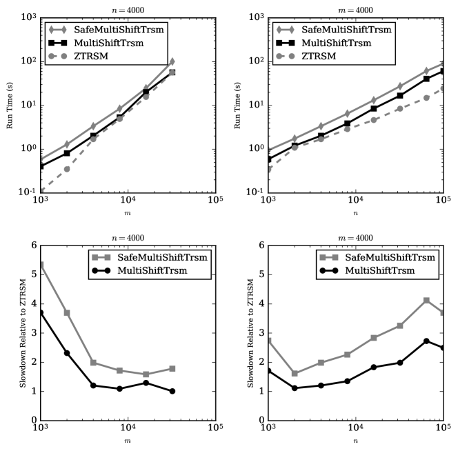
Numerical experiments with the multi-shift triangular solve and safe multi-shift triangular solve were performed with two 4-core Intel Haswell Xeon E5-2623 v3 CPUs at 3.00 GHz. All calculations were performed with double-precision complex numbers and BLAS calls were performed with Intel MKL. A scaling study of the multi-shift triangular solve and safe multi-shift triangular is presented in Figure 1. The safe multi-shift triangular solve was consistently slower than the standard multi-shift triangular solve, which was in turn slower than the Level 3 BLAS triangular solve routine ZTRSM. The performance of the multi-shift triangular solve and safe multi-shift triangular solve were especially poor when the number of right-hand sides was much larger than the matrix dimension, i.e. $m\ll n$. However, when $m\geq n$, we see that the performance of the multi-shift triangular solve is typically within a factor of 1.5 of Level 3 BLAS performance and that the safe multi-shift triangular solve is typically within a factor of 2.

Figure 1: Scaling study of triangular solve, multi-shift triangular solve, and safe multi-shift triangular solve. Matrices were generated by finding Hermitian matrices with uniform random eigenvalues in the interval $\left[1,2\right]$ and deleting entries in the strict lower triangle. Shifts were drawn uniform randomly from the ball $B\left(1.5,0.5\right)$.

7.2 Eigenvector Computation

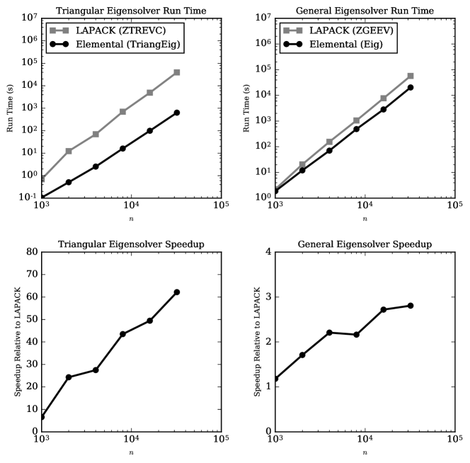
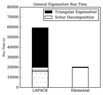
Timing experiments with the triangular and general eigensolvers were performed with the same setup as above (two 4-core Intel Haswell Xeon E5-2623 v3 CPUs at 3.00 GHz, double-precision complex data type, Intel MKL). Scaling studies of the triangular eigensolver and general eigensolver are shown in Figure 2. The triangular eigensolver appears to be asymptotically faster than the LAPACK routine ZTREVC and we report a speedup by a factor of 60 on a $32000\times 32000$ matrix. The general eigensolver appears to converge to a threefold speedup relative to the LAPACK routine ZGEEV. If we inspect the time spent in each stage of the calculation, as shown in Figure 3, we see that Elemental and LAPACK take nearly the same amount of time to compute a Schur decomposition. However, roughly two thirds of LAPACK’s run time takes place in the triangular eigensolver while Elemental’s triangular eigensolver takes a negligible amount of time.

Figure 2: Timing experiments for triangular and general eigensolvers. Matrices were generated by choosing entries uniform randomly from the unit ball.

Figure 3: Timings for the general eigensolvers in LAPACK (ZGEEV) and Elemental (Eig). A $32000\times 32000$ matrix was generated by choosing entries uniform randomly from the unit ball. The timing for LAPACK’s Schur decomposition is subdivided into three stages: ZGEHRD (dots), ZUNGHR (stripes), ZHSEQR (no pattern). The timing for Elemental’s triangular eigensolver includes back transformation.

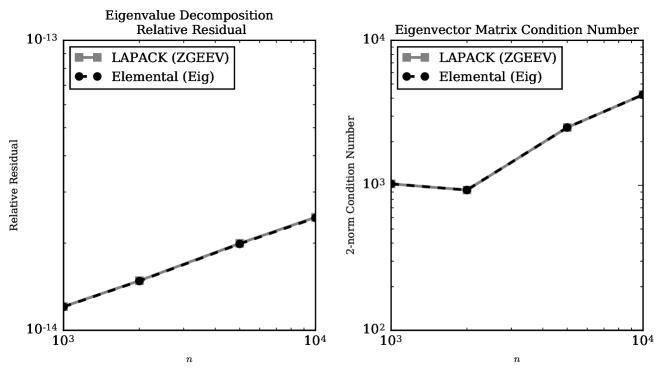
The eigenvalue decomposition $A=X\Lambda X^{-1}$ can be validated by computing the relative residual ${{\left\lVert AX-X\Lambda\right\rVert}_{F}}/{{\left\lVert A\right\rVert}_{F}}$ and the 2-norm condition number $\left\lVert X\right\rVert_{2}\left\lVert X^{-1}\right\rVert_{2}$. As shown in Figure 4, Elemental yields nearly identical results to LAPACK. In particular, the relative residuals are smaller than $10^{-13}$ and the condition numbers are not singular, suggesting that both eigensolvers achieve reasonable quality.

Figure 4: Scaling study for triangular and general eigensolvers. Matrices were generated by choosing entries uniform randomly from the unit ball.

7.3 Pseudospectra Computation

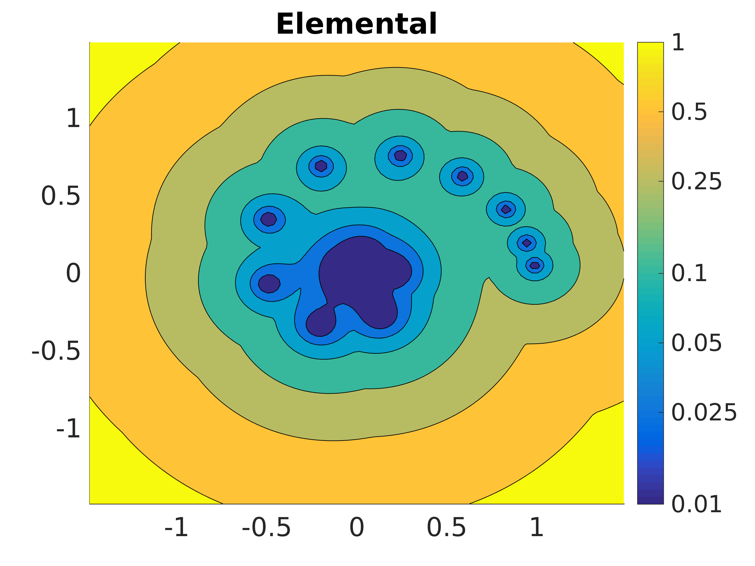
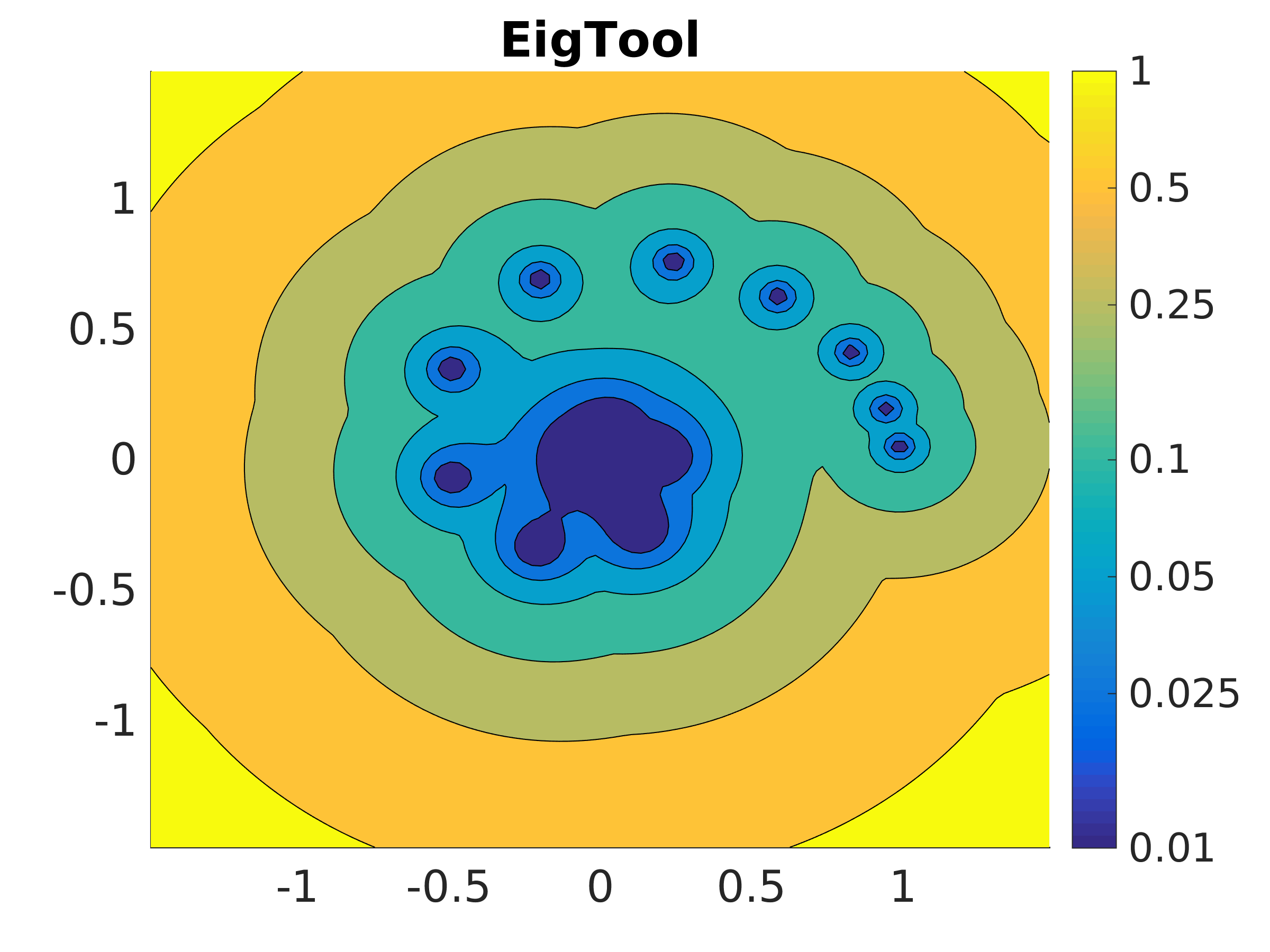
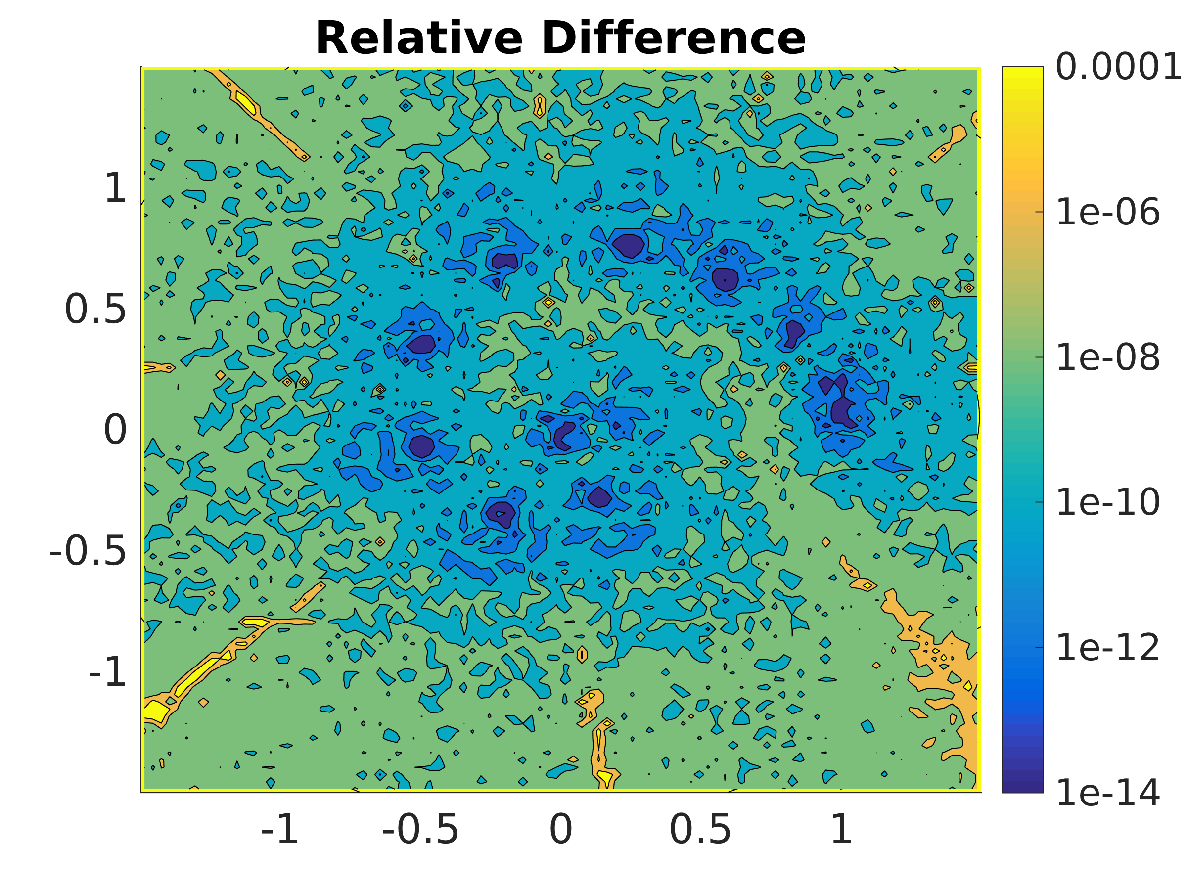
Experiments with pseudospectra solvers were performed with a 4-core Intel Nehalem Core i7-870 CPU at 2.93 GHz. Calculations were performed with double-precision complex numbers and BLAS calls were performed with Intel MKL (for both Elemental and MATLAB). Pseudospectra computed by Elemental and EigTool are qualitatively identical, as shown in Figure 5.

(a)	(b)	(c)

Figure 5: $\epsilon$-pseudospectra with several values of $\epsilon$ and the relative difference in computed resolvent norm. The matrix is a $100\times 100$ discretization of the Fox/Li operator with parameter $F=10$ and the image is constructed from the resolvent norm computed at 10000 grid points [11]. See Chapter 60 of [20] for a discussion on the pseudospectra of the Fox/Li operator.

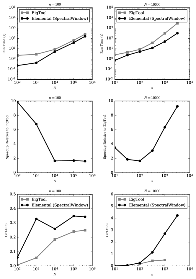
Scaling studies of pseudospectra computation are shown in Figure 6. Given sufficiently many grid points, we see that Elemental achieves a speedup by a factor of 1.6 when computing pseudospectra of a $100\times 100$ matrix. This modest result can be explained by noting that Krylov eigensolvers like the Lanczos method or Arnoldi method require tridiagonal or Hessenberg eigensolvers. When the matrix dimension is small, these eigensolvers take a non-trivial portion of the computation. However, when the matrix dimension is large, the computation is dominated by triangular solves. In this regime, Elemental’s pseudospectra solver fully exploits Level 3 BLAS performance and achieves a ninefold speedup when computing the resolvent norm of a $3200\times 3200$ matrix at $10000$ grid points.

Figure 6: Scaling study for pseudospectra computation on discretizations of the Fox/Li operator with parameter $F=10$ [11].

8 Conclusion

We have shown that multi-shift triangular solves can be performed efficiently by exploiting Level 3 BLAS routines. Numerical experiments suggest that using a safe multi-shift triangular solve to compute triangular eigenvectors is substantially faster than the algorithm presently used in LAPACK, yielding a 60x speedup when computing the eigenvectors of a triangular matrix and a 3x speedup for a general matrix. Pseudospectra computation with multi-shift triangular solves also appears to exhibit a ninefold speedup relative to EigTool when the matrix dimension is sufficiently large. Future work will include real arithmetic multi-shift triangular solves and Fortran implementations for inclusion into LAPACK.

9 Acknowledgments

Tim Moon was supported by a Simons Graduate Research Assistantship and Jack Poulson by AFRL Contract FA8750-12-2-0306.

Appendix A Generalized Multi-Shift Triangular Solve

The multi-shift triangular solve problem can be generalized and applied to compute generalized eigenvectors. Given $m\times m$ upper triangular matrices $U$ and $V$, right-hand side vectors $b_{1},\cdots,b_{n}$, and shifts $\lambda_{1},\cdots,\lambda_{n}$, we seek solution vectors $x_{1},\cdots,x_{n}$ such that

$$\left(U-\lambda_{j}V\right)x_{j} =b_{j}.$$ (16)

This problem can be solved with small modifications to Algorithm 3:

Algorithm 8 Generalized multi-shift triangular solve with blocked back substitution

procedure GeneralizedMultiShiftTrsm($U,V,\lambda,B$) $\triangleright$ $B$ is overwritten with $X$

     for $i=m-n_{b}+1:-n_{b}:1$ do $\triangleright$ Assume $m$ is a multiple of $n_{b}$

         $\mathcal{I}_{0}:=1:i-1$

         $\mathcal{I}_{1}:=i:i+n_{b}-1$

         for $j=1:n$ do

              $U^{\prime}:=U(\mathcal{I}_{1},\mathcal{I}_{1})-\lambda(j)*V(\mathcal{I}_{1},\mathcal{I}_{1})$ $\triangleright$ xAXPY

              Trsv($U^{\prime},B(\mathcal{I}_{1},j)$) $\triangleright$ xTRSV

              $C(:,j):=\lambda(j)*B(\mathcal{I}_{1},j)$ $\triangleright$ xSCAL          

         $B(\mathcal{I}_{0},:):=B(\mathcal{I}_{0},:)-U(\mathcal{I}_{0},\mathcal{I}_{1})*B(\mathcal{I}_{1},:)$ $\triangleright$ xGEMM

         $B(\mathcal{I}_{0},:):=B(\mathcal{I}_{0},:)+V(\mathcal{I}_{0},\mathcal{I}_{1})*C$ $\triangleright$ xGEMM      

Making similar changes to Algorithm 5 yields a robust algorithm:

Algorithm 9 Safe, generalized multi-shift triangular solve with safeguarded, blocked back substitution

procedure SafeGeneralizedMultiShiftTrsm($U,V,\lambda,B,s$) $\triangleright$ $B$ is overwritten with $X$

     $s:=\left[1,\cdots,1\right]^{T}$ $\triangleright$ $n$ entries

     for $j=1:n$ do

         $G(j):=\left\lVert B(:,j)\right\rVert_{\infty}$      

     for $i=m-n_{b}+1:-n_{b}:1$ do $\triangleright$ Assume $m$ is a multiple of $n_{b}$

         $\mathcal{I}_{0}:=1:i-1$

         $\mathcal{I}_{1}:=i:i+n_{b}-1$

         $\mathcal{I}_{2}:=i+n_{b}:m$

         for $j=1:n$ do

              $U^{\prime}:=U(\mathcal{I}_{1},\mathcal{I}_{1})-\lambda(j)*V(\mathcal{I}_{1},\mathcal{I}_{1})$ $\triangleright$ xAXPY

              SafeTrsv($U^{\prime},B(\mathcal{I}_{1},j),t$) $\triangleright$ Diagonal block step

              if $t<1$ then

                  $B(\mathcal{I}_{0},j):=t*B(\mathcal{I}_{0},j)$ $\triangleright$ xSCAL

                  $B(\mathcal{I}_{2},j):=t*B(\mathcal{I}_{2},j)$ $\triangleright$ xSCAL

                  $s(j):=t*s(j)$

                  $G(j):=t*G(j)$               

              $C(:,j):=\lambda(j)*B(\mathcal{I}_{1},j)$ $\triangleright$ xSCAL          

         for $j=1:n$ do

              $G(j):=G(j)+\sum_{k\in\mathcal{I}_{1}}\left(\left\lVert U(\mathcal{I}_{0},k)\right\rVert_{\infty}+\left|\lambda(j)\right|{\left\lVert V(\mathcal{I}_{0},k)\right\rVert}_{\infty}\right)\left\lVert B(\mathcal{I}_{1},j)\right\rVert_{\infty}$

              if $G(j)\geq\Omega$ then

                  Choose $t\in\left(0,1\right)$ so that $t*G(j)<\Omega$

                  $B(:,j):=t*B(:,j)$ $\triangleright$ xSCAL

                  $s(j):=t*s(j)$

                  $G(j):=t*G(j)$                        

         $B(\mathcal{I}_{0},:):=B(\mathcal{I}_{0},:)-U(\mathcal{I}_{0},\mathcal{I}_{1})*B(\mathcal{I}_{1},:)$ $\triangleright$ xGEMM

         $B(\mathcal{I}_{0},:):=B(\mathcal{I}_{0},:)+V(\mathcal{I}_{0},\mathcal{I}_{1})*C$ $\triangleright$ xGEMM      

This routine can be used to solve the generalized eigenvalue problem:

Algorithm 10 Generalized, triangular and generalized, general eigensolvers

function GeneralizedTriangEig($T,S$)

     $\lambda:=\text{diag}(T)./\text{diag}(S)$

     $Z:=-T+S*\text{diag}(\lambda)$

     $\text{diag}(Z):=0$

     $s:=\left[1,\cdots,1\right]^{T}$

     SafeGeneralizedMultiShiftTrsm($T,S,\lambda,Z,s$)

     $\text{diag}(Z):=s$

     return $\lambda,Z$

function GeneralizedEig($A$)

     Compute generalized Schur decomposition $A=QTP^{H},B=QSP^{H}$

     $\lambda,Z:=$ GeneralizedTriangEig($T,S$)

     $X:=PZ$ $\triangleright$ xGEMM

     return $\lambda,X$

References

- [1] E Anderson, Z Bai, C Bischof, S Blackford, J Demmel, J Dongarra, J Du Croz, A Greenbaum, S Hammarling, A McKenney, and D Sorensen. LAPACK Users’ Guide. Society for Industrial and Applied Mathematics, Philadelphia, PA, third edition, 1999.
- [2] Edward Anderson. Robust triangular solves for use in condition estimation. University of Tennessee. Computer Science Department, 1991.
- [3] Z Bai, James Demmel, and A McKenney. On the conditioning of the nonsymmetric eigenproblem: Theory and software. 1989.
- [4] Christian H Bischof, Biswa Nath Datta, and Avijit Purkayastha. A parallel algorithm for the Sylvester observer equation. SIAM Journal on Scientific Computing, 17(3):686–698, 1996.
- [5] Karen Braman, Ralph Byers, and Roy Mathias. The multishift QR algorithm. part I: Maintaining well-focused shifts and level 3 performance. SIAM Journal on Matrix Analysis and Applications, 23(4):929–947, 2002.
- [6] Karen Braman, Ralph Byers, and Roy Mathias. The multishift QR algorithm. part II: Aggressive early deflation. SIAM Journal on Matrix Analysis and Applications, 23(4):948–973, 2002.
- [7] Jack J Dongarra, Jermey Du Cruz, Sven Hammerling, and Iain S Duff. Algorithm 679: A set of level 3 basic linear algebra subprograms: model implementation and test programs. ACM Transactions on Mathematical Software, 16(1):18–28, 1990.
- [8] Jack J Dongarra, Jeremy Du Croz, Sven Hammarling, and Iain S Duff. A set of level 3 basic linear algebra subprograms. ACM Transactions on Mathematical Software, 16(1):1–17, 1990.
- [9] Jack J Dongarra, Jeremy Du Croz, Sven Hammarling, and Richard J Hanson. Algorithm 656: an extended set of basic linear algebra subprograms: model implementation and test programs. ACM Transactions on Mathematical Software, 14(1):18–32, 1988.
- [10] Jack J Dongarra, Jeremy Du Croz, Sven Hammarling, and Richard J Hanson. An extended set of Fortran basic linear algebra subroutines. ACM Transactions on Mathematical Software, 14(1):1–17, 1988.
- [11] Arthur G Fox and Tingye Li. Resonant modes in a maser interferometer. Bell System Technical Journal, 40(2):453–488, 1961.
- [12] Mark Gates, Azzam Haidar, and Jack Dongarra. Accelerating computation of eigenvectors in the dense nonsymmetric eigenvalue problem. In High Performance Computing for Computational Science–VECPAR 2014, pages 182–191. Springer, 2014.
- [13] Gene H Golub and Charles F Van Loan. Matrix Computations. The John Hopkins University Press, 4 edition, 2013.
- [14] Greg Henry. The shifted Hessenberg system solve computation. Citeseer, 1994.
- [15] Nicholas J Higham and Françoise Tisseur. A block algorithm for matrix 1-norm estimation, with an application to 1-norm pseudospectra. SIAM Journal on Matrix Analysis and Applications, 21(4):1185–1201, 2000.
- [16] Chuck L Lawson, Richard J. Hanson, David R Kincaid, and Fred T. Krogh. Basic linear algebra subprograms for Fortran usage. ACM Transactions on Mathematical Software, 5(3):308–323, 1979.
- [17] SH Lui. Computation of pseudospectra by continuation. SIAM Journal on Scientific Computing, 18(2):565–573, 1997.
- [18] Jack Poulson, Bryan Marker, Robert A Van de Geijn, Jeff R Hammond, and Nichols A Romero. Elemental: A new framework for distributed memory dense matrix computations. ACM Transactions on Mathematical Software, 39(2):13, 2013.
- [19] Gregorio Quintana-Ortí and Robert van de Geijn. Improving the performance of reduction to Hessenberg form. ACM Transactions on Mathematical Software, 32(2):180–194, 2006.
- [20] Lloyd Nicholas Trefethen and Mark Embree. Spectra and Pseudospectra: The Behavior of Nonnormal Matrices and Operators. Princeton University Press, 2005.
- [21] Charles Van Loan. How near is a stable matrix to an unstable matrix? Technical report, Cornell University, 1984.
- [22] Field G Van Zee and Robert A Van De Geijn. BLIS: A framework for rapidly instantiating BLAS functionality. ACM Transactions on Mathematical Software, 41(3):14, 2015.
- [23] Qian Wang, Xianyi Zhang, Yunquan Zhang, and Qing Yi. AUGEM: automatically generate high performance dense linear algebra kernels on x86 CPUs. In Proceedings of the International Conference on High Performance Computing, Networking, Storage and Analysis, page 25. ACM, 2013.
- [24] R Clint Whaley and Antoine Petitet. Minimizing development and maintenance costs in supporting persistently optimized BLAS. Software: Practice and Experience, 35(2):101–121, 2005.
- [25] Thomas G Wright. EigTool. http://www.comlab.ox.ac.uk/pseudospectra/eigtool/, 2002.
- [26] Xianyi Zhang, Qian Wang, and Yunquan Zhang. Model-driven level 3 BLAS performance optimization on Loongson 3A processor. In 2012 IEEE 18th International Conference on Parallel and Distributed Systems, pages 684–691. IEEE, 2012.