An intrinsic hyperboloid approach for
Einstein Klein-Gordon equations

Abstract.

In [7] Klainerman introduced the hyperboloidal method to prove the global existence results for nonlinear Klein-Gordon equations by using commuting vector fields. In this paper, we extend the hyperboloidal method from Minkowski space to Lorentzian spacetimes. This approach is developed in [14] for proving, under the maximal foliation gauge, the global nonlinear stability of Minkowski space for Einstein equations with massive scalar fields, which states that, the sufficiently small data in a compact domain, surrounded by a Schwarzschild metric, leads to a unique, globally hyperbolic, smooth and geodesically complete solution to the Einstein Klein-Gordon system.

In this paper, we set up the geometric framework of the intrinsic hyperboloid approach in the curved spacetime. By performing a thorough geometric comparison between the radial normal vector field induced by the intrinsic hyperboloids and the canonical $\partial_{r}$, we manage to control the hyperboloids when they are close to their asymptote, which is a light cone in the Schwarzschild zone. By using such geometric information, we not only obtain the crucial boundary information for running the energy method in [14], but also prove that the intrinsic geometric quantities including the Hawking mass all converge to their Schwarzschild values when approaching the asymptote.

1. Introduction

We introduce the intrinsic hyperboloid approach in the dynamic, Lorentzian spacetime. This approach is developed in [14] to prove, under the maximal foliation gauge, the global stability of Minkowski space for Einstein equations with massive scalar fields, which reads as

$${\emph{\bf{R}}}_{\mu\nu}-\frac{1}{2}\mathbf{g}_{\mu\nu}{\emph{\bf{R}}}=\mathcal{T}_{\mu\nu}$$

with the stress-energy tensor

$$\mathcal{T}_{\mu\nu}=\partial_{\mu}\phi\partial_{\nu}\phi-{\frac{1}{2}}\mathbf{g}_{\mu\nu}\left(\mathbf{g}^{\alpha\beta}\partial_{\alpha}\phi\partial_{\beta}\phi+\mathfrak{m}^{2}\phi^{2}\right),\quad\quad\mathfrak{m}=1,$$

where ${\emph{\bf{R}}}_{\mu\nu}$ and R denote the Ricci curvature tensor and the scalar curvature of the Lorenzian metric $\mathbf{g}$ respectively. Applying the conservation law ${\emph{\bf{D}}}^{\mu}\mathcal{T}_{\mu\nu}=0$, which is due to the Bianchi identity, gives the Einstein Klein-Gordon system

$${\emph{\bf{R}}}_{\alpha\beta} =\partial_{\alpha}\phi\cdot\partial_{\beta}\phi+{\frac{1}{2}}\,\mathbf{g}_{\alpha\beta}\phi^{2},$$ (1.1)

$$\Box_{\mathbf{g}}\phi =\mathfrak{m}^{2}\phi.$$ (1.2)

It is obvious that $({\mathbb{R}}^{3+1},{\bf m},\phi\equiv 0)$, with ${\bf m}$ being Minkowski, trivially solves the system. To construct nontrivial global solutions of (1.1)-(1.2), it is natural to consider the Cauchy problems with the initial data set being small perturbations of the trivial one.

We first briefly review the framework for studying the Cauchy problem of the Einstein equations. Let $(\mathbf{M},\mathbf{g})$ be globally hyperbolic which means that there is a Cauchy hypersurface, which is a spacelike hypersurface with the property that any causal curve intersects it at precisely one point. This allows $\mathbf{M}$ to be foliated by the level surfaces $\Sigma_{t}$ of a time function $t$. Let T be the future directed unit normal to $\Sigma_{t}$. Let $\boldsymbol{\pi}$ be the second fundamental form of $\Sigma_{t}$ in $\mathbf{M}$ defined by

$$\boldsymbol{\pi}(X,Z):=-{\bf g}({\bf D}_{X}{\bf T},Z),\quad X,Z\in\mathcal{T}\Sigma_{t},$$ (1.3)

where ${\bf D}$ denotes the covariant differentiation of $\bf{g}$ in $\mathbf{M}$.

Let $g$ be the induced metric of $\mathbf{g}$ on $\Sigma_{t}$. We decompose

$$\partial_{t}=n{\emph{\bf{T}}}+Y,$$

where $n$ is the lapse function and $Y\in\mathcal{T}\Sigma_{t}$ is the shift vector field. Assuming $Y=0$, then the metric $\mathbf{g}$ can be written as

$$\mathbf{g}=-n^{2}dt^{2}+g_{ij}dx^{i}dx^{j},$$ (1.4)

and the Einstein equations are equivalent to the evolution equations

$$\partial_{t}g_{ij}=-2n{\boldsymbol{\pi}}_{ij},$$ (1.5)

$$\partial_{t}\boldsymbol{\pi}_{ij}=-\nabla_{i}\nabla_{j}n+n(-{\emph{\bf{R}}}_{ij}+R_{ij}+\mbox{Tr}\boldsymbol{\pi}\,\boldsymbol{\pi}_{ij}-2\boldsymbol{\pi}_{ia}\boldsymbol{\pi}^{a}_{j})$$ (1.6)

together with the constraint equations

$$R-|\boldsymbol{\pi}|^{2}+(\mbox{Tr}\boldsymbol{\pi})^{2}=2{\emph{\bf{R}}}_{{\emph{\bf{T}}}{\emph{\bf{T}}}}+{\emph{\bf{R}}},\qquad\nabla^{j}\boldsymbol{\pi}_{ji}-\nabla_{i}\mbox{Tr}\boldsymbol{\pi}={\emph{\bf{R}}}_{{\emph{\bf{T}}}i},$$ (1.7)

where $\mbox{Tr}\boldsymbol{\pi}:=g^{ij}\boldsymbol{\pi}_{ij}$ is the mean curvature of $\Sigma_{t}$ in ${\bf M}$, $\nabla$ denotes the covariant differentiation of $g$, $R_{ij}$ and $R$ are the Ricci curvature and the scalar curvature of $g$ on $\Sigma_{t}$.

The maximal foliation gauge imposes

$$Y=0\quad\mbox{ and }\quad\mbox{Tr}\boldsymbol{\pi}=0\quad\mbox{ on }\Sigma_{t}.$$ (1.8)

This implies $n$ satisfies the elliptic equation

$$\Delta_{g}n-|\boldsymbol{\pi}|^{2}n=n{\emph{\bf{R}}}_{{\emph{\bf{T}}}{\emph{\bf{T}}}}\qquad\mbox{on }\Sigma_{t},$$ (1.9)

and the second fundamental form $\boldsymbol{\pi}$ satisfies the Codazzi equation

$$\mbox{\,div\,}\boldsymbol{\pi}={\emph{\bf{R}}}_{{\emph{\bf{T}}}i},\quad\mbox{\,curl\,}\boldsymbol{\pi}=H,$$ (1.10)

where $H$ is the magnetic part of the Weyl curvature, defined in (4.8).

The first proof of the global stability of Minkowski spacetime for generic, asymptotically flat data is provided in the monumental work [1], where the Einstein vacuum Bianchi equation is thoroughly and systematically treated. Heuristically, we regard the nonlinear wave equation verifying the standard null condition as the vastly simplified model for the Einsteinian Bianchi equation. Then (1.1)-(1.2) is a coupled system between such nonlinear wave equations and the Klein-Gordon equation in the Einsteinian background. Due to the presence of the massive scalar field, the approach we introduce in this paper is to twist the hyperboloidal energy method devised in the flat spacetime in [7] for the Klein-Gordon equations to the Lorentzian spacetime, in the sense of incorporating it to the intrinsic energy scheme devised in [1]. Such generalization triggers fundamental changes to the geometry of the intrinsic framework in [1] for the Einstein equations, which by itself is very challenging even merely for the vacuum case. Our approach is robust for treating both the scalar field and the Einstein part of the equation system. This will be fully confirmed in [14].

In what follows, we will use the linear Klein-Gordon equation to motivate the use of the intrinsic hyperboloids. To begin with, let us recall some basics of the invariant vector fields for the free wave $\Box_{\bf m}\phi=0$. We denote by $Z$ a set of vector fields, which consists of the translation $\partial_{\mu},$ the scaling vector field $S=x^{\mu}\partial_{\mu}$ and the generator of Lorentz group

$$\Omega_{\mu\nu}=x_{\mu}\partial_{\nu}-x_{\nu}\partial_{\mu},\quad\mu,\nu=0,1,2,3\mbox{ where }x_{\mu}={\bf m}_{\mu\nu}x^{\nu}.$$ (1.11)

This set of vector fields is named as commuting vector fields due to the fundamental property

$$[\Box_{\bf m},Z]=0\mbox{ or }2\Box_{\bf m}$$ (1.12)

with the second identity occurring only when $Z=S$.

In order to get the decay estimate $(t+1)|\phi|\lesssim 1$ by the energy approach, we rely on two ingredients: one is the boundedness of the energy or the generalized energy; the other is the Klainerman-Sobolev inequality.

The standard Klainerman-Sobolev inequality

$$\langle t\rangle(1+|t-r|)^{\frac{1}{2}}|f|\lesssim\|Z^{(\leq 2)}f(t,\cdot)\|_{L^{2}({\mathbb{R}}^{3})}$$ (1.13)

relies on the full set of $Z$ derivatives, where $r=(\sum_{i=1}^{3}|x^{i}|^{2})^{1/2}$, $\langle t\rangle=t+1$ and $Z^{(\leq m)}f$ denotes the application of the differential operators in $Z$ to $f$ up to $m$ times. For the free wave equation $\Box_{\bf m}\phi=0$, by using $\partial_{t}$ as a multiplier, one can obtain the conserved energy

$$\|\partial_{t}\phi(t,\cdot)\|^{2}_{L^{2}({\mathbb{R}}^{3})}+\sum_{i=1}^{3}\|\partial_{x^{i}}\phi(t,\cdot)\|^{2}_{L^{2}({\mathbb{R}}^{3})}.$$ (1.14)

By using the canonical Morawetz vector field, $K=2tS-(t^{2}-r^{2})\partial_{t},$ as a multiplier, one can obtain the conserved generalized energy, which is uniformly comparable for $t\geq 0$ to

$$\|Z\phi(t,\cdot)\|^{2}_{L^{2}({\mathbb{R}}^{3})}+\|\phi(t,\cdot)\|^{2}_{L^{2}({\mathbb{R}}^{3})}.$$ (1.15)

In view of (1.12), one can see that (1.14) and (1.15) hold with $\phi$ replaced by $Z^{\!(n)}\phi$. These estimates together with (1.13) imply that

$$\langle t\rangle(1+|t-r|)^{\frac{1}{2}}|\phi|\lesssim\|Z^{\!(\leq 2)}\phi(0,\cdot)\|_{L^{2}({\mathbb{R}}^{3})}\lesssim 1$$ (1.16)

which gives more information for $\phi$ than desired.

To see the difference in the treatment for the Klein-Gordon equation, we consider the linear Klein-Gordon equation

$$\Box_{\bf m}\phi=\phi$$ (1.17)

in the Minkowski spacetime. Due to (1.12) there holds $[(\Box_{\bf m}-1),S]=2\Box_{{\bf m}}\neq 2(\Box_{{\bf m}}-1)$. Thus the scaling vector field $S$ can not be used as a commuting vector field for (1.17). Similar to (1.14), we can obtain the conserved energy

$$\|\partial_{t}\phi(t,\cdot)\|^{2}_{L^{2}({\mathbb{R}}^{3})}+\sum_{i=1}^{3}\|\partial_{x^{i}}\phi(t,\cdot)\|^{2}_{L^{2}({\mathbb{R}}^{3})}+\|\phi(t,\cdot)\|^{2}_{L^{2}({\mathbb{R}}^{3})}$$

which stays conserved if $\phi$ is replaced by $Z^{\!(n)}\phi$ except $Z=S$. In contrast to the case of the free wave, the boundedness of energy does not hold for the full set of the commuting vector fields in $Z$. The Klainerman-Sobolev inequality (1.13) can not be used directly. To get the decay estimates for the Klein-Gordon equations, in [7] the Klainerman-Sobolev inequality is applied on the canonical hyperboloids ${\mathbb{H}}_{\rho}=\{t^{2}-\sum_{i=1}^{3}|x^{i}|^{2}=\rho^{2}\}$ which are the surfaces orthogonal to $S$. The Klainerman-Sobolev inequality on hyperboloids merely relies on the Lorentz boosts $\{R_{i}=t\partial_{x^{i}}+x^{i}\partial_{t},i=1,2,3\}$ which are commuting vector fields of (1.17) and tangent to the hyperboloids. By virtue of this tool, the standard sharp decay estimate

$$\langle t\rangle^{\frac{3}{2}}|\phi|\lesssim\left\|\left(\frac{t}{\rho}\right)^{\frac{1}{2}}R^{(\leq 2)}\phi(\rho,\cdot)\right\|_{L^{2}(\mathbb{H}_{\rho})}\lesssim\left\|\partial^{\!(\leq 1)}R^{(\leq 2)}\phi(0,\cdot)\right\|_{L^{2}(\mathbb{R}^{3})}.$$ (1.18)

can be derived from the boundedness of energies on hyperboloids. Thus, in order to get the sharp decay for the solutions of (1.17), the same order of commuting vector fields are applied and energies have to be controlled up to one order higher compared with the free wave case. This coincides with the case when we treat Klein-Gordon equation (1.2) coupled with the Einstein Bianchi equations, for which (1.17) and the free wave are the simplest toy models for each part.

We also observe that the two weighted multipliers, $S$ and $K$, can not be used to obtain bounded generalized energy for (1.17). This fact together with the fact that the scaling $S$ is not a commuting vector field for (1.17), demonstrates that decomposing $\partial\phi$ in terms of the null frame $\{L=\partial_{t}+\partial_{r},{\underline{L}}=\partial_{t}-\partial_{r}\}$ does not improve the decay along the good direction $L$. This is another difference compared with the free wave. Contributed by the commuting vector fields $R$, $\partial\phi$ exhibits much stronger decay along the tangential directions of ${\mathbb{H}}_{\rho}$; however, $\partial\phi$ has the weakest decay along $B:=\frac{t}{\rho}\partial_{t}+\frac{r}{\rho}\partial_{r}=\rho^{-1}S$, the future directed unit normal of ${\mathbb{H}}_{\rho}$. The weakest decay is much weaker than that a free wave exhibits along its only bad direction ${\underline{L}}$.

Figure 1(a) depicts the method in [7], where the data with compact support in $\{r\leq R\}$ are given at $t=0$. The energy argument is divided into two steps. The first step is the local energy propagation from $t=0$ to the initial hyperboloidal slice ${\mathbb{H}}_{\rho_{0}}$, with $\rho_{0}\approx 1$. The second step is to propagate energy on hyperboloids ${\mathbb{H}}_{\rho}$ from ${\mathbb{H}}_{\rho_{0}}$ to the last slice ${\mathbb{H}}_{\rho_{*}}$, in the region enclosed by a Minkowskian light cone as the boundary, along which the solution varnishes due to finite speed of propagation. This figure gives us the blue-print of treating the Einstein-Klein-Gordon system.

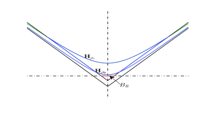
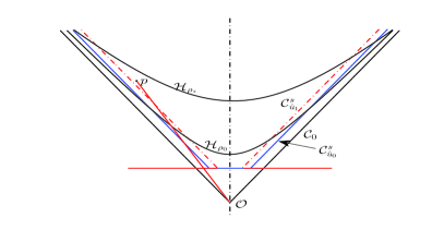
Figure 1.

In order to set up the Cauchy problem for the Einstein-Klein-Gordon system (1.1)-(1.2) appropriately, to match with, in particular, the scenario that the data for Klein-Gordon equation have compact support, we consider the initial data set $(g_{0},\boldsymbol{\pi}_{0},\phi[0])$ for (1.1)-(1.2), which verify the Einstein constraint equations (1.7) and $\phi[0]$ is compactly supported within $B_{1}$, the unit Euclidian ball. Outside of the co-centered Euclidean ball of radius $2$, there glues a surrounding Schwarzschild metric specified at Theorem 4.6. See Figure 1(b). We will call the region with $t\geq 0$, exterior to the Schwarzschild outgoing light cone ${\mathcal{C}}^{s}_{\hat{u}_{1}}$ as the Schwarzschild zone $Z^{s}$, where ${\mathcal{C}}^{s}_{\hat{u}_{1}}$ initiates from the Euclidean sphere $\{r=2\}$ with the value of $\hat{u}_{1}$ specified in Section 4.4. We still need to determine the foliation of hyperboloids in the curved spacetime.

There are two options at this point. One way is based entirely on the symmetry and geometry in Minkowski space. This method has been developed in [8] and [9] for the Einstein equations under the wave coordinates. The philosophy of the regime is to close the energy argument without aiming at achieving sharp decay for geometric quantities. This allows the stability result to be achieved within a much smaller framework compared with [1]. However it is less precise on the asymptotic behavior of the solution (see [8, Page 47]).

In this paper and [14], we take the other option which constructs intrinsic hyperboloids adapted to the curved spacetimes. We not only prove the global nonlinear stability, but also give a comprehensive, analytic, global-in-time depiction of the solution. The goal of this paper is to introduce the geometric framework, which equips the nonlinear analysis with sets of tetrads, recovering the symmetry and playing the role of coordinates, all of which are adapted to the dynamical spacetime. The global existence of such tetrads will be justified simultaneously with the quantitative depiction of the spacetime.

When setting up the geometric framework, it is necessary to discriminate, among all the symmetry in the Minkowski space, the most crucial geometric information that needs precision from those allowing error to be controlled analytically. For this purpose, we run a simple energy argument for

$$\Box_{\mathbf{g}}\phi=\phi$$ (1.19)

by taking the approach as in [8], that is to consider

$$\Box_{\mathbf{g}}R^{\!(n)}\phi=R^{\!(n)}\phi+[\Box_{\mathbf{g}},R^{\!(n)}]\phi.$$ (1.20)

The error integral contributed by one term contained in the commutator on the right hand side of (1.20) takes the form

$$\int^{\rho}_{1}\int_{{\mathbb{H}}_{\rho^{\prime}}}{}^{(R)}\pi^{\alpha\beta}\underbrace{R^{(n-1)}{\emph{\bf{D}}}^{2}_{\alpha\beta}\phi}_{\in L^{2}}\cdot\underbrace{{\emph{\bf{D}}}_{\emph{\bf{T}}}R^{(n)}\phi}_{\in L^{2}}d\mu_{{\mathbb{H}}_{\rho^{\prime}}}d\rho^{\prime},$$

where the deformation tensor is defined by

$${}^{(X)}\pi_{\alpha\beta}={\emph{\bf{D}}}_{\alpha}X_{\beta}+{\emph{\bf{D}}}_{\beta}X_{\alpha}$$ (1.21)

with D denoting the connection induced by the metric $\mathbf{g}$. Here $X=R$ is the Lorentz boost in Minkowski space, ${}^{(R)}\pi^{\alpha\beta}\neq 0$ since $\mathbf{g}$ is not the Minkowski metric. With $\alpha,\beta=B$ in ${}^{(R)}\pi^{\alpha\beta}$, the derivative of $\phi$ contracted with this term is evaluated at the bad direction $B$ along which it does not decay strongly. Under local coordinates the expression of ${}^{(R)}\pi^{BB}$ contains $B$ derivatives of the metric $\mathbf{g}$, paired with large weights. The best decay for ${}^{(R)}\pi^{BB}$ expected by the approach from [8] is below the borderline $C{\epsilon}/\rho$ for applying Gronwall inequality to control energies. To salvage the energy argument, we construct a set of approximate Lorentz boosts $\mathscr{R}$ and the intrinsic hyperboloids ${\mathcal{H}}_{\rho}$, adapted to the Einstein background, so that ${}^{(\mathscr{R})}\pi^{\mathfrak{B}\mathfrak{B}}=0$, where $\mathfrak{B}$ denotes the unit normal of the constructed foliation of hyperboloids. These $\mathscr{R}$ and $\mathfrak{B}$ can be viewed as the corresponding replacements of $R$ and $B$ in the curved spacetime. The construction of these $\mathscr{R}$ and $\mathfrak{B}$ needs to preserve the following features:

1. $[\mathfrak{B},\mathscr{R}]=0$ and $\mathscr{R}=\{\mathscr{R}_{i},i=1,2,3\}$ are tangent to ${\mathcal{H}}_{\rho}$.

2. $\cup_{\rho=0}^{\infty}{\mathcal{H}}_{\rho}$ exhausts the chronological future of an origin $\mathcal{O}$, with the origin to be appropriately chosen. All the hyperboloids are asymptotic to the outgoing light cone ${\mathcal{C}}_{0}$ emanating from $\mathcal{O}$.

The origin $\mathcal{O}$ is chosen at $t=-T$, which can be done due to the local extension of the solution. We may choose $T$ so that ${\mathcal{C}}_{0}$ intersects $\{t=0\}$ outside of $B_{4}$. The freedom of such choice is fixed in Section 2, which is crucial for the proof of the main results of this paper. We leave the details of the constructions to Section 2-3. See Proposition 2.3 for using the first feature to prove ${}^{(\mathscr{R})}\pi_{\mathfrak{B}\mathfrak{B}}=0$ and more results on ${}^{(\mathscr{R})}\pi$.

The geometric constructions equip us with the approximate Lorentz boost, scaling, and translation vector fields. With them we can run the commuting vector field approach to the Einstein Bianchi equations, which can be viewed as an extension of the approach in [1], where the regime is based on the construction of the rotation vector fields and the intrinsic null cones. The task, in our situation, is much more involved, due to the difficulties caused by the massive scalar field, the geometry of the hyperboloids, as well as the complexity of the analytic control on the Lorentz boosts. In what follows we focus on addressing the following two basic issues.

1. For the Weyl part of curvature, we will run the regime of Bel-Robinson energies defined by the weighted multipliers $S$ and $K$. For closing the top order energy, we encounter the issue of requiring higher order $\mathscr{R}$-energy for the massive scalar field. However, in order to close the energy estimates, we have to control the energies of the Weyl tensors and the massive scalar field, up to the same order in terms of the $\mathscr{R}$-derivatives.

2. The intrinsic hyperboloids, in principle, are defined from the Minkowskian counterparts by a global diffeomorphism, which needs to be justified simultaneously with the proof of the global existence of the solution. In Minkowski space, the density of the foliation of the canonical hyperboloids approaches infinity near the causal boundary. The control on the intrinsic foliation is considerably more delicate since, analytically, terms of $1/\rho$ type appear frequently, with $\rho\rightarrow 0$ when approaching the causal boundary ${\mathcal{C}}_{0}$.

To solve the first issue, it is crucial to use the Einstein Bianchi equations, see Lemma 4.1, which allows us to perform the integration by parts when treating the worst type of terms. We then take advantage of the null forms in the Einstein Bianchi equations, together with the expected strong decay from the scalar field. This enables the top order energies to be closed at a sharp level. We will sketch briefly the energy scheme in Section 4.

The second issue is connected to the set-up of the wave zone, the region where we run the energy estimates. We have to take account of the gravitational influence to the causal structure of the foliation of the intrinsic hyperboloids. In this paper, we focus on controlling the intrinsic geometry of the chronological future ${\mathcal{I}}^{+}(\mathcal{O})$ for $t\lesssim 1$ and for all $t$ in the Schwarzschild zone. This geometric control is significant for dealing with the problem of leakage, for demonstrating that a constructed function is almost optical, and for justifying an excision procedure on the wave zone for the energy scheme. These aspects will be explained in the sequel.

In the Minkowskian set-up (Figure 1(a)), a light cone is used to cut the family of hyperboloids, as the boundary of the wave zone. The cone needs to be uniformly away from the asymptote. The set-up of such boundary in the curved spacetime is more subtle. First of all, this boundary should be chosen in the Schwarzschild region, to guarantee the dynamical part of the solution is contained in its interior. It ought to be a canonical Schwarzschild light cone ${\mathcal{C}}^{s}_{\hat{u}_{0}}$ for the ease of analysing energy flux therein. More importantly, we need a function measuring the “distance” from any point in the entire wave zone to ${\mathcal{C}}_{0}$, which is the asymptote of the hyperboloids. This nonnegative function needs to be bounded uniformly away from zero in the wave zone, for the purpose of running the energy estimates. This task intuitively could be achieved if ${\mathcal{C}}^{s}_{\hat{u}_{0}}$ is spaced away uniformly from ${\mathcal{C}}_{0}$ in terms of a canonical optical function in $Z^{s}$.

In Lorentzian spacetime the light cones are usually characterized by the level sets of an optical function $u$ (see [1]) which is defined as the solution of the eikonal equation

$$\mathbf{g}^{\alpha\beta}\partial_{\alpha}u\partial_{\beta}u=0$$ (1.22)

with prescribed boundary or initial conditions. Then the optical function $u$ naturally measures the distance to the causal boundary. To obtain the information of $u$ would require geometric controls on the foliations of light cones $C_{u}$. However, since such light cones are not involved in our analysis, we do not use the actual optical function. In our framework, ${\mathcal{H}}_{\rho}$ conceptually replaces the role usually played by $C_{u}$. The geometric control on the hyperboloids ${\mathcal{H}}_{\rho}$ lies at the core of our analysis. To achieve the desired analytic feature, we choose $\rho$ to be the proper time to $\mathcal{O}$, where $\rho$ verifies the eikonal equation

$$\mathbf{g}^{\alpha\beta}\partial_{\alpha}\rho\partial_{\beta}\rho=-1,\quad\rho(\mathcal{O})=0.$$

Throughout the chronological future $({\mathcal{I}}^{+}(\mathcal{O}),\mathbf{g})$, we define an alterative function, still denoted by $u$, which does not verify (1.22), yet taking the role of measuring the distance to ${\mathcal{C}}_{0}$. In particular, we can show that this function $u$, vanishing on ${\mathcal{C}}_{0}$, is sufficiently close to the canonical optical function near ${\mathcal{C}}_{0}$ in $Z^{s}$. To show such property, we perform in Section 5 a full analytic comparison between the radial normal of the Schwarzschild frame and the normal vector field on $\Sigma_{t}$, induced by the foliation of the intrinsic hyperboloid $\cup_{\rho}S_{t,\rho}$. The main estimates are established in Theorem 5.12 throughout $Z^{s}\cap\{\rho\leq\rho_{*}\}$, which is the major building block of this paper. These estimates and their higher order counterparts will be used in the main energy scheme in [14].

Next we address the issue of the leakage. Let $p$ be a point inside the wave zone, near the boundary ${\mathcal{C}}^{s}_{\hat{u}_{0}}$. The distance maximizing timelike geodesic connecting $p$ and $\mathcal{O}$ is not entirely contained in the wave zone. See Figure 1(b). This phenomenon can be easily seen in Minkowski space. In Minkowskian case the deformation tensors of the boosts vanish and the deformation tensor of the scaling vector field has a standard value. However, in the dynamical spacetime, deformation tensors ${}^{(\mathscr{R})}\pi$ and ${}^{(S)}\pi$ need to be analyzed, which is done by integrating along the aforementioned time-like geodesics with the help of the structure equations which contain both the curvature components under the hyperboloidal frame and the second fundamental forms; see Section 3.2. Whether the path of the integration is contained in the wave zone determines how to control the integrand. The geometric information outside of the wave zone can not be provided by the energy estimates. Such information is obtained simultaneously with the main estimates in Section 5 by geometric comparisons and bootstrap arguments.

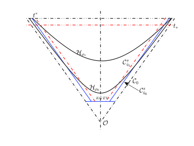
Figure 2. Illustration of wave zone

Now we explain, as part of the energy scheme, the excision of a region which is related to the so-called last slice of hyperboloids, denoted by ${\mathcal{H}}_{\rho_{*}}$. As a standard method for proving global results of non-linear dynamical problem, one can suppose a set of bootstrap assumptions hold till certain maximal life-span. Due to various concerns, we set the maximal life-span in terms of the proper time, labeled by $\rho_{*}$. Once the bootstrap assumptions can be improved for all $\rho\leq\rho_{*}$, by the principle of continuation, the solution and the quantitative control can be extended beyond $\rho_{*}$. The wave zone is a region which is enclosed by the initial slice $\{t=0\}$, the last slice ${\mathcal{H}}_{\rho_{*}}$ as well as the cone ${\mathcal{C}}^{s}_{\hat{u}_{0}}$. Consider the energy estimates on $\Sigma_{t}$, which are crucial for controlling ${}^{({\emph{\bf{T}}})}\pi$. When $t\geq t_{*}$ where $t_{*}:=\min\{t:S_{\rho_{*},\hat{u}_{0}}\}$, we no longer expect a regular subset of $\Sigma_{t}$ within the wave zone to do the energy estimates (see Figure 2 in Section 4). The subset of wave zone with $t\geq t_{*}$ will be excised for obtaining the $\Sigma_{t}$-energy. This may lead to the loss of control of ${}^{({\emph{\bf{T}}})}\pi$ in a region with $t$ large within the wave zone, which would fail the energy control on ${\mathcal{H}}_{\rho}$. Our strategy is to show that the region of excision is fully contained in $Z^{s}$, where ${}^{({\emph{\bf{T}}})}\pi$ and other geometric quantities can be controlled by the main estimates. This proof has to be done merely depending on local energy estimate, and the assumption that the foliation of ${\mathcal{H}}_{\rho}$ exists up to $\rho\leq\rho_{*}$, which is the case in this paper (see Section 6).

As the other application of the main estimates, we show that the Hawking mass is convergent to the ADM mass of the surrounding Schwarzschild metric along every hyperboloid.

Finally, we comment on the analysis of the intrinsic geometry in $Z^{s}$. This analysis is independent of the long-time energy estimates in the wave zone. The idea is to use the transport equations to perform the long-time geometric comparison. We define a set of quantities which encode the deviation between the intrinsic and the extrinsic tetrads, and derive the transport equations for them along well-chosen paths. In order to prove the function $u$ is almost optical, we uncover a series of cancelations, contributed by the Schwarzschild metric and the structure equations of the hyerboloidal foliation. It necessitates delicate bootstrap arguments and weighted estimates. The obtained main estimates are crucial for the applications in Section 6-7.

The paper is organized as follows. In Sections 2-3 we carefully set up the analytic framework of the foliation of intrinsic hyperboloids, and provide the geometric construction of the intrinsic frame of the Lorentz boosts, since such set-up and construction have never appeared in the literature. In Section 4 we sketch the energy scheme in the proof of global stability of Minkowski space for (1.1)-(1.2). In Section 5, by assuming the foliation of the intrinsic hyperboloids and the maximal foliation exist till the last slice of hyperboloid, we provide a thorough depiction of the intrinsic geometry in the Schwarzschild zone, presented in Theorem 5.12, as the main estimates of this paper. The region considered there is the most sensitive region for having the geometric control on hyperboloids. The set of main estimates depends merely on local-in-time energy estimates and the smallness of the given data on the initial maximal slice. We then give applications of the main estimates. The one in Section 6 is to control the region of the excision. In Section 7, we give the asymptotic behavior of the Hawking mass along all hyperboloids.

2. Construction of the boost vector fields

By standard energy and iteration argument, we first solve the Cauchy problem of EKG back to the past to certain fixed $t\leq-T$. Let $\mathbf{o}$ be the spacial origin of the given initial slice. We denote by $\Gamma(t)$ the geodesic through $\mathbf{o}$ with velocity $-{\emph{\bf{T}}}$, where T is the future-directed time-like unit normal of the initial slice $\Sigma_{0}$. The geodesic is extended (back-in-time) within the radius of injectivity of $\mathbf{o}$, intersecting $\{t=-T\}$ at $\mathcal{O}$. $T$ is chosen so that the given Cauchy data at the initial slice is fully contained in $\mathscr{J}^{+}(\mathcal{O})\cap\{t=0\}$, where $\mathscr{J}^{+}(\mathcal{O})$ denotes the causal future of $\mathcal{O}$. Hence $T$ depends on the size of the support of Cauchy data, and is comparable to $1$. To be more precise, $T$ is chosen such that ${\mathcal{C}}_{0}$ intersects at $t=0$ outside of $B_{4}$. Now by the shift of $t^{\prime}=t+T$, as well as an abuse of notation, $t=0$ at $\mathcal{O}$ and the initial data is prescribed at $t=T$, according to the time coordinate after the shift.

We use ${\mathcal{I}}^{+}(\mathcal{O})$ to denote the chronological future of $\mathcal{O}$. Let $i_{*}$ be the time-like radius of injectivity of $\mathcal{O}$, which is defined to be the supremum over all the values $s_{0}>0$ for which the exponential map

$$\exp_{\mathcal{O}}:(\rho,V)\to\Upsilon_{V}(\rho),\quad V\in\mathbb{H}_{1}$$ (2.1)

is a global diffeomorphism from $(0,s_{0})\times\mathbb{H}_{1}$ to its image in ${\mathcal{I}}^{+}(\mathcal{O})$, where

$$\mathbb{H}_{1}:=\left\{V=(V^{0},V^{1},V^{2},V^{3}):(V^{0})^{2}-\sum_{i=1}^{3}(V^{i})^{2}=1\right\}$$

is the canonical hyperboloid in ${\mathbb{R}}^{3+1}$ and $\Upsilon_{V}$ is the time-like geodesic with $\Upsilon_{V}(0)=\mathcal{O}$ and $\Upsilon_{V}^{\prime}(0)=V$. We use ${\mathcal{I}}_{*}^{+}(\mathcal{O})$ to denote the part of ${\mathcal{I}}^{+}(\mathcal{O})$ within the time-like radius of injectivity. In [14] we will prove that the time-like radius of injectivity is $+\infty$ simultaneously when we prove the global well-posedness for EKG, provided the Cauchy data is sufficiently small. Thus we will have ${\mathcal{I}}_{*}^{+}(\mathcal{O})={\mathcal{I}}^{+}(\mathcal{O})$ once this result is established.

For a point $p$ in ${\mathcal{I}}^{+}(\mathcal{O})$, we use $\rho$ to denote its geodesic distance to $\mathcal{O}$. Then $\rho$ is a smooth function on ${\mathcal{I}}_{*}^{+}(\mathcal{O})$ satisfying $\langle{\emph{\bf{D}}}\rho,{\emph{\bf{D}}}\rho\rangle=-1$ with $\rho(\mathcal{O})=0$. We introduce the vector field

$$\mathfrak{B}=-{\emph{\bf{D}}}\rho.$$ (2.2)

Then $\mathfrak{B}$ is geodesic, i.e. ${\emph{\bf{D}}}_{\mathfrak{B}}\mathfrak{B}=0$ and $\langle\mathfrak{B},\mathfrak{B}\rangle=-1$. Using this $\mathfrak{B}$ we define the lapse function ${\mathbf{b}}$ by

$$\langle\mathfrak{B},{\emph{\bf{T}}}\rangle=-{\mathbf{b}}^{-1}\frac{t}{\rho}$$ (2.3)

Let

$${\mathcal{H}}_{\rho}:=\exp_{\mathcal{O}}(\rho{\mathbb{H}}_{1}).$$

Clearly $\{{\mathcal{H}}_{\rho}\}$ are the level sets of $\rho$ which give a foliation of ${\mathcal{I}}_{*}^{+}(\mathcal{O})$ in terms of hyperboloids. Moreover, by the Gauss lemma we can see that $\mathfrak{B}$ is the future directed normal to ${\mathcal{H}}_{\rho}$ and

$$\mathfrak{B}_{p}=\left(d\exp_{\mathcal{O}}\right)_{\rho V}(\partial_{\rho})$$ (2.4)

for any $p\in{\mathcal{I}}_{*}^{+}(\mathcal{O})$, where $(\rho,V)$ is the unique point in $(0,i_{*})\times{\mathbb{H}}_{1}$ such that $p=\exp_{\mathcal{O}}(\rho V)$.

Using $\mathfrak{B}$ we may introduce the second fundament form $k$ of ${\mathcal{H}}_{\rho}$ defined by

$$k(X,Y)=\langle{\emph{\bf{D}}}_{X}\mathfrak{B},Y\rangle$$

where $X,Y$ are vector fields tangent to ${\mathcal{H}}_{\rho}$. Clearly $k$ is an ${\mathcal{H}}_{\rho}$ tangent, symmetric $(0,2)$ tensor. We will use $\mbox{tr}k$ and ${\hat{k}}$ to denote the trace and traceless part of $k$ respectively.

According to the expression of $\mathbf{g}$, we can derive that the future directed unit normal T of $\Sigma_{t}$ takes the form

$${\emph{\bf{T}}}=n^{-1}\partial_{t}.$$ (2.5)

This together with ${\emph{\bf{D}}}t=-n^{-2}\partial_{t}$ and (2.3) implies that

$$\mathfrak{B}(t)=\langle\mathfrak{B},{\emph{\bf{D}}}t\rangle=\frac{{\mathbf{b}}^{-1}n^{-1}t}{\rho}.$$ (2.6)

For future reference, we set

$${t_{\flat}}:=({\mathbf{b}}^{-1}t)(\Gamma(t));\quad{r_{\flat}}=\sqrt{{t_{\flat}}^{2}-\rho^{2}}.$$ (2.7)

According to the definition of ${\mathcal{I}}_{*}^{+}(\mathcal{O})$, for any $p\in{\mathcal{I}}_{*}^{+}(\mathcal{O})$ there corresponds a unique $(\rho,V)\in(0,i_{*})\times{\mathbb{H}}_{1}$ with $V=(V^{0},V^{1},V^{2},V^{3})$ such that

$$p=\exp_{\mathcal{O}}(\rho V).$$ (2.8)

We set

$$y^{0}=\tau:=\rho\sqrt{1+\sum_{i=1}^{3}(V^{i})^{2}}\quad\mbox{and}\quad y^{i}=\rho V^{i}\mbox{ for }i=1,2,3.$$ (2.9)

Then $\{y^{\mu},\mu=0,\cdots 3\}$ gives the geodesic normal coordinates for ${\mathcal{I}}_{*}^{+}(\mathcal{O})$.

Lemma 2.1.

For any $V\in{\mathbb{H}}_{1}$ there hold

$$\lim_{\rho\rightarrow 0}\frac{\tau}{t}(\rho V)=n(\mathcal{O}),\quad\lim_{\rho\rightarrow 0}\frac{{\mathbf{b}}\tau}{t}(\rho V)=1,\quad\lim_{\rho\rightarrow 0}{\mathbf{b}}^{-1}(\rho V)=n(\mathcal{O}).$$ (2.10)

Proof.

By using (2.3) we can consider the local expansion of ${\mathbf{b}}^{-1}t={\frac{1}{2}}{\emph{\bf{D}}}_{\mu}(\rho^{2}){\emph{\bf{T}}}^{\mu}$ at $\mathcal{O}$ as follows

$${\mathbf{b}}^{-1}t =\left.{\mathbf{b}}^{-1}t\right|_{\mathcal{O}}+\left.{\frac{1}{2}}{\emph{\bf{D}}}_{\nu}({\emph{\bf{D}}}_{\mu}(\rho^{2}){\emph{\bf{T}}}^{\mu})\right|_{\mathcal{O}}\rho V^{\nu}+O(\tau^{2})$$

$$=\left.-(\mathbf{g}_{\mu\nu}{\emph{\bf{T}}}^{\mu})\right|_{\mathcal{O}}\rho V^{\nu}-\left.{}^{({\emph{\bf{T}}})}\pi_{\mu\nu}\right|_{\mathcal{O}}\rho^{2}V^{\mu}V^{\nu}+O(\tau^{2})$$

$$=\tau+O(\tau^{2}),$$

where we employed [6, Page 50] to get $\left.{\frac{1}{2}}{\emph{\bf{D}}}_{\nu}{\emph{\bf{D}}}_{\mu}(\rho^{2})\right|_{\mathcal{O}}=-\mathbf{g}_{\mu\nu}(\mathcal{O})$. This implies the second identity in (2.10). Similarly, for the function $n^{-1}t={\frac{1}{2}}{\emph{\bf{T}}}(t^{2})$ we have the local expansion

$$n^{-1}t =\left.{\frac{1}{2}}{\emph{\bf{D}}}_{\nu}({\emph{\bf{T}}}(t^{2}))\right|_{\mathcal{O}}\rho V^{\nu}+O(\tau^{2})={\emph{\bf{D}}}_{\nu}(t{\emph{\bf{T}}}^{\alpha}{\emph{\bf{D}}}_{\alpha}t)\big{|}_{\mathcal{O}}\rho V^{\nu}+O(\tau^{2})$$

Note that

$${\emph{\bf{D}}}_{\mu}(t{\emph{\bf{T}}}^{\alpha}{\emph{\bf{D}}}_{\alpha}t) =t({\emph{\bf{D}}}_{\mu}{\emph{\bf{T}}}^{\alpha}{\emph{\bf{D}}}_{\alpha}t+{\emph{\bf{T}}}^{\alpha}{\emph{\bf{D}}}_{\mu}{\emph{\bf{D}}}_{\alpha}t)+{\emph{\bf{T}}}^{\alpha}{\emph{\bf{D}}}_{\alpha}t{\emph{\bf{D}}}_{\mu}t,$$

which, in view of (2.5), implies that

$${\emph{\bf{D}}}_{\mu}(t{\emph{\bf{T}}}^{\alpha}{\emph{\bf{D}}}_{\alpha}t)\big{|}_{\mathcal{O}}=n^{-1}{\emph{\bf{D}}}_{\mu}t\big{|}_{\mathcal{O}}=-(n^{-2}\mathbf{g}_{\mu\beta}{\emph{\bf{T}}}^{\beta})\big{|}_{\mathcal{O}}.$$

Therefore we can obtain $n^{-1}t=n^{-2}(\mathcal{O})\tau+O(\tau^{2})$ which gives the first identity in (2.10) as $\rho\rightarrow 0$. The last identity follows as a consequence of the first two. ∎

2.1. Construction of the boost vector fields

Recall that in Minskowski space, in terms of the geodesic coordinates introduced by (2.9), the boost vector fields are defined by

$$\stackrel{{\scriptstyle\circ}}{{\mathscr{R}}}_{i}=y^{i}\partial_{\tau}+\tau\partial_{i},\qquad i=1,2,3.$$ (2.11)

Note that $\rho=\sqrt{\tau^{2}-\sum_{i=1}^{3}(y^{i})^{2}}$ and $\partial_{\rho}=\frac{1}{\rho}(\tau\partial_{\tau}+y^{i}\partial_{i})$. It is straightforward to show that

$$[\partial_{\rho},\stackrel{{\scriptstyle\circ}}{{\mathscr{R}}}_{i}]=0,\qquad i=1,2,3.$$ (2.12)

By using the exponential map to lift vector fields, this leads to introduce boost vector fields

$$\mathscr{R}_{i}:=(d\exp_{\mathcal{O}})_{\rho V}(\stackrel{{\scriptstyle\circ}}{{\mathscr{R}_{i}}}),\qquad i=1,2,3.$$ (2.13)

defined on ${\mathcal{I}}_{*}^{+}(\mathcal{O})$.

Lemma 2.2.

The boost vector fields $\mathscr{R}_{i}$, $i=1,2,3$ are tangent to ${\mathcal{H}}_{\rho}$ and

$$[\mathfrak{B},\mathscr{R}_{i}]=0,\qquad\mathfrak{B}(\tau)=\frac{\tau}{\rho}.$$ (2.14)

Proof.

Since $\stackrel{{\scriptstyle\circ}}{{\mathscr{R}}}_{i}$ are tangent to ${\mathbb{H}}_{\rho}:=\rho{\mathbb{H}}_{1}$ in the Minkowski spacetime, by the definition of ${\mathcal{H}}_{\rho}$ and $\mathscr{R}_{i}$, we can conclude that $\mathscr{R}_{i}$ are tangent to ${\mathcal{H}}_{\rho}$. In view of (2.4), (2.13) and (2.12) we have

$$[\mathfrak{B},\mathscr{R}_{i}]=\left[(d\exp_{\mathcal{O}})_{\rho V}(\partial_{\rho}),(d\exp_{\mathcal{O}})_{\rho V}(\stackrel{{\scriptstyle\circ}}{{\mathscr{R}}}_{i})\right]=(d\exp_{\mathcal{O}})_{\rho V}\left(\left[\partial_{\rho},\stackrel{{\scriptstyle\circ}}{{\mathscr{R}}}_{i}\right]\right)=0.$$

From the definition of $\tau$ we can obtain $\mathfrak{B}(\tau)=\tau/\rho$ by direct calculation. ∎

Proposition 2.3.

Let $\mathscr{R}$ denote one of the boost vector fields $\mathscr{R}_{i}$, $i=1,2,3$. Then

$${\mathcal{L}}^{\!(n)}_{\mathscr{R}}{}^{(\mathscr{R})}\pi(\mathfrak{B},\mathfrak{B})=0,\quad{\mathcal{L}}^{\!(n)}_{\mathscr{R}}{}^{(\mathscr{R})}\pi(\mathfrak{B},\mathscr{R}_{i})=0.$$ (2.15)

Proof.

We prove (2.15) by induction. First, we consider $n=0$. By using the first identity in (2.14), we can obtain

$${}^{(\mathscr{R})}\pi(\mathfrak{B},\mathfrak{B})=2\langle{\emph{\bf{D}}}_{\mathfrak{B}}\mathscr{R},\mathfrak{B}\rangle=2\langle{\emph{\bf{D}}}_{\mathscr{R}}\mathfrak{B},\mathfrak{B}\rangle=0$$

and

$${}^{(\mathscr{R})}\pi(\mathfrak{B},\mathscr{R}_{i}) =\langle{\emph{\bf{D}}}_{\mathfrak{B}}\mathscr{R},\mathscr{R}_{i}\rangle+\langle{\emph{\bf{D}}}_{\mathscr{R}_{i}}\mathscr{R},\mathfrak{B}\rangle=\langle{\emph{\bf{D}}}_{\mathscr{R}}\mathfrak{B},\mathscr{R}_{i}\rangle-\langle{\emph{\bf{D}}}_{\mathscr{R}_{i}}\mathfrak{B},\mathscr{R}\rangle$$

$$=k(\mathscr{R},\mathscr{R}_{i})-k(\mathscr{R}_{i},\mathscr{R})=0.$$

Now consider $n\geq 1$. For a symmetric $(0,2)$ tensor $F$, suppose

$$F(\mathfrak{B},\mathfrak{B})=0,\qquad F(\mathfrak{B},\mathscr{R}_{i})=0,$$

we can obtain from the first equality in (2.14) that

$${\mathcal{L}}_{\mathscr{R}}F(\mathfrak{B},\mathfrak{B})=\mathscr{R}(F(\mathfrak{B},\mathfrak{B}))-2F({\mathcal{L}}_{\mathscr{R}}\mathfrak{B},\mathfrak{B})=0$$ (2.16)

and

$${\mathcal{L}}_{\mathscr{R}}F(\mathfrak{B},\mathscr{R}_{i})=\mathscr{R}(F(\mathfrak{B},\mathscr{R}_{i}))-F({\mathcal{L}}_{\mathscr{R}}\mathfrak{B},\mathscr{R}_{i})-F(\mathfrak{B},{\mathcal{L}}_{\mathscr{R}}\mathscr{R}_{i})=0.$$ (2.17)

Since each ${\mathcal{L}}^{\!(n)}_{\mathscr{R}}{}^{(\mathscr{R})}\pi$ is still a symmetric $(0,2)$, ${\mathcal{H}}_{\rho}$-tangent tensor, which can be regarded as $F$, then (2.16) and (2.17) imply that (2.15) holds for $n+1$. Thus the proof of Proposition 2.3 is complete by induction. ∎

3. Intrinsic hyperboloids

We will use $g$ to denote the induced metrics on $\Sigma_{t}$ and let $\nabla$ be the covariant differentiation. It is known that

$$\nabla^{\mu}=\Pi_{\nu\eta}\mathbf{g}^{\mu\eta}{\emph{\bf{D}}}^{\nu},$$

where

$$\Pi_{\nu\eta}=\mathbf{g}_{\nu\eta}+{\emph{\bf{T}}}_{\nu}{\emph{\bf{T}}}_{\eta}$$

denote the tensor of projection to $\Sigma_{t}$.

Let $S_{t,\rho}:=\Sigma_{t}\cap{\mathcal{H}}_{\rho}$. Then for fixed $t$, $\{S_{t,\rho}\}_{\rho}$ gives a foliation of $\Sigma_{t}$. Let $\gamma$ be the induced metric on $S_{t,\rho}$ and let ${\not{\nabla}}$ be the associated covariant differentiation. Since $\mathfrak{B}$ is normal to $S_{t,\rho}$, we have

$$g=a^{2}d\rho^{2}+\gamma_{AB}d\omega^{A}d\omega^{B}$$ (3.1)

where $a$ is the lapse function given by $a^{-1}=|\nabla\rho|_{g}$. By using $\langle{\emph{\bf{D}}}\rho,{\emph{\bf{D}}}\rho\rangle=-1$ and (2.3) we have

$$-1=\mathbf{g}^{\mu\nu}\partial_{\mu}\rho\partial_{\nu}\rho =-({\emph{\bf{T}}}(\rho))^{2}+|\nabla\rho|_{g}^{2}=-\frac{{\mathbf{b}}^{-2}t^{2}}{\rho^{2}}+|\nabla\rho|_{g}^{2}.$$

This shows that $\rho\leq{\mathbf{b}}^{-1}t$ on $\Sigma_{t}$ and the lapse function $a$ is given by

$$a^{-2}=|\nabla\rho|_{g}^{2}=\frac{({\mathbf{b}}^{-1}t)^{2}-\rho^{2}}{\rho^{2}}.$$

Therefore $a^{-1}=\frac{{\tilde{r}}}{\rho}$, where

$${\tilde{r}}=\sqrt{{\mathbf{b}}^{-2}t^{2}-\rho^{2}}.$$

Let ${\mathbf{N}}$ denote the outward unit normal of $S_{t,\rho}$ in $\Sigma_{t}$. Then, according to (3.1) we have

$${\mathbf{N}}=-\frac{\nabla\rho}{|\nabla\rho|_{g}}=-a^{-1}\partial_{\rho}\quad\mbox{ on }\Sigma_{t}.$$ (3.2)

Similarly let $\underline{g}$ be the induced metric on ${\mathcal{H}}_{\rho}$ and let $\underline{\nabla}$ be the corresponding covariant differentiation. Then

$$\underline{\nabla}^{\mu}=\bar{\Pi}_{\nu\eta}\mathbf{g}^{\mu\eta}{\emph{\bf{D}}}^{\nu},$$

where $\bar{\Pi}$ denotes the tensor of projection to ${\mathcal{H}}_{\rho}$ given by

$$\bar{\Pi}_{\nu\eta}=\mathbf{g}_{\nu\eta}+\mathfrak{B}_{\nu}\mathfrak{B}_{\eta}.$$

Note that for fixed $\rho$, $\{S_{t,\rho}\}_{t}$ gives the radial foliation of ${\mathcal{H}}_{\rho}$. Since T is normal to $S_{t,\rho}$, we have

$$\underline{g}=|\underline{\nabla}t|_{\underline{g}}^{-2}dt^{2}+\gamma_{AB}d\omega_{A}d\omega_{B}=(an)^{2}dt^{2}+\gamma_{AB}d\omega_{A}d\omega_{B}$$ (3.3)

where for the second equality we used

$$|\underline{\nabla}t|_{\underline{g}}=(an)^{-1}.$$ (3.4)

The equation (3.4) follows from the fact

$$-n^{-2}=\langle{\emph{\bf{D}}}t,{\emph{\bf{D}}}t\rangle=\mathbf{g}^{\mu\nu}\partial_{\mu}t\partial_{\nu}t=-(\mathfrak{B}(t))^{2}+|\underline{\nabla}t|_{\mathbf{g}}^{2}=-\left(\frac{{\mathbf{b}}^{-1}n^{-1}t}{\rho}\right)^{2}+|\underline{\nabla}t|_{\mathbf{g}}^{2}$$

which also shows that $t\geq{\mathbf{b}}\rho$ on ${\mathcal{H}}_{\rho}$. Let ${\underline{N}}$ denote the outward normal vector field of $S_{t,\rho}$ in ${\mathcal{H}}_{\rho}$. Then

$${\underline{N}}=\frac{\underline{\nabla}t}{|\underline{\nabla}t|_{\underline{g}}}=an\underline{\nabla}t.$$ (3.5)

According to (3.1) and (3.3), the volume form $d\mu_{g}$ on $\Sigma_{t}$ and the volume form $d\mu_{\mathbf{g}}$ on ${\mathcal{H}}_{\rho}$ are given respectively by

$$d\mu_{g}=a\sqrt{|\gamma|}d\rho d\omega,\qquad d\mu_{\underline{g}}=an\sqrt{|\gamma|}dtd\omega.$$

3.1. Decomposition of frames

Using T and ${\mathbf{N}}$ we define

$$L={\emph{\bf{T}}}+{\mathbf{N}},\quad{\underline{L}}={\emph{\bf{T}}}-{\mathbf{N}}.$$ (3.6)

It is easy to see that

$$\langle L,L\rangle=\langle{\underline{L}},{\underline{L}}\rangle=0,\qquad\langle L,{\underline{L}}\rangle=-2.$$

Thus if $\{e_{A},A=1,2\}$ is an orthonormal frame on $S_{t,\rho}$, then $\{L,{\underline{L}},e_{A},A=1,2\}$ form a null frame.

We define a pair of functions

$$u:={\mathbf{b}}^{-1}t-{\tilde{r}},\quad\underline{u}:={\mathbf{b}}^{-1}t+{\tilde{r}}.$$ (3.7)

which can be regarded as the counterparts for“$t-r,t+r$” in the Minkowski spacetime. Due to the construction, there hold the two fundamental facts:

1. $u>0$ in ${\mathcal{I}}^{+}(\mathcal{O})$. $u=0$ if and only if $\rho=0$, which holds only on ${\mathcal{C}}_{0}$, the causal boundary of $\mathscr{J}^{+}(\mathcal{O})$.

2. Assuming ${\mathbf{b}}^{-1}\geq C$ for some fixed constant $C>0$, any ${\mathcal{H}}_{\rho}$ is asymptotically approaching ${\mathcal{C}}_{0}$ as $t\rightarrow\infty$. This can be seen by using

   $$\rho^{2}=u\underline{u}$$ (3.8)

   and $\underline{u}\geq{\mathbf{b}}^{-1}t$ in ${\mathcal{I}}^{+}(\mathcal{O})$.

Lemma 3.1.

There hold

$$\mathfrak{B}=\frac{b^{-1}t}{\rho}{\emph{\bf{T}}}+\frac{{\tilde{r}}}{\rho}{\mathbf{N}}, {\underline{N}}=\frac{{\tilde{r}}}{\rho}{\emph{\bf{T}}}+\frac{{\mathbf{b}}^{-1}t}{\rho}{\mathbf{N}},$$ (3.9)

$$2\rho\mathfrak{B}=\underline{u}L+u{\underline{L}}, 2\rho{\underline{N}}=\underline{u}L-u{\underline{L}},$$ (3.10)

$$\rho{\emph{\bf{T}}}={\mathbf{b}}^{-1}t\mathfrak{B}-{\tilde{r}}{\underline{N}}, \rho{\mathbf{N}}={\mathbf{b}}^{-1}t{\underline{N}}-{\tilde{r}}\mathfrak{B}.$$ (3.11)

Proof.

Since $\mathfrak{B}$ is normal to $S_{t,\rho}$, it can be decomposed using T and ${\mathbf{N}}$. The component along T follows directly from (2.3). By using (2.3) and (3.2) we have

$$-\langle\mathfrak{B},\nabla\rho\rangle =-\mathfrak{B}^{\nu}{\Pi}_{\mu\nu}{\emph{\bf{D}}}^{\mu}\rho=\mathfrak{B}^{\nu}\mathfrak{B}^{\mu}(\mathbf{g}_{\mu\nu}+{\emph{\bf{T}}}_{\mu}{\emph{\bf{T}}}_{\nu})=\langle\mathfrak{B},\mathfrak{B}\rangle+\langle\mathfrak{B},{\emph{\bf{T}}}\rangle^{2}$$

$$=-1+\langle\mathfrak{B},{\emph{\bf{T}}}\rangle^{2}=\frac{{\mathbf{b}}^{-2}t^{2}-\rho^{2}}{\rho^{2}}=a^{-2}.$$

This shows that $\langle\mathfrak{B},{\mathbf{N}}\rangle=a^{-1}={\tilde{r}}/\rho$ and hence the component along ${\mathbf{N}}$ is obtained. We therefore obtain the decomposition of $\mathfrak{B}$ in (3.9).

In view of (2.5), (2.6) and the decomposition of $\mathfrak{B}$, we have

$$(\underline{\nabla}t)_{\nu} =\bar{\Pi}^{\mu\nu}{\emph{\bf{D}}}^{\mu}t={\emph{\bf{D}}}_{\nu}t+\mathfrak{B}_{\nu}\mathfrak{B}(t)=-n^{-1}{\emph{\bf{T}}}_{\nu}+\frac{{\mathbf{b}}^{-1}n^{-1}t}{\rho}\mathfrak{B}_{\nu}$$

$$=n^{-1}\left(\frac{({\mathbf{b}}^{-2}t^{2}-\rho^{2})}{\rho^{2}}{\emph{\bf{T}}}_{\nu}+\frac{a^{-1}{\mathbf{b}}^{-1}t}{\rho}{\mathbf{N}}_{\nu}\right)$$

$$=n^{-1}\left(a^{-2}{\emph{\bf{T}}}_{\nu}+\frac{a^{-1}{\mathbf{b}}^{-1}t}{\rho}{\mathbf{N}}_{\nu}\right).$$

This together with (3.5) shows the decomposition for ${\underline{N}}$ in (3.9).

By using (3.6) and (3.7) we obtain (3.10) from (3.9) directly. (3.11) follows from (3.9) by a simple algebra. ∎

Recall the definitions (1.3) and (1.21). With $e_{\bf i},{\bf i}=1,2,3$ the orthonormal basis on $\mathcal{T}\Sigma_{t}$, there holds

$${}^{({\emph{\bf{T}}})}\pi(e_{\bf i},e_{\bf j})=-2\boldsymbol{\pi}(e_{\bf i},e_{\bf j}),\quad{}^{({\emph{\bf{T}}})}\pi({\emph{\bf{T}}},e_{\bf i})=\nabla_{{\bf i}}\log n.$$ (3.12)

Lemma 3.2.

There hold

$$\langle{\emph{\bf{D}}}_{\mathfrak{B}}{\emph{\bf{T}}},\mathfrak{B}\rangle=-a^{-2}\boldsymbol{\pi}_{{\mathbf{N}}{\mathbf{N}}}+\frac{{\mathbf{b}}^{-1}t}{\rho}a^{-1}\langle{\emph{\bf{D}}}_{\emph{\bf{T}}}{\emph{\bf{T}}},{\mathbf{N}}\rangle,$$ (3.13)

$$\langle{\emph{\bf{D}}}_{\mathfrak{B}}{\emph{\bf{T}}},{\underline{N}}\rangle=\frac{{\mathbf{b}}^{-2}t^{2}}{\rho^{2}}\langle{\emph{\bf{D}}}_{\emph{\bf{T}}}{\emph{\bf{T}}},{\mathbf{N}}\rangle-\frac{{\mathbf{b}}^{-1}t}{\rho}a^{-1}\boldsymbol{\pi}_{{\mathbf{N}}{\mathbf{N}}},$$ (3.14)

$$\langle{\emph{\bf{D}}}_{\mathfrak{B}}{\emph{\bf{T}}},e_{A}\rangle=\frac{{\mathbf{b}}^{-1}t}{\rho}\langle{\emph{\bf{D}}}_{\emph{\bf{T}}}{\emph{\bf{T}}},e_{A}\rangle-a^{-1}\boldsymbol{\pi}_{{\mathbf{N}}A},$$ (3.15)

$$\mathfrak{B}({\tilde{r}})=\frac{{\tilde{r}}}{\rho}+{\mathbf{b}}^{-1}t\left(a^{-1}\boldsymbol{\pi}_{{\mathbf{N}}{\mathbf{N}}}-\frac{{\mathbf{b}}^{-1}t}{\rho}\langle{\emph{\bf{D}}}_{\emph{\bf{T}}}{\emph{\bf{T}}},{\mathbf{N}}\rangle\right).$$ (3.16)

Proof.

In view of (3.9), we have

$$\langle{\emph{\bf{D}}}_{\mathfrak{B}}{\emph{\bf{T}}},\mathfrak{B}\rangle=a^{-1}\left\langle a^{-1}{\emph{\bf{D}}}_{\mathbf{N}}{\emph{\bf{T}}}+\frac{{\mathbf{b}}^{-1}t}{\rho}{\emph{\bf{D}}}_{\emph{\bf{T}}}{\emph{\bf{T}}},{\mathbf{N}}\right\rangle=-a^{-2}\boldsymbol{\pi}_{{\mathbf{N}}{\mathbf{N}}}+\frac{{\mathbf{b}}^{-1}t}{\rho}a^{-1}\langle{\emph{\bf{D}}}_{\emph{\bf{T}}}{\emph{\bf{T}}},{\mathbf{N}}\rangle.$$

Similarly, by using (3.9) we can (3.14) and (3.15).

To obtain (3.16), we may use ${\tilde{r}}^{2}=({\mathbf{b}}^{-1}t)^{2}-\rho^{2}$, (2.3) and ${\emph{\bf{D}}}_{\mathfrak{B}}\mathfrak{B}=0$ to derive that

$$2{\tilde{r}}\mathfrak{B}({\tilde{r}}) =\mathfrak{B}({\tilde{r}}^{2})=2{\mathbf{b}}^{-1}t\mathfrak{B}({\mathbf{b}}^{-1}t)-2\rho\mathfrak{B}(\rho)=-2{\mathbf{b}}^{-1}t\mathfrak{B}(\rho\langle{\emph{\bf{T}}},\mathfrak{B}\rangle)-2\rho$$

$$=-2\rho+2{\mathbf{b}}^{-1}t\left(-\rho\langle{\emph{\bf{D}}}_{\mathfrak{B}}{\emph{\bf{T}}},\mathfrak{B}\rangle+\frac{{\mathbf{b}}^{-1}t}{\rho}\right).$$

This shows that

$$\mathfrak{B}({\tilde{r}})=\frac{{\mathbf{b}}^{-2}t^{2}-\rho^{2}}{\rho{\tilde{r}}}-\frac{{\mathbf{b}}^{-1}t\rho}{{\tilde{r}}}\langle{\emph{\bf{D}}}_{\mathfrak{B}}{\emph{\bf{T}}},\mathfrak{B}\rangle=\frac{{\tilde{r}}}{\rho}-\frac{{\mathbf{b}}^{-1}t\rho}{{\tilde{r}}}\langle{\emph{\bf{D}}}_{\mathfrak{B}}{\emph{\bf{T}}},\mathfrak{B}\rangle.$$

In view of (3.13), we therefore obtain (3.16). ∎

Lemma 3.3.

There hold

$${\underline{N}}({\mathbf{b}}^{-1}t) =\rho\left(a^{-1}k_{{\underline{N}}{\underline{N}}}+\frac{{\mathbf{b}}^{-1}t{\tilde{r}}}{\rho^{2}}\boldsymbol{\pi}_{{\mathbf{N}}{\mathbf{N}}}-\frac{{\tilde{r}}^{2}}{\rho^{2}}\langle{\emph{\bf{D}}}_{\emph{\bf{T}}}{\emph{\bf{T}}},{\mathbf{N}}\rangle\right),$$ (3.17)

$$t{\not{\nabla}}({\mathbf{b}}^{-1}) ={\tilde{r}}\left(k_{A{\underline{N}}}+\boldsymbol{\pi}_{A{\mathbf{N}}}\right),$$ (3.18)

$${\not{\nabla}}({\tilde{r}}) ={\mathbf{b}}^{-1}t\left(k_{A{\underline{N}}}+\boldsymbol{\pi}_{A{\mathbf{N}}}\right),$$ (3.19)

$${\underline{N}}({\tilde{r}}) =\frac{{\mathbf{b}}^{-1}t}{\rho}+{\mathbf{b}}^{-1}t\left({\hat{k}}_{{\underline{N}}{\underline{N}}}+\frac{1}{3}\left(\emph{\mbox{tr}}\,k-\frac{3}{\rho}\right)\right)+\frac{{\mathbf{b}}^{-2}t^{2}}{\rho}\boldsymbol{\pi}_{{\mathbf{N}}{\mathbf{N}}}$$

$$\quad\,-\frac{{\mathbf{b}}^{-1}t{\tilde{r}}}{\rho}\langle{\emph{\bf{D}}}_{\emph{\bf{T}}}{\emph{\bf{T}}},{\mathbf{N}}\rangle.$$ (3.20)

Proof.

By using (2.3), (3.9) and (3.11) we have

$$\rho^{-1}{\underline{N}}({\mathbf{b}}^{-1}t) =-{\underline{N}}(\langle\mathfrak{B},{\emph{\bf{T}}}\rangle)=-\langle{\emph{\bf{D}}}_{{\underline{N}}}\mathfrak{B},{\emph{\bf{T}}}\rangle-\langle{\emph{\bf{D}}}_{{\underline{N}}}{\emph{\bf{T}}},\mathfrak{B}\rangle$$

$$=a^{-1}\left(k_{{\underline{N}}{\underline{N}}}+\frac{{\mathbf{b}}^{-1}t}{\rho}\boldsymbol{\pi}_{{\mathbf{N}}{\mathbf{N}}}-a^{-1}\langle{\emph{\bf{D}}}_{\emph{\bf{T}}}{\emph{\bf{T}}},{\mathbf{N}}\rangle\right),$$

$$\rho^{-1}{\not{\nabla}}_{A}({\mathbf{b}}^{-1}t) =-\langle{\not{\nabla}}_{A}\mathfrak{B},{\emph{\bf{T}}}\rangle-\langle{\emph{\bf{D}}}_{A}{\emph{\bf{T}}},\mathfrak{B}\rangle$$

$$=-\langle{\emph{\bf{D}}}_{A}\mathfrak{B},-a^{-1}{\underline{N}}\rangle-\langle{\emph{\bf{D}}}_{A}{\emph{\bf{T}}},a^{-1}{\mathbf{N}}\rangle$$

$$=a^{-1}\left(k_{A{\underline{N}}}+\boldsymbol{\pi}_{A{\mathbf{N}}}\right).$$

We therefore obtain (3.17) and (3.18). By using ${\tilde{r}}^{2}={\mathbf{b}}^{-2}t^{2}-\rho^{2}$ we have

$${\tilde{r}}{\not{\nabla}}{\tilde{r}}={\mathbf{b}}^{-1}t^{2}{\not{\nabla}}({\mathbf{b}}^{-1})\quad\mbox{ and }\quad{\tilde{r}}{\underline{N}}({\tilde{r}})={\mathbf{b}}^{-1}t{\underline{N}}({\mathbf{b}}^{-1}t).$$

These two equations together with (3.18) and (3.17) show (3.19) and (3.20); for deriving (3.20) we also used the fact $k_{{\underline{N}}{\underline{N}}}=\hat{k}_{{\underline{N}}{\underline{N}}}+\frac{1}{3}\mbox{tr}k$. ∎

Lemma 3.4.

Let $\check{k}=k-\frac{1}{\rho}\underline{g}$. Then

$${\emph{\bf{T}}}(u) =1+u\left(a^{-1}\check{k}_{{\underline{N}}{\underline{N}}}+\langle{\emph{\bf{D}}}_{\emph{\bf{T}}}{\emph{\bf{T}}},{\mathbf{N}}\rangle\right),$$ (3.21)

$${\mathbf{N}}(u) =-1+u\left(\langle{\emph{\bf{D}}}_{\mathbf{N}}{\emph{\bf{T}}},{\mathbf{N}}\rangle-\frac{{\mathbf{b}}^{-1}t}{\rho}\check{k}_{{\underline{N}}{\underline{N}}}\right),$$ (3.22)

$${\mathbf{N}}({\mathbf{b}}^{-1}) =\frac{{\tilde{r}}}{t}\left(\frac{{\mathbf{b}}^{-1}t}{\rho}\check{k}_{{\underline{N}}{\underline{N}}}+\boldsymbol{\pi}_{{\mathbf{N}}{\mathbf{N}}}\right).$$ (3.23)

Proof.

By using ${\tilde{r}}^{2}=({\mathbf{b}}^{-1}t)^{2}-\rho^{2}$ and (2.3) we obtain ${\emph{\bf{T}}}({\tilde{r}})=\frac{{\mathbf{b}}^{-1}t}{{\tilde{r}}}\left({\emph{\bf{T}}}({\mathbf{b}}^{-1}t)-1\right).$ Thus, for $u={\mathbf{b}}^{-1}t-{\tilde{r}}$ we have

$${\emph{\bf{T}}}(u)=\left(1-\frac{{\mathbf{b}}^{-1}t}{{\tilde{r}}}\right){\emph{\bf{T}}}({\mathbf{b}}^{-1}t)+\frac{{\mathbf{b}}^{-1}t}{{\tilde{r}}}.$$ (3.24)

In view of (2.3) and Lemma 3.1 we can derive that

$${\emph{\bf{T}}}({\mathbf{b}}^{-1}t) =-{\emph{\bf{T}}}(\rho\langle\mathfrak{B},{\emph{\bf{T}}}\rangle)=-{\emph{\bf{T}}}(\rho)\langle\mathfrak{B},{\emph{\bf{T}}}\rangle-\rho\left(\langle{\emph{\bf{D}}}_{\emph{\bf{T}}}\mathfrak{B},{\emph{\bf{T}}}\rangle+\langle\mathfrak{B},{\emph{\bf{D}}}_{\emph{\bf{T}}}{\emph{\bf{T}}}\rangle\right)$$

$$=\frac{({\mathbf{b}}^{-1}t)^{2}}{\rho^{2}}-\left(\frac{{\tilde{r}}^{2}}{\rho}k_{{\underline{N}}{\underline{N}}}+a^{-1}\rho\langle{\emph{\bf{D}}}_{\emph{\bf{T}}}{\emph{\bf{T}}},{\mathbf{N}}\rangle\right)$$

$$=1-\rho\left(a^{-2}\check{k}_{{\underline{N}}{\underline{N}}}+a^{-1}\langle{\emph{\bf{D}}}_{\emph{\bf{T}}}{\emph{\bf{T}}},{\mathbf{N}}\rangle\right).$$

Plugging this equation into (3.24) shows (3.21).

To see (3.22), from (3.9) we note that

$${\mathbf{N}}(u)=a\left(\mathfrak{B}(u)-\frac{{\mathbf{b}}^{-1}t}{\rho}{\emph{\bf{T}}}(u)\right).$$ (3.25)

In view of (2.3), (3.13) and (3.16) we have

$$\mathfrak{B}(u) =\mathfrak{B}({\mathbf{b}}^{-1}t)-\mathfrak{B}({\tilde{r}})=-\langle\mathfrak{B},{\emph{\bf{T}}}\rangle-\rho\langle\mathfrak{B},{\emph{\bf{D}}}_{\mathfrak{B}}{\emph{\bf{T}}}\rangle-\mathfrak{B}({\tilde{r}})$$

$$=\frac{u}{\rho}-ua^{-1}\boldsymbol{\pi}_{{\mathbf{N}}{\mathbf{N}}}+\frac{{\mathbf{b}}^{-1}tu}{\rho}\langle{\emph{\bf{D}}}_{\emph{\bf{T}}}{\emph{\bf{T}}},{\mathbf{N}}\rangle.$$

Combining this and (3.21) with (3.25), we obtain (3.22).

Finally, noting that ${\mathbf{N}}(\rho)=-|\nabla\rho|=-a^{-1}$, it follows from (2.3) and Lemma 3.1 that

$${\mathbf{N}}({\mathbf{b}}^{-1}t) ={\mathbf{N}}(-\rho\langle\mathfrak{B},{\emph{\bf{T}}}\rangle)=a^{-1}\langle\mathfrak{B},{\emph{\bf{T}}}\rangle-\rho\langle{\emph{\bf{D}}}_{\mathbf{N}}\mathfrak{B},{\emph{\bf{T}}}\rangle-\rho\langle\mathfrak{B},{\emph{\bf{D}}}_{\mathbf{N}}{\emph{\bf{T}}}\rangle$$

$$=-\frac{{\mathbf{b}}^{-1}t}{\rho}a^{-1}+\frac{{\mathbf{b}}^{-1}t}{\rho}{\tilde{r}}k_{{\underline{N}}{\underline{N}}}+{\tilde{r}}\boldsymbol{\pi}_{{\mathbf{N}}{\mathbf{N}}}$$

$$={\tilde{r}}\left(\frac{{\mathbf{b}}^{-1}t}{\rho}\check{k}_{{\underline{N}}{\underline{N}}}+\boldsymbol{\pi}_{{\mathbf{N}}{\mathbf{N}}}\right)$$

which together with the fact ${\mathbf{N}}({\mathbf{b}}^{-1}t)=t{\mathbf{N}}({\mathbf{b}}^{-1})$ shows (3.23). ∎

For future reference, we define

$$\theta_{AC}:=\langle{\not{\nabla}}_{A}{\mathbf{N}},e_{C}\rangle,\quad\underline{\theta}_{AC}:=\langle{\not{\nabla}}_{A}{\underline{N}},e_{C}\rangle$$

We use $\mbox{tr}\underline{\theta}:=\gamma^{AC}\underline{\theta}_{AC}$ and $\underline{\hat{\theta}}:=\underline{\theta}-\frac{1}{2}\mbox{tr}\underline{\theta}\gamma$ to denote the trace and traceless part of $\underline{\theta}$ respectively. Similarly we use $\mbox{tr}\theta$ and $\hat{\theta}$ to denote the trace and traceless part of $\theta$ respectively.

Lemma 3.5.

There hold

$$\langle\underline{\nabla}_{\underline{N}}{\underline{N}},e_{A}\rangle=-{\not{\nabla}}_{A}\log a-{\not{\nabla}}_{A}\log n,$$ (3.26)

$$\langle\nabla_{\mathbf{N}}{\mathbf{N}},e_{A}\rangle=-{\not{\nabla}}_{A}\log a,$$ (3.27)

$${\not{\nabla}}\log a=-\frac{{\mathbf{b}}^{-1}t}{{\tilde{r}}}\left(\boldsymbol{\pi}_{A{\mathbf{N}}}+k_{A{\underline{N}}}\right),$$ (3.28)

$$\underline{\theta}_{AC}=\frac{{\mathbf{b}}^{-1}t}{{\tilde{r}}}k_{AC}+\frac{\rho}{{\tilde{r}}}\boldsymbol{\pi}_{AC},$$ (3.29)

$$\mbox{tr}\underline{\theta}=-\frac{{\mathbf{b}}^{-1}t}{{\tilde{r}}}\underline{\delta}+\frac{\rho}{{\tilde{r}}}\delta^{\prime}+\frac{2}{3}\mbox{tr}k\frac{{\mathbf{b}}^{-1}t}{{\tilde{r}}},$$ (3.30)

$$\hat{\underline{\theta}}_{AC}=\frac{{\mathbf{b}}^{-1}t}{{\tilde{r}}}({\hat{k}}_{AC}+{\frac{1}{2}}\underline{\delta}\gamma_{AC})+\frac{\rho}{{\tilde{r}}}(\boldsymbol{\pi}_{AC}-{\frac{1}{2}}\gamma_{AC}\delta^{\prime}),$$ (3.31)

where $\underline{\delta}={\hat{k}}_{{\underline{N}}{\underline{N}}}$ and $\delta^{\prime}=-\boldsymbol{\pi}_{{\mathbf{N}}{\mathbf{N}}}$.

Proof.

(3.28) follows from (3.19) and $a^{-1}={\tilde{r}}/\rho$, (3.29) can be derived by using the first equation in (3.11), and (3.30), (3.31) are direct consequences of (3.29) and $\mathbf{g}^{{\bf i}{\bf j}}\boldsymbol{\pi}_{{\bf i}{\bf j}}=0$ in (1.8). In view of (3.4), we have ${\underline{N}}(t)=(an)^{-1}$. Thus, by using $e_{A}(t)=0$ and (3.5) we have

$${\not{\nabla}}_{A}((an)^{-1}) =[e_{A},{\underline{N}}](t)=\langle[e_{A},{\underline{N}}],\underline{\nabla}t\rangle=(an)^{-1}\langle{\not{\nabla}}_{A}{\underline{N}}-\underline{\nabla}_{{\underline{N}}}e_{A},{\underline{N}}\rangle$$

$$=-(an)^{-1}\langle\underline{\nabla}_{{\underline{N}}}e_{A},{\underline{N}}\rangle=(an)^{-1}\langle\underline{\nabla}_{{\underline{N}}}{\underline{N}},e_{A}\rangle$$

which gives (3.26). (3.27) can be similarly proved. ∎

3.2. Structure equations

For ${\mathcal{H}}_{\rho}$-tangent symmetric 2-tensors $F_{ij}$ and $G_{ij}$, we set

$$(F*G)_{ij} =F_{i}^{l}G_{lj}+F_{jl}G^{l}_{i},$$ (3.32)

$$(F\widehat{\otimes}F)_{ij} ={\frac{1}{2}}(F*F)_{ij}-\frac{1}{3}|F|^{2}_{\underline{g}}\underline{g}_{ij}$$ (3.33)

which define two ${\mathcal{H}}_{\rho}$-tangent symmetric 2-tensors. We now derive the following structure equations.

Proposition 3.6.

$$\left(\mathfrak{B}+\frac{n^{-1}{\mathbf{b}}^{-1}}{\rho}\right)(n-{\mathbf{b}}^{-1})=-\frac{{\tilde{r}}}{t}a^{-1}\boldsymbol{\pi}_{{\mathbf{N}}{\mathbf{N}}}+\frac{{\tilde{r}}{\mathbf{b}}^{-1}}{\rho}\langle{\emph{\bf{D}}}_{\emph{\bf{T}}}{\emph{\bf{T}}},N\rangle+\partial_{\rho}n,$$ (3.34)

$$\mathfrak{B}\left(\log\frac{t}{\tau}\right)=\frac{{\mathbf{b}}^{-1}n^{-1}-1}{\rho},$$ (3.35)

$$\mathfrak{B}(\emph{\mbox{tr}}\,k)+\frac{1}{3}(\emph{\mbox{tr}}\,k)^{2}=-{\emph{\bf{R}}}_{\mathfrak{B}\mathfrak{B}}-\hat{k}\cdot\hat{k},$$ (3.36)

$$\mathfrak{B}\left(\emph{\mbox{tr}}\,k-\frac{3}{\rho}\right)+\frac{2}{\rho}\left(\emph{\mbox{tr}}\,k-\frac{3}{\rho}\right)=-\frac{1}{3}\left(\emph{\mbox{tr}}\,k-\frac{3}{\rho}\right)^{2}-{\emph{\bf{R}}}_{\mathfrak{B}\mathfrak{B}}-|{\hat{k}}|^{2},$$ (3.37)

$${\emph{\bf{D}}}_{\mathfrak{B}}{\hat{k}}_{ij}+\frac{2}{3}\emph{\mbox{tr}}\,k\,{\hat{k}}_{ij}=-\widehat{\emph{\bf{R}}}_{\mathfrak{B}i\mathfrak{B}j}-\hat{k}\widehat{\otimes}\hat{k},$$ (3.38)

$$\mathfrak{B}(\emph{\mbox{tr}}{}^{(\mathscr{R})}\pi)=2\mathscr{R}\left(\emph{\mbox{tr}}\,k-\frac{3}{\rho}\right),$$ (3.39)

$${\emph{\bf{D}}}_{\mathfrak{B}}{}^{(\mathscr{R})}\hat{\pi}_{ij}+({{\hat{k}}}*{}^{(\mathscr{R})}\hat{\pi})_{ij}=2{\mathcal{L}}_{\mathscr{R}}{\hat{k}}_{ij}-\frac{2}{3}\emph{\mbox{tr}}\,{}^{(\mathscr{R})}\pi{\hat{k}}_{ij},$$ (3.40)

where $\hat{\emph{\bf{R}}}_{\mathfrak{B}i\mathfrak{B}j}={\emph{\bf{R}}}_{\mathfrak{B}i\mathfrak{B}j}-\frac{1}{3}{\emph{\bf{R}}}_{\mathfrak{B}\mathfrak{B}}\underline{g}_{ij}$.

Proof.

By using (2.6) we have

$$\mathfrak{B}\left(\frac{\rho}{t}\right)=\frac{1}{t}-\frac{\rho}{t^{2}}\mathfrak{B}(t)=\frac{1}{t}\left(1-{\mathbf{b}}^{-1}n^{-1}\right).$$

In view of (2.3) we then obtain

$$\mathfrak{B}\left(-{\mathbf{b}}^{-1}\right) =\mathfrak{B}\left(\frac{\rho}{t}\langle\mathfrak{B},{\emph{\bf{T}}}\rangle\right)=\frac{\rho}{t}\langle\mathfrak{B},{\emph{\bf{D}}}_{\mathfrak{B}}{\emph{\bf{T}}}\rangle+\mathfrak{B}\left(\frac{\rho}{t}\right)\langle\mathfrak{B},{\emph{\bf{T}}}\rangle$$

$$=\frac{\rho}{t}\langle\mathfrak{B},{\emph{\bf{D}}}_{\mathfrak{B}}{\emph{\bf{T}}}\rangle-\frac{{\mathbf{b}}^{-1}}{\rho}(1-{\mathbf{b}}^{-1}n^{-1})$$

which together with (3.13) then implies (3.34). (3.35) is an immediate consequence of (2.6) and $\mathfrak{B}(\tau)=\frac{\tau}{\rho}$ in (2.14).

Now we consider (3.39) and (3.40). Note that

$${\mathcal{L}}_{\mathfrak{B}}{\mathcal{L}}_{\mathscr{R}}\underline{g}_{ij}={\mathcal{L}}_{\mathscr{R}}{\mathcal{L}}_{\mathfrak{B}}\underline{g}_{ij},\quad{\mathcal{L}}_{\mathscr{R}}\underline{g}_{ij}={}^{(\mathscr{R})}\pi_{ij},\quad{\mathcal{L}}_{\mathfrak{B}}\underline{g}_{ij}=2k_{ij}$$

we can obtain ${\mathcal{L}}_{\mathfrak{B}}{}^{(\mathscr{R})}\pi_{ij}=2{\mathcal{L}}_{\mathscr{R}}k_{ij}$. Hence

$${\emph{\bf{D}}}_{\mathfrak{B}}{}^{(\mathscr{R})}\pi_{ij}+k_{i}^{c}{}^{(\mathscr{R})}\pi_{cj}+k_{j}^{c}{}^{(\mathscr{R})}\pi_{ic}=2{\mathcal{L}}_{\mathscr{R}}k_{ij}.$$ (3.41)

By taking trace of (3.41) and using ${\mathcal{L}}_{\mathscr{R}}\underline{g}^{ij}=-\left({}^{(\mathscr{R})}\pi\right)^{ij}$, we get

$${\emph{\bf{D}}}_{\mathfrak{B}}\left(\mbox{tr}{}^{(\mathscr{R})}\pi\right)+2k^{ic}{}^{(\mathscr{R})}\pi_{ic}=2{\mathcal{L}}_{\mathscr{R}}\mbox{tr}k+2{}^{(\mathscr{R})}\pi_{ic}k^{ic}.$$

This shows ${\emph{\bf{D}}}_{\mathfrak{B}}\left(\mbox{tr}{}^{(\mathscr{R})}\pi\right)=2{\mathcal{L}}_{\mathscr{R}}\mbox{tr}k$ which gives (3.39). Using (3.41) and (3.39), we have

$${\emph{\bf{D}}}_{\mathfrak{B}}{}^{(\mathscr{R})}\hat{\pi}_{ij}+k_{i}^{c}{}^{(\mathscr{R})}\pi_{cj}+k_{j}^{c}{}^{(\mathscr{R})}\pi_{ic} =2{\mathcal{L}}_{\mathscr{R}}\left({\hat{k}}_{ij}+\frac{1}{3}\mbox{tr}k\underline{g}_{ij}\right)-\frac{2}{3}{\mathcal{L}}_{\mathscr{R}}\mbox{tr}k\underline{g}_{ij}$$

$$=2{\mathcal{L}}_{\mathscr{R}}{\hat{k}}_{ij}+\frac{2}{3}\mbox{tr}k\cdot{}^{(\mathscr{R})}\pi_{ij}$$

which implies (3.40).

To obtain (3.36)–(3.38), we use the identity

$${\emph{\bf{D}}}_{\mathfrak{B}}k_{ij}=-{\emph{\bf{R}}}_{\mathfrak{B}i\mathfrak{B}j}-k_{i}^{l}k_{lj}.$$ (3.42)

By taking the trace and traceless part of this identity we obtain (3.36) and (3.38). (3.37) is a direct consequence of (3.36).

Finally we show (3.42). By using the boost vector field $\{\mathscr{R}_{i}\}_{i=1}^{3}$ defined in (2.13), we first note that, in view of (2.14)

$${\emph{\bf{D}}}_{\mathfrak{B}}k(\mathscr{R}_{i},\mathscr{R}_{j}) =\mathfrak{B}k(\mathscr{R}_{i},\mathscr{R}_{j})-k({\emph{\bf{D}}}_{\mathfrak{B}}\mathscr{R}_{i},\mathscr{R}_{j})-k(\mathscr{R}_{i},{\emph{\bf{D}}}_{\mathfrak{B}}\mathscr{R}_{j})$$

$$=\mathfrak{B}k(\mathscr{R}_{i},\mathscr{R}_{j})-k({\emph{\bf{D}}}_{\mathscr{R}_{i}}\mathfrak{B},\mathscr{R}_{j})-k(\mathscr{R}_{i},{\emph{\bf{D}}}_{\mathscr{R}_{j}}\mathfrak{B})$$

$$=\mathfrak{B}k(\mathscr{R}_{i},\mathscr{R}_{j})-2k_{\mathscr{R}_{i}}^{l}k_{l\mathscr{R}_{j}}.$$ (3.43)

For the first term, by using ${\emph{\bf{D}}}_{\mathfrak{B}}\mathfrak{B}=0$ and (2.14) again, we have

$$\mathfrak{B}\left(k(\mathscr{R}_{i},\mathscr{R}_{j})\right) =\mathfrak{B}\left(\langle{\emph{\bf{D}}}_{\mathscr{R}_{i}}\mathfrak{B},\mathscr{R}_{i}\rangle\right)=\langle{\emph{\bf{D}}}_{\mathfrak{B}}{\emph{\bf{D}}}_{\mathscr{R}_{i}}\mathfrak{B},\mathscr{R}_{j}\rangle+\langle{\emph{\bf{D}}}_{\mathscr{R}_{i}}\mathfrak{B},{\emph{\bf{D}}}_{\mathfrak{B}}\mathscr{R}_{j}\rangle$$

$$=\langle{\emph{\bf{D}}}_{\mathscr{R}_{i}}({\emph{\bf{D}}}_{\mathfrak{B}}\mathfrak{B})+{\emph{\bf{R}}}(\mathfrak{B},\mathscr{R}_{i})\mathfrak{B}+{\emph{\bf{D}}}_{[\mathfrak{B},\mathscr{R}_{i}]}\mathfrak{B},\mathscr{R}_{j}\rangle+\langle{\emph{\bf{D}}}_{\mathscr{R}_{i}}\mathfrak{B},{\emph{\bf{D}}}_{\mathfrak{B}}\mathscr{R}_{j}\rangle$$

$$=\langle{\emph{\bf{R}}}(\mathfrak{B},\mathscr{R}_{i})\mathfrak{B},\mathscr{R}_{j}\rangle+\langle{\emph{\bf{D}}}_{\mathscr{R}_{i}}\mathfrak{B},{\emph{\bf{D}}}_{\mathscr{R}_{j}}\mathfrak{B}\rangle$$

$$={\emph{\bf{R}}}_{\mathscr{R}_{j}\mathfrak{B}\mathfrak{B}\mathscr{R}_{i}}+k_{\mathscr{R}_{i}}^{l}k_{l\mathscr{R}_{j}}$$ (3.44)

By combining (3.43) with (3.44), and using the fact that $\{\mathscr{R}_{i}\}_{i=1}^{3}$ forms a frame on $\mathcal{T}{\mathcal{H}}_{\rho}$, we can obtain (3.42). ∎

3.3. Radial decompositions on hyperboloids

Let $\{e_{A}\}$ be an orthonormal frame on $S_{t,\rho}$. We define ${\underline{\zeta}}_{A}=\langle{\emph{\bf{D}}}_{\mathfrak{B}}{\underline{N}},e_{A}\rangle$. In view of (3.11), we have

$$\langle{\emph{\bf{D}}}_{\mathfrak{B}}{\underline{N}},e_{A}\rangle=-\frac{\rho}{{\tilde{r}}}\langle{\emph{\bf{D}}}_{\mathfrak{B}}{\emph{\bf{T}}},e_{A}\rangle$$

which together with (3.15) shows that

$${\underline{\zeta}}_{A}=-\left(\frac{{\mathbf{b}}^{-1}t}{{\tilde{r}}}\langle{\emph{\bf{D}}}_{\emph{\bf{T}}}{\emph{\bf{T}}},e_{A}\rangle+\langle{\emph{\bf{D}}}_{\mathbf{N}}{\emph{\bf{T}}},e_{A}\rangle\right).$$ (3.45)

Note that $\langle{\emph{\bf{D}}}_{\mathfrak{B}}{\underline{N}},\mathfrak{B}\rangle=\langle{\emph{\bf{D}}}_{\mathfrak{B}}{\underline{N}},{\underline{N}}\rangle=0$, we then have

$${\emph{\bf{D}}}_{\mathfrak{B}}{\underline{N}}^{\mu}={\underline{\zeta}}^{A}e_{A}^{\mu}.$$ (3.46)

Let us define the projection tensor from spacetime to $S_{t,\rho}$,

$$\not{\Pi}^{\mu\nu}=\mathbf{g}^{\mu\nu}+\mathfrak{B}^{\mu}\mathfrak{B}^{\nu}-{\underline{N}}^{\mu}{\underline{N}}^{\nu}.$$

By the definition of $\underline{g}$, we have $\not{\Pi}^{ij}=\underline{g}^{ij}-{\underline{N}}^{i}{\underline{N}}^{j}$. For any spacetime one form $F^{\mu}$, we set

$${\not{\nabla}}_{\mathfrak{B}}F_{A}:=e_{A}^{\nu}{\emph{\bf{D}}}_{\mathfrak{B}}(F^{\mu}\not{\Pi}_{\mu\nu}).$$

This definition can be similarly extended to ${\mathcal{H}}_{\rho}$-tangent symmetric two tensor $F_{ij}$. For $F_{ij}$, we further define a 1-form and a scalar function by

$$F_{{\underline{N}}j}=F_{ij}{\underline{N}}^{i},\quad F_{{\underline{N}}{\underline{N}}}=F_{ij}{\underline{N}}^{i}{\underline{N}}^{j}.$$

Lemma 3.7.

$${\not{\nabla}}_{\mathfrak{B}}F_{AC}=({\emph{\bf{D}}}_{\mathfrak{B}}F)_{AC}-F_{{\underline{N}}C}{\underline{\zeta}}_{A}-F_{{\underline{N}}A}{\underline{\zeta}}_{C}$$ (3.47)

$${\not{\nabla}}_{\mathfrak{B}}F_{{\underline{N}}C}=({\emph{\bf{D}}}_{\mathfrak{B}}F)_{{\underline{N}}C}+F_{C}^{A}{\underline{\zeta}}_{A}-F_{{\underline{N}}{\underline{N}}}{\underline{\zeta}}_{C}$$ (3.48)

$$\partial_{\rho}(F_{{\underline{N}}{\underline{N}}})=({\emph{\bf{D}}}_{\mathfrak{B}}F)_{{\underline{N}}{\underline{N}}}+2F^{A}_{\underline{N}}{\underline{\zeta}}_{A}$$ (3.49)

Proof.

We have

$${\not{\nabla}}_{\mathfrak{B}}F_{AC} =e_{A}^{i}e_{C}^{j}{\emph{\bf{D}}}_{\mathfrak{B}}(F_{i^{\prime}j^{\prime}}\not{\Pi}^{i^{\prime}}_{i}\not{\Pi}^{j^{\prime}}_{j})$$

$$=e_{A}^{i}e_{C}^{j}\left({\emph{\bf{D}}}_{\mathfrak{B}}F_{i^{\prime}j^{\prime}}\not{\Pi}^{i^{\prime}}_{i}\not{\Pi}^{j^{\prime}}_{j}-F_{i^{\prime}j^{\prime}}{\emph{\bf{D}}}_{\mathfrak{B}}{\underline{N}}_{i}{\underline{N}}^{i^{\prime}}\not{\Pi}_{j}^{j^{\prime}}-F_{i^{\prime}j^{\prime}}{\emph{\bf{D}}}_{\mathfrak{B}}{\underline{N}}_{j}{\underline{N}}^{j^{\prime}}\not{\Pi}_{i}^{i^{\prime}}\right).$$

This implies (3.47) in view of (3.46). Moreover

$${\not{\nabla}}_{\mathfrak{B}}F_{{\underline{N}}C} =e_{C}^{j}{\emph{\bf{D}}}_{\mathfrak{B}}\left(F_{i^{\prime}j^{\prime}}{\underline{N}}^{i^{\prime}}\not{\Pi}_{j}^{j^{\prime}}\right)$$

$$=e_{C}^{j}\left({\emph{\bf{D}}}_{\mathfrak{B}}F_{i^{\prime}j^{\prime}}{\underline{N}}^{i^{\prime}}\not{\Pi}_{j}^{j^{\prime}}+F_{i^{\prime}j^{\prime}}{\emph{\bf{D}}}_{\mathfrak{B}}{\underline{N}}^{i^{\prime}}\not{\Pi}^{j^{\prime}}_{j}+F_{i^{\prime}j^{\prime}}{\underline{N}}^{i^{\prime}}{\emph{\bf{D}}}_{\mathfrak{B}}\not{\Pi}_{j}^{j^{\prime}}\right)$$

$$={\emph{\bf{D}}}_{\mathfrak{B}}F_{{\underline{N}}C}+F_{AC}{\underline{\zeta}}^{A}-F_{{\underline{N}}j^{\prime}}\left({\emph{\bf{D}}}_{\mathfrak{B}}{\underline{N}}_{j}{\underline{N}}^{j^{\prime}}+{\underline{N}}_{j}{\emph{\bf{D}}}_{\mathfrak{B}}{\underline{N}}^{j^{\prime}}\right)e_{C}^{j}$$

which gives (3.48) by using (3.46). (3.49) can be obtained similarly. ∎

As a consequence of (3.38) and Lemma 3.7, We can obtain the structure equations for components of ${\hat{k}}$ under radial decomposition on ${\mathcal{H}}_{\rho}$.

$$\partial_{\rho}{\hat{k}}_{{\underline{N}}{\underline{N}}}+\frac{2}{3}\mbox{tr}k{\hat{k}}_{{\underline{N}}{\underline{N}}}=G_{{\underline{N}}{\underline{N}}}=2{\hat{k}}_{{\underline{N}}A}{\underline{\zeta}}_{A}-\widehat{{\emph{\bf{R}}}}_{\mathfrak{B}{\underline{N}}\mathfrak{B}{\underline{N}}}-({\hat{k}}\widehat{\otimes}{\hat{k}})_{{\underline{N}}{\underline{N}}}$$ (3.50)

$${\not{\nabla}}_{\mathfrak{B}}{\hat{k}}_{{\acute{{\underline{N}}}}C}+\frac{2}{3}\mbox{tr}k{\hat{k}}_{{\underline{N}}C}=G_{{\acute{{\underline{N}}}}C}={\hat{k}}_{C}^{A}{\underline{\zeta}}_{A}-{\hat{k}}_{{\underline{N}}{\underline{N}}}{\underline{\zeta}}_{C}-\widehat{{\emph{\bf{R}}}}_{\mathfrak{B}{\underline{N}}\mathfrak{B}C}-({\hat{k}}\widehat{\otimes}{\hat{k}})_{{\underline{N}}C}$$ (3.51)

$${\not{\nabla}}_{\mathfrak{B}}{\hat{k}}_{AC}+\frac{2}{3}\mbox{tr}k{\hat{k}}_{AC}=G_{AC}=-{\hat{k}}_{{\underline{N}}C}{\underline{\zeta}}_{A}-{\hat{k}}_{{\underline{N}}A}{\underline{\zeta}}_{C}-\widehat{{\emph{\bf{R}}}}_{\mathfrak{B}A\mathfrak{B}C}-({\hat{k}}\widehat{\otimes}{\hat{k}})_{AC}.$$ (3.52)

For convenience, we fix the convention that ${\underline{A}}$ denotes any elements in $\{{\hat{k}}_{ij},\mbox{tr}k-\frac{3}{\rho}\}$, and that ${\underline{A}}^{\sharp}$ denotes the 1-form $k_{{\underline{N}}A}$. Symbolically, the last terms of (3.50)-(3.52) and (3.37) can be recast below

$$({\hat{k}}\widehat{\otimes}{\hat{k}})_{{\underline{N}}C}={\underline{A}}\cdot{\underline{A}}^{\sharp},\quad({\hat{k}}\widehat{\otimes}{\hat{k}})_{AC},\,({\hat{k}}\widehat{\otimes}{\hat{k}})_{{\underline{N}}{\underline{N}}},\,|{\hat{k}}|^{2}={\underline{A}}\cdot{\underline{A}}.$$ (3.53)

4. Energy scheme and preliminary estimates on hyperboloids

In this section, we outline the main steps of the energy scheme in [14] and give a rough statement of the main theorem therein.

4.1. Bianchi equation of the spacetime

Let us start with deriving the Einstein Bianchi equations for the EKG system, the equation system of weyl curvature tensor that our energy scheme is based on.

We decompose Riemannian curvature in the spacetime $({\mathcal{M}},\mathbf{g})$ into the Weyl curvature $W$ and the part of Schouten tensor

$$S_{\mu\nu}={\emph{\bf{R}}}_{\mu\nu}-\frac{1}{6}{\emph{\bf{R}}}\mathbf{g}_{\mu\nu},$$ (4.1)

with R the scalar curvature in $({\mathcal{M}},\mathbf{g})$,

$$W_{\alpha\beta\gamma\delta}={\emph{\bf{R}}}_{\alpha\beta\gamma\delta}-{\frac{1}{2}}(\mathbf{g}_{\alpha\gamma}S_{\beta\delta}+\mathbf{g}_{\beta\delta}S_{\alpha\gamma}-\mathbf{g}_{\beta\gamma}S_{\alpha\delta}-\mathbf{g}_{\alpha\delta}S_{\beta\gamma}).$$ (4.2)

We define the left and the right dual of a Weyl tensor $\Psi$ to be

$${}^{\star}\Psi_{\alpha\beta\gamma\delta}={\frac{1}{2}}{\epsilon}_{\alpha\beta\mu\nu}\Psi^{\mu\nu}_{\mbox{ }\mbox{ }\gamma\delta},\quad\quad{\Psi^{\star}}_{\alpha\beta\gamma\delta}={\frac{1}{2}}\Psi_{\alpha\beta}^{\mbox{ }\mbox{ }\mu\nu}{\epsilon}_{\mu\nu\gamma\delta}.$$ (4.3)

It is a fact that the left and the right dual are equal since $\Psi$ is a Weyl tensor.

Lemma 4.1 (The Bianchi equations).

For $\Psi=W$ and ${}^{\star}W$, there hold the Bianchi equations,

$${\emph{\bf{D}}}^{\alpha}W_{\alpha\beta\gamma\delta}={\mathcal{J}}_{\beta\gamma\delta}\quad\mbox{and}\quad{\emph{\bf{D}}}^{\alpha}{}^{\star}W_{\alpha\beta\gamma\delta}={}^{\star}{\mathcal{J}}_{\beta\gamma\delta}$$ (4.4)

where the Weyl currents ${\mathcal{J}}$ and ${}^{\star}{\mathcal{J}}$ are 3-tensor fields, verifying

$${\mathcal{J}}_{\beta\gamma\delta}={\frac{1}{2}}({\emph{\bf{D}}}_{\gamma}S_{\beta\delta}-{\emph{\bf{D}}}_{\delta}S_{\beta\gamma}),\quad{}^{\star}{\mathcal{J}}_{\beta\gamma\delta}=\frac{1}{4}{\epsilon}^{\mu\nu}_{\mbox{ }\mbox{ }\gamma\delta}({\emph{\bf{D}}}_{\mu}S_{\beta\nu}-{\emph{\bf{D}}}_{\nu}S_{\beta\mu})$$ (4.5)

with

$$S_{\alpha\beta}={\emph{\bf{D}}}_{\alpha}\phi{\emph{\bf{D}}}_{\beta}\phi-\frac{1}{6}\mathbf{g}_{\alpha\beta}({\emph{\bf{D}}}^{\mu}\phi{\emph{\bf{D}}}_{\mu}\phi-\mathfrak{m}^{2}\phi^{2}).$$ (4.6)

Proof.

(4.6) is an immediate consequence of (4.1) and (1.1). By using ${}^{\star}W=W^{\star}$, $[{\emph{\bf{D}}},{\epsilon}\cdot]=0$ and (4.3), we can obtain the second identity in (4.5) from the first identity. It remains only to prove the first identity in (4.5). In view of (4.2) we have

$${\mathcal{J}}_{\beta\gamma\delta}={\emph{\bf{D}}}^{\alpha}{\emph{\bf{R}}}_{\alpha\beta\gamma\delta}-{\frac{1}{2}}\left({\emph{\bf{D}}}_{\gamma}S_{\beta\delta}+\mathbf{g}_{\beta\delta}{\emph{\bf{D}}}^{\alpha}S_{\alpha\gamma}-\mathbf{g}_{\beta\gamma}{\emph{\bf{D}}}^{\alpha}S_{\alpha\delta}-{\emph{\bf{D}}}_{\delta}S_{\beta\gamma}\right).$$ (4.7)

By virtue of the contracted Bianchi identities

$${\emph{\bf{D}}}^{\alpha}{\emph{\bf{R}}}_{\alpha\beta\gamma\delta}={\emph{\bf{D}}}_{\gamma}{\emph{\bf{R}}}_{\beta\delta}-{\emph{\bf{D}}}_{\delta}{\emph{\bf{R}}}_{\beta\gamma},\quad{\emph{\bf{D}}}^{\delta}{\emph{\bf{R}}}_{\beta\delta}={\frac{1}{2}}{\emph{\bf{D}}}_{\beta}{\emph{\bf{R}}},$$

we can obtain from (4.1) that ${\emph{\bf{D}}}^{\beta}S_{\beta\delta}=\frac{1}{3}{\emph{\bf{D}}}_{\delta}{\emph{\bf{R}}}$ and

$${\emph{\bf{D}}}^{\alpha}{\emph{\bf{R}}}_{\alpha\beta\gamma\delta}={\emph{\bf{D}}}_{\gamma}S_{\beta\delta}-{\emph{\bf{D}}}_{\delta}S_{\beta\gamma}+\frac{1}{6}({\emph{\bf{D}}}_{\gamma}{\emph{\bf{R}}}\cdot\mathbf{g}_{\beta\delta}-{\emph{\bf{D}}}_{\delta}{\emph{\bf{R}}}\cdot\mathbf{g}_{\beta\gamma}).$$

Substituting this identities into (4.7) shows the first identity in (4.5). ∎

We fix the convention that $\{e_{\bf i},{\bf i}=1,2,3\}$ denotes an orthonormal frame on $\Sigma_{t}$ and $\{e_{i},i=1,2,3\}$ denotes an orthonormal frame on ${\mathcal{H}}_{\rho}$. With the tetrad $\{\mathfrak{B},e_{i}\}$ of the hyperboloidal foliation and the tetrad $\{{\emph{\bf{T}}},e_{\bf i}\}$ of the maximal foliation, we define for the weyl tensor $W$ the two sets of electric and magnetic decompositions

$$E_{{\bf i}{\bf j}}=W_{{\emph{\bf{T}}}{\bf i}{\emph{\bf{T}}}{\bf j}},\quad H_{{\bf i}{\bf j}}={}^{\star}W_{{\emph{\bf{T}}}{\bf i}{\emph{\bf{T}}}{\bf j}};\quad\underline{E}_{ij}=W_{\mathfrak{B}i\mathfrak{B}j},\quad\underline{H}_{ij}={}^{\star}W_{\mathfrak{B}i\mathfrak{B}j}.$$ (4.8)

Lemma 4.2.

With respect to the tetrad $\{\mathfrak{B},e_{i}\}$ there hold

$$\widehat{\emph{\bf{R}}}_{ij} ={\emph{\bf{D}}}_{i}\phi{\emph{\bf{D}}}_{j}\phi-\frac{1}{3}\underline{g}_{ij}{\emph{\bf{D}}}^{l}\phi{\emph{\bf{D}}}_{l}\phi,$$ (4.9)

$$\widehat{\emph{\bf{R}}}_{i\mathfrak{B}j\mathfrak{B}} =\underline{E}_{ij}-{\frac{1}{2}}\widehat{\emph{\bf{R}}}_{ij},\quad{}^{\star}{\emph{\bf{R}}}_{i\mathfrak{B}j\mathfrak{B}}=\underline{H}_{ij}.$$ (4.10)

The same decomposition holds for $E,H$ with respect to the tetrad $\{{\emph{\bf{T}}},e_{\bf i}\}$.

Proof.

Recall that ${\widehat{\emph{\bf{R}}}}_{ij}={\emph{\bf{R}}}_{ij}-\frac{1}{3}\underline{g}_{ij}\underline{g}^{mn}{\emph{\bf{R}}}_{mn}$, we can obtain (4.9) from (1.1) directly. In view of (4.1), (4.2), $\langle e_{i},\mathfrak{B}\rangle=0$ and $\mathfrak{B},\mathfrak{B}\rangle=-1$, we can derive that

$$\underline{E}_{ij} ={\emph{\bf{R}}}_{i\mathfrak{B}j\mathfrak{B}}-{\frac{1}{2}}(\underline{g}_{ij}{\emph{\bf{R}}}_{\mathfrak{B}\mathfrak{B}}+\mathbf{g}_{\mathfrak{B}\mathfrak{B}}{\emph{\bf{R}}}_{ij})-\frac{1}{6}{\emph{\bf{R}}}\underline{g}_{ij}$$

$$={\emph{\bf{R}}}_{i\mathfrak{B}j\mathfrak{B}}-\frac{1}{3}\underline{g}_{ij}{\emph{\bf{R}}}_{\mathfrak{B}\mathfrak{B}}-\frac{1}{6}\underline{g}_{ij}({\emph{\bf{R}}}_{\mathfrak{B}\mathfrak{B}}+{\emph{\bf{R}}})+{\frac{1}{2}}{\emph{\bf{R}}}_{ij}$$

$$={\emph{\bf{R}}}_{i\mathfrak{B}j\mathfrak{B}}-\frac{1}{3}\underline{g}_{ij}{\emph{\bf{R}}}_{\mathfrak{B}\mathfrak{B}}+{\frac{1}{2}}({\emph{\bf{R}}}_{ij}-\frac{1}{3}\underline{g}_{ij}\underline{g}^{mn}{\emph{\bf{R}}}_{mn}).$$

Recall that ${\widehat{\emph{\bf{R}}}}_{i\mathfrak{B}j\mathfrak{B}}={\emph{\bf{R}}}_{i\mathfrak{B}j\mathfrak{B}}-\frac{1}{3}\underline{g}_{ij}{\emph{\bf{R}}}_{\mathfrak{B}\mathfrak{B}}$ and we thus obtain the first identity in (4.10).

To show the second identity in (4.10), we note that

$${\epsilon}_{\mu\nu}^{\mbox{ }\mbox{ }\mbox{ }\alpha\beta}(\mathbf{g}_{\alpha\gamma}S_{\beta\delta}+\mathbf{g}_{\beta\delta}S_{\alpha\gamma}-\mathbf{g}_{\beta\gamma}S_{\alpha\delta}-\mathbf{g}_{\alpha\delta}S_{\beta\gamma})=2{\epsilon}_{\mu\nu\gamma}^{\mbox{ }\mbox{ }\mbox{ }\mbox{ }\beta}S_{\beta\delta}-2{\epsilon}_{\mu\nu\delta}^{\mbox{ }\mbox{ }\mbox{ }\mbox{ }\beta}S_{\beta\gamma}.$$

Thus we can obtain from (4.2) that

$${}^{\star}W_{\mu\nu\gamma\delta}={}^{\star}{\emph{\bf{R}}}_{\mu\nu\gamma\delta}-({\epsilon}_{\mu\nu\gamma}^{\mbox{ }\mbox{ }\mbox{ }\mbox{ }\beta}S_{\beta\delta}-{\epsilon}_{\mu\nu\delta}^{\mbox{ }\mbox{ }\mbox{ }\mbox{ }\beta}S_{\beta\gamma}).$$

This gives ${}^{\star}W_{\mu\mathfrak{B}\gamma\mathfrak{B}}={}^{\star}{\emph{\bf{R}}}_{\mu\mathfrak{B}\gamma\mathfrak{B}}-\tensor{{\epsilon}}{{}_{\mu\mathfrak{B}\gamma}^{\beta}}S_{\beta\mathfrak{B}}$ which shows ${}^{\star}{\emph{\bf{R}}}_{i\mathfrak{B}j\mathfrak{B}}=\underline{H}_{ij}$ by symmetrization. ∎

Corollary 4.3.

$$\emph{\mbox{\,div\,}}k=\underline{\nabla}\emph{\mbox{tr}}k-{\emph{\bf{R}}}_{\mathfrak{B}i},\quad\emph{\mbox{\,curl\,}}k=-\underline{H}.$$ (4.11)

Proof.

We only need to check the second identity. By using [1, Page 10] we have

$$\underline{\nabla}_{i}k_{jm}-\underline{\nabla}_{j}k_{im}=-{\emph{\bf{R}}}_{m\mathfrak{B}ij}.$$

Thus ${\epsilon}_{n}^{\mbox{ }\mbox{ }ij}\underline{\nabla}_{i}k_{jm}=-{\emph{\bf{R}}}_{m\mathfrak{B}ij}{\epsilon}_{n\mathfrak{B}}^{\mbox{ }\mbox{ }\mbox{ }ij}$. By symmetrizing $n,m$ we obtain $\mbox{\,curl\,}k_{nm}=-{}^{\star}{\emph{\bf{R}}}_{n\mathfrak{B}m\mathfrak{B}}$ which together with the second identity in (4.10) shows $\mbox{\,curl\,}k=-\underline{H}$. ∎

Connected to the explicit formula for the Schouten tensor, we give a lemma for future reference.

Lemma 4.4.

Let $S\subset{\mathcal{M}}$ be a $2$-D compact manifold, diffeomorphic to ${\mathbb{S}}^{2}$. Let $\{\mathbb{L},\mathbb{{\underline{L}}},e_{A},A=1,2\}$ be a canonical null tetrad on $S$ in the sense that $\mathbb{L}$ and $\mathbb{{\underline{L}}}$ are null vectors orthogonal to $S$ satisfying $\langle\mathbb{L},\mathbb{{\underline{L}}}\rangle=-2$ and $e_{A},A=1,2$ are orthonormal frame on $S$. Then the Gauss curvature $K$ on $S$ satisfies the equation

$$K+\frac{1}{4}\mbox{tr}\chi\mbox{tr}\underline{\chi}-{\frac{1}{2}}\hat{\chi}_{AC}\underline{\hat{\chi}}\,_{AC}=-\frac{1}{4}W(\mathbb{L},\mathbb{{\underline{L}}},\mathbb{L},\mathbb{{\underline{L}}})+{\frac{1}{2}}\gamma^{AC}S_{AC}$$ (4.12)

where $S_{AC}$ denotes the angular component of the Schouten tensor, see (4.6). Here $\chi$ and $\underline{\chi}$ are the null second fundamental forms defined by $\mathbb{L}$ and $\mathbb{{\underline{L}}}$ respectively as follows,

$$\chi_{AB}=\langle{\emph{\bf{D}}}_{A}\mathbb{L},e_{B}\rangle;\quad\underline{\chi}_{AB}=\langle{\emph{\bf{D}}}_{A}\mathbb{{\underline{L}}},e_{B}\rangle,\quad A,B=1,2.$$

Proof.

Let $\gamma$ be the induced metric on $S$ and let $\not{R}_{ADCB}$ be the curvature tensor on $S$. By the Gauss equation we have

$${\emph{\bf{R}}}_{ADCB}=\not{R}_{ADCB}+{\frac{1}{2}}(\chi_{AC}\underline{\chi}_{BD}-\chi_{AB}\underline{\chi}_{CD})+{\frac{1}{2}}(\underline{\chi}_{AC}\chi_{BD}-\underline{\chi}_{AB}\chi_{CD}).$$

Note that $\not{R}_{ADCB}=(\gamma_{AC}\gamma_{DB}-\gamma_{AB}\gamma_{CD})K$, we obtain

$${\frac{1}{2}}\gamma^{AC}\gamma^{BD}{\emph{\bf{R}}}_{ADCB}=K+\frac{1}{2}({\frac{1}{2}}\mbox{tr}\chi\mbox{tr}\underline{\chi}-\hat{\chi}_{AC}\underline{\hat{\chi}}\,_{AC}).$$

Note that, due to (4.2),

$$W_{ADCC^{\prime}}={\emph{\bf{R}}}_{ADCC^{\prime}}-{\frac{1}{2}}(\gamma_{AC}S_{DC^{\prime}}+\gamma_{DC^{\prime}}S_{AC}-\gamma_{DC}S_{AC^{\prime}}-\gamma_{AC^{\prime}}S_{DC})$$

which gives,

$$\gamma^{AC}\gamma^{DC^{\prime}}W_{ADCC^{\prime}}=\gamma^{AC}\gamma^{DC^{\prime}}{\emph{\bf{R}}}_{ADCC^{\prime}}-\gamma^{DC^{\prime}}S_{DC^{\prime}}.$$

Since [1, (7.3.3c)] gives $\gamma^{AC}\gamma^{DC^{\prime}}W_{ADCC^{\prime}}=-{\frac{1}{2}}W(\mathbb{L},\mathbb{{\underline{L}}},\mathbb{L},\mathbb{{\underline{L}}})$, we can use the above equation to obtain (4.12). ∎

Definition 4.5.

Let $\{\mathbb{L},\mathbb{{\underline{L}}},e_{A},A=1,2\}$ be a canonical null tetrad. We define the null decomposition of a Weyl tensor $\Psi$ by a set of canonical null tetrad,

$${\underline{\alpha}}(\Psi)(e_{A},e_{B})=\Psi_{\mu\gamma\nu\delta}e_{A}^{\mu}e_{B}^{\nu}e_{3}^{\gamma}e_{3}^{\delta}; \underline{\beta}(\Psi)(e_{A})={\frac{1}{2}}\Psi_{\mu\sigma\gamma\delta}e_{A}^{\mu}e_{3}^{\sigma}e_{3}^{\gamma}e_{4}^{\delta};$$

$$\varrho(\Psi)=\frac{1}{4}\Psi_{\alpha\beta\gamma\delta}e_{3}^{\alpha}e_{4}^{\beta}e_{3}^{\gamma}e_{4}^{\delta}; \sigma(\Psi)=\frac{1}{4}{}^{\star}\Psi_{\alpha\beta\gamma\delta}e_{3}^{\alpha}e_{4}^{\beta}e_{3}^{\gamma}e_{4}^{\delta};$$

$$\beta(\Psi)(e_{A})={\frac{1}{2}}\Psi_{\mu\sigma\gamma\delta}e_{A}^{\mu}e_{4}^{\sigma}e_{3}^{\gamma}e_{4}^{\delta}; \alpha(\Psi)(e_{A},e_{B})=\Psi_{\mu\gamma\nu\delta}e_{A}^{\mu}e_{B}^{\nu}e_{4}^{\gamma}e_{4}^{\delta};$$

where $\mathbb{L}=e_{4}$ and $\mathbb{{\underline{L}}}=e_{3}$.

4.2. Energy for Klein-Gordon equation

We consider the geometric Klein-Gordon equation (1.2), i.e. $\Box_{\mathbf{g}}\phi=\mathfrak{m}^{2}\phi$. Recall the energy momentum tensor $Q_{\mu\nu}[f]$ for (1.2) defined by

$$Q_{\mu\nu}[f]=\partial_{\mu}f\partial_{\nu}f-{\frac{1}{2}}\mathbf{g}_{\mu\nu}({\emph{\bf{D}}}^{\alpha}f{\emph{\bf{D}}}_{\alpha}f+\mathfrak{m}^{2}f^{2}).$$

This definition can be extended to a covariant 1-form $F$ as

$$Q_{\mu\nu|\gamma\delta}[F]={\emph{\bf{D}}}_{\mu}F_{\gamma}{\emph{\bf{D}}}_{\nu}F_{\delta}-{\frac{1}{2}}\mathbf{g}_{\mu\nu}({\emph{\bf{D}}}^{\alpha}F_{\gamma}{\emph{\bf{D}}}_{\alpha}F_{\delta}+\mathfrak{m}^{2}F_{\gamma}F_{\delta})$$

which is a covariant 4-tensor, symmetric pairwise with respect to the indices $(\mu,\nu)$ and $(\gamma,\delta)$. By virtue of the Riemannian metric $h_{\gamma\delta}:=\mathbf{g}_{\gamma\delta}+2{\emph{\bf{T}}}_{\gamma}{\emph{\bf{T}}}_{\delta}$ we set

$$Q_{\mu\nu}[F]=h^{\gamma\delta}Q_{\mu\nu|\gamma\delta}[F].$$

The energy momentum tensors for higher order Lie derivatives of $f$ and $F$, with $\ell\in{\mathbb{N}}$, can be defined as

$$Q^{\!(\ell)}_{\mu\nu}[f] ={\mathcal{L}}^{\!(\ell)}_{\mathscr{R}}{\emph{\bf{D}}}_{\mu}f{\mathcal{L}}^{\!(\ell)}_{\mathscr{R}}{\emph{\bf{D}}}_{\nu}f$$

$$-\frac{1}{2}\mathbf{g}_{\mu\nu}\left(\mathbf{g}^{\rho\sigma}{\mathcal{L}}^{\!(\ell)}_{\mathscr{R}}{\emph{\bf{D}}}_{\rho}f{\mathcal{L}}^{\!(\ell)}_{\mathscr{R}}{\emph{\bf{D}}}_{\sigma}f+\mathfrak{m}^{2}{\mathcal{L}}^{\!(\ell)}_{\mathscr{R}}f{\mathcal{L}}^{\!(\ell)}_{\mathscr{R}}f\right),$$

$$Q^{\!(\ell)}_{\mu\nu}[F] =h^{\alpha\beta}({\mathcal{L}}^{\!(\ell)}_{\mathscr{R}}{\emph{\bf{D}}}_{\mu}F_{\alpha}{\mathcal{L}}^{\!(\ell)}_{\mathscr{R}}{\emph{\bf{D}}}_{\nu}F_{\beta}$$

$$-\frac{1}{2}\mathbf{g}_{\mu\nu}\left(\mathbf{g}^{\rho\sigma}{\mathcal{L}}^{\!(\ell)}_{\mathscr{R}}{\emph{\bf{D}}}_{\rho}F_{\alpha}{\mathcal{L}}^{\!(\ell)}_{\mathscr{R}}{\emph{\bf{D}}}_{\sigma}F_{\beta}+\mathfrak{m}^{2}{\mathcal{L}}^{\!(\ell)}_{\mathscr{R}}F_{\alpha}{\mathcal{L}}^{\!(\ell)}_{\mathscr{R}}F_{\beta}\right).$$

For a smooth scalar function $f$ and a covariant 1-form $F$, with $\Omega_{\rho}\subset{\mathcal{H}}_{\rho}$ to be specified later, we set the energy current to be

$$P_{f}^{\alpha}=Q_{\alpha\beta}[f]{\emph{\bf{T}}}^{\beta},\quad P_{F}^{\alpha}=Q_{\alpha\beta}[F]{\emph{\bf{T}}}^{\beta}.$$

$${\mathcal{E}}_{f}(\rho)^{2}=\int_{\Omega_{\rho}}P_{f}^{\alpha}\mathfrak{B}_{\alpha}d\mu_{\underline{g}},\quad{\mathcal{E}}_{F}(\rho)^{2}=\int_{\Omega_{\rho}}P_{F}^{\alpha}\mathfrak{B}_{\alpha}d\mu_{\underline{g}},$$

Then for a solution $\phi$ of (1.2), we have

$${\mathcal{E}}_{\phi}(\rho)^{2}=\int_{\Omega_{\rho}}Q({\emph{\bf{T}}},\mathfrak{B})[\phi]d\mu_{\underline{g}} {\mathcal{E}}^{(m)}_{\phi}(\rho)^{2}:=\int_{\Omega_{\rho}}Q^{\!(m)}({\emph{\bf{T}}},\mathfrak{B})[\phi]d\mu_{\underline{g}}$$

$${\mathcal{E}}_{d\phi}(\rho)^{2}=\int_{\Omega_{\rho}}Q({\emph{\bf{T}}},\mathfrak{B})[{\emph{\bf{D}}}\phi]d\mu_{\underline{g}} {\mathcal{E}}^{(m)}_{d\phi}(\rho)^{2}:=\int_{\Omega_{\rho}}Q^{\!(m)}({\emph{\bf{T}}},\mathfrak{B})[{\emph{\bf{D}}}\phi]d\mu_{\underline{g}}.$$

Energies ${\mathcal{E}}_{\phi}(t),{\mathcal{E}}^{(m)}_{\phi}(t),{\mathcal{E}}_{d\phi}(t),{\mathcal{E}}^{(m)}_{d\phi}(t)$ on $U_{t}\subset\Sigma_{t}$ can be similarly defined, with the surface normal $\mathfrak{B}$ replaced by T.

By using (3.10) and (3.6) we have

$$Q({\emph{\bf{T}}},\mathfrak{B})[f]=\frac{1}{4\rho}\left(u({\underline{L}}f)^{2}+\underline{u}(Lf)^{2}\right)+\frac{{\mathbf{b}}^{-1}t}{2\rho}(|{\not{\nabla}}f|^{2}+\mathfrak{m}^{2}f^{2}),$$

$$Q({\emph{\bf{T}}},\mathfrak{B})[F]=\frac{1}{4\rho}(u|{\emph{\bf{D}}}_{\underline{L}}F|_{h}^{2}+\underline{u}|{\emph{\bf{D}}}_{L}F|_{h}^{2})+\frac{{\mathbf{b}}^{-1}t}{2\rho}(h_{\mu\nu}\gamma^{AC}{\emph{\bf{D}}}_{A}F^{\mu}{\emph{\bf{D}}}_{C}F^{\nu}+\mathfrak{m}^{2}|F|_{h}^{2}).$$

With the help of (3.10), we can derive that

$$\frac{1}{2\rho}\left(u({\underline{L}}f)^{2}+\underline{u}(Lf)^{2}\right) =\frac{1}{2}\left[\frac{\underline{u}+u}{\rho}((\mathfrak{B}f)^{2}+({\underline{N}}f)^{2})+2\frac{\underline{u}-u}{\rho}\mathfrak{B}f\cdot{\underline{N}}f\right]$$

$$=\frac{u}{\rho}\left((\mathfrak{B}f)^{2}+({\underline{N}}f)^{2}\right)+\frac{{\tilde{r}}}{\rho}\left(\frac{u}{\rho}{\underline{L}}f\right)^{2}$$

which, in view of ${\tilde{r}}\geq 0$ and $\rho^{2}=u\underline{u}$, implies

$$Q({\emph{\bf{T}}},\mathfrak{B})[f]\geq\frac{\rho}{2\underline{u}}(|\mathfrak{B}f|^{2}+|{\underline{N}}f|^{2})+\frac{{\mathbf{b}}^{-1}t}{2\rho}(|{\not{\nabla}}f|^{2}+\mathfrak{m}^{2}f^{2}),$$

$$Q({\emph{\bf{T}}},\mathfrak{B})[F]\geq\frac{\rho}{2\underline{u}}(|{\emph{\bf{D}}}_{\mathfrak{B}}F|_{h}^{2}+|{\emph{\bf{D}}}_{\underline{N}}F|_{h}^{2})+\frac{{\mathbf{b}}^{-1}t}{2\rho}(h_{\mu\nu}\gamma^{AC}{\emph{\bf{D}}}_{A}F^{\mu}{\emph{\bf{D}}}_{C}F^{\nu}+\mathfrak{m}^{2}|F|_{h}^{2}).$$

4.3. Bel-Robinson Energy

Let $\Psi$ be a Weyl tensor and let $\mathcal{Q}(\Psi)$ be the associated Bel-Robinson tensor defined by

$$\mathcal{Q}(\Psi)_{\alpha\beta\gamma\delta}=\Psi_{\alpha\rho\gamma\sigma}\Psi_{\beta}^{\mbox{ }\mbox{ }\rho}{}_{\delta}^{\mbox{ }\mbox{ }\sigma}+{}^{\star}\Psi_{\alpha\rho\gamma\sigma}{}^{\star}\Psi_{\beta}^{\mbox{ }\mbox{ }\rho}{}_{\delta}^{\mbox{ }\mbox{ }\sigma}.$$

Because $\mathbf{g}^{\alpha\gamma}{\mathcal{L}}_{X}\Psi_{\alpha\beta\gamma\delta}={}^{(X)}\!\pi^{\alpha\gamma}\Psi_{\alpha\beta\gamma\delta}$, the Lie derivative ${\mathcal{L}}_{X}\Psi$ is not necessarily a Weyl tensor. However, the normalized Lie derivative $\hat{{\mathcal{L}}}_{X}\Psi_{\alpha\beta\gamma\delta}$ defined by

$$\hat{{\mathcal{L}}}_{X}\Psi_{\alpha\beta\gamma\delta}={\mathcal{L}}_{X}\Psi_{\alpha\beta\gamma\delta} +\frac{3}{8}\mbox{tr}\pi^{\!(X)}\Psi_{\alpha\beta\gamma\delta}-\frac{1}{2}\left({}^{(X)}\!\pi^{\mu}_{\alpha}\Psi_{\mu\beta\gamma\delta}+{}^{(X)}\!\pi^{\mu}_{\beta}\Psi_{\alpha\mu\gamma\delta}\right.$$

$$\left.+{}^{(X)}\!\pi^{\mu}_{\gamma}\Psi_{\alpha\beta\mu\delta}+{}^{(X)}\!\pi^{\mu}_{\delta}\Psi_{\alpha\beta\gamma\mu}\right)$$

is a Weyl tensor ( see [1, Page 139]).

Let $U_{t}\subset\Sigma_{t}$ and $\Omega_{\rho}\subset{\mathcal{H}}_{\rho}$, which will be further specified shortly. For the Weyl part $W$ of the Riemann curvature tensor ${\emph{\bf{R}}}_{\alpha\beta\gamma\delta}$ we now introduce for each integers $m\geq 0$ the following set of energies

$$\begin{split}&\underline{{\mathcal{W}}}^{(m)}(\rho)^{2}=\int_{\Omega_{\rho}}\mathcal{Q}(\hat{\mathcal{L}}^{{(m)}}_{\mathscr{R}}W)(S,S,{\emph{\bf{T}}},\mathfrak{B})d\mu_{\underline{g}},\quad m\leq 3\\ &\underline{{\mathcal{K}}}^{(m)}(\rho)^{2}=\int_{\Omega_{\rho}}\mathcal{Q}(\hat{\mathcal{L}}^{{(m)}}_{\mathscr{R}}W)(K_{1},{\emph{\bf{T}}},{\emph{\bf{T}}},\mathfrak{B})d\mu_{\underline{g}},\quad m\leq 1\\ &\underline{{\mathcal{E}}}^{(m)}(\rho)^{2}=\int_{\Omega_{\rho}}\mathcal{Q}(\hat{\mathcal{L}}^{{(m)}}_{\mathscr{R}}W)(S,S,S,\mathfrak{B})d\mu_{\underline{g}},\quad m\leq 2\\ &{\mathcal{W}}^{(m)}(t)^{2}=\int_{U_{t}}\mathcal{Q}(\hat{\mathcal{L}}^{{(m)}}_{\mathscr{R}}W)(S,S,{\emph{\bf{T}}},{\emph{\bf{T}}})d\mu_{g},\quad m\leq 2\\ &{\mathcal{K}}^{(m)}(t)^{2}=\int_{U_{t}}\mathcal{Q}(\hat{\mathcal{L}}^{{(m)}}_{\mathscr{R}}W)(K_{1},{\emph{\bf{T}}},{\emph{\bf{T}}},{\emph{\bf{T}}})d\mu_{g},\quad m\leq 1\\ &{}^{\!\sharp}{\mathcal{E}}^{\!(m)}(t)^{2}=\int_{U_{t}}\mathcal{Q}(\hat{\mathcal{L}}^{{(m)}}_{\mathscr{R}}W)(S,S,S,{\emph{\bf{T}}})d\mu_{g},\quad m\leq 2\end{split}$$ (4.13)

where $S=\rho\mathfrak{B}$ and $K_{1}=\vartheta(\rho/t){\tilde{r}}^{2}L$ with $\vartheta$ being a smooth function on $[0,\infty)$ taking values in $[0,1]$ and

$$\vartheta(s)=\left\{\begin{array}[]{lll}1&\mbox{ if }s\leq 1/3,\\ 0&\mbox{ if }s\geq 2/3.\end{array}\right.$$

For tensor fields $F$ we define the energy

$$\mathscr{E}[F](t)^{2}=\int_{\Sigma_{t}\cap{\mathcal{I}}^{+}(\mathcal{O})}{\mathscr{Q}}[F]({\emph{\bf{T}}},{\emph{\bf{T}}})d\mu_{g},$$

where

$${\mathscr{Q}}[F]({\emph{\bf{T}}},{\emph{\bf{T}}})=\frac{1}{2}\left(|{\emph{\bf{D}}}_{\emph{\bf{T}}}F|_{h}^{2}+h^{{\mathbf{I}}{\mathbf{J}}}g^{ij}{\emph{\bf{D}}}_{i}F_{\mathbf{I}}{\emph{\bf{D}}}_{j}F_{\mathbf{J}}\right).$$

We also record here the canonical Bel-Robson energy

$$\mathscr{E}[W](t)^{2}=\int_{\Sigma_{t}\cap{{\mathcal{I}}^{+}(\mathcal{O})}}\mathcal{Q}[W]({\emph{\bf{T}}},{\emph{\bf{T}}},{\emph{\bf{T}}},{\emph{\bf{T}}})d\mu_{g}\approx\int_{\Sigma_{t}\cap{\mathcal{I}}^{+}(\mathcal{O})}\{|E|^{2}+|H|^{2}\}d\mu_{g}.$$

4.4. A rough statement of the main theorem in [14] and the sketch of the proof

We will give a brief statement of the result in [14]. We emphasize that the main result of this paper is included in Theorem 5.12 and Proposition 5.13. These results do not depend on the global result and the long-time estimates stated below and in Theorem 4.12. Instead they rely on Theorem 4.13, which can be proved in a rather standard way (see [1], [10], [12]), together with a natural assumption that the foliation of the hyperboloids exists till certain proper time $\rho_{*}$.

Theorem 4.6 (The first statement of main theorem in [14]).

Consider the Einstein Klein-Gordon system (1.1)-(1.2) under the maximal foliation gauge (1.8). Let $(g_{0},\boldsymbol{\pi}_{0},\phi[T])$ be a maximal data set, which is smooth and satisfying (1.7). Suppose that the data $\phi[T]$ of the Klein-Gordon equation (1.2) are compactly supported within $B_{1}$, the Euclidean ball of radius $1$ centered at origin on $\{t=T\}$. Suppose also that on $\{t=T,r>2\}$ the metric $\mathbf{g}$ coincides with the Schwarzschild metric which in terms of the polar coordinates $(t,r,\theta,\varphi)$ given by

$$\mathbf{g}=-\frac{r-2M}{r+2M}dt^{2}+\frac{r+2M}{r-2M}dr^{2}+(r+2M)^{2}(d\theta^{2}+\sin^{2}\theta d\varphi^{2})$$ (4.14)

and $\boldsymbol{\pi}=0$. The data $(g_{0},\boldsymbol{\pi}_{0},\phi[T])$ is assumed to satisfy the smallness condition

$$\|\partial_{x}^{\!(\leq 7)}({g_{0}}_{ij}-\delta_{ij})\|_{L^{2}(B_{2})}+\|\nabla_{g_{0}}^{\!(\leq 6)}\boldsymbol{\pi}_{0}\||_{L^{2}(B_{2})}+\|\phi[T]\|_{H^{7}\times H^{6}}+M<{{\textbf{$\varepsilon$}}}$$

where $H^{s}$ denotes the Sobolev space $W^{s,2}(\mathbb{R}^{3})$ and $\phi[T]=(\phi(T,\cdot),\partial_{t}\phi(T,\cdot))$.

If ${{\textbf{$\varepsilon$}}}>0$ is sufficiently small, then there exists a unique, globally hyperbolic, smooth and geodesic complete solution $({\mathcal{M}},\mathbf{g},\phi)$ foliated with level sets of a maximal time function $t$ and level sets of a proper time $\rho$, on which various sets of energy are controlled in terms of $\varepsilon$ as specified in Theorem 4.12.

Remark 4.7.

To obtain the results in Theorem 4.12 in wave zone, we only need to propagate energies from ${\mathcal{H}}_{\rho_{0}}$ to the last slice ${\mathcal{H}}_{\rho_{*}}$ of two-order less than the given data at the initial maximal slice.

4.4.1. Sketch of the main steps of the proof of Theorem 4.6

We define

$$\hat{u}(t,r)=t-\gamma(r),$$ (4.15)

where

$$\gamma(r)=r+4M\ln(r-2M),\quad\mbox{ for }r>2M.$$

Consider $t\geq T$, for each $R\geq 2$ let ${\mathcal{C}}_{\hat{u}}^{s}$ denote the level set of $\hat{u}$ with $\hat{u}=T-\gamma(R)$. This ${\mathcal{C}}_{\hat{u}}^{s}$, which is called the schwarzschild cone, is a ruled surface by the outgoing null geodesics initiating from $\{r=R,t=T\}$. We use ${\mbox{Int}}({\mathcal{C}}^{s}_{\hat{u}})$ to denote the interior of the region enclosed by ${\mathcal{C}}^{s}_{\hat{u}}$. For the following exposition, we choose $R_{0}=5/2$, $R_{1}=2$, set $\hat{u}_{0}=T-\gamma(R_{0}),\hat{u}_{1}=T-\gamma(R_{1})$, and consider ${\mathcal{C}}^{s}_{\hat{u}_{i}}$ and ${\mbox{Int}}({\mathcal{C}}^{s}_{\hat{u}_{i}})$ for $i=0,1$. Let $\rho_{*}$ be a large number. We set $S_{\rho,\hat{u}}={\mathcal{C}}^{s}_{\hat{u}}\cap{\mathcal{H}}_{\rho}$ and define

$$t^{*}=\max\{t:S_{\rho_{*},\hat{u}_{0}}\},\quad t_{*}=\min\{t:S_{\rho_{*},\hat{u}_{0}}\}.$$ (4.16)

Definition 4.8.

1. Given a set of points $E$, we use $\stackrel{{\scriptstyle\frown}}{{E}}$ to denote the collection of time-like distance maximizing geodesics connecting $\mathcal{O}$ and every point in $E$. For convenience, we write $\stackrel{{\scriptstyle\frown}}{{q}}:=\stackrel{{\scriptstyle\frown}}{{\{q\}}}$.

2. We define the wave zone by

   $$\hat{I}_{0}^{+}=\overline{{\mbox{Int}}({\mathcal{C}}^{s}_{\hat{u}_{0}})}\cap\{\rho\leq\rho_{*},t\geq T\}.$$

3. We define $I_{0}^{+}$ to be a truncated communication zone, where

   $$I_{0}^{+}=\overline{{\mbox{Int}}(\stackrel{{\scriptstyle\frown}}{{S_{\rho_{*},\hat{u}_{0}}}})}\cap\{\rho\leq\rho_{*},t\geq T\}.$$

4. We set $Z^{\diamond}=I_{0}^{+}\backslash\overline{{\mbox{Int}}({\mathcal{C}}^{s}_{\hat{u}_{0}})}$ which is called the zone of leakage.

5. The set $Z^{s}=\left({\{t\geq T\}\cap{\mathcal{I}}^{+}(\mathcal{O})}\right)\backslash{\mbox{Int}}({\mathcal{C}}^{s}_{\hat{u}_{1}})$ is called the Schwarzschild zone.

6. We denote by ${\mathcal{C}}_{0}$ the outgoing light cone emanating from $\mathcal{O}$.

Remark 4.9.

It is important to point out that for $p\in Z^{s}$, $\stackrel{{\scriptstyle\frown}}{{p}}\cap\{t\geq T\}$ is fully contained in $Z^{s}$. Indeed, because $\stackrel{{\scriptstyle\frown}}{{p}}$ is a timelike geodesic reaching $p$, which has to be in the interior of the backward light cone initiated at $p$. Such light cone is completely outside of ${\mbox{Int}}({\mathcal{C}}^{s}_{\hat{u}_{1}})$ due to the finite speed of propagation.

Definition 4.10.

For $\rho_{0}\geq 2T$ we define the region

$$Z^{+}=\hat{I}^{+}_{0}\cap\{\rho\geq\rho_{0}\}$$ (4.17)

We can split $Z^{+}$ as $Z^{+}=Z^{\flat}\cup Z^{\sharp}$, where

$$Z^{\flat}:=\left(\bigcup_{\rho_{0}\leq\rho\leq\rho_{*}}{\mathcal{H}}_{\rho}\right)\cap\{t\leq t_{*}\}\cap\overline{{\mbox{Int}}({\mathcal{C}}^{s}_{\hat{u}_{0}})},$$

$$Z^{\sharp}:=\left(\bigcup_{\rho_{0}\leq\rho\leq\rho_{*}}{\mathcal{H}}_{\rho}\right)\cap\{t_{*}<t\leq t^{*}\}\cap\overline{{\mbox{Int}}({\mathcal{C}}^{s}_{\hat{u}_{0}})}.$$

In order to set up the energy scheme appropriately, we will rely on the following property, which will be proved in Proposition 6.1.

Proposition 4.11.

There holds $Z^{\sharp}\subset\overline{{\mbox{Int}}({\mathcal{C}}^{s}_{\hat{u}_{0}})}\backslash\overline{{\mbox{Int}}({\mathcal{C}}^{s}_{\hat{u}_{1}})}$. Consequently $Z^{\sharp}\subset Z^{s}$.

Next, we sketch the main steps of the proof of Theorem 4.6 the details will be given in [14]. We consider the initial data set given in Theorem 4.6, at the maximal level set $t=T$, due to the trivial shift of time stated at the beginning of Section 2.

Step 1: Local extension. Initiated from $\{t=T,r=r_{0}>\frac{5}{2}\}$, we solve the Einstein-Klein-Gordon system backward to a certain time $t<0$ and forward to $t=C^{*}T$ with

$$C^{*}T\geq t_{\max}(S_{{\rho_{0}},{\hat{u}_{0}}}).$$ (4.18)

Our choice of $T$ is sufficiently large to guarantee $r(\Sigma_{T}\cap{\mathcal{C}}_{0})\geq 4$. We establish in Theorem 4.13 a set of energy estimates on $\Sigma_{t}$ with $0<t\leq C^{*}T$ for the Weyl tensor fields and the scalar fields. This allows us to control the geometry of the hyperboloids ${\mathcal{H}}_{\rho}$ in $Z^{{\mbox{{loc}}}}=\{0<\rho\leq\rho_{0},0<t\leq C^{*}T\}\cap{\mathcal{I}}^{+}(\mathcal{O})$, see Proposition 4.14. The set of energy estimates on ${\mathcal{H}}_{\rho_{0}}\cap\hat{I}^{+}_{0}$ is used as the initial energies for the energy scheme in $Z^{+}$.

Step 2: Bootstrap assumptions. The goal of the energy scheme is to control the Bel-Robinson energies for the Weyl part of the curvature and the energies on the scalar field $\phi$. These are achieved by a delicate bootstrap argument. For a fixed but arbitrary number $\rho_{*}>0$, we make a set of bootstrap assumptions on various sets of energies in the wave zone $\hat{I}^{+}_{0}$ up to the last slice ${\mathcal{H}}_{\rho_{*}}$. The deformation tensors of ${\emph{\bf{T}}},\mathfrak{B}$ and the boost vector fields $\mathscr{R}_{a}$, $a=1,2,3$, as the most crucial geometric quantities that influence the propagation of energies, are also included in the bootstrap assumptions and need to be proved simultaneously with the energy estimates. We also assume the radius of injectivity verifies $i_{*}\geq\rho_{*}$.

Step 3: Boundedness theorem and the energy hierarchy. Establishing the boundedness theorem for various types of energies, undoubtedly, is the core part of the proof. The analysis is based on the system (4.4) and (1.2). In the sequel, we only explain our strategy in controlling the Weyl components, which already mirrors our treatment for the massive scalar fields. As stated in Theorem 4.12, we will establish the boundedness theorem for three types of energies on the hyperboloids ${\mathcal{H}}_{\rho}$ and the maximal slice $\Sigma_{t}$ contained in $Z^{+}$. The three types of energies are called the standard energies, the Morawetz energies and the CMC energies respectively, which form an energy hierarchy. There are two factors which need to be balanced when constructing the hierarchy. One factor is the control in terms of weights, namely, the scalar factors of $\rho$ or $t$ paired to the Weyl components. These weights, in particular, form the main factor that determines the rate of decay for the Weyl components. The other factor is the control of the order of derivatives. Among the three types of the energies, the standard energies give the control up to the third order derivatives for the Weyl components. However, for certain components of the Weyl curvature and of the deformation tensor ${}^{({\emph{\bf{T}}})}\pi$, the weights paired with do not provide sufficiently fast decay. To compensate such weakness, the other two types of energies are created and bounded simultaneously with the standard energies.

One difficulty we encounter quite often is due to the incompatibility between the maximal frame and the hyperboloidal frame, which constantly causes a loss of a weight of $\frac{t}{\rho}$, identical to a growth of $t^{\frac{1}{2}}$ in $\hat{I}^{+}_{0}$. The other difficulty, not surprisingly, comes from the fact that the $\mathfrak{B}$ derivative does not take weight. In both scenarios, certain weights, being functions of $t,\rho$, can not be bounded together with derivatives of either the Weyl components or the scalar field. To close the top order standard energies, by using the Einstein Bianchi equations and the null condition exhibited in the Weyl currents, we perform the integration by part. Such procedure, technically very involved though, is also used for closing other energy estimates. It gets the energy estimates closed at a very sharp level, which maximizes the benefit due to the null forms that the Einstein Bianchi equations exhibit under the intrinsic tetrad.

In the boundedness theorem, we control energies on all hyperboloidal slices in $Z^{+}$ as well as on the part of maximal slices in $Z^{\flat}$. In particular, when $t_{\min}({\mathcal{H}}_{\rho_{*}})<t<t_{*}$, the set where we consider the $\Sigma_{t}$-energies is a family of annuli, with the inner boundary $S_{t,\rho_{*}}$ and the outer boundary $S_{t,\hat{u}_{0}}$. When $t\geq t_{*}$, there is no such annuli region to obtain the $\Sigma_{t}$ energies. Hence the region $Z^{\sharp}$ is excised from the wave zone, when consider the energy control on maximal slices. However the energy argument in $Z^{+}$ relies on the control of ${}^{({\emph{\bf{T}}})}\pi$ throughout $Z^{+}$. In the region $Z^{\flat}$, we will control ${}^{({\emph{\bf{T}}})}\pi$ by combining energy estimates with the elliptic estimates provided by the Codazzi equations (1.10). The Morawetz type energies are particularly important for obtaining sufficient control on ${}^{({\emph{\bf{T}}})}\pi$ in $Z^{\flat}$. Such energies are supposed to provide stronger control in terms of the weights for the Weyl components, with a compromise on the order of derivatives. In $Z^{\sharp}$ the deformation tensor ${}^{({\emph{\bf{T}}})}\pi$ will be controlled in a different way. In Proposition 4.11 we show $Z^{\sharp}$ is contained in the Schwarzschild zone. Then ${}^{({\emph{\bf{T}}})}\pi$ can be analysed by using the information provided by the Schwarzschild metric and the geometric comparison established in Theorem 5.12.

Step 4: Control of deformation tensors. The proof of the boundedness theorem for the three types of energies relies crucially on the control of the second fundamental form $k$, ${}^{({\emph{\bf{T}}})}\pi$, ${}^{(\mathscr{R})}\!\pi$ and their derivatives. The control of all these deformation tensors are established simultaneous with all types of energy estimates, via a rather delicate bootstrap argument.

1. To control ${}^{({\emph{\bf{T}}})}\pi_{{\bf i}{\bf j}}$, we use the Morawetz energies, the Codazzi equation (1.10) and the Sobolev embedding on maximal slices. The control on the lapse function, which gives the control of ${}^{({\emph{\bf{T}}})}\pi_{0{\bf i}}$, is obtained by a set of elliptic estimates due to (1.9).

2. To control $k_{ij}$ and ${}^{(\mathscr{R})}\!\pi$, we use the transport equations for $k$ and ${}^{(\mathscr{R})}\!\pi$; see (3.36)-(3.40). To obtain stronger control on $k_{i{\underline{N}}}$ and ${}^{(\mathscr{R})}\!\pi_{i{\underline{N}}}$, we use the Codazzi equation (4.11) on ${\mathcal{H}}_{\rho}$ with the boundary $S_{\rho,\hat{u}_{0}}$.

Step 5: Boundary value and control of the leakage. In order to establish the long-time energy estimates inside the wave zone $\hat{I}_{0}^{+}$ enclosed by ${\mathcal{C}}^{s}_{\hat{u}_{0}}$, we first need to derive two types of estimates on Weyl curvature components in $Z^{s}$. One is the bound of the curvature fluxes of various types of energy momentums along the Schwarzschild cone ${\mathcal{C}}^{s}_{\hat{u}_{0}}$, which are as important as the bound on the initial data. The other type is to control the Weyl components in the zone of leakage $Z^{\diamond}$. Such estimates are crucially used for controlling the geometric quantities $k$ and ${}^{(\mathscr{R})}\!\pi$ in the entire truncated communication zone $I_{0}^{+}$ via the transport equations. Both types of estimates are derived by brutal force. This means that they are based on a comprehensive comparison between the intrinsic hyperboloidal foliation with the canonical Schwarzschild geometry in $Z^{s}$. In Proposition 4.15, we provide the control of the $0$-order Weyl curvature components in $Z^{s}$, which actually gives a set of very precise asymptotic behavior of the Weyl components when they approach the null infinity of the light cone ${\mathcal{C}}_{0}$ along all the hyperboloids ${\mathcal{H}}_{\rho}$. More and higher order estimates of these types are provided in [14].

Step 6: Completion of the geometric argument. Finally, we extend the radius of injectivity beyond $\rho_{*}$. This is based on the control of curvature and $k$ in ${\mathcal{I}}^{+}(\mathcal{O})$ for $\rho\leq\rho_{*}$. The control of curvature is obtained by the energy estimates in the wave zone and the geometric comparison in $Z^{s}$ as explained in Step 5. The control of $k$ relies on the transport equations and the control on curvature. The local-in-time estimates and long-time estimates in $Z^{s}$ for $k$ are proved in Proposition 4.14 and Theorem 5.12.

Below we list the boundedness theorem and its consequence.

Theorem 4.12 (main theorem of [14]: results in wave zone).

Let the conditions in Theorem 4.6 hold. Consider the energies defined in (4.13) with $U_{t}=Z^{\flat}\cap\Sigma_{t}$ and $\Omega_{\rho}=\hat{I}^{+}_{0}\cap{\mathcal{H}}_{\rho}$. Then for $\rho_{0}<\rho\leq\rho_{*}$ and $T<t\leq t_{*}$ with $\rho_{*}>0$ a fixed arbitrary large number and $t_{*}$ defined in (4.16), there hold

1. the standard energy estimates:

   $$\underline{{\mathcal{W}}}^{(\leq 3)}(\rho)\lesssim{{\textbf{$\varepsilon$}}}\rho^{C{{\textbf{$\varepsilon$}}}},\quad{\mathcal{W}}^{(\leq 2)}(t)\lesssim{{\textbf{$\varepsilon$}}},$$

2. the CMC energy estimates:

   $$\underline{{\mathcal{E}}}^{(\leq 2)}(\rho)\lesssim{{\textbf{$\varepsilon$}}}\rho^{C{{\textbf{$\varepsilon$}}}},\quad{}^{\!\sharp}{\mathcal{E}}^{(\leq 2)}(t)\lesssim{{\textbf{$\varepsilon$}}}t^{C{{\textbf{$\varepsilon$}}}},$$

3. the Morawetz energy estimates:

   $$\underline{{\mathcal{K}}}^{(\leq 1)}(\rho)\lesssim{{\textbf{$\varepsilon$}}}\rho^{C{{\textbf{$\varepsilon$}}}},\quad{\mathcal{K}}^{(\leq 1)}(t)\lesssim{{\textbf{$\varepsilon$}}}t^{C{{\textbf{$\varepsilon$}}}},$$

4. the energy estimates for $\phi$:

   $${\mathcal{E}}^{(\leq 3)}_{\phi}(\rho)+{\mathcal{E}}^{(\leq 3)}_{\phi}(t)\lesssim{{\textbf{$\varepsilon$}}},\quad{\mathcal{E}}^{(\leq 3)}_{d\phi}(\rho)\lesssim{{\textbf{$\varepsilon$}}}\rho^{C{{\textbf{$\varepsilon$}}}},\quad{\mathcal{E}}^{(\leq 3)}_{d\phi}(t)\lesssim{{\textbf{$\varepsilon$}}}t^{C{{\textbf{$\varepsilon$}}}},$$

   where $C>0$ is a universal constant.

5. In the sequel, we give results on the asymptotic behavior of the Weyl components and the deformation tensors. There is a universal constant $c>0$ such that for $\delta=c{{\textbf{$\varepsilon$}}}$ the following results hold

   1. For the Weyl components in Definition 4.5 with $\Psi=W$, we list two sets of asymptotic behavior in the following table

      ${\underline{\alpha}}$	$\underline{\beta}$	$(\varrho,\sigma)$	$\beta$	$\alpha$
      ${{\textbf{$\varepsilon$}}}\rho^{\delta}t^{-1}u^{-2}$	${{\textbf{$\varepsilon$}}}\rho^{\delta}t^{-\frac{3}{2}}u^{-\frac{3}{2}}$	${{\textbf{$\varepsilon$}}}\rho^{\delta}t^{-2}u^{-1}$	${{\textbf{$\varepsilon$}}}\rho^{\delta}t^{-\frac{5}{2}}u^{-{\frac{1}{2}}}$	${{\textbf{$\varepsilon$}}}\rho^{\delta}t^{-3}$
      ${{\textbf{$\varepsilon$}}}t^{-1}u^{-\frac{3}{2}}$	${{\textbf{$\varepsilon$}}}t^{-\frac{3}{2}}u^{-1}$	${{\textbf{$\varepsilon$}}}t^{-2}u^{-{\frac{1}{2}}}$	${{\textbf{$\varepsilon$}}}t^{-\frac{5}{2}}$	${{\textbf{$\varepsilon$}}}t^{-\frac{5}{2}}$

   2. For the scalar field $\phi$ there hold

      $$\langle t\rangle^{\frac{3}{2}}\left|\phi,{\not{\nabla}}\phi,L\phi,\frac{\rho}{t}{\underline{L}}\phi\right|+\langle t\rangle^{\frac{3}{2}-\delta}|{\underline{L}}\phi|\lesssim{{\textbf{$\varepsilon$}}}.$$ (4.19)

6. For ${}^{({\emph{\bf{T}}})}\pi$ and $k$ there hold the estimates

   $$\sup_{\Omega_{\rho}}\left|t\rho({\hat{k}},\mbox{tr}k-\frac{3}{\rho})\right|\lesssim{{\textbf{$\varepsilon$}}}\langle\rho\rangle^{\delta},$$ (4.20)

   $$\sup_{\Omega_{\rho}}\left|t^{\frac{3}{2}}{\hat{k}}_{j{\underline{N}}}\right|\lesssim{{\textbf{$\varepsilon$}}},$$ (4.21)

   $$\sup_{U_{t}}\left|t^{\frac{3}{2}}{\emph{\bf{D}}}n\right|\lesssim{{\textbf{$\varepsilon$}}}t^{3\delta},$$ (4.22)

   $$\sup_{U_{t}}\left|tu^{\frac{1}{2}}{}^{({\emph{\bf{T}}})}\pi_{{\bf i}{\bf j}}\right|\lesssim{{\textbf{$\varepsilon$}}}t^{3\delta},$$ (4.23)

   $$\sup_{U_{t}}\left|t^{\frac{3}{2}}{}^{({\emph{\bf{T}}})}\pi_{{\bf j}{\mathbf{N}}}\right|\lesssim{{\textbf{$\varepsilon$}}}t^{3\delta}.$$ (4.24)

Below we list the results concerning the local energy estimates.

Theorem 4.13 (Local-in-time estimates).

For $0<t\leq C^{*}T$ with the fixed constant $C^{*}$ specified in (4.18), there hold

$$\sup_{\Sigma_{t}\cap{\mathcal{I}}^{+}(\mathcal{O})}\left|{}^{({\emph{\bf{T}}})}\pi_{{\bf i}{\bf j}},{\emph{\bf{D}}}n,n-1\right|\lesssim{{\textbf{$\varepsilon$}}}$$ (4.25)

and

$$\mathscr{E}[W](t)+\mathscr{E}[{\emph{\bf{D}}}^{\!(\leq 4)}{\emph{\bf{R}}}](t)+\mathscr{E}[{\emph{\bf{D}}}^{\!(\leq 6)}\phi](t)\lesssim{{\textbf{$\varepsilon$}}},$$

which, together with the Sobolev embedding, implies give the following estimates

$$\sup_{\Sigma_{t}\cap{\mathcal{I}}^{+}(\mathcal{O})}\left|{\emph{\bf{D}}}\phi,\phi,{\emph{\bf{R}}}_{\alpha\beta\gamma\delta}\right|\lesssim{{\textbf{$\varepsilon$}}},$$ (4.26)

where for the norm $|\cdot|$ of the Riemann curvature, we mean $|\cdot|_{h}$.

As a consequence of (4.26), we will prove the following result at the end of this section.

Proposition 4.14.

In ${\mathcal{I}}^{+}(\mathcal{O})\cap\{t\leq C^{*}T\}$, there hold

$$\left|\frac{\rho}{t}(\mbox{tr}k-\frac{3}{\rho},{\hat{k}})\right|\lesssim{{\textbf{$\varepsilon$}}},$$ (4.27)

$$\left|{\hat{k}}_{{\underline{N}}A}\right|\lesssim{{\textbf{$\varepsilon$}}}.$$ (4.28)

As a complement of the corresponding set of estimates in Theorem 4.12, we will prove the following result in Section 5. It is worthy to point out that the intrinsic null tetrad $\{L,{\underline{L}},e_{A},A=1,2\}$ is not spherically symmetric in $Z^{s}$.

Proposition 4.15.

In $Z^{s}\cap\{\rho\leq\rho_{*}\}$ we have $r\approx t$, $\alpha={\underline{\alpha}}$, $\beta=\underline{\beta}$ and $\sigma=0$. Moreover

$$|\alpha,{\underline{\alpha}}|\lesssim{{\textbf{$\varepsilon$}}}\langle t\rangle^{-7},\quad\left|\varrho+\frac{4M}{(r+2M)^{3}}\right|\lesssim{{\textbf{$\varepsilon$}}}\langle t\rangle^{-7},\quad|\beta,\underline{\beta}|\lesssim{{\textbf{$\varepsilon$}}}\langle t\rangle^{-5}.$$ (4.29)

All these null components are convergent to their schwarzschild value relative to the standard null frame in $Z^{s}$.

4.5. Preliminary estimates on Hyperboloids

We first recall the following simple transport lemma.

Lemma 4.16.

1. Suppose $F$ is an ${\mathcal{H}}_{\rho}$-tangent tensor field verifying the transport equation

   $${\emph{\bf{D}}}_{\mathfrak{B}}F+\frac{m}{\rho}F=H\cdot F+G,$$ (4.30)

   where $m\in\mathbb{Z}$, $G$ is a tensor field of the same type as $F$, and $H$ is a tensor field satisfying

   $$\sup_{V\in{\mathbb{H}}_{1}}\int_{\rho_{1}}^{\rho}|H|(\rho^{\prime},V)d{\rho^{\prime}}\lesssim 1,\quad\forall\rho>\rho_{1}\geq 0.$$ (4.31)

   Then, for the weights $\upsilon=\left(\frac{\tau}{\rho}\right)^{\lambda}\left(\frac{(\tau^{2}-\rho^{2})^{1/2}}{\rho}\right)^{\lambda^{\prime}}$ with constants $\lambda,\lambda^{\prime}\in{\mathbb{R}}$, there holds

   $$|\rho^{m}(\upsilon F)|(\rho,V) \lesssim\lim_{\rho\rightarrow\rho_{1}}\upsilon\rho^{m}|F|(\rho,V)+\int_{\rho_{1}}^{\rho}|{\rho^{\prime}}^{m}\upsilon G(\rho^{\prime},V)|d\rho^{\prime}.$$ (4.32)

2. The same result holds when ${\emph{\bf{D}}}_{\mathfrak{B}}F$ is replaced by ${\not{\nabla}}_{\mathfrak{B}}F$ if $F$ is tangent to $S_{t,\rho}$; as well as when $\frac{m}{\rho}$ in (4.30) is replaced by $\mbox{tr}k$ if (4.31) holds for $H=\mbox{tr}k-\frac{3}{\rho}$.

Proof.

It follows by a standard ODE argument. See [1, Lemma 13.1.1] and [13, Section 5]. ∎

Observe that along the geodesic $\Upsilon_{V}$ parametrized by $\rho$ we have $dt=\frac{{\mathbf{b}}^{-1}n^{-1}t}{\rho}d\rho$ as well as $d\tau=\frac{\tau}{\rho}d\rho$. This implies that

$$\begin{split}&\int_{\rho_{1}}^{\rho_{2}}f(\Upsilon_{V}(\rho^{\prime}))d\rho^{\prime}=\int_{t(\rho_{1},V)}^{t(\rho_{2},V)}f(\Upsilon_{V}(\rho^{\prime}))\frac{\rho^{\prime}}{{\mathbf{b}}^{-1}n^{-1}t^{\prime}}dt^{\prime},\\ &\int_{\rho_{1}}^{\rho_{2}}f(\Upsilon_{V}(\rho^{\prime}))d\rho^{\prime}=\int_{\tau(\rho_{1},V)}^{\tau(\rho_{2},V)}f(\Upsilon_{V}(\rho^{\prime}))\frac{\rho^{\prime}}{\tau^{\prime}}d\tau^{\prime}.\end{split}$$ (4.33)

Proposition 4.17.

1. In ${\mathcal{I}}^{+}(\mathcal{O})\cap\{\rho\leq\rho_{*}\}$ there hold

   $${\mathbf{b}}^{-1}\approx 1,\quad t\approx\tau,\quad\frac{t}{\rho}(V)\approx V^{0},\quad|n-1|\lesssim{{\textbf{$\varepsilon$}}}.$$ (4.34)

2. In ${\mathcal{I}}^{+}(\mathcal{O})\cap\{\rho\leq\rho_{*}\}$ there hold

   $$\langle t\rangle^{\frac{1}{2}-3\delta}|{\mathbf{b}}^{-1}-n|\lesssim{{\textbf{$\varepsilon$}}},$$ (4.35)

   $$\left|\log\frac{t}{\tau}-\log n^{-1}(\mathcal{O})\right|\lesssim{{\textbf{$\varepsilon$}}},$$ (4.36)

   and

   $$\langle t\rangle|{\mathbf{b}}^{-1}-n|\lesssim{{\textbf{$\varepsilon$}}}\ln\langle t\rangle\quad\mbox{ in }Z^{s}\cap\{\rho\leq\rho_{*}\}.$$ (4.37)

Remark 4.18.

To prove Proposition 4.14 and to establish the results in Section 5 and 6, we only employ the results in Proposition 4.17 for $t\leq C^{*}T$ or in $Z^{s}$, which depends merely on Theorem 4.13.

Proof.

We first note that $|n-1|\lesssim{{\textbf{$\varepsilon$}}}$ can be obtained by integrating along the integral curve of T and using (4.25), (4.22) and ${\emph{\bf{T}}}n=0$ in $Z^{s}$.

We next prove (4.34)-(4.36) in the region ${\mathcal{I}}^{+}(\mathcal{O})\cap\{t\leq C^{*}T\}$ by a bootstrap argument. Because of (2.10), we may make the bootstrap assumptions that in ${\mathcal{I}}^{+}(\mathcal{O})\cap\{t\leq C^{*}T\}$ there hold

$$\left|\log\frac{t}{\tau}-\log n^{-1}(\mathcal{O})\right|\leq{\Delta_{0}},$$ (4.38)

$$\int_{0}^{\rho}\frac{|{\mathbf{b}}^{-1}n^{-1}-1|}{\rho^{\prime}}d\rho^{\prime}\leq{\Delta_{0}},$$ (4.39)

$$|{\mathbf{b}}^{-1}n^{-1}-1|\leq{\Delta_{0}},$$ (4.40)

where ${\Delta_{0}}=2c_{0}{\epsilon}$ with a universal constant $c_{0}>0$ to be specified. We will improve these estimates with ${\Delta_{0}}$ replaced by ${\frac{1}{2}}{\Delta_{0}}$. By (4.38), (4.40) and $n\approx 1$ we have in ${\mathcal{I}}^{+}(\mathcal{O})\cap\{t\leq C^{*}T\}$ that

$$t\approx\tau,\quad{\tilde{r}}\leq{\mathbf{b}}^{-1}t\approx t.$$ (4.41)

We claim that in ${\mathcal{I}}^{+}(\mathcal{O})\cap\{t\leq C^{*}T\}$ there holds

$$|\tau^{-1}({\mathbf{b}}^{-1}n^{-1}-1)|\lesssim{{\textbf{$\varepsilon$}}}.$$ (4.42)

To see this, for the function $f=n-{\mathbf{b}}^{-1}$ we may use (3.34) to obtain

$$\partial_{\rho}f+\frac{f}{\rho}=Hf+G,$$ (4.43)

where $H=-\frac{n^{-1}{\mathbf{b}}^{-1}-1}{\rho}$ and

$$G=-\frac{{\tilde{r}}}{t}a^{-1}\boldsymbol{\pi}_{{\mathbf{N}}{\mathbf{N}}}+\frac{{\tilde{r}}{\mathbf{b}}^{-1}}{\rho}\langle{\emph{\bf{D}}}_{\emph{\bf{T}}}{\emph{\bf{T}}},{\mathbf{N}}\rangle+\partial_{\rho}n.$$ (4.44)

Noting that (2.10) implies $f(\mathcal{O})=0$ and (4.39) implies $\int_{0}^{\rho}|H|d\rho^{\prime}\leq\Delta_{0}$, we may apply Lemma 4.16 to obtain (4.42) if we can show

$$\rho^{-1}\int_{0}^{\rho}\rho^{\prime}|G|(\rho^{\prime},V)d\rho^{\prime}\lesssim{{\textbf{$\varepsilon$}}}\tau.$$ (4.45)

Now we prove (4.45). In view of (3.9) and (4.41) we have

$$\left|\frac{\rho\partial_{\rho}n}{t}\right|=\left|\frac{{\mathbf{b}}^{-1}t{\emph{\bf{T}}}n+{\tilde{r}}{\mathbf{N}}(n)}{t}\right|\lesssim|{\emph{\bf{D}}}n|.$$ (4.46)

By virtue of (4.44), (4.33) and (4.41), we then obtain

$$\rho^{-1}\int_{0}^{\rho}\rho^{\prime}|G|(\rho^{\prime},V)d\rho^{\prime} \lesssim\int_{0}^{\rho}\left|\frac{{\tilde{r}}^{\prime}}{\rho^{\prime}}\left(-\frac{{\tilde{r}}^{\prime}}{t^{\prime}}\boldsymbol{\pi}_{{\mathbf{N}}{\mathbf{N}}}+{\mathbf{b}}^{-1}\langle{\emph{\bf{D}}}_{\emph{\bf{T}}}{\emph{\bf{T}}},{\mathbf{N}}\rangle\right)+\partial_{\rho}n\right|d\rho^{\prime}$$

$$\lesssim\int_{0}^{t(\rho,V)}\left(\frac{{\tilde{r}}^{\prime}}{t^{\prime}}\left(\frac{{\tilde{r}}^{\prime}}{t^{\prime}}|\boldsymbol{\pi}_{{\mathbf{N}}{\mathbf{N}}}|+{\mathbf{b}}^{-1}|\nabla_{\mathbf{N}}\log n|\right)+\left|\frac{\rho^{\prime}\partial_{\rho}n}{t^{\prime}}\right|\right)dt^{\prime},$$

where we used the fact that $\langle{\emph{\bf{D}}}_{\emph{\bf{T}}}{\emph{\bf{T}}},e_{\bf i}\rangle=\nabla_{e_{\bf i}}\log n$. With the help of (4.41), (4.46) and (4.25), we thus obtain (4.45). Consequently (4.42) is proved in the region ${\mathcal{I}}^{+}(\mathcal{O})\cap\{0<t\leq C^{*}T\}$.

By (4.33), (4.42) and (4.41),

$$\int_{0}^{\rho}\frac{|{\mathbf{b}}^{-1}n^{-1}-1|}{\rho^{\prime}}d\rho^{\prime}=\int_{0}^{\tau(\rho,V)}\frac{|{\mathbf{b}}^{-1}n^{-1}-1|}{\tau^{\prime}}d\tau^{\prime}\lesssim\tau{{\textbf{$\varepsilon$}}}\leq C_{1}T{{\textbf{$\varepsilon$}}}.$$ (4.47)

Combining this estimate with (3.35) and (2.10), we can obtain

$$\left|\log\frac{t}{\tau}-\log n^{-1}(\mathcal{O})\right|\leq C_{1}T{{\textbf{$\varepsilon$}}}.$$ (4.48)

Moreover, by (4.42) and (4.41) we have

$$|{\mathbf{b}}^{-1}n^{-1}-1|\lesssim{{\textbf{$\varepsilon$}}}\tau\leq C_{1}T{{\textbf{$\varepsilon$}}}$$ (4.49)

Thus, if we take $\Delta_{0}=2c_{0}{{\textbf{$\varepsilon$}}}$ with $c_{0}=C_{1}T$, then (4.48), (4.47), and (4.49) improve (4.38), (4.39) and (4.40) respectively with ${\Delta_{0}}$ replaced by ${\frac{1}{2}}{\Delta_{0}}$.

Combining the above estimate with (4.41) and $n\approx 1$, (4.34)-(4.36) are proved for $t\leq C^{*}T$.

Next we prove the estimates (4.34)-(4.36) in the region with $t\geq C^{*}T$. Due to (4.48) and (4.49), we may make the bootstrap assumptions

$$t^{\frac{1}{2}-3\delta}|{\mathbf{b}}^{-1}n^{-1}-1|\leq{\Delta_{0}}$$ (4.50)

$$\left|\log\frac{t}{\tau}-\log n^{-1}(\mathcal{O})\right|\leq{\Delta_{0}}.$$ (4.51)

for $t>C^{*}T$, where ${\Delta_{0}}=2c_{1}{{\textbf{$\varepsilon$}}}$ with a universal constant $c_{1}>0$ to be specified. We will improve these two estimates by showing that ${\Delta_{0}}$ on the right hand side can be replaced by ${\frac{1}{2}}{\Delta_{0}}$. From (4.50), (4.51) and the last estimate in (4.34), it follows that

$$n\approx 1,\quad{\mathbf{b}}^{-1}\approx 1,\quad t\approx\tau.$$ (4.52)

For any $p=\exp_{\mathcal{O}}(\rho V)$, with $q=\exp_{\mathcal{O}}(\rho_{0}V)\subset\{t=T\}$, by integrating along the geodesic from $q$ to $p$, we may use (4.50), (4.33) and (4.52) to derive that

$$\int_{\rho_{0}}^{\rho}\frac{|{\mathbf{b}}^{-1}n^{-1}-1|}{\rho^{\prime}}d\rho^{\prime}\lesssim{\Delta_{0}}\int_{T}^{t(p)}\frac{\langle t^{\prime}\rangle^{-\frac{1}{2}+3\delta}}{{\mathbf{b}}^{-1}n^{-1}t^{\prime}}dt^{\prime}\lesssim{\Delta_{0}}$$ (4.53)

Thus, we may apply Lemma 4.16 to (4.43) with the weight $\upsilon=\frac{\tau}{\rho}$ to deduce that

$$|\tau f(\rho,V)| \lesssim{{\textbf{$\varepsilon$}}}+\int_{\rho_{0}}^{\rho}\tau^{\prime}|G|(\rho^{\prime},V)d\rho^{\prime}$$

$$\lesssim{{\textbf{$\varepsilon$}}}+\int_{T}^{t(p)}\tau^{\prime}\frac{\rho^{\prime}}{{\mathbf{b}}^{-1}n^{-1}t^{\prime}}\left|-\frac{{\tilde{r}}^{\prime}}{t^{\prime}}a^{-1}\boldsymbol{\pi}_{{\mathbf{N}}{\mathbf{N}}}+\frac{{\tilde{r}}^{\prime}{\mathbf{b}}^{-1}}{\rho^{\prime}}\langle{\emph{\bf{D}}}_{\emph{\bf{T}}}{\emph{\bf{T}}},{\mathbf{N}}\rangle+\partial_{\rho}n\right|dt^{\prime}$$

$$\lesssim{{\textbf{$\varepsilon$}}}+\int_{T}^{t(p)}\left({\tilde{r}}^{\prime}(|\boldsymbol{\pi}_{{\mathbf{N}}{\mathbf{N}}}|+|\langle{\emph{\bf{D}}}_{\emph{\bf{T}}}{\emph{\bf{T}}},{\mathbf{N}}\rangle|)+|\rho\partial_{\rho}n|\right)dt^{\prime},$$ (4.54)

where we employed the first identity in (4.33), (4.52) and ${\tilde{r}}^{\prime}\lesssim t^{\prime}$. In the above derivation, we used the fact

$$|\tau f(\rho_{0},V)|\lesssim{{\textbf{$\varepsilon$}}},$$

which is a consequence of (4.42) and (4.41). Now consider the right hand side of (4.54) with the help of (4.46). Note that in $\hat{I}^{+}_{0}$ we can use (4.22) and (4.24) and in $Z^{s}$ we have $\boldsymbol{\pi}=0$ and $|{\emph{\bf{D}}}n|\lesssim{{\textbf{$\varepsilon$}}}r^{-2}\lesssim{{\textbf{$\varepsilon$}}}\langle t\rangle^{-2}$. Hence we have

$$|\tau f(\rho,V)|\lesssim{{\textbf{$\varepsilon$}}}+{{\textbf{$\varepsilon$}}}\langle t\rangle^{{\frac{1}{2}}+3\delta}$$

which, in view of (4.52), shows that

$$\langle t\rangle^{\frac{1}{2}-3\delta}|{\mathbf{b}}^{-1}-n|\leq C{{\textbf{$\varepsilon$}}}.$$ (4.55)

In particular in $Z^{s}$, by repeating the bootstrap argument and using Remark 4.9 we can obtain

$$\langle t\rangle|{\mathbf{b}}^{-1}-n|\lesssim{{\textbf{$\varepsilon$}}}\ln\langle t\rangle$$

which is (4.37).

By using (3.35), (4.33), (4.52), (4.48), (4.55) and (4.37), we also have

$$\left|\log(\frac{t}{\tau})-\log n^{-1}(\mathcal{O})\right|\lesssim{{\textbf{$\varepsilon$}}}+\int_{T}^{t(\rho,V)}\left|\frac{{\mathbf{b}}^{-1}n^{-1}-1}{\rho^{\prime}}\right|\frac{\rho^{\prime}}{{\mathbf{b}}^{-1}n^{-1}t^{\prime}}dt^{\prime}\leq C{{\textbf{$\varepsilon$}}}.$$ (4.56)

Therefore, if we take ${\Delta_{0}}=2C{{\textbf{$\varepsilon$}}}$, then (4.55) and (4.56) improve (4.50) and (4.51) respectively in $\hat{I}^{+}_{0}$. Similarly, we can obtain the same estimate in $Z^{s}$ by using (4.37).

Finally, the first three estimates in (4.34) hold since (4.50) and (4.51) have been proved in ${\mathcal{I}}^{+}(\mathcal{O})\cap\{\rho\leq\rho_{*}\}$. ∎

Proof of Proposition 4.14.

In view of (4.26), (3.9) and ${\mathbf{b}}^{-1}\approx 1$ we have for $0<t\leq C^{*}T$ that

$$\left|\frac{\rho}{t}{\underline{N}}\phi,\frac{\rho}{t}\mathfrak{B}\phi,{\not{\nabla}}\phi,\phi\right|\lesssim{{\textbf{$\varepsilon$}}}.$$ (4.57)

Due to the fact that $\widehat{\emph{\bf{R}}}_{i\mathfrak{B}j\mathfrak{B}}={\emph{\bf{R}}}_{i\mathfrak{B}j\mathfrak{B}}-\frac{1}{3}{\emph{\bf{R}}}_{\mathfrak{B}\mathfrak{B}}\underline{g}_{ij}$, by virtue of (1.1), (4.57), Lemma 3.1 and the curvature estimate in (4.26), we can obtain for $0<t\leq C^{*}T$ that

$$\left|\left(\frac{\rho}{t}\right)^{2}\widehat{{\emph{\bf{R}}}}_{A\mathfrak{B}C\mathfrak{B}},\,\left(\frac{\rho}{t}\right)^{2}\widehat{{\emph{\bf{R}}}}_{{\underline{N}}\mathfrak{B}{\underline{N}}\mathfrak{B}},\,\left(\frac{\rho}{t}\right)^{2}{\emph{\bf{R}}}_{\mathfrak{B}\mathfrak{B}},\,\frac{\rho}{t}\widehat{{\emph{\bf{R}}}}_{{\underline{N}}\mathfrak{B}C\mathfrak{B}}\right|\lesssim{{\textbf{$\varepsilon$}}}.$$ (4.58)

Note that by local expansion, along $\stackrel{{\scriptstyle\frown}}{{p}}=\exp_{\mathcal{O}}(\rho V)$ for $V\in{\mathbb{H}}_{1}$ we have (see [6, Section 6.2])

$${\emph{\bf{D}}}_{\nu}S_{\mu}(p)=\mathbf{g}_{\mu\nu}(p)+O(\rho^{2})$$

which gives

$$\mbox{tr}\,k-\frac{3}{\rho},\ {\hat{k}}\rightarrow 0\quad\mbox{ as }\rho\rightarrow 0.$$ (4.59)

We will prove (4.27) and (4.28) by a bootstrap argument. According to (4.59), we may make bootstrap assumptions that

$$\left|\frac{\rho}{t}\left(\mbox{tr}k-\frac{3}{\rho},{\hat{k}}\right)\right|\leq{\Delta_{0}},$$ (4.60)

$$\left|{\hat{k}}_{{\underline{N}}A}\right|(\exp_{\mathcal{O}}(\rho V))\leq{\Delta_{0}},\mbox{ if }V^{0}>3$$ (4.61)

for $t\leq C^{*}T$, where ${\Delta_{0}}>0$ is a small number to be chosen. We then show that

$$\left|\frac{\rho}{t}\left(\mbox{tr}k-\frac{3}{\rho},{\hat{k}}\right)\right|\leq\tilde{C}(\Delta_{0}^{2}+{{\textbf{$\varepsilon$}}}),$$ (4.62)

$$\left|{\hat{k}}_{{\underline{N}}A}\right|\leq\tilde{C}(\Delta_{0}^{2}+{{\textbf{$\varepsilon$}}}),\mbox{ if }V^{0}>3$$ (4.63)

which improves (4.60) and (4.61) as long as we choose ${\Delta_{0}}=4\tilde{C}{{\textbf{$\varepsilon$}}}<\frac{1}{2\tilde{C}}$. Then (4.27) is proved due to (4.62), which implies (4.28) for the case $V^{0}\leq 3$. In the region where $V^{0}=\frac{\tau}{\rho}>3$, (4.28) holds true due to (4.63).

Now we prove (4.62). Due to Proposition 4.17, we can obtain for $t\leq C^{*}T$ that

$${\mathbf{b}}^{-1}\approx 1,\quad t\approx\tau.$$ (4.64)

As a direct consequence of (4.60), for any $p=\exp_{\mathcal{O}}(\rho V)$ with $t(p)\leq C^{*}T$ we have

$$\int_{0}^{\rho}\left|\mbox{tr}k-\frac{3}{\rho^{\prime}}\right|d\rho^{\prime}\lesssim{\Delta_{0}}$$ (4.65)

since $\rho\leq{\mathbf{b}}^{-1}t\lesssim T$ due to (4.64). In view of (4.59) and (4.65), we may apply Lemma 4.16 to (3.37) with $H=-\frac{1}{3}(\mbox{tr}k-\frac{3}{\rho})$, $\upsilon=\frac{\tau}{\rho}$ and $m=2$ to obtain

$$\begin{split}\left|\rho\tau\left(\mbox{tr}k-\frac{3}{\rho}\right)\right|&\lesssim\int_{0}^{\rho}({\emph{\bf{R}}}_{\mathfrak{B}\mathfrak{B}}+|{\hat{k}}|^{2})\rho^{\prime}\tau^{\prime}d\rho^{\prime}\lesssim\int_{0}^{t}({\emph{\bf{R}}}_{\mathfrak{B}\mathfrak{B}}+|{\hat{k}}|^{2})\rho^{\prime}\tau^{\prime}\frac{\rho^{\prime}}{{\mathbf{b}}^{-1}t^{\prime}}dt^{\prime}\\ &\lesssim\int_{0}^{t}{t^{\prime}}^{2}({{\textbf{$\varepsilon$}}}+\Delta_{0}^{2})dt^{\prime}\lesssim({{\textbf{$\varepsilon$}}}+\Delta_{0}^{2})t^{3},\end{split}$$ (4.66)

where we employed (4.64), (4.58) and (4.60). This implies that

$$\left|\frac{\rho}{t}\left(\mbox{tr}k-\frac{3}{\rho}\right)\right|\lesssim T({{\textbf{$\varepsilon$}}}+\Delta_{0}^{2})\lesssim{{\textbf{$\varepsilon$}}}+\Delta_{0}^{2}.$$ (4.67)

Similarly, by repeating the above argument, and using the transport equation (3.38), the estimates in (4.58) and the initial condition (4.59) we can derive that

$$\left|\frac{\rho}{t}{\hat{k}}\right|\lesssim{{\textbf{$\varepsilon$}}}+\Delta_{0}^{2}$$

which gives the control on ${\hat{k}}_{ij}$ in (4.62). Thus (4.62) is proved.

Next we prove (4.63). By using (4.35), (4.36) and the last estimate in (4.34), we have $|{\mathbf{b}}^{-1}\frac{t}{\tau}-1|\lesssim{\epsilon}$ in ${\mathcal{I}}^{+}(\mathcal{O})\cap\{t\leq C^{*}T\}$. Thus for sufficiently small $\varepsilon$ we have ${\mathbf{b}}^{-1}t>2\rho$ along $\exp_{\mathcal{O}}(\rho V)$ if $t\leq C^{*}T$ and $V^{0}>3$. This implies ${\tilde{r}}\approx t$ therein. Hence, in view of (3.45) and (4.25), we can obtain

$$|{\underline{\zeta}}|\lesssim{{\textbf{$\varepsilon$}}}.$$ (4.68)

We now apply Lemma 4.16 to (3.52), with the help of (4.27) and (4.58). Similar to (4.66), by integrating (3.51) along $\exp_{\mathcal{O}}(\rho V)$ with $V^{0}>3$ and using the initial condition in (4.59), it follows that

$$\tau^{2}|{\hat{k}}_{{\underline{N}}A}|\lesssim\int_{0}^{t}\rho\tau^{\prime}\left((|{\underline{\zeta}}|+|{\hat{k}}_{{\underline{N}}A}|)\cdot|{\underline{A}}|+|\widehat{{\emph{\bf{R}}}}_{\mathfrak{B}{\underline{N}}\mathfrak{B}A}|\right)dt^{\prime}.$$

By using (4.62), (4.58), (4.61) and (4.68), we can obtain $\tau^{2}|{\hat{k}}_{{\underline{N}}A}|\lesssim({{\textbf{$\varepsilon$}}}+\Delta_{0}^{2})t^{3}$ which implies (4.63). Thus the proof of Proposition 4.14 is completed. ∎

5. Radial comparison in $Z^{s}$

In this section, we compare the canonical schwarzschild wave front with the wave fronts formed by intersection in $\Sigma_{t}$ by hyperboloids.

The core analysis will be radial comparisons which takes place in the initial slice $\{t=T\}$ and in the Schwarzchild zone $Z^{s}$. We will use the parametrization $(t,r,\omega)$, where $(r,\omega)$ denotes the polar coordinates with $\omega=(\theta,\varphi)\in{\mathbb{S}}^{2}$. The Schwarzschild metric $\mathbf{g}$ in (4.14) can be written as

$$\mathbf{g} =-n^{2}dt^{2}+n^{-2}dr^{2}+(r+2M)^{2}(d\theta^{2}+\sin^{2}\theta d\varphi^{2}),$$ (5.1)

where $n^{2}=\frac{r-2M}{r+2M}$. Let $\Gamma$ denote the Christoffel symbol of $\mathbf{g}$. Direct calculation shows that

$$\begin{array}[]{lll}\displaystyle{\Gamma_{tt}^{r}=n^{2}\frac{2M}{(r+2M)^{2}}},&\quad\displaystyle{\Gamma_{rr}^{r}=-n^{-2}\frac{2M}{(r+2M)^{2}}},\\[7.74998pt] \displaystyle{\Gamma_{\theta\theta}^{r}=-(r-2M)},&\quad\displaystyle{\Gamma_{\varphi\varphi}^{r}=-(r-2M)\sin^{2}\theta}.\end{array}$$

The lapse function

$$\varpi:={\mathbf{N}}(r),$$ (5.2)

is a crucial quantity for comparing the intrinsic radial normal ${\mathbf{N}}$ on $\Sigma_{t}$ with the Euclidean radial normal $\partial_{r}$. We will carry out the comparison along $\Sigma_{T}$ from the center $\mathbf{o}$. Then we will control the evolution of $\varpi$ in $Z^{s}$ along all time-like geodesics initiating at $\{t=T,r\geq 2\}$.

Recall the optical function $\hat{u}$ defined in (4.15) in Section 4.4.1 whose level sets ${\mathcal{C}}_{\hat{u}}^{s}$ are called the Schwarzchild cones. We also introduced ${\mathcal{C}}_{\hat{u}_{0}}^{s}$ and ${\mathcal{C}}_{\hat{u}_{1}}^{s}$. Let $\hat{L}$ be the null geodesic generator of ${\mathcal{C}}^{s}_{\hat{u}}$, normalized by $\hat{L}(t)=1$. Then

$$\langle{\emph{\bf{D}}}\hat{u},{\emph{\bf{D}}}\hat{u}\rangle=0,\quad\hat{L}=\partial_{t}+n^{2}\partial_{r}.$$ (5.3)

For $(t,x)\in Z^{s}$, it follows from (4.15) that

$$t\leq{\hat{u}_{1}}+2r,\quad\hat{u}_{1}=T-\gamma(2).$$

Since $0<M\ll 1$, by combining the above equation with (4.15) we have

$$r^{-1}\leq\frac{2}{t-\hat{u}_{1}},\quad\mbox{ if }(x,t)\in Z^{s}.$$ (5.4)

We first derive important equations for $\varpi$. For a $\Sigma_{t}$ tangent vectorfield $F$, let $F^{i}$ be the component relative to the cartesian frame $\partial_{x^{i}},i=1,2,3$. We will lift and lower the index of a vector field by Minkowsi metric, unless specified otherwise. Let

$$\underaccent{e}{N}:=\partial_{r}=\frac{x^{i}}{r}\partial_{i}.$$

We denote by $\langle\cdot,\cdot\rangle_{e}$ and $\underaccent{e}{\nabla}$ the Euclidean metric and its connection respectively. Inspired by [1, Page 416] and [2, Page 162], for ${\mathbf{N}}$ we have the radial decomposition

$${\mathbf{N}}=\Sigma N+\varpi\underaccent{e}{N}$$ (5.5)

where the vector field $\Sigma N$ is tangent to the level set of $r$ and is given by $\Sigma N^{i}=\underaccent{e}{\Pi}^{i}_{j}{\mathbf{N}}^{j}$ with ${\underaccent{e}{\Pi}}^{ij}=\delta^{ij}-\frac{x^{i}}{r}\frac{x^{j}}{r}$. By using (5.5) and (5.1) we have in $Z^{s}$ that

$$|\Sigma N|_{\mathbf{g}}^{2}=1-n^{-2}\varpi^{2}$$ (5.6)

and

$$\nabla r=n^{2}\partial_{r}={\not{\nabla}}r+\varpi{\mathbf{N}}.$$ (5.7)

Let $h_{ij}=g_{ij}-\delta_{ij}$. In view of (5.5), (5.1) and (5.7), it is straightforward to see that

$$|\Sigma N|_{e}^{2}=1-\varpi^{2}-h_{ij}{\mathbf{N}}^{i}{\mathbf{N}}^{j},\quad|\nabla r|^{2}_{{\mathbf{g}_{s}}}=n^{2}=\varpi^{2}+|{\not{\nabla}}r|^{2}_{{\mathbf{g}_{s}}}.$$ (5.8)

Similarly for the orthonormal frame $\{e_{A}\}$ in $S_{t,\rho}\subset Z^{s}$, we can decompose as

$$e_{A}=\Sigma e_{A}+{\not{\nabla}}_{A}r\underaccent{e}{N}.$$ (5.9)

Using this equation we can obtain

$$e_{A}\log n=n^{-1}\partial_{r}n{\not{\nabla}}_{A}r=\frac{n^{-2}2M}{(r+2M)^{2}}{\not{\nabla}}_{A}r.$$ (5.10)

5.1. Structure equations for radial comparison

Lemma 5.1.

1. In $({\mathcal{M}},\mathbf{g})$ there holds

   $${\mathbf{N}}(\varpi) =-\Gamma_{mn}^{i}{\mathbf{N}}^{m}{\mathbf{N}}^{n}\underaccent{e}{N}_{i}-\langle{\not{\nabla}}\log a,\underaccent{e}{N}\rangle_{e}+\frac{1}{r}|\Sigma N|_{e}^{2}.$$ (5.11)

2. In $Z^{s}$ there holds

   $$|\Sigma N|^{2}_{e}=(1-n^{-2}\varpi^{2})\frac{r^{2}}{(r+2M)^{2}},$$ (5.12)

   and for any $\Sigma_{t}$-tangent vector fields $F$ satisfying $\langle F,{\mathbf{N}}\rangle=0$ there holds

   $$\langle F,\underaccent{e}{N}\rangle_{e}=\langle F,{\not{\nabla}}r\rangle.$$ (5.13)

3. In $Z^{s}$ there hold

   $${\mathbf{N}}(\varpi)=\frac{2M}{(r+2M)^{2}}n^{-2}\varpi^{2}+\frac{2(r-M)}{(r+2M)^{2}}(1-n^{-2}\varpi^{2})-{\not{\nabla}}_{A}\log a{\not{\nabla}}_{A}r,$$ (5.14)

   $${\mathbf{N}}(n-\varpi)=\frac{2M}{(r+2M)^{2}}n^{-1}\varpi(1-n^{-1}\varpi)-\frac{2(r-M)}{(r+2M)^{2}}(1-n^{-2}\varpi^{2})$$

   $$\qquad\qquad\quad\,+{\not{\nabla}}_{A}\log a{\not{\nabla}}_{A}r.$$ (5.15)

Proof.

(i) Noting that $\varpi=\langle{\mathbf{N}},\underaccent{e}{N}\rangle_{e}$ and using (3.27), we have

$${\mathbf{N}}(\varpi) ={\mathbf{N}}(\langle{\mathbf{N}},\underaccent{e}{N}\rangle_{e})=\underaccent{e}{\nabla}_{\mathbf{N}}(\langle{\mathbf{N}},\underaccent{e}{N}\rangle_{e})=\langle\underaccent{e}{\nabla}_{\mathbf{N}}{\mathbf{N}},\underaccent{e}{N}\rangle_{e}+\langle{\mathbf{N}},\underaccent{e}{\nabla}_{\mathbf{N}}\underaccent{e}{N}\rangle_{e}$$

$$=\langle\underaccent{e}{\nabla}_{\mathbf{N}}{\mathbf{N}}-\nabla_{\mathbf{N}}{\mathbf{N}},\underaccent{e}{N}\rangle_{e}+\langle\nabla_{\mathbf{N}}{\mathbf{N}},\underaccent{e}{N}\rangle_{e}+\langle{\mathbf{N}},\underaccent{e}{\nabla}_{\mathbf{N}}\underaccent{e}{N}\rangle_{e}$$

$$=-\Gamma_{mn}^{i}{\mathbf{N}}^{m}{\mathbf{N}}^{n}\underaccent{e}{N}_{i}-\langle{\not{\nabla}}\log a,\underaccent{e}{N}\rangle_{e}+\langle{\mathbf{N}},\underaccent{e}{\nabla}_{\mathbf{N}}\underaccent{e}{N}\rangle_{e}.$$

For the last term, we further employ (5.5) to derive

$$\langle{\mathbf{N}},\underaccent{e}{\nabla}_{\mathbf{N}}\underaccent{e}{N}\rangle_{e} =\langle{\mathbf{N}},\underaccent{e}{\nabla}_{\Sigma N+\varpi\underaccent{e}{N}}\underaccent{e}{N}\rangle_{e}=\langle{\mathbf{N}},\underaccent{e}{\nabla}_{\Sigma N}\underaccent{e}{N}\rangle_{e}=\langle\Sigma N+\varpi\underaccent{e}{N},\underaccent{e}{\nabla}_{\Sigma N}\underaccent{e}{N}\rangle_{e}$$

$$=\langle\Sigma N,\underaccent{e}{\nabla}_{\Sigma N}\underaccent{e}{N}\rangle_{e}=r^{-1}\langle\Sigma N,\Sigma N\rangle_{e}.$$

Combining the above two equations we therefore obtain (5.11).

(ii) From (5.1) we can see that

$$|\Sigma N|^{2}_{{\mathbf{g}_{s}}}=|\Sigma N|_{e}^{2}\frac{(r+2M)^{2}}{r^{2}}.$$

This together with (5.6) shows (5.12). With the Schwarzschild metric (5.1) in $Z^{s}$ and $\langle F,{\mathbf{N}}\rangle=0$ we have

$$\langle F,\underaccent{e}{N}\rangle_{e}=n^{2}\langle F,\underaccent{e}{N}\rangle=\langle F,n^{2}\partial_{r}\rangle=\langle F,\varpi{\mathbf{N}}+{\not{\nabla}}r\rangle=\langle F,{\not{\nabla}}r\rangle$$

which shows (5.13).

(iii) We first prove (5.14) using (5.11). In view of (5.5) we have

$$\Gamma_{mn}^{i}{\mathbf{N}}^{m}{\mathbf{N}}^{n}\underaccent{e}{N}_{i} =\Gamma_{mn}^{r}(\varpi\underaccent{e}{N}^{m}+\Sigma N^{m})(\varpi\underaccent{e}{N}^{n}+\Sigma N^{n})$$

$$=\Gamma_{mn}^{r}\left(\varpi^{2}\underaccent{e}{N}^{m}\underaccent{e}{N}^{n}+\varpi\Sigma N^{m}\underaccent{e}{N}^{n}+\varpi\underaccent{e}{N}^{m}\Sigma N^{n}+\Sigma N^{m}\Sigma N^{n}\right).$$

For Schwarzchild metric in $Z^{s}$ we have $\Gamma_{mn}^{r}=0$ when $m\neq n$. Since $\underaccent{e}{N}=\partial_{r}$ and $\Sigma N$ is tangent to the level set of $r$, we have $\Gamma_{mn}^{r}\Sigma N^{m}\underaccent{e}{N}^{n}=0$. Therefore

$$\Gamma_{mn}^{i}{\mathbf{N}}^{m}{\mathbf{N}}^{n}\underaccent{e}{N}_{i} =\Gamma_{mn}^{r}\left(\varpi^{2}\underaccent{e}{N}^{m}\underaccent{e}{N}^{n}+\Sigma N^{m}\Sigma N^{n}\right).$$

Note that

$$\Gamma_{mn}^{r}\underaccent{e}{N}^{m}\underaccent{e}{N}^{n}=\Gamma_{rr}^{r}=-\frac{2Mn^{-2}}{(r+2M)^{2}},\quad\Gamma_{mn}^{r}\Sigma N^{m}\Sigma N^{n}=-\frac{r-2M}{r^{2}}|\Sigma N|^{2}_{e},$$

we have

$$\Gamma_{mn}^{i}{\mathbf{N}}^{m}{\mathbf{N}}^{n}\underaccent{e}{N}_{i}=-\frac{2M}{(r+2M)^{2}}n^{-2}\varpi^{2}-\frac{r-2M}{r^{2}}|\Sigma N|_{e}^{2}.$$

Combining this equation with (5.11) and using (5.13), (5.12) we thus obtain (5.14). Finally, by using (5.6) we have

$${\mathbf{N}}(n)=\varpi\underaccent{e}{N}(n)=\frac{\varpi}{2n}\partial_{r}(n^{2})=\frac{2n^{-1}\varpi M}{(r+2M)^{2}}.$$ (5.16)

This together with (5.14) shows (5.15). ∎

Lemma 5.2.

In the Schwarzschild zone $Z^{s}$ there hold

$$\hat{L}(u)=(n-\varpi)-u{\not{\nabla}}_{A}rk_{A{\underline{N}}}+u\check{k}_{{\underline{N}}{\underline{N}}}\frac{(n-\varpi){\tilde{r}}-u\varpi}{\rho}+un\langle{\emph{\bf{D}}}_{\emph{\bf{T}}}{\emph{\bf{T}}},{\mathbf{N}}\rangle,$$ (5.17)

$$\mathfrak{B}(n-\varpi)+2\frac{{\tilde{r}}}{\rho}\frac{r-M}{(r+2M)^{2}}(1-n^{-2}\varpi^{2})$$

$$\quad\quad\quad\quad\quad\quad=\frac{2M}{n^{2}(r+2M)^{2}}\left(\frac{{\tilde{r}}}{\rho}\varpi+\frac{{\mathbf{b}}^{-2}t^{2}}{\rho{\tilde{r}}}(n+\varpi)\right)(n-\varpi).$$ (5.18)

Proof.

We first prove (5.17). By using (5.7) we have in $Z^{s}$ that

$$\hat{L}=\partial_{t}+n^{2}\partial_{r}=n{\emph{\bf{T}}}+\varpi{\mathbf{N}}+{\not{\nabla}}r.$$ (5.19)

In view of (3.21), (3.22), (3.18) and (3.19), we can derive that

$$\hat{L}(u) =n-\varpi+nu\left(a^{-1}{\check{k}}_{{\underline{N}}{\underline{N}}}+\langle{\emph{\bf{D}}}_{\emph{\bf{T}}}{\emph{\bf{T}}},{\mathbf{N}}\rangle\right)-\varpi u\left(\boldsymbol{\pi}_{{\mathbf{N}}{\mathbf{N}}}+\frac{{\mathbf{b}}^{-1}t}{\rho}\check{k}_{{\underline{N}}{\underline{N}}}\right)$$

$$\quad\,-u\left(k_{A{\underline{N}}}+\boldsymbol{\pi}_{A{\mathbf{N}}}\right){\not{\nabla}}_{A}r.$$

By using $a^{-1}={\tilde{r}}/\rho$ and $u={\mathbf{b}}^{-1}t-{\tilde{r}}$, this shows (5.17) since $\boldsymbol{\pi}_{{\bf i}{\bf j}}$ vanishes in the schwarzschild zone $Z^{s}$.

We next prove (5.18). By definition of $\varpi$ we have

$${\emph{\bf{T}}}(\varpi)={\emph{\bf{T}}}({\mathbf{N}}(r))=[{\emph{\bf{T}}},{\mathbf{N}}]r=({\emph{\bf{D}}}_{\emph{\bf{T}}}{\mathbf{N}}^{\mu}-{\emph{\bf{D}}}_{\mathbf{N}}{\emph{\bf{T}}}^{\mu})\partial_{\mu}r.$$ (5.20)

Note that $\langle{\emph{\bf{D}}}_{\emph{\bf{T}}}{\mathbf{N}},{\mathbf{N}}\rangle=0$ and $\langle{\emph{\bf{D}}}_{\emph{\bf{T}}}{\mathbf{N}},{\emph{\bf{T}}}\rangle=-\langle{\mathbf{N}},{\emph{\bf{D}}}_{\emph{\bf{T}}}{\emph{\bf{T}}}\rangle$. By using (3.9) and (3.11) we also have

$$\langle{\emph{\bf{D}}}_{\emph{\bf{T}}}{\mathbf{N}},e_{A}\rangle =\langle{\emph{\bf{D}}}_{\emph{\bf{T}}}(a\cdot a^{-1}{\mathbf{N}}),e_{A}\rangle=\langle a{\emph{\bf{D}}}_{\emph{\bf{T}}}(\mathfrak{B}-\frac{{\mathbf{b}}^{-1}t}{\rho}{\emph{\bf{T}}}),e_{A}\rangle$$

$$=a\langle{\emph{\bf{D}}}_{\emph{\bf{T}}}\mathfrak{B},e_{A}\rangle-\frac{a{\mathbf{b}}^{-1}t}{\rho}\langle{\emph{\bf{D}}}_{\emph{\bf{T}}}{\emph{\bf{T}}},e_{A}\rangle$$

$$=-\langle{\emph{\bf{D}}}_{\underline{N}}\mathfrak{B},e_{A}\rangle-\frac{a{\mathbf{b}}^{-1}t}{\rho}\langle{\emph{\bf{D}}}_{\emph{\bf{T}}}{\emph{\bf{T}}},e_{A}\rangle$$

$$=-k_{{\underline{N}}A}-\frac{{\mathbf{b}}^{-1}t}{{\tilde{r}}}\langle{\emph{\bf{D}}}_{\emph{\bf{T}}}{\emph{\bf{T}}},e_{A}\rangle.$$

Thus, it follows from (5.20) that

$${\emph{\bf{T}}}\varpi=-k_{A{\underline{N}}}{\not{\nabla}}_{A}r-\frac{{\mathbf{b}}^{-1}t}{{\tilde{r}}}{\not{\nabla}}_{A}\log n{\not{\nabla}}_{A}r+\left(\boldsymbol{\pi}_{{\mathbf{N}}{\mathbf{N}}}\varpi+\boldsymbol{\pi}_{{\mathbf{N}}A}{\not{\nabla}}_{A}r\right).$$

This together with (5.15) gives

$$\mathfrak{B}(n-\varpi)+2\frac{{\tilde{r}}}{\rho}\frac{r-M}{(r+2M)^{2}}(1-n^{-2}\varpi^{2})$$

$$\quad\quad=\frac{{\mathbf{b}}^{-1}t}{\rho}\left(k_{A{\underline{N}}}{\not{\nabla}}_{A}r+\frac{{\mathbf{b}}^{-1}t}{{\tilde{r}}}{\not{\nabla}}_{A}\log n{\not{\nabla}}_{A}r-\left(\boldsymbol{\pi}_{{\mathbf{N}}{\mathbf{N}}}\varpi+\boldsymbol{\pi}_{{\mathbf{N}}A}{\not{\nabla}}_{A}r\right)\right)$$

$$\quad\qquad+\frac{{\tilde{r}}}{\rho}\left(\frac{2M}{(r+2M)^{2}}n^{-1}\varpi(1-n^{-1}\varpi)+{\not{\nabla}}_{A}\log a{\not{\nabla}}_{A}r\right).$$

By using (3.28), we can get the cancelation between the first and the last term on the right hand side. Therefore

$$\mathfrak{B}(n-\varpi)+2\frac{{\tilde{r}}}{\rho}\frac{r-M}{(r+2M)^{2}}(1-n^{-2}\varpi^{2})=\frac{{\mathbf{b}}^{-1}t}{\rho}(\frac{{\mathbf{b}}^{-1}t}{{\tilde{r}}}{\not{\nabla}}\log n{\not{\nabla}}r$$

$$\quad\quad\quad-(\boldsymbol{\pi}_{{\mathbf{N}}{\mathbf{N}}}\varpi+2\boldsymbol{\pi}_{{\mathbf{N}}A}{\not{\nabla}}r))+\frac{{\tilde{r}}}{\rho}\frac{2M}{(r+2M)^{2}}n^{-1}\varpi(1-n^{-1}\varpi).$$

Since the the metric in $Z^{s}$ is Schwarzschild, we may use (5.10), (5.8) and the vanishing of $\boldsymbol{\pi}_{{\bf i}{\bf j}}$ to obtain (5.18). ∎

Lemma 5.3.

In the Schwarzchild zone $Z^{s}$ there holds

$$\mathfrak{B}\left(\frac{{\tilde{r}}}{r}-n^{-1}\right)+\frac{1}{\rho}\left(\frac{{\tilde{r}}}{r}-n^{-1}\right) =-\left(\frac{n}{\rho}\left(\frac{{\tilde{r}}}{r}-n^{-1}\right)+\frac{{\tilde{r}}}{\rho}{\mathbf{N}}(\log n)\right)\left(\frac{{\tilde{r}}}{r}-n^{-1}\right)$$

$$+\frac{{\mathbf{b}}^{-1}t{\tilde{r}}}{\rho r}\boldsymbol{\pi}_{{\mathbf{N}}{\mathbf{N}}}+\frac{{\tilde{r}}^{2}}{r^{2}\rho}(n-\varpi)-\frac{\rho}{r}{\mathbf{N}}(\log n).$$ (5.21)

Proof.

From Lemma 3.1 we have $\mathfrak{B}(r)=\frac{{\tilde{r}}}{\rho}\varpi$. Combining this with (3.16) gives

$$\mathfrak{B}\left(\frac{{\tilde{r}}}{r}\right)=\frac{{\tilde{r}}}{r\rho}\left(1-\frac{{\tilde{r}}}{r}\varpi\right)+\frac{{\mathbf{b}}^{-1}t}{r}\left(a^{-1}\boldsymbol{\pi}_{{\mathbf{N}}{\mathbf{N}}}-\frac{{\mathbf{b}}^{-1}t}{\rho}\langle{\emph{\bf{D}}}_{\emph{\bf{T}}}{\emph{\bf{T}}},{\mathbf{N}}\rangle\right).$$

Hence, by regrouping the terms we obtain

$$\mathfrak{B}\left(\frac{{\tilde{r}}}{r}-n^{-1}\right) =\frac{1}{\rho}\left(n^{-1}-\frac{{\tilde{r}}}{r}\right)-\frac{n}{\rho}\left(n^{-1}-\frac{{\tilde{r}}}{r}\right)^{2}-\frac{{\tilde{r}}^{2}}{r^{2}\rho}(\varpi-n)$$

$$-\mathfrak{B}(n^{-1})+\frac{{\mathbf{b}}^{-1}t}{r}\left(a^{-1}\boldsymbol{\pi}_{{\mathbf{N}}{\mathbf{N}}}-\frac{{\mathbf{b}}^{-1}t}{\rho}\langle{\emph{\bf{D}}}_{\emph{\bf{T}}}{\emph{\bf{T}}},{\mathbf{N}}\rangle\right).$$

Noting that, in view of Lemma 3.1 and ${\tilde{r}}^{2}=({\mathbf{b}}^{-1}t)^{2}-\rho^{2}$,

$$\frac{({\mathbf{b}}^{-1}t)^{2}}{r\rho}\langle{\emph{\bf{D}}}_{\emph{\bf{T}}}{\emph{\bf{T}}},{\mathbf{N}}\rangle+\mathfrak{B}(n^{-1}) =\frac{({\mathbf{b}}^{-1}t)^{2}}{r\rho}{\mathbf{N}}\log n+\frac{{\tilde{r}}}{\rho}{\mathbf{N}}(n^{-1})$$

$$=\left(\frac{\rho}{r}+\frac{{\tilde{r}}}{\rho}\left(\frac{{\tilde{r}}}{r}-n^{-1}\right)\right){\mathbf{N}}(\log n)$$

which, combining with the above equation, shows (5.21). ∎

5.2. Radial comparison on the initial slice

We will control $n-\varpi$ and ${\not{\nabla}}r$ by using (5.15) and (5.18). In order to use (5.18), we need to consider the initial data for these geometric quantities in $r\geq 2$, which will be understood by propagating $|{\not{\nabla}}r|^{2}_{g}$ from $\mathbf{o}:=(T,0)$ on the initial slice $\{t=T\}$ along the radial normal ${\mathbf{N}}$. In view of (5.2), we can easily obtain the transport equation

$${\not{\nabla}}_{{\mathbf{N}}}{\not{\nabla}}_{A}r+{\frac{1}{2}}\mbox{tr}\,\theta{\not{\nabla}}_{A}r={\not{\nabla}}_{A}\varpi-\hat{\theta}_{AC}{\not{\nabla}}_{C}r.$$

By deriving an equation for ${\not{\nabla}}_{A}\varpi$ on the initial slice $\{t=T\}$ and using the above equation we have the following result.

Lemma 5.4.

In $Z^{s}\cap\{t=T\}$ there holds

$${\not{\nabla}}_{A}\varpi ={\frac{1}{2}}\left(\emph{\mbox{tr}}\,\theta-\frac{2}{r}\right){\not{\nabla}}_{A}r+\hat{\theta}_{AC}{\not{\nabla}}_{C}r+g_{j^{\prime}i^{\prime}}e_{A}^{i^{\prime}}\left(-{\not{\Pi}}^{j^{\prime}j}\Gamma_{jl}^{i}{\mathbf{N}}^{l}\underaccent{e}{N}_{i}\right)$$

$$+\frac{1}{r}g_{j^{\prime}i^{\prime}}e_{A}^{i^{\prime}}\left[h^{j^{\prime}j}{\mathbf{N}}_{j}+(1-\varpi)\left(h^{j^{\prime}j}\underaccent{e}{N}_{j}+\underaccent{e}{N}^{j^{\prime}}(1+\varpi)+{\Sigma N}^{j^{\prime}}\right)\right]$$

and consequently

$${\not{\nabla}}_{{\mathbf{N}}}{\not{\nabla}}_{A}r+\frac{\varpi^{2}}{r}{\not{\nabla}}_{A}r =\frac{1}{r}g_{j^{\prime}i^{\prime}}e_{A}^{i^{\prime}}\left[h^{j^{\prime}j}{\mathbf{N}}_{j}+(1-\varpi)\left(h^{j^{\prime}j}\underaccent{e}{N}_{j}+{\Sigma N}^{j^{\prime}}\right)\right]$$

$$\quad\,+g_{j^{\prime}i^{\prime}}e_{A}^{i^{\prime}}\left(-{\not{\Pi}}^{j^{\prime}j}\Gamma_{jl}^{i}{\mathbf{N}}^{l}\underaccent{e}{N}_{i}\right).$$ (5.22)

Proof.

Note that $\varpi={\mathbf{N}}^{i}\underaccent{e}{N}_{i}$, we have

$${\not{\nabla}}_{A}\varpi ={\not{\nabla}}_{A}({\mathbf{N}}^{i}\underaccent{e}{N}_{i})=g_{j^{\prime}i^{\prime}}e_{A}^{i^{\prime}}{\not{\Pi}}^{j^{\prime}j}\left(\partial_{j}{\mathbf{N}}^{i}\underaccent{e}{N}_{i}+{\mathbf{N}}^{i}\partial_{j}\underaccent{e}{N}_{i}\right)$$

$$=g_{j^{\prime}i^{\prime}}e_{A}^{i^{\prime}}{\not{\Pi}}^{j^{\prime}j}\left({\not{\nabla}}_{j}{\mathbf{N}}^{i}\underaccent{e}{N}_{i}-\Gamma_{jl}^{i}{\mathbf{N}}^{l}\underaccent{e}{N}_{i}\right)$$

$$\quad\,+g_{j^{\prime}i^{\prime}}e_{A}^{i^{\prime}}\left({\mathbf{N}}^{i}\left({\not{\Pi}}^{j^{\prime}j}-{\underaccent{e}{\Pi}}^{j^{\prime}j}\right)\partial_{j}\underaccent{e}{N}_{i}+{\mathbf{N}}^{i}{\underaccent{e}{\Pi}}^{j^{\prime}j}\partial_{j}\underaccent{e}{N}_{i})\right)$$

$$=g_{j^{\prime}i^{\prime}}e_{A}^{i^{\prime}}{\not{\Pi}}^{j^{\prime}j}\left({\not{\nabla}}_{j}{\mathbf{N}}^{i}\underaccent{e}{N}_{i}-\Gamma_{jl}^{i}{\mathbf{N}}^{l}\underaccent{e}{N}_{i}\right)$$

$$\quad\,+g_{j^{\prime}i^{\prime}}e_{A}^{i^{\prime}}\left({\mathbf{N}}^{i}(h^{j^{\prime}j}-{\mathbf{N}}^{j^{\prime}}{\mathbf{N}}^{j}+\underaccent{e}{N}^{j^{\prime}}\underaccent{e}{N}^{j})\partial_{j}\underaccent{e}{N}_{i}+{\mathbf{N}}^{i}{\underaccent{e}{\Pi}}^{j^{\prime}j}\partial_{j}\underaccent{e}{N}_{i}\right)$$

$$=g_{j^{\prime}i^{\prime}}e_{A}^{i^{\prime}}\left({\frac{1}{2}}\not{\Pi}^{j^{\prime}j}\underaccent{e}{N}_{j}\left(\mbox{tr}\theta-\frac{2}{r}\right)+\hat{\theta}_{j}^{i}{\not{\Pi}}^{j^{\prime}j}\underaccent{e}{N}_{i}-{\not{\Pi}}^{j^{\prime}j}\Gamma_{jl}^{i}{\mathbf{N}}^{l}\underaccent{e}{N}_{i}\right)$$

$$\quad\,+I^{(1)}+I^{(2)},$$ (5.23)

where

$$I^{(1)} =g_{j^{\prime}i^{\prime}}e_{A}^{i^{\prime}}{\mathbf{N}}^{i}\left(h^{j^{\prime}j}-{\mathbf{N}}^{j^{\prime}}{\mathbf{N}}^{j}+\underaccent{e}{N}^{j^{\prime}}\underaccent{e}{N}^{j}\right)\partial_{j}\underaccent{e}{N}_{i},$$

$$I^{(2)} =\frac{1}{r}g_{j^{\prime}i^{\prime}}e_{A}^{i^{\prime}}\left(\not{\Pi}^{j^{\prime}j}\underaccent{e}{N}_{j}+{\underaccent{e}{\Pi}}^{j^{\prime}j}{\mathbf{N}}_{j}\right).$$

We will employ (5.5) to consider these two terms. For $I^{(1)}$ we note that $\partial_{j}\underaccent{e}{N}_{i}=\partial_{j}(\frac{x^{i}}{r})=\frac{1}{r}{\underaccent{e}{\Pi}}_{ij}$, $\underaccent{e}{\Pi}_{ij}\underaccent{e}{N}^{j}=0$ and $\underaccent{e}{\Pi}_{ij}{\mathbf{N}}^{j}={\Sigma N}_{i}$. Therefore

$$I^{(1)} =\frac{1}{r}g_{j^{\prime}i^{\prime}}e_{A}^{i^{\prime}}{\mathbf{N}}^{i}\left(h^{j^{\prime}j}-{\mathbf{N}}^{j^{\prime}}{\mathbf{N}}^{j}+\underaccent{e}{N}^{j^{\prime}}\underaccent{e}{N}^{j}\right){\underaccent{e}{\Pi}}_{ij}$$

$$=\frac{1}{r}g_{j^{\prime}i^{\prime}}e_{A}^{i^{\prime}}h^{j^{\prime}j}{\Sigma N}_{j}-\frac{1}{r}\langle e_{A},{\mathbf{N}}\rangle{\mathbf{N}}^{i}\Sigma N_{i}$$

$$=\frac{1}{r}g_{j^{\prime}i^{\prime}}e_{A}^{i^{\prime}}h^{j^{\prime}j}{\Sigma N}_{j}.$$

For $I^{(2)}$ we may use $\varpi={\mathbf{N}}^{j}\underaccent{e}{N}_{j}$ and (5.5) to obtain

$$I^{(2)} =\frac{1}{r}g_{j^{\prime}i^{\prime}}e_{A}^{i^{\prime}}\left[(g^{j^{\prime}j}-{\mathbf{N}}^{j^{\prime}}{\mathbf{N}}^{j})\underaccent{e}{N}_{j}+{\underaccent{e}{\Pi}}^{j^{\prime}j}{\mathbf{N}}_{j}\right]$$

$$=\frac{1}{r}g_{j^{\prime}i^{\prime}}e_{A}^{i^{\prime}}\left[(g^{j^{\prime}j}-\delta^{j^{\prime}j})\underaccent{e}{N}_{j}+\underaccent{e}{N}^{j^{\prime}}-{\mathbf{N}}^{j^{\prime}}\varpi+{\underaccent{e}{\Pi}}^{j^{\prime}j}{\mathbf{N}}_{j}\right]$$

$$=\frac{1}{r}g_{j^{\prime}i^{\prime}}e_{A}^{i^{\prime}}\left[h^{j^{\prime}j}\underaccent{e}{N}_{j}+\underaccent{e}{N}^{j^{\prime}}-(\underaccent{e}{N}^{j^{\prime}}\varpi+\Sigma N^{j^{\prime}})\varpi+{\underaccent{e}{\Pi}}^{j^{\prime}j}{\mathbf{N}}_{j}\right]$$

$$=\frac{1}{r}g_{j^{\prime}i^{\prime}}e_{A}^{i^{\prime}}\left[h^{j^{\prime}j}\underaccent{e}{N}_{j}+\underaccent{e}{N}^{j^{\prime}}(1-\varpi^{2})+\Sigma N^{j^{\prime}}(1-\varpi)\right].$$

By substituting the above two formulaes into (5.23), we have

$${\not{\nabla}}_{A}\varpi =g_{j^{\prime}i^{\prime}}e_{A}^{i^{\prime}}\left[{\frac{1}{2}}\left(\mbox{tr}\theta-\frac{2}{r}\right){\not{\Pi}}^{j^{\prime}i}\underaccent{e}{N}_{i}+\hat{\theta}_{j}^{i}{\not{\Pi}}^{j^{\prime}j}\underaccent{e}{N}_{i}-{\not{\Pi}}^{j^{\prime}j}\Gamma_{jl}^{i}{\mathbf{N}}^{l}\underaccent{e}{N}_{i}\right]$$

$$+\frac{1}{r}g_{j^{\prime}i^{\prime}}e_{A}^{i^{\prime}}\left[h^{j^{\prime}j}\Sigma N_{j}+h^{j^{\prime}j}\underaccent{e}{N}_{j}+\underaccent{e}{N}^{j^{\prime}}(1-\varpi^{2})+{\Sigma N}^{j^{\prime}}(1-\varpi)\right].$$

Using (5.9) and the fact that $\theta$ is a $S_{t,\rho}$-tangent tensor, we have

$$\underaccent{e}{N}_{i}\not{\Pi}^{j^{\prime}i}e_{A}^{i^{\prime}}g_{j^{\prime}i^{\prime}}=\langle e_{A},\underaccent{e}{N}\rangle_{e}={\not{\nabla}}_{A}r,\qquad g_{j^{\prime}i^{\prime}}e_{A}^{i^{\prime}}\not{\Pi}^{jj^{\prime}}\hat{\theta}_{j}^{i}\underaccent{e}{N}_{i}=\hat{\theta}_{AC}{\not{\nabla}}_{C}r.$$

Lemma 5.4 then follows by using (5.5) again. ∎

On the initial slice $\{t=T\}$, we use ${r_{\flat}}$ to replace $\rho$, where the radial parameter ${r_{\flat}}$ is defined in (2.7). Then the induced metric on ${\mathcal{I}}^{+}(\mathcal{O})\cap\{t=T\}$ can be written as

$$\stackrel{{\scriptstyle\circ}}{{a}}^{2}d{{r_{\flat}}}^{2}+\gamma_{AB}d\omega^{A}d\omega^{B},$$ (5.24)

where $\stackrel{{\scriptstyle\circ}}{{a}}\,=\frac{{r_{\flat}}}{{\tilde{r}}}$. One has

$$\stackrel{{\scriptstyle\circ}}{{a}}\,\approx 1$$ (5.25)

which follows from (5.26) in the following result.

Lemma 5.5.

In ${\mathcal{I}}^{+}(\mathcal{O})\cap\{t=T\}$ there holds

$$\left|1-\frac{{\tilde{r}}}{{r_{\flat}}}\right|\lesssim{{\textbf{$\varepsilon$}}}.$$ (5.26)

Proof.

We first check that

$$\limsup_{\rho\rightarrow\rho(\mathbf{o})}\left|1-\frac{{\tilde{r}}}{{r_{\flat}}}\right|\approx{{\textbf{$\varepsilon$}}}.$$ (5.27)

Consider any point $q$ in a small neighborhood of $\mathbf{o}$. In view of (3.1), $q=(\rho,\omega)$ with $\omega\in{\mathbb{S}}^{2}$. Local expansion around $\mathbf{o}$ at $t=T$ takes the form

$${\mathbf{b}}^{-1}t(\rho)={\mathbf{b}}^{-1}t(\mathbf{o})+\partial_{\rho}({\mathbf{b}}^{-1}t)(\mathbf{o})(\rho-\rho(\mathbf{o}))+O((\rho-\rho(\mathbf{o}))^{2})\cdots.$$ (5.28)

Due to (3.2) and (3.23),

$$-\partial_{\rho}({\mathbf{b}}^{-1}t)={\mathbf{b}}^{-1}{t}\check{k}_{{\underline{N}}{\underline{N}}}+\rho\boldsymbol{\pi}_{{\mathbf{N}}{\mathbf{N}}}.$$

As $\rho\rightarrow\rho(\mathbf{o})$, noting that ${\mathbf{b}}^{-1}t(\mathbf{o})=\rho(\mathbf{o})$

$$-\partial_{\rho}({\mathbf{b}}^{-1}t)(\mathbf{o})=\rho(\mathbf{o})(\check{k}_{{\underline{N}}{\underline{N}}}(\mathbf{o})+\boldsymbol{\pi}_{{\mathbf{N}}{\mathbf{N}}}(\mathbf{o}))$$

where ${\underline{N}}(\mathbf{o})(\omega)={\mathbf{N}}(\mathbf{o})(\omega)$ is a unit vector at the $\mathcal{T}_{\mathbf{o}}\Sigma_{T}$. By substituting this equation into (5.28) and noting $\rho(\mathbf{o})-\rho=r_{\flat}^{2}/(\rho(\mathbf{o})+\rho)$, we obtain

$${\mathbf{b}}^{-1}t(\rho)=({\mathbf{b}}^{-1}t)(\mathbf{o})+\rho(\mathbf{o})(\check{k}_{{\underline{N}}{\underline{N}}}(\mathbf{o})+\boldsymbol{\pi}_{{\mathbf{N}}{\mathbf{N}}}(\mathbf{o}))\frac{r_{\flat}^{2}}{\rho(\mathbf{o})+\rho}+O(r_{\flat}^{4}).$$

Therefore

$$({\mathbf{b}}^{-1}t)^{2}(\rho)=({\mathbf{b}}^{-1}t)^{2}(\mathbf{o})+2({\mathbf{b}}^{-1}t)^{2}(\mathbf{o})(\check{k}_{{\underline{N}}{\underline{N}}}(\mathbf{o})+\boldsymbol{\pi}_{{\mathbf{N}}{\mathbf{N}}}(\mathbf{o}))\frac{r_{\flat}^{2}}{\rho(\mathbf{o})+\rho}+O(r_{\flat}^{3})$$

which implies, in view of (4.27), (4.25) and ${\mathbf{b}}^{-1}\approx 1$ in (4.34),

$$|{\tilde{r}}^{2}-r_{\flat}^{2}|(\rho,\omega)\lesssim{{\textbf{$\varepsilon$}}}r_{\flat}^{2}.$$

This shows (5.27).

We now show (5.26) by a bootstrap argument. According to (5.27) we can make a bootstrap assumption

$$\left|\frac{{\tilde{r}}}{{r_{\flat}}}-1\right|(\rho,\omega)\leq{\Delta_{0}},$$ (5.29)

where $0<{\Delta_{0}}<{\frac{1}{2}}$ is a small number to be chosen. We will show that

$$\left|\frac{{\tilde{r}}}{{r_{\flat}}}-1\right|(\rho,\omega)\leq C{{\textbf{$\varepsilon$}}}$$ (5.30)

with a universal constant $C>0$. We can choose ${\Delta_{0}}=2C{{\textbf{$\varepsilon$}}}$ and thus (5.30) improves (5.29).

In order to derive (5.30), we will use the fact

$$\left|{\mathbf{b}}^{-1}t-t_{\flat}\right|\lesssim\left\{\begin{array}[]{lll}{{\textbf{$\varepsilon$}}}r_{\flat}^{2}&\mbox{ if }\rho>\frac{{\mathbf{b}}^{-1}t}{3},\\[5.16663pt] {{\textbf{$\varepsilon$}}}r_{\flat}&\mbox{ if }\rho\leq\frac{{\mathbf{b}}^{-1}t}{3}.\end{array}\right.$$ (5.33)

which will be proved shortly. From (5.29) it follows that ${r_{\flat}}\approx{\tilde{r}}$. In view of the definition of ${\tilde{r}}$ and ${r_{\flat}}$ we have

$${\tilde{r}}-{r_{\flat}}=\frac{{\mathbf{b}}^{-2}t^{2}-{t_{\flat}}^{2}}{{\tilde{r}}+{r_{\flat}}}.$$ (5.34)

Therefore, when $\rho>\frac{{\mathbf{b}}^{-1}t}{3}$, we may use (5.33), ${r_{\flat}}\approx{\tilde{r}}$ and ${\mathbf{b}}^{-1}\approx 1$ in (4.34) to obtain

$$\left|\frac{{\tilde{r}}-{r_{\flat}}}{{r_{\flat}}}\right|=\left|\frac{{\mathbf{b}}^{-1}t-{t_{\flat}}}{({\tilde{r}}+{r_{\flat}}){r_{\flat}}}\right|({\mathbf{b}}^{-1}t+{t_{\flat}})\lesssim{{\textbf{$\varepsilon$}}}({\mathbf{b}}^{-1}t+{t_{\flat}})\lesssim{{\textbf{$\varepsilon$}}}$$

and, when $\rho\leq\frac{{\mathbf{b}}^{-1}t}{3}$, we may use (5.33), ${r_{\flat}}\approx{\tilde{r}}$ and ${\tilde{r}}\approx t$ to obtain

$$\left|\frac{{\tilde{r}}-{r_{\flat}}}{{r_{\flat}}}\right|\lesssim{{\textbf{$\varepsilon$}}}\frac{{\mathbf{b}}^{-1}t+{t_{\flat}}}{{r_{\flat}}}\lesssim{{\textbf{$\varepsilon$}}}$$

Finally we prove (5.33). We may use (3.23) to obtain

$${\mathbf{N}}\left({\mathbf{b}}^{-1}t-{t_{\flat}}\right)={\tilde{r}}\left(\frac{{\mathbf{b}}^{-1}t}{\rho}\check{k}_{{\underline{N}}{\underline{N}}}+\boldsymbol{\pi}_{{\mathbf{N}}{\mathbf{N}}}\right)$$ (5.35)

If $\rho\geq\frac{{\mathbf{b}}^{-1}t}{3}$, then by using (5.35), (4.27), (4.25) and (5.24) we have

$$\left|{\mathbf{b}}^{-1}t-{t_{\flat}}\right|({r_{\flat}},\omega) =\left|\int_{0}^{r_{\flat}}r_{\flat}^{\prime}\left(\frac{{\mathbf{b}}^{-1}t}{\rho}\check{k}_{{\underline{N}}{\underline{N}}}+\boldsymbol{\pi}_{{\underline{N}}{\underline{N}}}\right)dr_{\flat}^{\prime}\right|$$

$$\lesssim\int_{0}^{r_{\flat}}r_{\flat}^{\prime}\left(|\check{k}_{{\underline{N}}{\underline{N}}}|+|\boldsymbol{\pi}_{{\mathbf{N}}{\mathbf{N}}}|\right)dr_{\flat}^{\prime}\lesssim{{\textbf{$\varepsilon$}}}{r_{\flat}}^{2}.$$

If $\rho\leq\frac{{\mathbf{b}}^{-1}t}{3}$, by using (4.35) in Proposition 4.17, the last estimate in (4.25), and (2.10) we can obtain

$$\left|\frac{{\mathbf{b}}^{-1}t-{t_{\flat}}}{t}\right| =|{\mathbf{b}}^{-1}-n+n-n(\Gamma(t))-({\mathbf{b}}^{-1}(\Gamma(t))-n(\Gamma(t)))|\lesssim{{\textbf{$\varepsilon$}}}.$$

This together with ${r_{\flat}}\approx{\tilde{r}}\approx t$ shows that $|{\mathbf{b}}^{-1}t-{t_{\flat}}|\lesssim{{\textbf{$\varepsilon$}}}{r_{\flat}}$. ∎

Now we employ Lemma 5.4 to obtain the control of ${\not{\nabla}}r$ and $\varpi$ on $\{t=T\}$.

Proposition 5.6.

Assume that on ${\mathcal{I}}^{+}(\mathcal{O})\cap\{t=T\}$ there hold

$$\left|\Gamma_{ij}^{k}\right|+\left|g^{ij}-\delta^{ij}\right|\lesssim{{\textbf{$\varepsilon$}}},$$ (5.36)

and the bootstrap assumption

$$\left|\frac{{r_{\flat}}}{r}-1\right|<{\frac{1}{2}},$$ (5.37)

then on ${\mathcal{I}}^{+}(\mathcal{O})\cap\{t=T\}$ we have

$$|{\not{\nabla}}r|^{2}_{g}+|1-\varpi^{2}|\lesssim{{\textbf{$\varepsilon$}}}$$ (5.38)

and

$$|\Sigma N|_{e}+|\Sigma N|_{g}\lesssim{{\textbf{$\varepsilon$}}}^{\frac{1}{2}}.$$ (5.39)

Moreover, on $Z^{s}\cap\{t=T\}$ there holds

$$0\leq n-\varpi\lesssim{{\textbf{$\varepsilon$}}}.$$ (5.40)

The above result will be proved simultaneously with the result which improves (5.37). The latter is presented in Proposition 5.9.

We first give some basics for ${\not{\nabla}}r$ and $\omega$ on $\{t=T\}$. Let $h^{ij}=g^{ij}-\delta^{ij}$. In view of

$$g^{ij}\partial_{i}r\partial_{j}r=\delta^{ij}\partial_{i}r\partial_{j}r+h^{ij}\partial_{i}r\partial_{j}r$$

we have

$$\varpi^{2}+|{\not{\nabla}}r|_{g}^{2}=1+h^{ij}\partial_{i}r\partial_{j}r.$$ (5.41)

Hence with $|g^{ij}-\delta^{ij}|\leq{{\textbf{$\varepsilon$}}}$ sufficiently small there holds

$$\varpi^{2}+|{\not{\nabla}}r|^{2}_{g}\leq 1.5.$$ (5.42)

Proposition 5.7.

At the center $\mathbf{o}=(T,0)$ there holds

$$\limsup_{q\rightarrow(T,0)}\left(|{\not{\nabla}}r|^{2}_{g}+|\varpi-g(\partial_{r},\partial_{r})^{-{\frac{1}{2}}}|\right)(q)\lesssim{{\textbf{$\varepsilon$}}}$$ (5.43)

where the metric around $\mathbf{o}\in\Sigma_{T}$ is written by Euclidian polar coordinates,

$$g_{ij}dx^{i}dx^{j}=g(\partial_{r},\partial_{r})dr^{2}+\stackrel{{\scriptstyle\circ}}{{\gamma}}_{AB}d\omega^{A}d\omega^{B}$$

with $\stackrel{{\scriptstyle\circ}}{{\gamma}}$ being the induced metric on $S_{T,r}$.

We postpone the proof of Proposition 5.7 to the end of this subsection.

Proof of Proposition 5.6.

Due to Proposition 5.7, we can make an auxiliary bootstrap assumption

$$|{\not{\nabla}}r|_{g}(q)<\Delta_{0}^{\frac{1}{2}},\quad\forall\,q\in\{t=T\}\cap{\mathcal{I}}^{+}(\mathcal{O})$$ (5.44)

where $0<{\Delta_{0}}<\frac{1}{4}$ is a small constant to be chosen. We will improve it to be

$$|{\not{\nabla}}r|_{g}\leq C\left({{\textbf{$\varepsilon$}}}+\Delta_{0}^{\frac{3}{2}}\right)$$ (5.45)

for some universal constant $C>0$. Then as long as $C{{\textbf{$\varepsilon$}}}^{\frac{1}{2}}\leq\Delta_{0}^{{\frac{1}{2}}}\leq 1/(2\sqrt{C})$ and $0<{\epsilon}<1/4$, we can obtain

$$|{\not{\nabla}}r|_{g}\leq\frac{1}{4}\Delta_{0}^{\frac{1}{2}}+{\epsilon}^{\frac{1}{2}}\Delta_{0}^{\frac{1}{2}}\leq\frac{3}{4}\Delta_{0}^{\frac{1}{2}}.$$

We now prove (5.45). By (5.44), (5.41) and (5.42), we have

$$|1-\varpi^{2}|\lesssim{\Delta_{0}}+{{\textbf{$\varepsilon$}}},\quad\varpi^{2}\lesssim 1,\quad|1-\varpi|\lesssim{\Delta_{0}}+{{\textbf{$\varepsilon$}}},$$ (5.46)

where we employed $|g^{ij}-\delta^{ij}|\lesssim{{\textbf{$\varepsilon$}}}$ in (5.36). Similarly, by using (5.8) we have

$$|\Sigma N|_{e}\lesssim({\Delta_{0}}+{{\textbf{$\varepsilon$}}})^{\frac{1}{2}}.$$ (5.47)

With $G$ denoting the right hand side of (5.22), we now employ (5.2), (5.22), (5.43), and a similar argument as Lemma 4.16 to obtain

$$|{\not{\nabla}}r| \lesssim\frac{1}{r}\int_{0}^{{r_{\flat}}}\left(r|G|+{\not{\nabla}}_{A}r\varpi(1-\varpi)\right)\stackrel{{\scriptstyle\circ}}{{a}}dr_{\flat}^{\prime}$$

$$\lesssim\frac{1}{r}\int_{0}^{r_{\flat}}r^{\prime}\left(|\Gamma|+{r^{\prime}}^{-1}(|h|+|1-\varpi|(|{\not{\nabla}}_{A}r|+|\Sigma N|_{e}))\right)dr_{\flat}^{\prime}$$

where we employed (5.24) and (5.25). By using (5.37), (5.36), (5.46), (5.44) and (5.47), we have

$$|{\not{\nabla}}r|\lesssim{{\textbf{$\varepsilon$}}}+({\Delta_{0}}+{{\textbf{$\varepsilon$}}})\left(({\Delta_{0}}+{{\textbf{$\varepsilon$}}})^{\frac{1}{2}}+\Delta_{0}^{\frac{1}{2}}\right)\lesssim\Delta_{0}^{\frac{3}{2}}+{{\textbf{$\varepsilon$}}},$$

which gives (5.45) as desired. Thus (5.38) is proved. (5.39) follows immediately as a consequence of (5.8) and (5.38). (5.40) follows as consequence of (5.8) and (5.38). ∎

Next, we will prove (5.37), which is a comparison estimate between the Euclidean radius function $r$ on the initial slice and the intrinsic radius function ${r_{\flat}}$. To begin with, we derive the following transport equation.

Lemma 5.8.

On ${\mathcal{I}}^{+}(\mathcal{O})\cap\{t=T\}$ there holds

$$\varpi\partial_{r}({r_{\flat}}-r) =\frac{{\tilde{r}}}{{r_{\flat}}}-\varpi-\frac{{\tilde{r}}}{{r_{\flat}}}\left(|\Sigma N|^{2}_{e}+\Sigma N^{i}{\mathbf{N}}^{j}h_{ij}\right).$$ (5.48)

Proof.

We first employ (2.7) and Lemma 3.1 to obtain

$${\mathbf{N}}({r_{\flat}})=-\frac{\rho}{{r_{\flat}}}{\mathbf{N}}(\rho)=\frac{{\tilde{r}}}{{r_{\flat}}}.$$

This together with (5.5) and (2.7) gives

$$\varpi\partial_{r}{r_{\flat}} ={\mathbf{N}}{r_{\flat}}-\Sigma N^{\mu}\partial_{\mu}{r_{\flat}}=\frac{{\tilde{r}}}{{r_{\flat}}}+\Sigma N^{\mu}\frac{\rho}{{r_{\flat}}}\partial_{\mu}\rho$$

$$=\frac{{\tilde{r}}}{{r_{\flat}}}-\frac{\rho}{{r_{\flat}}}\Sigma N^{i}\mathfrak{B}_{i}=\frac{{\tilde{r}}}{{r_{\flat}}}-\frac{\rho}{{r_{\flat}}}\frac{{\tilde{r}}}{\rho}\Sigma N^{i}{\mathbf{N}}^{j}g_{ij}$$

where we used (2.2) and (3.9) to obtain the last identity. By using (5.5) again,

$$\varpi\partial_{r}({r_{\flat}}-r) =\frac{{\tilde{r}}}{{r_{\flat}}}-\varpi-\frac{{\tilde{r}}}{{r_{\flat}}}\Sigma N^{i}{\mathbf{N}}^{j}(h_{ij}+\delta_{ij})$$

$$=\frac{{\tilde{r}}}{{r_{\flat}}}-\varpi-\frac{{\tilde{r}}}{{r_{\flat}}}\left(\Sigma N^{i}(\varpi\underaccent{e}{N}^{j}+\Sigma N^{j})\delta_{ij}+\Sigma N^{i}{\mathbf{N}}^{j}h_{ij}\right)$$

which gives (5.48) due to $\Sigma N^{i}\underaccent{e}{N}^{j}\delta_{ij}=0$. ∎

Proposition 5.9.

On the region $\Sigma_{T}\cap{\mathcal{I}}^{+}(\mathcal{O})$ there hold

$$\left|1-\frac{r}{{\tilde{r}}}\right|+\left|\frac{{r_{\flat}}}{r}-1\right|\lesssim{{\textbf{$\varepsilon$}}},\qquad\left|\frac{{\tilde{r}}}{r}-n^{-1}\right|\lesssim{{\textbf{$\varepsilon$}}}.$$ (5.49)

Proof.

By using (5.48), (5.39), (5.38) and (5.26), we have

$$\left|\frac{{r_{\flat}}}{r}-1\right|\lesssim r^{-1}\int_{0}^{r}\left(\left|\frac{{\tilde{r}}}{{r_{\flat}}}-1\right|+|\varpi-1|+|\Sigma N|_{e}^{2}+|\Sigma N|_{e}\cdot|h|\right)dr\lesssim{{\textbf{$\varepsilon$}}}$$

Due to $1-\frac{r}{{\tilde{r}}}=\frac{{\tilde{r}}-{r_{\flat}}}{{\tilde{r}}}+\frac{{r_{\flat}}-r}{r}+(\frac{r}{{\tilde{r}}}-1)\frac{{r_{\flat}}-r}{r}$, the above estimate and (5.26) then shows that $|1-\frac{r}{{\tilde{r}}}|\lesssim{{\textbf{$\varepsilon$}}}$. Hence the first estimate in (5.49) is proved. This together with the last estimate in (4.25) implies (5.49) immediately. ∎

Corollary 5.10.

On ${\mathcal{I}}^{+}(\mathcal{O})\cap\Sigma_{T}$ there hold

$$\begin{split}|u-(T-r)|\lesssim{{\textbf{$\varepsilon$}}},\\ \quad|u-\hat{u}|\lesssim{{\textbf{$\varepsilon$}}}\mbox{ in }Z^{s}.\end{split}$$ (5.50)

Proof.

Using the definition of $u$ we can write $u-(t-r)=r-{\tilde{r}}+({\mathbf{b}}^{-1}t-t)$. Since Proposition 4.17 (1) implies ${\tilde{r}}\leq{\mathbf{b}}^{-1}t\lesssim t$, we have from Proposition 5.9 that $|r-{\tilde{r}}|\lesssim{{\textbf{$\varepsilon$}}}{\tilde{r}}\lesssim{{\textbf{$\varepsilon$}}}t$. By using Proposition 4.17 with $t=T$ and $|n(\mathbf{o})-1|\leq{{\textbf{$\varepsilon$}}}$ we also have

$$|{\mathbf{b}}^{-1}t-t|\lesssim|{\mathbf{b}}^{-1}t-{t_{\flat}}|+|{\mathbf{b}}^{-1}(0,t)-n((0,t))|t+|n(0,t)-1|t\lesssim{{\textbf{$\varepsilon$}}}.$$

Therefore

$$|u-(T-r)|\leq|r-{\tilde{r}}|+|{\mathbf{b}}^{-1}t-t|\lesssim{{\textbf{$\varepsilon$}}}$$

which shows the first inequality in (5.50). The second inequality in (5.50) follows as a direct consequence. ∎

Finally we prove Proposition 5.7. For this purpose, we will resort to geodesic foliation in a neighborhood of $\mathbf{o}=(T,0)$. Let us first introduce the geometric set-up.

On $(\Sigma_{T},g)$, we denote the geodesic distance function by $s$, relative to which the geodesic from $\mathbf{o}$ has unit velocity. Hence,

$$g^{ij}\nabla_{i}s\nabla_{j}s=1.$$ (5.51)

Let $i_{0}>0$ be the radius of injectivity of $\mathbf{o}$ on $\Sigma_{T}$ and let $B(\mathbf{o},{\epsilon})$ be the open geodesic ball with radius ${\epsilon}$, where $0<{\epsilon}<i_{0}$. Then $B(\mathbf{o},{\epsilon})=\cup_{0\leq s<{\epsilon}}S_{s}$, where $S_{s}$ denotes the level set of $s$. The metric $g$ on $B(\mathbf{o},{\epsilon})$ can be written as

$$ds^{2}+\gamma^{\prime}_{AB}d\omega^{A}d\omega^{B}$$ (5.52)

where $\gamma^{\prime}$ is the induced metric on $S_{s}$ and $(\omega^{1},\omega^{2})$ are local coordinates on $\mathbb{S}^{2}$. Clearly, $\nabla s$ is the outward unit normal of the foliation of $S_{s}$, which is denoted by $N^{\prime}$. Due to (5.51) we have

$$\nabla_{N^{\prime}}{N^{\prime}}=0$$ (5.53)

For any $q\in B(\mathbf{o},{\epsilon})$, there exists a unique distance minimizing geodesic $\tilde{\Gamma}(s)$ connecting $q$ to $\mathbf{o}$. Noting that with

$$N_{0}:=\frac{d}{ds}\tilde{\Gamma}(0)\quad\mbox{ with }|N_{0}|_{g(\mathbf{o})}=1$$

we can write $q=\exp_{\mathbf{o}}(sN_{0})$. A point $q\in B(\mathbf{o},{\epsilon})$ can be regarded as a point on $S_{T,\rho}$ with unit normal $N$ as well as a point on $S_{s}$ with the unit normal $N^{\prime}$, verifying $N^{\prime}|_{s=0}=N_{0}$.

At any $q\in B(\mathbf{o},{\epsilon})$, we introduce the following decomposition

$${\mathbf{N}}=\cos\varphi N^{\prime}+Y$$ (5.54)

where $\varphi\in[0,\frac{\pi}{2}]$ and $Y$ is a vectorfield tangent to $S_{s}$ at $q$. By direct checking, $|Y|_{g}=\sin\varphi$. Here $\cos\varphi$ and $Y$ at the center $\mathbf{o}$ are understood as the limits when the point $q$ approaches $\mathbf{o}$ along the geodesic $\exp_{\mathbf{o}}(sN_{0})$ with $s\rightarrow 0$.

Lemma 5.11.

Let $N_{0}\in\mathcal{T}_{\mathbf{o}}\Sigma_{T}$ be any unit vector. Then there hold

$$\limsup_{s\rightarrow 0}\left(1-\cos\varphi(\exp_{\mathbf{o}}(sN_{0}))\right)=\limsup_{s\rightarrow 0}\left(1-\frac{s\rho}{{\tilde{r}}}(\frac{1}{\rho(\mathbf{o})}+\check{k}_{N_{0}N_{0}}+\boldsymbol{\pi}_{N_{0}N_{0}})\right),$$ (5.55)

$$\limsup_{s\rightarrow 0}\left(|Y|^{2}+(1-\cos\varphi)\right)(\exp_{\mathbf{o}}(sN_{0}))\lesssim{{\textbf{$\varepsilon$}}},$$ (5.56)

$$\left|\frac{s}{{\tilde{r}}}-1\right|\lesssim{{\textbf{$\varepsilon$}}}\quad\mbox{ on }B(\mathbf{o},{\epsilon}).$$ (5.57)

where $s$ is the normalized geodesic distance to $\mathbf{o}$ verifying (5.51).

Proof.

Let us first consider (5.55). For $q=\exp_{\mathbf{o}}(sN_{0})$ consider

$$f(q):=\frac{{\tilde{r}}}{\rho}\cos\varphi=-\nabla_{i}s\nabla^{i}\rho.$$

We proceed by locally expanding round $\mathbf{o}$ the above function as follows,

$$f(q)=f(\mathbf{o})+(\nabla_{N^{\prime}}f)(\mathbf{o})s+O(s^{2}).$$ (5.58)

Note that $f(\mathbf{o})=0$ due to ${\tilde{r}}=0$ at $\mathbf{o}$. Now we calculate the term $(\nabla_{N^{\prime}}f)(0)$. By using (5.53) we have

$$\nabla_{N^{\prime}}f=-\nabla_{N^{\prime}}\nabla_{i}s\cdot\nabla^{i}\rho-\nabla_{i}s\nabla_{N^{\prime}}\nabla^{i}\rho=-N^{\prime}_{i}\nabla_{N^{\prime}}\nabla^{i}\rho.$$

Note that

$${\emph{\bf{D}}}_{\mu}\nabla^{i}\rho ={\emph{\bf{D}}}_{\mu}(\Pi_{\alpha^{\prime}}^{\alpha}{\emph{\bf{D}}}^{\alpha^{\prime}}\rho)e_{\alpha}^{i}=e_{\alpha}^{i}\left({\emph{\bf{D}}}_{\mu}({\emph{\bf{T}}}^{\alpha}{\emph{\bf{T}}}_{\alpha^{\prime}}+\delta^{\alpha}_{\alpha^{\prime}}){\emph{\bf{D}}}^{\alpha^{\prime}}\rho+\Pi_{\alpha^{\prime}}^{\alpha}{\emph{\bf{D}}}_{\mu}{\emph{\bf{D}}}^{\alpha^{\prime}}\rho\right)$$

$$=-e_{\alpha}^{i}{\emph{\bf{D}}}_{\mu}{\emph{\bf{T}}}^{\alpha}\langle{\emph{\bf{T}}},\mathfrak{B}\rangle+e_{\alpha}^{i}{\emph{\bf{T}}}^{\alpha}{\emph{\bf{D}}}_{\mu}{\emph{\bf{T}}}_{\alpha^{\prime}}{\emph{\bf{D}}}^{\alpha^{\prime}}\rho+{\emph{\bf{D}}}_{\mu}{\emph{\bf{D}}}^{\alpha^{\prime}}\rho\Pi_{\alpha^{\prime}}^{\alpha}e_{\alpha}^{i}$$

$$=-e_{\alpha}^{i}{\emph{\bf{D}}}_{\mu}{\emph{\bf{T}}}^{\alpha}\langle{\emph{\bf{T}}},\mathfrak{B}\rangle+{\emph{\bf{D}}}_{\mu}{\emph{\bf{D}}}^{\alpha^{\prime}}\rho\Pi_{\alpha^{\prime}}^{\alpha}e_{\alpha}^{i},$$

where for the last equality we used $e_{\alpha}^{i}{\emph{\bf{T}}}^{\alpha}=0$. Therefore, from the above two equations we obtain

$$\nabla_{N^{\prime}}f =N^{\prime}_{i}{N^{\prime}}^{\mu}(e_{\alpha}^{i}{\emph{\bf{D}}}_{\mu}{\emph{\bf{T}}}^{\alpha}\langle{\emph{\bf{T}}},\mathfrak{B}\rangle-{\emph{\bf{D}}}_{\mu}{\emph{\bf{D}}}^{\alpha^{\prime}}\rho\Pi_{\alpha^{\prime}}^{\alpha}e_{\alpha}^{i})$$

$$=\frac{{\mathbf{b}}^{-1}t}{\rho}\boldsymbol{\pi}_{N^{\prime}N^{\prime}}+\langle{\emph{\bf{D}}}_{N^{\prime}}\mathfrak{B},N^{\prime}\rangle.$$

Hence

$$\lim_{s\rightarrow 0}\nabla_{N^{\prime}}f(\exp_{\mathbf{o}}(sN_{0}))=\boldsymbol{\pi}_{N_{0}N_{0}}+\langle{\emph{\bf{D}}}_{N_{0}}\mathfrak{B},N_{0}\rangle.$$

Combining this with (5.58) gives (5.55).

Now consider (5.57). We first prove there holds for a fixed constant $C>0$ that

$$(1-C{{\textbf{$\varepsilon$}}}){r_{\flat}}\leq s\leq(1+C{{\textbf{$\varepsilon$}}}){r_{\flat}}$$ (5.59)

with the help of the argument in [1, (14.0.7.a)]. For $q=({r_{\flat}},\omega)\in B(\mathbf{o},{\epsilon})$, in view of (5.24) and (5.54) we have

$$s(q)=\int_{0}^{r_{\flat}}\partial_{r_{\flat}}sd{r_{\flat}}^{\prime}=\int_{0}^{{r_{\flat}}}\nabla_{\mathbf{N}}s\stackrel{{\scriptstyle\circ}}{{a}}d{r_{\flat}}^{\prime}=\int_{0}^{r_{\flat}}\cos\varphi\stackrel{{\scriptstyle\circ}}{{a}}d{r_{\flat}}^{\prime}\leq\int_{0}^{r_{\flat}}\stackrel{{\scriptstyle\circ}}{{a}}|_{\Gamma}d{r_{\flat}}^{\prime}$$ (5.60)

where $\Gamma$ is the integral path of $\partial_{r_{\flat}}$ with the angular variable $\omega\in{\mathbb{S}}^{2}$ fixed. On the other hand, let $\Gamma^{\prime}$ be the distance minimizing geodesic connecting $\mathbf{o}$ to $q$. Then

$$s(q)=\int_{\Gamma^{\prime}}\nabla_{N^{\prime}}sds^{\prime}=\int_{0}^{r_{\flat}}(\stackrel{{\scriptstyle\circ}}{{a}}^{2}+\gamma_{AB}\frac{d\omega^{A}}{d{r_{\flat}}}\frac{d\omega^{B}}{d{r_{\flat}}})^{\frac{1}{2}}|_{\Gamma^{\prime}}d{r_{\flat}}^{\prime}\geq\int_{0}^{r_{\flat}}\stackrel{{\scriptstyle\circ}}{{a}}|_{\Gamma^{\prime}}d{r_{\flat}}^{\prime}.$$ (5.61)

By using (5.26), (5.60) and (5.61) we thus obtain (5.59). (5.57) can be obtained by using (5.59), (5.26) and $\frac{s}{{\tilde{r}}}-1=\frac{s}{{r_{\flat}}}\frac{{r_{\flat}}}{{\tilde{r}}}-1$.

Finally (5.56) can be obtained using (5.55), (4.27), (4.25), $|Y|_{g}=\sin\varphi$ and $T\approx 1$. ∎

Proof of Proposition 5.7.

We first introduce the decomposition of $N^{\prime}$ with the Euclidian radial normal $\underaccent{e}{N}$, in the same way as (5.5).

$$N^{\prime}=\varpi^{\prime}\underaccent{e}{N}+\Sigma N^{\prime}$$

and

$$\varpi^{\prime}(\mathbf{o})=g(\partial_{r},\partial_{r})^{-{\frac{1}{2}}}.$$ (5.62)

With the help of the above decomposition,

$$\varpi={\mathbf{N}}(r)=\cos\varphi N^{\prime}(r)+Y(r)=\cos\varphi\varpi^{\prime}+Y(r).$$ (5.63)

Note that, similar to (5.41) we have

$${\varpi^{\prime}}^{2}+|{\not{\nabla}}^{\prime}r|_{g}^{2}=1+h^{ij}\partial_{i}r\partial_{j}r$$

where ${\not{\nabla}}^{\prime}$ is the Levi-Civita connection of the induced metric $\gamma^{\prime}$ on $S_{s}$. In view of (5.62) and (5.36), this implies

$$\limsup_{s\rightarrow 0}|{\not{\nabla}}^{\prime}r|_{g}^{2}(\exp_{\mathbf{o}}(sN_{0}))\lesssim{{\textbf{$\varepsilon$}}}.$$

In view of $Y(r)={\not{\nabla}}^{\prime}r(Y)$, this together with (5.56) implies that

$$\limsup_{s\rightarrow 0}|Y(r)|(\exp_{\mathbf{o}}(sN_{0}))\lesssim{{\textbf{$\varepsilon$}}}.$$

By combining this estimates with (5.56), (5.62) with (5.63), we can obtain the second part in (5.43), due to

$$\varpi-g(\partial_{r},\partial_{r})^{-{\frac{1}{2}}}=\cos\varphi(\varpi^{\prime}-g(\partial_{r},\partial_{r})^{-{\frac{1}{2}}})+(\cos\varphi-1)g(\partial_{r},\partial_{r})^{-{\frac{1}{2}}}+Y(r).$$

With the help of (5.41), the other part follows as an immediate consequence. ∎

5.3. The intrinsic geometry in $Z^{s}$

Next we give the main result of this section, which lies in the core of analysis in this paper in $Z^{s}$.

Theorem 5.12 (Main estimates).

In $Z^{s}\subset{\mathcal{I}}^{+}(\mathcal{O})$, there hold $t\approx{\tilde{r}}\approx r$ and

$$0\leq n-\varpi\lesssim{{\textbf{$\varepsilon$}}}\langle t\rangle^{-4},$$ (5.64)

$$|{\not{\nabla}}r|+|\Sigma N|_{\mathbf{g}}\lesssim{{\textbf{$\varepsilon$}}}^{\frac{1}{2}}\langle t\rangle^{-2},$$ (5.65)

$$\langle t\rangle^{2}|k_{{\underline{N}}A}|+\langle t\rangle\rho\left|(\hat{k},\mbox{tr}k-\frac{3}{\rho})\right|\lesssim{{\textbf{$\varepsilon$}}},$$ (5.66)

$$|u-\hat{u}|\lesssim{{\textbf{$\varepsilon$}}},$$ (5.67)

$$\langle t\rangle\left|\frac{{\tilde{r}}}{r}-n^{-1}\right|\lesssim{{\textbf{$\varepsilon$}}},$$ (5.68)

where $\langle t\rangle=t+1$.

Proof.

Let us make in $Z^{s}$ the bootstrap assumptions

$$|u-\hat{u}|\leq 10{\Delta_{0}}t^{\delta},\qquad\forall\,t>T\mbox{ and }\hat{u}\leq{\hat{u}}_{1},$$ (5.69)

$$\left|\frac{{\tilde{r}}}{r}-n^{-1}\right|\leq{\Delta_{0}}t^{-\delta},\qquad 0\leq n-\varpi\leq{\Delta_{0}}t^{-\delta},$$ (5.70)

$$t^{1-\delta}\rho\left|({\hat{k}},\mbox{tr}k-\frac{3}{\rho})\right|\leq{\Delta_{0}},$$ (5.71)

where $0<\delta<\frac{1}{10}$ and $C_{0}{{\textbf{$\varepsilon$}}}\leq{\Delta_{0}}\leq\frac{1}{4T}$ are small numbers to be chosen later, here $C_{0}$ is the universal constant in (5.40), (5.50), (4.27) and (5.49). $n-\varpi\geq 0$ follows directly from the second identity in (5.8). To complete the proof, we need to show

$$|u-\hat{u}|\leq C{{\textbf{$\varepsilon$}}}^{\frac{1}{2}}({\Delta_{0}}+{{\textbf{$\varepsilon$}}}^{\frac{1}{2}})+6{\Delta_{0}}T^{\delta},$$ (5.72)

$$0\leq n-\varpi\leq C{{\textbf{$\varepsilon$}}}t^{-4},$$ (5.73)

$$t\left|\frac{{\tilde{r}}}{r}-n^{-1}\right|\leq C{{\textbf{$\varepsilon$}}},$$ (5.74)

$$t\rho\left|({\hat{k}},\mbox{tr}k-\frac{3}{\rho})\right|\leq C({{\textbf{$\varepsilon$}}}+{\Delta_{0}}^{2})$$ (5.75)

which are improvement over (5.69)- (5.71) whence choosing ${\Delta_{0}}=\min\{2C{{\textbf{$\varepsilon$}}},\frac{1}{4}T^{-1}\}$. This choice can be achieved since we can choose ${{\textbf{$\varepsilon$}}}<\frac{1}{8TC}$. Here the universal constant $C>C_{0}$ and $\varepsilon$ is sufficiently small such that $C{{\textbf{$\varepsilon$}}}^{\frac{1}{2}}<{\frac{1}{2}}$. With the completion of (5.72)-(5.75), we can obtain (5.64)-(5.68) except the first estimate in (5.66). In the sequel, we prove (5.72)-(5.74).

For $q\in Z^{s}$, $\stackrel{{\scriptstyle\frown}}{{q}}$ intersects $\{t=T\}$ at $q^{\prime}$, which is in $\{r\geq 2\}\cap\Sigma_{T}$. We will employ transport equations along the segment of $\stackrel{{\scriptstyle\frown}}{{q}}=\{\exp_{\mathcal{O}}(\rho V)\}$ from $q^{\prime}$ to $q$ with $V$ determined by $q$, and initial data given in Proposition 5.6 and Proposition 4.14. We will frequently employ in $Z^{s}$ the relations

$$r\approx{\tilde{r}}\approx t,\quad{\mathbf{b}}^{-1}\approx 1,\quad t\approx\tau,\quad\varpi\approx n\approx 1$$ (5.76)

which follow from Proposition 4.17, (5.70) and (5.4).

Let us employ (5.18) with the initial data given in (5.40) in Proposition 5.6. We can write (5.18) as

$$\mathfrak{B}(n-\varpi)+\frac{4}{\rho}(n-\varpi)=(H_{1}+H_{2})(n-\varpi),$$ (5.77)

where

$$H_{1} =\frac{4}{\rho}-2\frac{{\tilde{r}}}{\rho}\frac{r-M}{(r+2M)^{2}}n^{-2}(n+\varpi),$$

$$H_{2} =\frac{2M}{n^{2}(r+2M)^{2}}\left(\frac{{\tilde{r}}}{\rho}\varpi+\frac{{\mathbf{b}}^{-2}t^{2}}{\rho{\tilde{r}}}(n+\varpi)\right).$$

On $\Sigma_{T}\cap Z^{s}$ we can infer from (5.40) and $\tau\approx T$ that

$$\tau^{4}(n-\varpi)\lesssim{{\textbf{$\varepsilon$}}},\quad\mbox{if }t=T.$$

Thus, with $q^{\prime}=\exp_{\mathcal{O}}(\rho_{0}V)$, by assuming

$$\int_{\rho_{0}}^{\rho}\left(|H_{1}|+|H_{2}|\right)d\rho^{\prime}\lesssim{\Delta_{0}}+{{\textbf{$\varepsilon$}}},$$ (5.78)

we can apply Lemma 4.16 to $H=H_{1},H_{2}$ and $\upsilon=(\frac{\tau}{\rho})^{4}$ for the equation (5.77) to obtain

$$(n-\varpi)\lesssim\tau^{-4}{{\textbf{$\varepsilon$}}}\approx t^{-4}{{\textbf{$\varepsilon$}}}.$$

Here, to obtain the last inequality, we employed (5.76).

It remains to prove (5.78) with the help of (5.70), (5.76) and $0<M\leq{{\textbf{$\varepsilon$}}}$. Using $n^{2}=(r-2M)/(r+2M)$ we can write

$$H_{1}=\frac{2{\tilde{r}}}{\rho}\frac{r-M}{r^{2}-4M^{2}}(n-\varpi)-\frac{4nr}{\rho}\left(\frac{{\tilde{r}}}{r}-n^{-1}\right)\frac{r-M}{r^{2}-4M^{2}}+\frac{4}{\rho}\frac{(r-4M)M}{r^{2}-4M^{2}}.$$

By using $r\approx r\pm 2M$ and $n\approx 1$, we have

$$|H_{1}|\lesssim\frac{1}{\rho}\left(\left|\frac{{\tilde{r}}}{r}-n^{-1}\right|+\frac{M}{r}\right)+\frac{{\tilde{r}}}{\rho}\frac{(n-\varpi)}{r}.$$ (5.79)

Similarly, we can bound $H_{2}$ by

$$|H_{2}|\lesssim\frac{M{\tilde{r}}}{\rho(r+2M)^{2}}\left(1+\frac{t^{2}}{{\tilde{r}}^{2}}\right)\lesssim\frac{M{\tilde{r}}}{\rho(r+2M)^{2}}\approx\frac{M{\tilde{r}}}{\rho r^{2}}\approx\frac{M}{\rho r}.$$

Symbolically, this term has already appeared in $H_{1}$. Thus, it suffices to consider only the types of terms in (5.79). By using (4.33), (5.76) and the first assumption in (5.70), we have

$$\int_{\rho_{0}}^{\rho}\frac{1}{\rho^{\prime}}\left|\frac{{\tilde{r}}}{r}-n^{-1}\right|d\rho^{\prime}\lesssim{\Delta_{0}}\int_{T}^{t}\frac{1}{{\mathbf{b}}^{-1}n^{-1}t^{\prime}}\langle t^{\prime}\rangle^{-\delta}dt^{\prime}\lesssim{\Delta_{0}}.$$ (5.80)

Similarly,

$$\int_{\rho_{0}}^{\rho}\frac{1}{\rho^{\prime}}\left(\frac{M}{r}+(n-\varpi)\right)d\rho^{\prime} \lesssim\int_{T}^{t}\frac{1}{{\mathbf{b}}^{-1}n^{-1}t^{\prime}}\left(\frac{M}{r}+(n-\varpi)\right)dt^{\prime}$$

$$\lesssim({{\textbf{$\varepsilon$}}}+{\Delta_{0}})\int_{T}^{t}{t^{\prime}}^{-(1+\delta)}dt^{\prime}\lesssim{{\textbf{$\varepsilon$}}}+{\Delta_{0}},$$

where we employed the second assumption in (5.70) as well. This ends the proof of (5.78) and thus (5.73) is proved. (5.65) follows as a direct consequence of (5.73), (5.6) and the second identity in (5.8).

Next we prove (5.72). Due to (5.69) we have

$$u\leq{\hat{u}}_{1}+10{\Delta_{0}}t^{\delta}.$$ (5.81)

We consider $Z^{s}$ foliated by $\cup_{\hat{u}\leq\hat{u}_{1}}{\mathcal{C}}^{s}_{\hat{u}}$. For any point $q\in Z^{s}$, we regard $q$ as a point in ${\mathcal{C}}^{s}_{\hat{u}}$ with $\hat{u}$ uniquely determined by $q$. There is a unique null geodesic $\Gamma^{\prime}(t)$ on ${\mathcal{C}}^{s}_{\hat{u}}$, such that $\frac{d}{dt}\Gamma^{\prime}=\hat{L}$, which intersects $\{t=T\}$ at $q^{\prime}$. Note that $\hat{u}$ is invariant on ${\mathcal{C}}^{s}_{\hat{u}}$, with the help of Corollary 5.10 we can obtain

$$|(u-\hat{u})(q)| =\left|(u-\hat{u})(q^{\prime})+\int_{T}^{t}\hat{L}(u-\hat{u})dt^{\prime}\right|\leq C_{0}{{\textbf{$\varepsilon$}}}+\left|\int_{T}^{t}\hat{L}(u)dt^{\prime}\right|$$

$$\leq\int_{T}^{t}u\left|{\not{\nabla}}_{A}r\cdot k_{A{\underline{N}}}+n\langle{\emph{\bf{D}}}_{\emph{\bf{T}}}{\emph{\bf{T}}},{\mathbf{N}}\rangle+\check{k}_{{\underline{N}}{\underline{N}}}\frac{(n-\varpi){\tilde{r}}-u\varpi}{\rho}\right|dt^{\prime}$$

$$\quad\,+C_{0}{{\textbf{$\varepsilon$}}}+\int_{T}^{t}|n-\varpi|dt.$$ (5.82)

From (5.73) it follows that

$$\int_{T}^{t}|n-\varpi|dt^{\prime}\lesssim{{\textbf{$\varepsilon$}}}\int_{T}^{t}t^{\prime-4}dt^{\prime}\lesssim{{\textbf{$\varepsilon$}}}.$$

In order to treat the first term on the right hand side of (5.82), we will rely on (5.71) to treat the terms on $\check{k}_{{\underline{N}}{\underline{N}}},k_{{\underline{N}}A}$. By (5.65), $\rho^{2}=u\underline{u}$ and $\rho\lesssim t$, we have

$$\int_{T}^{t}u|{\not{\nabla}}_{A}r\cdot k_{A{\underline{N}}}|dt\lesssim{{\textbf{$\varepsilon$}}}^{\frac{1}{2}}\int_{T}^{t}|\rho k_{A{\underline{N}}}|\rho t^{\prime-3}dt^{\prime}\lesssim{{\textbf{$\varepsilon$}}}^{\frac{1}{2}}{\Delta_{0}}\int_{T}^{t}t^{\prime-4+\delta}\rho dt^{\prime}\lesssim{{\textbf{$\varepsilon$}}}^{\frac{1}{2}}{\Delta_{0}}.$$

Noting that ${\emph{\bf{D}}}n\approx\frac{{{\textbf{$\varepsilon$}}}}{r^{2}}$ which can be obtained from (5.16), we may use (5.81) and (5.76) to derive that

$$\int_{T}^{t}un|\langle{\emph{\bf{D}}}_{\emph{\bf{T}}}{\emph{\bf{T}}},{\mathbf{N}}\rangle|dt^{\prime}\lesssim{{\textbf{$\varepsilon$}}}\int_{T}^{t}r^{-2}t^{\prime\delta}dt^{\prime}\lesssim{{\textbf{$\varepsilon$}}}.$$

Due to $\rho^{2}=u\underline{u}$ and (5.76), we have $\frac{ut}{\rho}\approx\rho$. Thus by using (5.73) and (5.71) we can obtain

$$\int_{T}^{t}\left|\check{k}_{{\underline{N}}{\underline{N}}}\frac{u({\tilde{r}}+u)}{\rho}(n-\varpi)\right|dt^{\prime} \leq\int_{T}^{t}|\check{k}_{{\underline{N}}{\underline{N}}}\rho^{\prime}|(n-\varpi)dt^{\prime}\lesssim{{\textbf{$\varepsilon$}}}{\Delta_{0}}\int_{T}^{t}t^{\prime-4}dt^{\prime}\lesssim{{\textbf{$\varepsilon$}}}{\Delta_{0}}.$$

Since $\frac{u^{2}}{\rho}=\frac{\rho u}{\underline{u}}$, we may use (5.71), (5.81) and (4.14) to derive that

$$\int_{T}^{t}\left|\frac{u^{2}n}{\rho}\check{k}_{{\underline{N}}{\underline{N}}}\right|dt^{\prime}\leq 2{\Delta_{0}}\int_{T}^{t}\frac{t^{\prime}u}{\underline{u}}{t^{\prime}}^{\delta-2}dt^{\prime}<4{\Delta_{0}}T^{\delta-1}(\hat{u}_{1}+10{\Delta_{0}}T^{\delta}),$$

where we used the property $\underline{u}>\frac{5t}{8}$ which can be seen as follows. Indeed, in view of the first assumption in (5.70), (4.14) and (4.37), we can derive, with $M$ sufficiently small so that $n(2)>\frac{4}{5}$, that

$$\underline{u} ={\mathbf{b}}^{-1}t+{\tilde{r}}=({\mathbf{b}}^{-1}-n)t+nt+n^{-1}r+\left(\frac{{\tilde{r}}}{r}-n^{-1}\right)r$$

$$\geq t\left(n+n^{-1}\frac{r}{t}\right)-c{{\textbf{$\varepsilon$}}}\ln t-\frac{n(2)}{10}t^{1-\delta}$$

$$\geq t\left(\frac{9}{10}n+\frac{1}{10}n^{-1}\right)-c{{\textbf{$\varepsilon$}}}\ln t>\frac{5t}{8}$$

where we used ${\Delta_{0}}<\frac{1}{4T}\leq\frac{n(2)}{10}$, the fact that $n(r)$ is increasing and that $c{{\textbf{$\varepsilon$}}}$ can be sufficiently small, we also employed (5.4) to obtain

$$\frac{r}{t}\geq\frac{t-\hat{u}_{1}}{2t}>{\frac{1}{2}}-\frac{t-2}{2t}>\frac{1}{10}.$$

Hence (5.72) is proved because $\hat{u}_{1}=T-\gamma(2)\leq T-2$ and $10{\Delta_{0}}T^{\delta}<{\frac{1}{2}}T$ due to $T>5$ and $4{\Delta_{0}}T<1$.

Next, we prove (5.74). Since $\boldsymbol{\pi}_{{\mathbf{N}}{\mathbf{N}}}$ in (5.21) vanishes since we consider $Z^{s}$ only, we can rewrite (5.21) as

$$\mathfrak{B}\left(\frac{{\tilde{r}}}{r}-n^{-1}\right)+\frac{1}{\rho}\left(\frac{{\tilde{r}}}{r}-n^{-1}\right)=-H\left(\frac{{\tilde{r}}}{r}-n^{-1}\right)+G,$$ (5.83)

where

$$G=\frac{{\tilde{r}}^{2}}{r^{2}\rho}(n-\varpi)-\frac{\rho}{r}{\mathbf{N}}(\log n),\qquad H=\frac{n}{\rho}\left(\frac{{\tilde{r}}}{r}-n^{-1}\right)+\frac{{\tilde{r}}}{\rho}{\mathbf{N}}(\log n).$$

By using (4.33), (5.16), (5.76) and (5.70), we can derive that

$$\int^{\rho}_{\rho_{0}}|H|d\rho^{\prime} \lesssim\int_{T}^{t}\frac{\rho^{\prime}}{{\mathbf{b}}^{-1}t^{\prime}}\frac{{\tilde{r}}}{\rho^{\prime}}{\mathbf{N}}\log ndt^{\prime}+\int_{\rho_{0}}^{\rho}\frac{n}{\rho^{\prime}}\left(\frac{{\tilde{r}}}{r}-n^{-1}\right)d\rho^{\prime}$$

$$\lesssim\int_{T}^{t}{{\textbf{$\varepsilon$}}}\langle t\rangle^{-2}dt^{\prime}+\int_{\rho_{0}}^{\rho}{\Delta_{0}}\langle\rho^{\prime}\rangle^{-1}\langle t\rangle^{-\delta}d\rho^{\prime}\lesssim{{\textbf{$\varepsilon$}}}+{\Delta_{0}}.$$ (5.84)

Next we consider the term $G$. Note that in $Z^{s}$ where $\hat{u}\leq\hat{u}_{1}\leq T$, we can use (5.72) to obtain

$$0\leq u\lesssim T+{\Delta_{0}}+{{\textbf{$\varepsilon$}}}\lesssim 1.$$ (5.85)

Thus we may use $\underline{u}\approx t$, $r\approx t\approx\tau$ and (5.85) to infer that

$$\tau^{-1}\int_{\rho_{0}}^{\rho}\tau^{\prime}\frac{\rho^{\prime}}{r}|{\mathbf{N}}\log n|d\rho^{\prime}\lesssim\tau^{-1}\int_{T}^{t}\frac{{\rho^{\prime}}^{2}\tau^{\prime}}{rt^{\prime}}|{\mathbf{N}}\log n|dt^{\prime}\lesssim{{\textbf{$\varepsilon$}}}\frac{\max{u}}{\tau}\lesssim{{\textbf{$\varepsilon$}}}/\tau$$ (5.86)

By using (5.76) and (5.64) we also have

$$\tau^{-1}\int_{\rho_{0}}^{\rho}\tau^{\prime}\frac{{\tilde{r}}^{2}}{r^{2}\rho}(n-\varpi)d\rho^{\prime}\lesssim\tau^{-1}\int_{T}^{t}\frac{\tau^{\prime}}{{\mathbf{b}}^{-1}t^{\prime}}(n-\varpi)dt^{\prime}\lesssim{{\textbf{$\varepsilon$}}}/\tau.$$ (5.87)

Note that due to (5.49) and (5.76), we have $\tau|\frac{{\tilde{r}}}{r}-n^{-1}|\lesssim{{\textbf{$\varepsilon$}}}$ on $Z^{s}\cap\Sigma_{T}$. In view of (5.3)-(5.87), we may use Lemma 4.16 to obtain

$$\left|\frac{{\tilde{r}}}{r}-n^{-1}\right|\lesssim{{\textbf{$\varepsilon$}}}/\tau.$$

By using $\tau\approx t$, we can obtain (5.74).

It remains to prove (5.75). This will rely on (5.73), (5.65) as the consequence of (5.73), as well as (5.85) in $Z^{s}$. We will divide the proof into two steps: the first step is to control curvature components, which is presented in Proposition 5.13; the second step is to use the obtained estimates on curvature to control the second fundamental form $k$. ∎

We will need the estimates on Weyl components in $Z^{s}$ relative to the intrinsic frame $\{\mathfrak{B},{\underline{N}},e_{A},A=1,2\}$. We will first prove Proposition 4.15. The following result can follow as a consequence.

Proposition 5.13.

For all $t>T$ in $Z^{s}$

$$\left|W(S,e_{A},S,e_{C})\right| \lesssim{{\textbf{$\varepsilon$}}}t^{-2},$$ (5.88)

$$\rho\left|W(\mathfrak{B},e_{A},\mathfrak{B},{\underline{N}})\right| \lesssim{{\textbf{$\varepsilon$}}}^{\frac{3}{2}}t^{-4},$$ (5.89)

$$\varrho=\frac{1}{4}W(L,{\underline{L}},L,{\underline{L}})=n^{-4}\hat{\varrho}\left(1+O\left(\frac{{{\textbf{$\varepsilon$}}}}{t^{4}}\right)\right).$$ (5.90)

More precisely

$$\varrho=n^{-4}\hat{\varrho}\left(1+\frac{3}{2}\left(n^{-2}\varpi^{2}-1\right)\right).$$ (5.91)

The above result is crucial to prove (5.66) in Theorem 5.12, which is to control the geometry of the hyperboloidal foliation in $Z^{s}$, where the density of the level set is approaching $\infty$. We remark that (5.66), together with the control of the second fundamental form $k$ on wave zone will imply that the radius of conjugacy is $+\infty$. The pointwise bound on curvature components, combined with the result of radius of conjugacy, implies that the radius of injectivity is $+\infty$. The estimate (5.66) is also crucial to justify the limit of Hawking mass exists, which is the main result in Section 7.

Recalling $\hat{L}$ from (5.3), we define a pair of null frame

$$\hat{L}=\partial_{t}+n^{2}\partial_{r},\quad\hat{\underline{L}}=\partial_{t}-n^{2}\partial_{r}.$$ (5.92)

By using (5.1), we have $\langle\hat{L},\hat{\underline{L}}\rangle=-2n^{2}$. This implies $\{n^{-1}\hat{L},n^{-1}\hat{\underline{L}},{\hat{e}}_{A},A=1,2\}$ forms a canonical null tetrad in $Z^{s}$, where $\{\hat{e}_{A},A=1,2\}$ is an orthonormal frame on $S_{t,\hat{u}}$.

Now using (5.92), we have

$${\emph{\bf{T}}}=\frac{n^{-1}}{2}(\hat{L}+\hat{\underline{L}}),\quad n\partial_{r}=\frac{n^{-1}}{2}(\hat{L}-\hat{\underline{L}}).$$ (5.93)

Let $\mu=1-n^{-1}\varpi$. It then follows from (5.5) that

$$\begin{split}L&=\frac{n^{-1}}{2}\left[(2-\mu)\hat{L}+\mu\hat{\underline{L}}\right]+\Sigma N,\\ {\underline{L}}&=\frac{n^{-1}}{2}\left[\mu\hat{L}+(2-\mu)\hat{\underline{L}}\right]-\Sigma N.\end{split}$$ (5.94)

In $Z^{s}$, by using (5.9) and (5.93), we have

$$e_{A}=\Sigma e_{A}+{\frac{1}{2}}n^{-2}{\not{\nabla}}_{A}r(\hat{L}-\hat{\underline{L}}).$$ (5.95)

For future reference, let us also set

$$\stackrel{{\scriptstyle\circ}}{{\underline{u}}}=n^{-1}({\mathbf{b}}^{-1}t+n^{-1}\varpi{\tilde{r}}),\quad\stackrel{{\scriptstyle\circ}}{{u}}=n^{-1}({\mathbf{b}}^{-1}t-n^{-1}\varpi{\tilde{r}}).$$ (5.96)

By using (3.10) and (5.94),

$$S=\rho\mathfrak{B}={\frac{1}{2}}\left(\stackrel{{\scriptstyle\circ}}{{\underline{u}}}\hat{L}+\stackrel{{\scriptstyle\circ}}{{u}}\hat{\underline{L}}\right)+{\tilde{r}}\Sigma N.$$ (5.97)

To prove Proposition 4.15, we will employ the following properties of curvature in $Z^{s}$ under the canonical null tetrad $\{n^{-1}\hat{L},n^{-1}\hat{\underline{L}},\hat{e}_{A},A=1,2\}$.

Lemma 5.14.

1. Under the null decomposition in terms of $n^{-1}\hat{L}=e_{4},n^{-1}\hat{\underline{L}}=e_{3}$, in $Z^{s}$ the only nonvarnishing Weyl components in the list of Definition 4.5 is $\hat{\varrho}:=\frac{1}{4}W(\hat{L},\hat{\underline{L}},\hat{L},\hat{\underline{L}})$ which is given by

   $$n^{-4}\hat{\varrho}=-\frac{4M}{(r+2M)^{3}}.$$ (5.98)

2. As direct consequences, by using [1, Page 149, (7.3.3c)] we have

   $$\begin{split}&W(\hat{e}_{A},n^{-1}\hat{\underline{L}},\hat{e}_{B},n^{-1}\hat{L})=-n^{-4}\hat{\varrho}\,\delta_{AB},\\ &W(\hat{e}_{A},\hat{e}_{B},\hat{e}_{C},\hat{e}_{D})=-n^{-4}{\epsilon}_{AB}{\epsilon}_{CD}\hat{\varrho},\\ &W(\hat{e}_{A},\hat{e}_{B},\hat{e}_{C},n^{-1}\hat{\underline{L}})=0;\,W(\hat{e}_{A},\hat{e}_{B},\hat{e}_{C},n^{-1}\hat{L})=0.\end{split}$$ (5.99)

We will postpone the proof of (1) in the above lemma to Lemma 6.3 in the next section. Since it is a fact of the Schwartzchild metric itself, the proof is independent of the intrinsic hyperboloidal frame, which also means it is independent of any result in this section. In the sequel, we will constantly use Lemma 5.14 without mentioning.

Proof of Proposition 4.15 and Proposition 5.13 .

We first show (5.90). We decompose $\varrho=\frac{1}{4}W(L,{\underline{L}},L,{\underline{L}})$ by using (5.94), the properties of Weyl tensor $W$ and Lemma 5.14,

$$4\varrho =W(L,{\underline{L}},L,{\underline{L}})$$

$$=W\left(\frac{n^{-1}}{2}\left[(2-\mu)\hat{L}+\mu\hat{\underline{L}}\right]+\Sigma N,\frac{n^{-1}}{2}\left[\mu\hat{L}+(2-\mu)\hat{\underline{L}}\right]-\Sigma N,\right.$$

$$\qquad\quad\left.\frac{n^{-1}}{2}\left[(2-\mu)\hat{L}+\mu\hat{\underline{L}}\right]+\Sigma N,\frac{n^{-1}}{2}\left[\mu\hat{L}+(2-\mu){\underline{L}}\right]-\Sigma N\right)$$

$$=\emph{I}+2\emph{II}+\emph{III}+\emph{IV},$$ (5.100)

where

I $$=\frac{n^{-4}}{16}W\left((2-\mu)\hat{L}+\mu\hat{\underline{L}},\mu\hat{L}+(2-\mu)\hat{\underline{L}},(2-\mu)\hat{L}+\mu\hat{\underline{L}},\mu\hat{L}+(2-\mu)\hat{\underline{L}}\right),$$

II $$=W\left(\frac{n^{-1}}{2}\left[\mu\hat{L}+(2-\mu)\hat{\underline{L}}\right],\Sigma N,\frac{n^{-1}}{2}\left[(2-\mu)\hat{L}+\mu\hat{\underline{L}}\right],\Sigma N\right),$$

III $$=W\left(\Sigma N,\frac{n^{-1}}{2}\left[\mu\hat{L}+(2-\mu)\hat{\underline{L}}\right],\Sigma N,\frac{n^{-1}}{2}\left[(\mu\hat{L}+(2-\mu)\hat{\underline{L}}\right]\right),$$

IV $$=W\left(\Sigma N,\frac{n^{-1}}{2}\left[(2-\mu)\hat{L}+\mu\hat{\underline{L}}\right],\Sigma N,\frac{n^{-1}}{2}\left[(2-\mu)\hat{L}+\mu\hat{\underline{L}}\right]\right).$$

By direct calculation, it is easy to see that

$$\emph{I}=\frac{n^{-4}}{16}\left((2-\mu)^{4}+\mu^{4}-2(2-\mu)^{2}\mu^{2}\right)W(\hat{L},\hat{\underline{L}},\hat{L},\hat{\underline{L}})=4n^{-6}\varpi^{2}\hat{\varrho}.$$ (5.101)

Noting that

$$\emph{II}+\emph{IV} =W\left(\frac{n^{-1}}{2}\left[(2-\mu)\hat{L}+\mu\hat{\underline{L}}\right],\Sigma N,n^{-1}(\hat{L}+\hat{\underline{L}}),\Sigma N\right)$$

$$=n^{-2}W(\hat{L},\Sigma N,\hat{\underline{L}},\Sigma N)=-n^{-4}\hat{\varrho}|\Sigma N|_{\mathbf{g}}^{2},$$

$$\emph{II}+\emph{III} =\emph{II}+\emph{IV},$$

we obtain, in view of the above identities and (5.101) that

$$\varrho=n^{-4}\hat{\varrho}\left(n^{-2}\varpi^{2}-{\frac{1}{2}}\left(1-n^{-2}\varpi^{2}\right)\right)$$ (5.102)

which together with (5.73) implies (5.90).

We now consider ${\underline{\alpha}}_{AC}:=W({\underline{L}},e_{A},{\underline{L}},e_{C})$. We may use (5.94) and (5.95) to replace ${\underline{L}}$, $e_{A}$ and $e_{C}$ and expand it. Due to the various vanishing terms implied by Lemma 5.14 we have

$${\underline{\alpha}}_{AC}=I_{1}+I_{2}+I_{3}+I_{4}+I_{5}+I_{6},$$

where

$$I_{1} =W\left(\frac{n^{-1}}{2}\left[\mu\hat{L}+(2-\mu)\hat{\underline{L}}\right],{\frac{1}{2}}n^{-2}{\not{\nabla}}_{A}r(\hat{L}-\hat{\underline{L}}),\right.$$

$$\qquad\qquad\qquad\left.\frac{n^{-1}}{2}\left[\mu\hat{L}+(2-\mu)\hat{\underline{L}}\right],{\frac{1}{2}}n^{-2}{\not{\nabla}}_{C}r\cdot(\hat{L}-\hat{\underline{L}})\right),$$

$$I_{2} =W\left(\frac{n^{-1}}{2}\left[\mu\hat{L}+(2-\mu)\hat{\underline{L}}\right],\Sigma e_{A},-\Sigma N,{\frac{1}{2}}n^{-2}{\not{\nabla}}_{C}r(\hat{L}-\hat{\underline{L}})\right),$$

$$I_{3} =W\left(\frac{n^{-1}}{2}\left[\mu\hat{L}+(2-\mu)\hat{\underline{L}}\right],\Sigma e_{A},\frac{n^{-1}}{2}\left[\mu\hat{L}+(2-\mu)\hat{\underline{L}}\right],\Sigma e_{C}\right),$$

$$I_{4} =W\left(-\Sigma N,{\frac{1}{2}}n^{-2}{\not{\nabla}}_{A}r(\hat{L}-\hat{\underline{L}}),\frac{n^{-1}}{2}\left[\mu\hat{L}+(2-\mu)\hat{\underline{L}}\right],\Sigma e_{C}\right),$$

$$I_{5} =W\left(-\Sigma N,\Sigma e_{A},-\Sigma N,\Sigma e_{C}\right),$$

$$I_{6} =W\left(\Sigma N,\frac{1}{2}n^{-2}{\not{\nabla}}_{A}r(\hat{L}-\hat{\underline{L}}),\Sigma N,{\frac{1}{2}}n^{-2}{\not{\nabla}}_{C}r(\hat{L}-\hat{\underline{L}})\right).$$

By straightforward manipulation we have

$$I_{1} =\frac{n^{-6}}{16}\left(\mu^{2}+2\mu(2-\mu)+(2-\mu)^{2}\right){\not{\nabla}}_{A}r{\not{\nabla}}_{C}rW(\hat{L},\hat{\underline{L}},\hat{L},\hat{\underline{L}})=n^{-6}\hat{\varrho}{\not{\nabla}}_{A}r{\not{\nabla}}_{C}r.$$

By using Lemma 5.14, we can derive that

$$I_{2} =\frac{1}{4}n^{-3}{\not{\nabla}}_{C}r\left[(2-\mu)W(\hat{\underline{L}},\Sigma e_{A},\hat{L},\Sigma N)-\mu W(\hat{L},\Sigma e_{A},\hat{\underline{L}},\Sigma N)\right]$$

$$=\frac{1}{2}(\mu-1)n^{-5}\hat{\varrho}{\not{\nabla}}_{C}r\langle\Sigma e_{A},\Sigma N\rangle={\frac{1}{2}}n^{-8}\hat{\varrho}\varpi^{2}{\not{\nabla}}_{C}r{\not{\nabla}}_{A}r.$$

By the similar argument we can obtain

$$I_{3} =-\frac{1}{2}\mu(2-\mu)n^{-4}\hat{\varrho}\langle\Sigma e_{A},\Sigma e_{C}\rangle=-{\frac{1}{2}}(1-n^{-2}\varpi^{2})n^{-4}\hat{\varrho}\langle\Sigma e_{A},\Sigma e_{C}\rangle,$$

$$I_{4} =-\frac{1}{4}(2-\mu-\mu)n^{-5}\hat{\varrho}{\not{\nabla}}_{A}r\langle\Sigma N,\Sigma e_{C}\rangle={\frac{1}{2}}n^{-8}\hat{\varrho}\varpi^{2}{\not{\nabla}}_{C}r{\not{\nabla}}_{A}r,$$

$$I_{5} =-n^{-4}\hat{\varrho}\left(\Sigma N\wedge\Sigma e_{A}\right)\cdot\left(\Sigma N\wedge\Sigma e_{C}\right),$$

$$I_{6} =-\frac{1}{2}n^{-4}{\not{\nabla}}_{A}r{\not{\nabla}}_{C}rW(\hat{L},\Sigma N,\hat{\underline{L}},\Sigma N)=\frac{1}{2}n^{-6}\hat{\varrho}{\not{\nabla}}_{A}r{\not{\nabla}}_{C}r|\Sigma N|^{2}.$$

By using the above expressions for $I_{i},i=1,\ldots,6$, we can obtain from Theorem 5.12 the desired estimate on ${\underline{\alpha}}$ given in (4.29).

For $\alpha_{AC}:=W(L,e_{A},L,e_{C})$ we may use the same argument for treating ${\underline{\alpha}}_{AC}$, which implies $\alpha_{AC}=\sum_{i=1}^{6}\tilde{I}_{i}$, where these $\tilde{I}_{i}$ can be easily obtained from $I_{i}$ by swapping $\mu$ with $2-\mu$, and changing $\Sigma N$ to $-\Sigma N$. Then it is clear that $\tilde{I}_{i}=I_{i}$ for $i=1,\cdots 6$. This shows that $\alpha={\underline{\alpha}}$ and thus we obtain the estimate on $\alpha$ in (4.29).

Next we consider $\underline{\beta}_{A}:={\frac{1}{2}}W({\underline{L}},e_{A},L,{\underline{L}})$. By using (5.94) and (5.95), we decompose $\underline{\beta}$ as follows

$$2\underline{\beta}_{A} =J_{1}+J_{2}+J_{3}+J_{4}+J_{5},$$

where

$$J_{1} =W\left(\frac{n^{-1}}{2}\left[\mu\hat{L}+(2-\mu)\hat{\underline{L}}\right],\frac{1}{2}n^{-2}{\not{\nabla}}_{A}r(\hat{L}-\hat{\underline{L}}),\right.$$

$$\qquad\qquad\qquad\left.\frac{n^{-1}}{2}\left[(2-\mu)\hat{L}+\mu\hat{\underline{L}}\right],\frac{n^{-1}}{2}\left[\mu\hat{L}+(2-\mu)\hat{\underline{L}}\right]\right),$$

$$J_{2} =W\left(\frac{n^{-1}}{2}\left[\mu\hat{L}+(2-\mu)\hat{\underline{L}}\right],\Sigma e_{A},\frac{n^{-1}}{2}\left[\mu\hat{L}+(2-\mu)\hat{\underline{L}}\right],-\Sigma N\right),$$

$$J_{3} =W\left(\frac{n^{-1}}{2}\left[\mu\hat{L}+(2-\mu)\hat{\underline{L}}\right],\Sigma e_{A},\frac{n^{-1}}{2}\left[(2-\mu)\hat{L}+\mu\hat{\underline{L}}\right],-\Sigma N\right),$$

$$J_{4} =W\left(-\Sigma N,{\frac{1}{2}}n^{-2}{\not{\nabla}}_{A}r(\hat{L}-\hat{\underline{L}}),\frac{n^{-1}}{2}\left[(2-\mu)\hat{L}+\mu\hat{\underline{L}}\right],-\Sigma N\right),$$

$$J_{5} =W\left(-\Sigma N,{\frac{1}{2}}n^{-2}{\not{\nabla}}_{A}r(\hat{L}-\hat{\underline{L}}),\frac{n^{-1}}{2}\left[\mu\hat{L}+(2-\mu)\hat{\underline{L}}\right],-\Sigma N\right).$$

Direct calculation shows that

$$J_{1}=\frac{1}{4}n^{-5}(\mu-(2-\mu)){\not{\nabla}}_{A}rW(\hat{L},\hat{\underline{L}},\hat{L},\hat{\underline{L}})=-2n^{-6}\varpi{\not{\nabla}}_{A}r\hat{\varrho}.$$ (5.103)

For $J_{2}$ and $J_{3}$, we first note that by using Lemma 5.14

$$J_{2}+J_{3} =W\left(\frac{n^{-1}}{2}\left[\mu\hat{L}+(2-\mu)\hat{\underline{L}}\right],\Sigma e_{A},n^{-1}(\hat{L}+\hat{\underline{L}}),-\Sigma N\right)$$

$$=-\frac{n^{-2}\mu}{2}W(\hat{L},\Sigma e_{A},\hat{\underline{L}},\Sigma N)+\frac{n^{-2}}{2}(\mu-2)W(\hat{\underline{L}},\Sigma e_{A},\hat{L},\Sigma N)$$

$$=\frac{\mu+2-\mu}{2}n^{-4}\hat{\varrho}\langle\Sigma e_{A},\Sigma N\rangle=-n^{-6}\varpi\hat{\varrho}{\not{\nabla}}_{A}r.$$ (5.104)

Similarly we can derive by using Lemma 5.14 that

$$J_{4}+J_{5}=W\left(-\Sigma N,{\frac{1}{2}}n^{-2}{\not{\nabla}}_{A}r(\hat{L}-\hat{\underline{L}}),\frac{n^{-1}}{2}(\hat{L}+\hat{\underline{L}}),-\Sigma N\right)=0$$

Combining this with (5.103) and (5.104) we therefore obtain

$$\underline{\beta}_{A}=-\frac{3}{2}n^{-6}\varpi\hat{\varrho}{\not{\nabla}}_{A}r.$$ (5.105)

which together with Theorem 5.12 shows the estimate on $\underline{\beta}$ in (4.29).

For $\beta_{A}:=\frac{1}{2}W(L,e_{A},L,{\underline{L}})$, we can use the similar argument to derive that

$$2\beta_{A} =W(L,e_{A},L,{\underline{L}})$$

$$=W\left(\frac{n^{-1}}{2}\left[(2-\mu)\hat{L}+\mu\hat{\underline{L}}\right],{\frac{1}{2}}n^{-2}{\not{\nabla}}_{A}r(\hat{L}-\hat{\underline{L}}),\right.$$

$$\qquad\qquad\qquad\left.\frac{n^{-1}}{2}\left[(2-\mu)\hat{L}+\mu\hat{\underline{L}}\right],\frac{n^{-1}}{2}\left[\mu\hat{L}+(2-\mu)\hat{\underline{L}}\right]\right)$$

$$\quad\,+W\left(\frac{n^{-1}}{2}\left[(2-\mu)\hat{L}+\mu\hat{\underline{L}}\right],\Sigma e_{A},\frac{n^{-1}}{2}\left[\mu\hat{L}+(2-\mu)\hat{\underline{L}}\right],-\Sigma N\right)$$

$$\quad\,+W\left(\frac{n^{-1}}{2}\left[(2-\mu)\hat{L}+\mu\hat{\underline{L}}\right],\Sigma e_{A},\frac{n^{-1}}{2}\left[(2-\mu)\hat{L}+\mu\hat{\underline{L}}\right],-\Sigma N\right)$$

$$\qquad\qquad-J_{4}-J_{5}$$

$$=-3n^{-6}\varpi{\not{\nabla}}_{A}r\hat{\varrho}.$$

Indeed, by straightforward checking, the sum of the second and the third term is the same as $J_{2}+J_{3}$, and the first term equals $J_{1}$. We also employed $J_{4}+J_{5}=0$ to get the last identity. This shows that $\beta=\underline{\beta}$.

Finally we show that $\sigma=0$. Recall $2\sigma{\epsilon}_{AC}=W_{AC34}$, we only need to show $W_{AC34}=0$. By using (5.94), (5.95) and Lemma 5.14 we have

$$W_{AC43} =W(e_{A},e_{C},L,{\underline{L}})=\emph{I}+\emph{II}+\emph{III},$$

where

I $$=W\left({\frac{1}{2}}n^{-2}{\not{\nabla}}_{A}r(\hat{L}-\hat{\underline{L}}),{\frac{1}{2}}n^{-2}{\not{\nabla}}_{C}r(\hat{L}-\hat{\underline{L}}),\right.$$

$$\qquad\qquad\left.\frac{n^{-1}}{2}\left[(2-\mu)\hat{L}+\mu\hat{\underline{L}}\right],\frac{n^{-1}}{2}\left[\mu\hat{L}+(2-\mu)\hat{\underline{L}}\right]\right),$$

II $$=W\left(\Sigma e_{A},{\frac{1}{2}}n^{-2}{\not{\nabla}}_{C}r(\hat{L}-\hat{\underline{L}}),\frac{n^{-1}}{2}\left[(2-\mu)\hat{L}+\mu\hat{\underline{L}}\right]+\Sigma N,\right.$$

$$\qquad\qquad\left.\frac{n^{-1}}{2}\left[\mu\hat{L}+(2-\mu)\hat{\underline{L}}\right]-\Sigma N\right),$$

III $$=W\left({\frac{1}{2}}n^{-2}{\not{\nabla}}_{A}r(\hat{L}-\hat{\underline{L}}),\Sigma e_{C},\frac{n^{-1}}{2}\left[(2-\mu)\hat{L}+\mu\hat{\underline{L}}\right]+\Sigma N,\right.$$

$$\qquad\qquad\left.\frac{n^{-1}}{2}\left[\mu\hat{L}+(2-\mu)\hat{\underline{L}}\right]-\Sigma N\right).$$

It is clear that $\emph{I}=0$. By direct calculation we have

II $$={\frac{1}{2}}n^{-2}{\not{\nabla}}_{C}rW\left(\Sigma e_{A},\hat{L}-\hat{\underline{L}},\frac{n^{-1}}{2}\left[(2-\mu)\hat{L}+\mu\hat{\underline{L}}\right],-\Sigma N\right)$$

$$\quad\,+{\frac{1}{2}}n^{-2}{\not{\nabla}}_{C}rW\left(\Sigma e_{A},\hat{L}-\hat{\underline{L}},\frac{n^{-1}}{2}\left[\mu\hat{L}+(2-\mu)\hat{\underline{L}}\right],-\Sigma N\right)=0$$

since $W(\Sigma e_{A},\hat{L}-\hat{\underline{L}},\hat{L}+\hat{\underline{L}},\Sigma N)=0$. By the same argument we can show that $\emph{III}=0$. Hence $\sigma=0$.

Next, we prove (5.88) and (5.89). We note that by using (3.10)

$$W(S,e_{A},S,e_{C})=\frac{\underline{u}^{2}}{4}\alpha_{AC}+\frac{u^{2}}{4}{\underline{\alpha}}_{AC}-\frac{\rho^{2}}{2}\varrho\delta_{AC},\quad\rho W(e_{A},\mathfrak{B},{\underline{N}},\mathfrak{B})=-\frac{1}{4}(u\underline{\beta}_{A}+\underline{u}\beta_{A}).$$

By using (5.85) in $Z^{s}$,

$$\rho^{2}\lesssim t,$$ (5.106)

we therefore conclude in $Z^{s}\cap\{t\geq T\}$, by using the estimates in (4.29)

$$|W(S,e_{A},S,e_{C})|\lesssim{{\textbf{$\varepsilon$}}}t^{-3}(t+{{\textbf{$\varepsilon$}}}^{2}t^{-2})\lesssim{{\textbf{$\varepsilon$}}}t^{-2},$$

$$|\rho W(e_{A},\mathfrak{B},{\underline{N}},\mathfrak{B})|\lesssim{{\textbf{$\varepsilon$}}}t^{-4}$$

as desired. Thus the proof is complete. ∎

We will employ (3.50)-(3.52) to prove (5.75), which will be proved simultaneously together with the stronger estimate in (5.66) for $k_{{\underline{N}}A}$.

Proof of (5.66) and (5.75).

We first note that for any point $p$ in $Z^{s}$, $\stackrel{{\scriptstyle\frown}}{{p}}$ is fully contained in $Z^{s}$ when $t\geq T$, due to Remark 4.9.

In view of (3.45) and $t\approx{\tilde{r}}$ in (5.76), we have

$$|{\underline{\zeta}}|\lesssim{{\textbf{$\varepsilon$}}}t^{-4}\mbox{ if }t\geq T\mbox{ in }Z^{s}$$ (5.107)

since $|{\not{\nabla}}\log n|\lesssim{{\textbf{$\varepsilon$}}}\langle t\rangle^{-4}$ due to (5.65), (5.9) and (4.14), as well as ${}^{({\emph{\bf{T}}})}\pi_{{\bf i}{\bf j}}=0$, in $Z^{s}$.

In view of Proposition 5.13 and (5.106), there hold in $Z^{s}$

$$|\rho^{2}\underline{E}_{AC},\,\rho^{2}\underline{E}_{{\underline{N}}{\underline{N}}},\,\rho t^{2}\underline{E}_{{\underline{N}}C}|\lesssim{{\textbf{$\varepsilon$}}}\langle t\rangle^{-2}.$$

Combining this with Lemma 4.2 shows that

$$|\rho^{2}\widehat{{\emph{\bf{R}}}}_{\mathfrak{B}{\underline{N}}\mathfrak{B}{\underline{N}}},\,\rho^{2}\widehat{{\emph{\bf{R}}}}_{\mathfrak{B}A\mathfrak{B}C},\,\rho t^{2}\widehat{{\emph{\bf{R}}}}_{\mathfrak{B}{\underline{N}}\mathfrak{B}C}|\lesssim{{\textbf{$\varepsilon$}}}\langle t\rangle^{-2}\mbox{ in }Z^{s}.$$ (5.108)

Here we used the fact that $Z^{s}$ is a vacuum region.

In order to prove (5.66) in $Z^{s}$, for $t\geq T$, in view of Proposition 4.14, we can make the following bootstrap assumptions

$$\left|t\rho({\hat{k}}_{{\underline{N}}{\underline{N}}},\mbox{tr}k-\frac{3}{\rho},{\hat{k}}_{AC}),t^{2}{\hat{k}}_{{\underline{N}}A}\right|\leq{\Delta_{0}}.$$ (5.109)

As a direct consequence of (5.109), for any $p$ in $Z^{s}$, the integral along $\stackrel{{\scriptstyle\frown}}{{p}}=\exp_{\mathcal{O}}(\rho V)$ from $q=\stackrel{{\scriptstyle\frown}}{{p}}\cap\{t=T\}$, where $V\in{\mathbb{H}}_{1}$, we have

$$\int_{\rho(q)}^{\rho}\left|\mbox{tr}k-\frac{3}{\rho^{\prime}}\right|d\rho^{\prime}\lesssim{\Delta_{0}},$$ (5.110)

and

$$\left|\rho^{2}({\hat{k}}\widehat{\otimes}{\hat{k}})_{{\underline{N}}{\underline{N}}},\rho^{2}({\hat{k}}\widehat{\otimes}{\hat{k}})_{AC},\rho t({\hat{k}}\widehat{\otimes}{\hat{k}})_{{\underline{N}}A},\rho^{2}|{\hat{k}}|^{2}\right|\lesssim{\Delta_{0}}^{2}\langle t\rangle^{-2},$$ (5.111)

where the definition of $\widehat{\otimes}$ can be found in (3.33), and (5.111) can be obtained in view of the symbolic identities in (3.53) and (5.109). To obtain (5.110), we also employed (4.33) and ${\mathbf{b}},n\approx 1$ in $Z^{s}$ due to Proposition 4.17.

By using (5.107), (5.111) and (5.108), the terms in (3.50)-(3.52) verify

$$|\rho^{2}G_{{\underline{N}}{\underline{N}}},\rho^{2}G_{AC},\rho tG_{{\underline{N}}A}|\lesssim({{\textbf{$\varepsilon$}}}+{\Delta_{0}}^{2})\langle t\rangle^{-2}$$

We consider the transport equations (3.50)-(3.52), which symbolically are recast below for ${\mathcal{H}}_{\rho}$ tangent tensor fields

$${\not{\nabla}}_{\mathfrak{B}}F+\frac{2}{3}\mbox{tr}kF=G.$$ (5.112)

For any $p\in Z^{s}$, by using Lemma 4.16 (2), (4.33) and (5.110), we integrate (3.50)-(3.52) along $\stackrel{{\scriptstyle\frown}}{{p}}$. By virtue of ${\mathbf{b}}^{-1}\approx 1,\,t\approx\tau$ in (4.34), also using Proposition 4.14, we can obtain

$$|\rho\tau{\hat{k}}_{{\underline{N}}{\underline{N}}}|\lesssim{{\textbf{$\varepsilon$}}}+\int_{T}^{t}|{\rho^{\prime}}^{2}G_{{\underline{N}}{\underline{N}}}|d{t^{\prime}}\lesssim{{\textbf{$\varepsilon$}}}+{\Delta_{0}}^{2},$$

$$|\rho\tau{\hat{k}}_{AC}|\lesssim{{\textbf{$\varepsilon$}}}+\int_{T}^{t}|{\rho^{\prime}}^{2}G_{AC}|d{t^{\prime}}\lesssim{{\textbf{$\varepsilon$}}}+{\Delta_{0}}^{2},$$

$$|\tau^{2}{\hat{k}}_{{\underline{N}}A}|\lesssim{{\textbf{$\varepsilon$}}}+\int_{T}^{t}|\rho^{\prime}t^{\prime}G_{{\underline{N}}A}|d{t^{\prime}}\lesssim{{\textbf{$\varepsilon$}}}+{\Delta_{0}}^{2}.$$

Similarly integrating (3.37) along $\stackrel{{\scriptstyle\frown}}{{p}}$, with the help of (4.27) and (5.111), gives

$$\left|\rho\tau(\mbox{tr}k-\frac{3}{\rho})\right|\lesssim{{\textbf{$\varepsilon$}}}+\int_{T}^{t}{\rho^{\prime}}^{2}\left(|{\emph{\bf{R}}}_{\mathfrak{B}\mathfrak{B}}|+|{\hat{k}}|^{2}\right)d{t^{\prime}}\lesssim{{\textbf{$\varepsilon$}}}+{\Delta_{0}}^{2}$$

where ${\emph{\bf{R}}}_{\mathfrak{B}\mathfrak{B}}=0$ since $Z^{s}$ is a vacuum region.

Due to $t\approx\tau$, we can summarize the above four estimates as

$$\left|t\rho({\hat{k}}_{{\underline{N}}{\underline{N}}},\mbox{tr}k-\frac{3}{\rho},{\hat{k}}_{AC}),t^{2}{\hat{k}}_{{\underline{N}}A}\right|\leq C({{\textbf{$\varepsilon$}}}+{\Delta_{0}}^{2}).$$

With ${\Delta_{0}}=3C{{\textbf{$\varepsilon$}}}$ and ${\Delta_{0}}<\frac{1}{2C}$, (5.109) can be improved to be bounded by $\frac{5}{6}{\Delta_{0}}$, since $C({{\textbf{$\varepsilon$}}}+{\Delta_{0}}^{2})<\frac{5}{6}{\Delta_{0}}$ holds in this situation. ∎

6. On the region of excision

In this section, we will prove Proposition 4.11. For this purpose, we consider the part on ${\mathcal{H}}_{\rho_{*}}$ contained in the schwarzschild zone, foliated by the optical function $\hat{u}$, where $1\leq\hat{u}\leq\hat{u}_{1}$. We will obtain Proposition 4.11 by proving the following result.

Proposition 6.1.

Let $\bar{t}=\frac{1}{|S|}\int_{S}td\mu_{\gamma_{S}}$ with $S=S_{\rho,{\hat{u}}}$ and $\gamma_{S}$ the induced metric on $S$. There holds

$$\underset{{S_{\rho,\hat{u}}}}{\emph{osc}}(t):=\max_{S_{\rho,\hat{u}}}|t-\bar{t}|\lesssim{{\textbf{$\varepsilon$}}}^{\frac{1}{2}}.$$ (6.1)

As a consequence, for $\rho>T$ sufficiently large,

$$t_{\max}(S_{\rho,\hat{u}_{1}})<t_{\min}(S_{\rho,\hat{u}}),\mbox{ if }1\leq\hat{u}<\hat{u}_{1}.$$ (6.2)

If $\rho\leq\rho_{*},\,t_{*}<t<t^{*}$ and $\hat{u}>1$, then

$$\hat{u}(S_{t,\rho})<\hat{u}_{1}.$$ (6.3)

Indeed, Proposition 4.11 follows from (6.3) immediately. In order to derive the estimate (6.1), we use ${}^{\dagger}{\not{\nabla}}$ to denote the covariant derivative on $S_{\rho,\hat{u}}$. Then

$$\underset{S_{\rho,\hat{u}}}{\mbox{osc}}(t)\leq\|{}^{\dagger}{\not{\nabla}}t\|_{L^{\infty}(S_{\rho,\hat{u}})}\mbox{diam}(S_{\rho,\hat{u}}).$$ (6.4)

Therefore, we need to estimate $\|{}^{\dagger}{\not{\nabla}}t\|_{L^{\infty}(S_{\rho,\hat{u}})}$ and $\mbox{diam}(S_{\rho,\hat{u}})$. For this purpose, we first give the geometric set-up for the $\hat{u}$ foliation of the part of ${\mathcal{H}}_{\rho_{*}}$ in the schwarzschild zone. We define

$$L^{s}=n^{-2}\partial_{t}+\partial_{r}\quad\mbox{and}\quad{\underline{L}}^{s}=n^{-2}\partial_{t}-\partial_{r}.$$ (6.5)

Clearly, due to (5.92)

$$\hat{L}=n^{2}L^{s},\quad\hat{\underline{L}}=n^{2}{\underline{L}}^{s},$$ (6.6)

Thus $L^{s},{\underline{L}}^{s}$ form a null pair and $\langle L^{s},{\underline{L}}^{s}\rangle=-2n^{-2}$. Moreover, one can use (5.3) to show that ${\emph{\bf{D}}}_{L^{s}}L^{s}=0$.

We define the null second fundamental forms in terms of $L^{s}$ and ${\underline{L}}^{s}$ in Schwarzschild zone by

$$\underaccent{s}{\chi}(X,Y)=\langle{\emph{\bf{D}}}_{X}L^{s},Y\rangle;\quad\underaccent{s}{\underline{\chi}}(X,Y)=\langle{\emph{\bf{D}}}_{X}{\underline{L}}^{s},Y\rangle$$ (6.7)

for any $S_{t,\hat{u}}$-tangent vector fields $X$ and $Y$. Similarly, we can introduce the null second fundamental forms $\underaccent{{\widehat{}}}{\chi}$ and $\underaccent{{\widehat{}}}{\underline{\chi}}$ relative to $\hat{L}$ and $\hat{\underline{L}}$. We also introduce

$$-{{}^{\dagger}\mathfrak{a}}^{-1}=\langle\mathfrak{B},L^{s}\rangle\quad\mbox{ and }\quad{}^{\dagger}\!{\underline{N}}=\frac{-\underline{\nabla}\hat{u}}{|\underline{\nabla}\hat{u}|}$$ (6.8)

which are the lapse function and the radial normal of the $\hat{u}$-foliation on ${\mathcal{H}}_{\rho}$ respectively. We first prove the following result which includes the estimate on $|{}^{\dagger}{\not{\nabla}}t|$.

Lemma 6.2.

Let $\rho$ be sufficiently large. There hold on ${\mathcal{H}}_{\rho}\cap\{1\leq\hat{u}\leq\hat{u}_{1}\}$ that

$${{}^{\dagger}\mathfrak{a}}^{-1}=-a^{-1}n^{-2}(\varpi-n)+n^{-1}\frac{u}{\rho},$$ (6.9)

$${}^{\dagger}\!{\underline{N}}={}^{\dagger}\mathfrak{a}L^{s}-\mathfrak{B},$$ (6.10)

$$\left|{}^{\dagger}\mathfrak{a}-\frac{n\rho}{u}\right|\lesssim\frac{{{\textbf{$\varepsilon$}}}}{\langle\rho\rangle^{3}\langle t\rangle},$$ (6.11)

$$\left|{}^{\dagger}\!{\underline{N}}(t)-n^{-1}\frac{{\tilde{r}}}{\rho}\right|\lesssim\frac{{{\textbf{$\varepsilon$}}}}{\langle\rho\rangle^{3}\langle t\rangle},$$ (6.12)

$$\left|{}^{\dagger}{\not{\nabla}}t\right|_{\mathbf{g}}\lesssim\frac{{{\textbf{$\varepsilon$}}}^{\frac{1}{2}}}{\langle\rho\rangle^{2}}.$$ (6.13)

Proof.

In what follows the metric $\mathbf{g}$ is actually the Schwarzchild metric since we only consider the part of ${\mathcal{H}}_{\rho}$ that is fully contained in the schwarzschild zone. We will frequently use the facts

$$u\gtrsim 1\quad\mbox{ and }\quad\rho^{2}=u\underline{u}\gtrsim\underline{u}\gtrsim 1\quad\mbox{ if }1\leq\hat{u}\leq\hat{u}_{1},$$ (6.14)

where we used (5.67) with sufficiently small $\varepsilon$. By using (6.5), Lemma 3.1 and (5.7) we have

$$-{{}^{\dagger}\mathfrak{a}}^{-1} =\langle\mathfrak{B},L^{s}\rangle=\left\langle a^{-1}{\mathbf{N}}+\frac{{\mathbf{b}}^{-1}t}{\rho}n^{-1}\partial_{t},n^{-2}\partial_{t}+\partial_{r}\right\rangle$$

$$=a^{-1}\langle{\mathbf{N}},\partial_{r}\rangle+\frac{{\mathbf{b}}^{-1}t}{\rho}n^{-3}\langle\partial_{t},\partial_{t}\rangle=a^{-1}n^{-2}{\mathbf{N}}(r)-\frac{{\mathbf{b}}^{-1}t}{\rho}n^{-1}$$

$$=a^{-1}n^{-2}(\varpi-n)+\left(a^{-1}-\frac{{\mathbf{b}}^{-1}t}{\rho}\right)n^{-1}$$

$$=a^{-1}n^{-2}(\varpi-n)-n^{-1}\frac{u}{\rho},$$

where we used $a^{-1}=\tilde{r}/\rho$ and $u=b^{-1}t-\tilde{r}$ in the last step. This shows (6.9).

Next, we prove (6.11). In view of (6.9) we have

$${}^{\dagger}\mathfrak{a} =\frac{n\rho}{u}\frac{1}{1-\frac{{\tilde{r}}}{u}n^{-1}(\varpi-n)}.$$

According to (5.64) and $n\approx 1$, the term $\frac{{\tilde{r}}}{u}n^{-1}(\varpi-n)$ is small for sufficiently small $\varepsilon$ so that we can derive that

$${}^{\dagger}\mathfrak{a}=\frac{n\rho}{u}\left(1+O\left(\frac{{\tilde{r}}}{u}n^{-1}(\varpi-n)\right)\right)=\frac{n\rho}{u}+O\left(\frac{\rho{\tilde{r}}}{u^{2}}(\varpi-n)\right).$$

Note that $\rho/u^{2}=\underline{u}^{2}/\rho^{3}$, $\underline{u}\approx t$ and $\tilde{r}\approx t$, we obtain (6.11) by using (5.64) and (6.14).

Notice that

$$-\underline{\nabla}\hat{u}=-{\emph{\bf{D}}}\hat{u}-\mathfrak{B}^{\mu}{\emph{\bf{D}}}_{\mu}\hat{u}\mathfrak{B}=L^{s}+\langle L^{s},\mathfrak{B}\rangle\mathfrak{B}=L^{s}-{}^{\dagger}\mathfrak{a}^{-1}\mathfrak{B}.$$

This together with the facts $\langle\mathfrak{B},\mathfrak{B}\rangle=-1$ and $\langle L^{s},L^{s}\rangle=0$ implies that $|\underline{\nabla}\hat{u}|={}^{\dagger}\mathfrak{a}^{-1}$. Therefore ${}^{\dagger}\!{\underline{N}}={}^{\dagger}\mathfrak{a}L^{s}-\mathfrak{B}$ which is (6.10). Hence, by virtue of (2.6), (6.5), $\rho^{2}=u\underline{u}$ and $\underline{u}=b^{-1}t+\tilde{r}$, we obtain

$$\begin{split}{}^{\dagger}\!{\underline{N}}(t)={}^{\dagger}\mathfrak{a}L^{s}(t)-\mathfrak{B}(t)={}^{\dagger}\mathfrak{a}n^{-2}-\frac{{\mathbf{b}}^{-1}n^{-1}t}{\rho}=n^{-2}\left({}^{\dagger}\mathfrak{a}-\frac{n\rho}{u}\right)+\frac{{\tilde{r}}}{n\rho}\end{split}$$ (6.15)

which together with (6.11) shows (6.12).

Finally, we consider the angular derivative ${}^{\dagger}{\not{\nabla}}t$ which can be written as

$${}^{\dagger}{\not{\nabla}}t={\emph{\bf{D}}}t+\mathfrak{B}(t)\mathfrak{B}-{}^{\dagger}\!{\underline{N}}(t)\,{}^{\dagger}\!{\underline{N}}=n^{-1}\left(-{\emph{\bf{T}}}+\frac{{\mathbf{b}}^{-1}t}{\rho}\mathfrak{B}\right)-{}^{\dagger}\!{\underline{N}}(t)\,{}^{\dagger}\!{\underline{N}},$$

where for the second equality we used (2.5) and (2.6). Therefore

$$\langle{}^{\dagger}{\not{\nabla}}t,{}^{\dagger}{\not{\nabla}}t\rangle =n^{-2}\left\langle-{\emph{\bf{T}}}+\frac{{\mathbf{b}}^{-1}t}{\rho}\mathfrak{B},-{\emph{\bf{T}}}+\frac{{\mathbf{b}}^{-1}t}{\rho}\mathfrak{B}\right\rangle+{}^{\dagger}\!{\underline{N}}(t)^{2}$$

$$\quad\,-2n^{-1}\,{}^{\dagger}\!{\underline{N}}(t)\left\langle-{\emph{\bf{T}}}+\frac{{\mathbf{b}}^{-1}t}{\rho}\mathfrak{B},{}^{\dagger}\!{\underline{N}}\right\rangle.$$

By using (2.3) and noting that $\langle\mathfrak{B},{}^{\dagger}\!{\underline{N}}\rangle=0$ and $\langle{\emph{\bf{T}}},{}^{\dagger}\!{\underline{N}}\rangle=-n\,{}^{\dagger}\!{\underline{N}}(t)$, the latter of which follows from (2.5), we have

$$\langle{}^{\dagger}{\not{\nabla}}t,{}^{\dagger}{\not{\nabla}}t\rangle=n^{-2}\left(-1+\frac{{\mathbf{b}}^{-2}t^{2}}{\rho^{2}}\right)-{}^{\dagger}\!{\underline{N}}(t)^{2}=\frac{\tilde{r}^{2}}{n^{2}\rho^{2}}-{}^{\dagger}\!{\underline{N}}(t)^{2}.$$

In view of (6.15), (6.11), $n\approx 1$ and $\tilde{r}\approx t$ we obtain

$$\langle{}^{\dagger}{\not{\nabla}}t,{}^{\dagger}{\not{\nabla}}t\rangle=-n^{-1}\left({}^{\dagger}\mathfrak{a}n^{-1}-\frac{\rho}{u}\right)\left[n^{-1}\left({}^{\dagger}\mathfrak{a}n^{-1}-\frac{\rho}{u}\right)+\frac{2\tilde{r}}{n\rho}\right]=O\left(\frac{{{\textbf{$\varepsilon$}}}}{\langle\rho\rangle^{4}}\right)$$

which shows (6.13). ∎

Next we will derive the estimate on $\mbox{diam}(S_{\rho,\hat{u}})$ by estimating the Gaussian curvature on $S_{\rho,\hat{u}}$. We start from a preliminary result which includes a proof of Lemma 5.14(1).

Lemma 6.3.

(i) The traceless parts of $\underaccent{s}{\chi}$ and $\underaccent{s}{\underline{\chi}}$ vanish with the traces given by

$$\mbox{tr}\,\underaccent{s}{\chi}=\frac{2}{r+2M}\quad\mbox{ and }\quad\mbox{tr}\,\underaccent{s}{\underline{\chi}}=-\frac{2}{r+2M}.$$ (6.16)

The Gaussian curvature $K$ on $S_{t,\hat{u}}$ verifies

$$K=(r+2M)^{-2}.$$ (6.17)

(ii) Relative to the null decomposition in terms of $\hat{L},\hat{\underline{L}}$, in $Z^{s}$ the only nonvarnishing component of the Weyl tensor $W$ is $\hat{\varrho}=\frac{1}{4}W(\hat{L},\hat{\underline{L}},\hat{L},\hat{\underline{L}})$ with

$$n^{-4}\hat{\varrho}=-\frac{4M}{(r+2M)^{3}}.$$

Proof.

(i) According to (5.1), the Gaussian curvature $K$ on $S_{t,\hat{u}}$ is a constant which, by the Gauss-Bonnet theorem, is given by (6.17).

Let $\gamma$ be the induced metric on $S_{t,\hat{u}}$ and let $\mu_{\gamma}$ be the associated area form, we have

$$\hat{L}\mu_{\gamma}=n^{2}\mbox{tr}\,\underaccent{s}{\chi}\,\mu_{\gamma}\quad\mbox{and}\quad\hat{\underline{L}}\mu_{\gamma}=n^{2}\mbox{tr}\,\underaccent{s}{\underline{\chi}}\,\mu_{\gamma}.$$ (6.18)

Note that $\mu_{\gamma}=(r+2M)^{2}\mu_{\mathbb{S}^{2}}$, one may use (6.18), (6.6), (6.5) and $n^{2}=\frac{r-2M}{r+2M}$ to derive (6.16) immediately. In particular, (6.16) implies that

$${\frac{1}{2}}\mbox{tr}\,\underaccent{{\widehat{}}}{\underline{\chi}}=-\frac{r-2M}{(r+2M)^{2}}\quad\mbox{and}\quad{\frac{1}{2}}\mbox{tr}\,\underaccent{{\widehat{}}}{\chi}=\frac{r-2M}{(r+2M)^{2}}.$$ (6.19)

(ii) Because $\mathbf{g}$ in $Z^{s}$ is a Schwarzchild matric, in terms of the canonical null tetrad $\{n^{-1}\hat{L},n^{-1}\hat{\underline{L}},\hat{e}_{A},A=1,2\}$, where $\{\hat{e}_{A},A=1,2\}$ is the orthonormal frame on $S_{t,\hat{u}}$, all components of the Weyl tensor $W$ in Definition 4.5 vanish except $\hat{\varrho}$. We may use (4.12) to determine $\hat{\varrho}$. In fact, note that $\langle L^{s},\hat{\underline{L}}\rangle=-2$, $\{L^{s},\hat{\underline{L}},\hat{e}_{A},A=1,2\}$ also form a canonical null tetrad on $S_{t,\hat{u}}$, where $\{\hat{e}_{A},\hat{A}=1,2\}$ is an orthonormal frame therein, we may use (4.12) to obtain

$$K=-\frac{1}{4}\mbox{tr}\,\underaccent{{\widehat{}}}{\underline{\chi}}\mbox{tr}\,\underaccent{s}{\chi}+{\frac{1}{2}}\underaccent{s}{\hat{\chi}}\cdot\underaccent{{\widehat{}}}{\underline{\hat{\chi}}\,}-n^{-4}\hat{\varrho};$$

the source term in (4.12) disappears because $Z^{s}$ is a vacuum region. Consequently, by using $\underaccent{s}{\hat{\chi}}=0$, (6.16), (6.17) and (6.19), we obtain $n^{-4}\hat{\varrho}=-4M/(r+2M)^{3}$. ∎

Proposition 6.4.

For $1\leq\hat{u}\leq\hat{u}_{1}$ and $T\leq\rho\leq\rho_{*}$, let $K$ and $\emph{diam}(S_{\rho,\hat{u}})$ denote the Gaussian curvature and the diameter of $S_{\rho,\hat{u}}$ respectively. Then

$$\left|K-\frac{n^{2}}{(r+2M)^{2}}\right|\lesssim{{\textbf{$\varepsilon$}}}\frac{n^{2}}{(r+2M)^{2}}$$ (6.20)

and

$$\emph{diam}(S_{\rho,\hat{u}})\lesssim r_{\max}(S_{\rho,\hat{u}}),$$ (6.21)

where, in Schwartzchild zone, $r(p)$ denotes the coordinate value of the point $p=(t,r,\omega),\omega\in{\mathbb{S}}^{2}$ in the standard polar coordinates, and $r_{\max}(S_{\rho,\hat{u}})$ denotes the maximal value of $r(p)$ over $S_{\rho,\hat{u}}$.

Proof.

(6.21) follows from (6.20) as an application of Bonnet-Myers theorem, see [5] for instance. Hence we only need to show (6.20). We will use the Gauss equation (4.12). For this purpose $S_{\rho,\hat{u}}$ is regarded as a $2$-sphere embedded in $Z^{s}$ with the normal vector fields ${}^{\dagger}L$ and ${}^{\dagger}{\underline{L}}$ given by

$${}^{\dagger}L=\mathfrak{B}+{}^{\dagger}{\underline{N}}={}^{\dagger}\mathfrak{a}L^{s},\qquad{}^{\dagger}{\underline{L}}=\mathfrak{B}-{}^{\dagger}{\underline{N}}=2\mathfrak{B}-{}^{\dagger}\mathfrak{a}L^{s}.$$ (6.22)

It is straightforward to see that

$$\langle{}^{\dagger}L,{}^{\dagger}{\underline{L}}\rangle=\langle{}^{\dagger}\mathfrak{a}L^{s},2\mathfrak{B}-{}^{\dagger}\mathfrak{a}L^{s}\rangle=-2.$$

Let $\{{}^{\dagger}e_{A},A=1,2\}$ be an orthonormal frame on $S_{\rho,\hat{u}}$. Then $\{{}^{\dagger}L,{}^{\dagger}{\underline{L}},{}^{\dagger}e_{A},A=1,2\}$ form a canonical null tetrad. We define

$${}^{\dagger}\chi_{AC}:=\langle{\emph{\bf{D}}}_{{}^{\dagger}e_{A}}{}^{\dagger}L,{}^{\dagger}e_{C}\rangle,\qquad{}^{\dagger}\underline{\chi}_{AC}:=\langle{\emph{\bf{D}}}_{{}^{\dagger}e_{A}}{}^{\dagger}{\underline{L}},{}^{\dagger}e_{C}\rangle$$

We claim

$${}^{\dagger}\chi_{AC}=\frac{1}{2}{}^{\dagger}\mathfrak{a}\,\mbox{tr}\underaccent{s}{\chi}\delta_{AC}.$$ (6.23)

To see (6.23), we will decompose $\{{}^{\dagger}e_{A}\}_{A=1}^{2}$ in terms of $\hat{L},\hat{\underline{L}},\{\hat{e}_{A}\}_{A=1}^{2}$, where $\{\hat{e}_{A}\}_{A=1}^{2}$ is an orthonormal frame on $S_{t,\hat{u}}$.

Since $\langle{}^{\dagger}e_{A},{}^{\dagger}L\rangle=0$, we have $\langle{}^{\dagger}e_{A},\hat{L}\rangle=0$. Therefore we can decompose ${}^{\dagger}e_{A}$ uniquely as

$${}^{\dagger}e_{A}=\Sigma{}^{\dagger}e_{A}+f\hat{L},$$

where $f$ is a scalar function and $\Sigma{}^{\dagger}e_{A}$ is an $S_{t,\hat{u}}$-tangent vector field. Since $\{{}^{\dagger}e_{A}\}_{A=1}^{2}$ is orthonormal, we have

$$\delta_{AC}=\langle{}^{\dagger}e_{A},{}^{\dagger}e_{C}\rangle =\left\langle\Sigma{}^{\dagger}e_{A}+f\hat{L},\Sigma{}^{\dagger}e_{C}+f\hat{L}\right\rangle=\left\langle\Sigma{}^{\dagger}e_{A},\Sigma{}^{\dagger}e_{C}\right\rangle.$$

Recall that ${\emph{\bf{D}}}_{L^{s}}L^{s}=0$. We may use $\hat{L}=n^{2}L^{s}$ in (6.6) and Lemma 6.3(i) to derive that

$${}^{\dagger}\chi_{AC} ={}^{\dagger}\mathfrak{a}\langle{\emph{\bf{D}}}_{{}^{\dagger}e_{A}}L^{s},{}^{\dagger}e_{C}\rangle={}^{\dagger}\mathfrak{a}\left\langle{\emph{\bf{D}}}_{\Sigma{}^{\dagger}e_{A}}L^{s},\Sigma{}^{\dagger}e_{C}+f\hat{L}\right\rangle$$

$$={}^{\dagger}\mathfrak{a}\left\langle{\emph{\bf{D}}}_{\Sigma{}^{\dagger}e_{A}}L^{s},\Sigma{}^{\dagger}e_{C}\right\rangle={}^{\dagger}\mathfrak{a}\,\underaccent{s}{\chi}(\Sigma{}^{\dagger}e_{A},\Sigma{}^{\dagger}e_{C})$$

$$=\frac{1}{2}{}^{\dagger}\mathfrak{a}\,\mbox{tr}\underaccent{s}{\chi}\langle\Sigma{}^{\dagger}e_{A},\Sigma{}^{\dagger}e_{C}\rangle=\frac{1}{2}{}^{\dagger}\mathfrak{a}\,\mbox{tr}\underaccent{s}{\chi}\delta_{AC}$$

which shows (6.23).

From (6.23) it follows that the traceless part of ${}^{\dagger}\chi$ vanishes. Combining this with the vacuum property in $Z^{s}$, we can infer from (4.12) that

$$K=-\frac{1}{4}\mbox{tr}{}^{\dagger}\chi\mbox{tr}{}^{\dagger}\underline{\chi}-\frac{1}{4}W({}^{\dagger}L,{}^{\dagger}{\underline{L}},{}^{\dagger}L,{}^{\dagger}{\underline{L}}).$$ (6.24)

By using (6.22), the first identity in (5.97), Lemma 5.14 and (6.6), we can see that

$$W({}^{\dagger}L,{}^{\dagger}{\underline{L}},{}^{\dagger}L,{}^{\dagger}{\underline{L}})=4\left({}^{\dagger}\mathfrak{a}\right)^{2}W(L^{s},\mathfrak{B},L^{s},\mathfrak{B})$$

$$=\frac{4\left({}^{\dagger}\mathfrak{a}\right)^{2}}{\rho^{2}}W\left(L^{s},{\frac{1}{2}}(\stackrel{{\scriptstyle\circ}}{{u}}\hat{\underline{L}}+\stackrel{{\scriptstyle\circ}}{{\underline{u}}}\hat{L})+{\tilde{r}}\Sigma N,L^{s},{\frac{1}{2}}(\stackrel{{\scriptstyle\circ}}{{u}}\hat{\underline{L}}+\stackrel{{\scriptstyle\circ}}{{\underline{u}}}\hat{L})+{\tilde{r}}\Sigma N\right)$$

$$=\left(\frac{\stackrel{{\scriptstyle\circ}}{{u}}{}^{\dagger}\mathfrak{a}}{\rho}\right)^{2}W(L^{s},\hat{\underline{L}},L^{s},\hat{\underline{L}})=4\left(\frac{\stackrel{{\scriptstyle\circ}}{{u}}{}^{\dagger}\mathfrak{a}}{\rho}\right)^{2}n^{-4}\hat{\varrho}.$$ (6.25)

By using (5.96) for $\stackrel{{\scriptstyle\circ}}{{u}}$, (6.11) for ${}^{\dagger}\mathfrak{a}$ and (5.64) we deduce that

$$\frac{\stackrel{{\scriptstyle\circ}}{{u}}{}^{\dagger}\mathfrak{a}}{\rho} =n^{-1}\left(u+(1-n^{-1}\varpi){\tilde{r}}\right)\left(\frac{n}{u}+O\left(\frac{{{\textbf{$\varepsilon$}}}}{\langle\rho\rangle^{4}\langle t\rangle}\right)\right)$$

$$=n^{-1}\left(u+O\left(\frac{{{\textbf{$\varepsilon$}}}}{\langle t\rangle^{3}}\right)\right)\left(\frac{n}{u}+O\left(\frac{{{\textbf{$\varepsilon$}}}}{\langle\rho\rangle^{4}\langle t\rangle}\right)\right)$$

$$=1+O\left(\frac{{{\textbf{$\varepsilon$}}}}{ut^{3}}\right)+O\left(\frac{u{{\textbf{$\varepsilon$}}}}{\rho^{4}t}\right).$$

Since $u\underline{u}=\rho^{2}$ and $\underline{u}\approx t$, it follows that

$$\frac{\stackrel{{\scriptstyle\circ}}{{u}}{}^{\dagger}\mathfrak{a}}{\rho}=1+O\left(\frac{{{\textbf{$\varepsilon$}}}}{\langle\rho\rangle^{2}\langle t\rangle^{2}}\right).$$

Therefore, we may use (6), (5.98) and $M\lesssim{{\textbf{$\varepsilon$}}}$ to deduce that

$$W({}^{\dagger}L,{}^{\dagger}{\underline{L}},{}^{\dagger}L,{}^{\dagger}{\underline{L}})/(\frac{n}{r+2M})^{2}=O\left(\frac{{{\textbf{$\varepsilon$}}}}{r+2M}\right)=O\left(\frac{{{\textbf{$\varepsilon$}}}}{t}\right).$$ (6.26)

Next we show that

$$\mbox{tr}\,{}^{\dagger}\underline{\chi}+\frac{2nu}{\rho(r+2M)}=O\left(\frac{{{\textbf{$\varepsilon$}}}}{\langle\rho\rangle\langle t\rangle}\right).$$ (6.27)

By using (6.23) we have

$${}^{\dagger}\underline{\chi}_{AC} =\left\langle{\emph{\bf{D}}}_{{}^{\dagger}e_{A}}(2\mathfrak{B}-{}^{\dagger}L),{}^{\dagger}e_{C}\right\rangle=2k({{}^{\dagger}e_{A},{}^{\dagger}e_{C}})-{}^{\dagger}\chi_{AC}$$

$$=2\hat{k}({{}^{\dagger}e_{A},{}^{\dagger}e_{C}})+\left(\frac{2}{3}\mbox{tr}k-{\frac{1}{2}}{}^{\dagger}\mathfrak{a}\,\mbox{tr}\underaccent{s}{\chi}\right)\delta_{AC}$$

$$=2{\hat{k}}({{}^{\dagger}e_{A},{}^{\dagger}e_{C}})+\frac{2}{3}\left(\mbox{tr}k-\frac{3}{\rho}\right)\delta_{AC}+\left(\frac{2}{\rho}-{\frac{1}{2}}{}^{\dagger}\mathfrak{a}\,\mbox{tr}\underaccent{s}{\chi}\right)\delta_{AC}.$$ (6.28)

In view of Lemma 6.3(i), (6.11), $\rho^{2}=u\underline{u}$, $r\approx t$ and $M\lesssim{{\textbf{$\varepsilon$}}}$ we have

$$\frac{2}{\rho}-{\frac{1}{2}}{}^{\dagger}\mathfrak{a}\mbox{tr}\underaccent{s}{\chi} =\frac{2}{\rho}-\frac{1}{r+2M}\left(\frac{n\rho}{u}+O\left(\frac{{{\textbf{$\varepsilon$}}}}{\langle\rho\rangle^{3}\langle t\rangle}\right)\right)$$

$$=\frac{1}{\rho}\left(2-\frac{n\underline{u}}{r+2M}\right)+O\left(\frac{{{\textbf{$\varepsilon$}}}}{\langle\rho\rangle^{3}\langle t\rangle^{2}}\right)$$

$$=\frac{2r-n\underline{u}}{\rho(r+2M)}+O\left(\frac{{{\textbf{$\varepsilon$}}}}{\langle\rho\rangle\langle t\rangle}\right).$$

Recall that $\underline{u}=u+2{\tilde{r}}$, we may use (5.68) and $r\approx t$ to obtain

$$\frac{2}{\rho}-{\frac{1}{2}}{}^{\dagger}\mathfrak{a}\mbox{tr}\underaccent{s}{\chi} =\frac{-nu+2(r-n{\tilde{r}})}{\rho(r+2M)}+O\left(\frac{{{\textbf{$\varepsilon$}}}}{\langle\rho\rangle\langle t\rangle}\right)=-\frac{nu}{\rho(r+2M)}+O\left(\frac{{{\textbf{$\varepsilon$}}}}{\langle\rho\rangle\langle t\rangle}\right).$$

Combining this with (6.28) and using the estimates $t\rho|({\hat{k}},\mbox{tr}k-3/\rho)|\lesssim{{\textbf{$\varepsilon$}}}$ established in (5.66), we can obtain (6.27).

Note that (6.23) implies $\mbox{tr}\,{}^{\dagger}\chi={}^{\dagger}\mathfrak{a}\,\mbox{tr}{}^{\dagger}\underaccent{s}{\chi}$. Therefore, by using (6.27), (6.16) and (6.11), we derive

$$\mbox{tr}{}^{\dagger}\chi\cdot\mbox{tr}{}^{\dagger}\underline{\chi}+\frac{4n^{2}}{(r+2M)^{2}} =\frac{4n^{2}}{(r+2M)^{2}}\left(1-\frac{{}^{\dagger}\mathfrak{a}u}{n\rho}\right)+\frac{{}^{\dagger}\mathfrak{a}}{r+2M}O\left(\frac{{{\textbf{$\varepsilon$}}}}{\langle\rho\rangle\langle t\rangle}\right)$$

$$=O\left(\frac{{{\textbf{$\varepsilon$}}}}{\langle\rho\rangle^{2}\langle t\rangle^{4}}\right)+O\left(\frac{{{\textbf{$\varepsilon$}}}}{\langle\rho\rangle^{2}\langle t\rangle}\right)$$

$$=O\left(\frac{{{\textbf{$\varepsilon$}}}}{\langle\rho\rangle^{2}\langle t\rangle}\right).$$ (6.29)

Combining (6.24), (6.26), (6), $t\approx r$, and noting that (6.14) implies $\rho^{2}\gtrsim\underline{u}\approx t$, we finally obtain

$$K-\frac{n^{2}}{(r+2M)^{2}}=\frac{n^{2}}{(r+2M)^{2}}\left(O(\frac{{{\textbf{$\varepsilon$}}}(r+2M)}{\rho^{2}})+O(\frac{{{\textbf{$\varepsilon$}}}}{t})\right)=\frac{n^{2}}{(r+2M)^{2}}O({{\textbf{$\varepsilon$}}}).$$

Thus (6.20) is proved. ∎

Proof of Proposition 6.1.

Due to (6.21) and $t\approx r$ in (5.76), we have $\mbox{diam}(S_{\rho,\hat{u}})\lesssim r_{\max}(S_{\rho,\hat{u}})\lesssim t_{\max}(S_{\rho,\hat{u}})$. Thus it follows from (6.4) and (6.13) that

$$\underset{S_{\rho,\hat{u}}}{\mbox{osc}}(t)\lesssim t_{\max}(S_{\rho,\hat{u}})\frac{{{\textbf{$\varepsilon$}}}^{\frac{1}{2}}}{\langle\rho\rangle^{2}}.$$ (6.30)

This implies that ${\mbox{osc}}_{S_{\rho,\hat{u}}}(t)\lesssim{{\textbf{$\varepsilon$}}}^{1/2}t_{\max}(S_{\rho,\hat{u}})$ and hence $t_{\max}(S_{\rho,\hat{u}})\approx t_{\min}(S_{\rho,\hat{u}})$ for sufficiently small $\varepsilon$. Thus $\underline{u}\approx t\approx t_{\max}(S_{\rho,\hat{u}})$ on $S_{\rho,\hat{u}}$, combined with (6.14), imply that $\rho^{2}=u\underline{u}\gtrsim\underline{u}\approx t_{max}(S_{\rho,\hat{u}})$. We can obtain from (6.30) that $\mbox{osc}_{S_{\rho,\hat{u}}}(t)\lesssim{{\textbf{$\varepsilon$}}}^{1/2}$ which shows (6.1).

Next we prove (6.2). Let $p\in S_{\rho,\hat{u}_{1}}$ be the point that $t(p)$ achieves the maximum on $S_{\rho,\hat{u}_{1}}$ and assume that $p$ has the standard polar coordinate $(\rho,\hat{u}_{1},\omega_{0})$ with $\omega_{0}\in{\mathbb{S}}^{2}$. Then for the point on $S_{\rho,\hat{u}}$ with polar coordinate $(\rho,\hat{u},\omega_{0})$ we have

$$t(\rho,\hat{u},\omega_{0})-t_{\max}(S_{\rho,\hat{u}_{1}})=\int_{\hat{u}}^{\hat{u}_{1}}{}^{\dagger}{\underline{N}}(t){}^{\dagger}\mathfrak{a}d\hat{u}^{\prime}.$$ (6.31)

By using (6.12) and (6.11),

$${}^{\dagger}\mathfrak{a}{}^{\dagger}{\underline{N}}(t)=\left(\frac{n\rho}{u}+O(\frac{{{\textbf{$\varepsilon$}}}}{\langle\rho\rangle^{3}\langle t\rangle})\right)\left(n^{-1}\frac{{\tilde{r}}}{\rho}+O(\frac{{{\textbf{$\varepsilon$}}}}{\langle\rho\rangle^{3}\langle t\rangle})\right)=\frac{{\tilde{r}}}{u}+O(\frac{{{\textbf{$\varepsilon$}}}}{\langle\rho\rangle^{4}}).$$

With $1\leq\hat{u}<\hat{u}_{1}$ and (5.67), we have $0<u\lesssim 1$, which gives $\frac{{\tilde{r}}}{u}\approx\frac{\underline{u}}{u}=(\frac{\rho}{u})^{2}\gtrsim\rho^{2}$ and hence ${}^{\dagger}\mathfrak{a}{}^{\dagger}{\underline{N}}(t)\geq c\rho^{2}-O({{\textbf{$\varepsilon$}}})$ for some universal constant $c>0$. It then follows from (6.31) that

$$t(\rho,\hat{u},\omega_{0})-t_{\max}(S_{\rho,\hat{u}_{1}})\geq(c\rho^{2}-O({{\textbf{$\varepsilon$}}}))(\hat{u}_{1}-\hat{u}).$$ (6.32)

By using (6.1), we thus obtain

$$t_{\min}(S_{\rho,\hat{u}})+O({{\textbf{$\varepsilon$}}}^{\frac{1}{2}})\geq t(\rho,\hat{u},\omega_{0})\geq t_{\max}(S_{\rho,\hat{u}_{1}})+(c\rho^{2}-O({{\textbf{$\varepsilon$}}}))(\hat{u}_{1}-\hat{u}).$$

Hence we conclude that, for $\rho\geq T$ and sufficient small $\varepsilon$, there holds, with $\hat{u}<\hat{u}_{1}$, that $t_{\min}(S_{\rho,\hat{u}})>t_{\max}(S_{\rho,\hat{u}_{1}})$ which gives (6.2).

Finally we show (6.3). Recall that $t_{*}=t_{\min}(S_{\rho_{*},\hat{u}_{0}})$. With $\hat{u}=\hat{u}_{0}$ in (6.2), it follows that

$$t^{*}\geq t\geq t_{*}>t_{\max}(S_{\rho_{*},\hat{u}_{1}}).$$

Due to (6.12), we have ${}^{\dagger}{\underline{N}}(t)>0$. This implies on ${\mathcal{H}}_{\rho}$, $t$ is a decreasing function of $\hat{u}$. Therefore

$$\hat{u}(S_{t,\rho_{*}})<\hat{u}_{1}\quad\mbox{ for }t_{*}\leq t\leq t^{*}.$$

Further, by using (5.2) and (5.64) we have

$${\mathbf{N}}(\hat{u})=-{\mathbf{N}}(\gamma(r))=-\gamma^{\prime}(r){\mathbf{N}}(r)=-n^{-2}\varpi<0$$

which implies that on $\Sigma_{t}$, $\hat{u}$ is an increasing function of $\rho$. Consequently, for $\rho\leq\rho_{*}$ and $t_{*}<t<t^{*}$ we have $\hat{u}(S_{t,\rho})\leq\hat{u}(S_{t,\rho_{*}})<\hat{u}_{1}$ which shows (6.3). ∎

7. Hawking mass and Bondi mass

In this section, we introduce the Hawking mass on $S_{t,\rho}=\Sigma_{t}\cap{\mathcal{H}}_{\rho}$ in ${\mathcal{I}}^{+}(\mathcal{O})$ and investigate the asymptotic behavior as $t\rightarrow\infty$.

Definition 7.1.

Let $\underline{r}=\left(\frac{|S_{t,\rho}|}{4\pi}\right)^{\frac{1}{2}}$. We define the Hawking mass enclosed by a $2$-surface $S_{t,\rho}$ to be

$$m(t,\rho):=\frac{\underline{r}}{2}\left(1+\frac{1}{16\pi}\int_{S_{t,\rho}}\mbox{tr}\chi\mbox{tr}\underline{\chi}\right).$$

If the Hawking mass $m(t,\rho)$ tends to a limit $M(\rho)$ as $t\rightarrow\infty$, this limit is called the Bondi mass on ${\mathcal{H}}_{\rho}$.

The main result of this section is the following.

Proposition 7.2.

The Bondi mass $M(\rho)$ is well-defined on each ${\mathcal{H}}_{\rho}$, and

$$M(\rho)\equiv 2M.$$

More precisely there exists $t_{s}(\rho)$ sufficiently large so that for all $t>t_{s}(\rho)$,

$$m(t,\rho)=2M+O({{\textbf{$\varepsilon$}}}^{2}\langle t\rangle^{-1}).$$ (7.1)

We will rely on crucially the estimate of the Gaussian curvature $K$ on $S_{t,\rho}$. Let $\{e_{A},A=1,2\}$ be an orthonormal frame on $S_{t,\rho}$. We may apply (4.12) to the canonical null tetrad $\{L,{\underline{L}},e_{A},A=1,2\}$ to obtain

$$K+\frac{1}{4}\mbox{tr}\chi\mbox{tr}\underline{\chi}-{\frac{1}{2}}\hat{\chi}_{AC}\underline{\hat{\chi}}\,_{AC}=-\varrho+{\frac{1}{2}}\gamma^{AC}S_{AC},$$ (7.2)

where $\varrho=\frac{1}{4}W(L,{\underline{L}},L,{\underline{L}})$ and, according to (4.6), the last term on the right hand side, if non-vanishing, can be calculated as

$$\gamma^{AC}S_{AC} =\gamma^{AC}{\emph{\bf{D}}}_{A}\phi{\emph{\bf{D}}}_{C}\phi-\frac{1}{3}\left({\emph{\bf{D}}}^{\mu}\phi{\emph{\bf{D}}}_{\mu}\phi-\mathfrak{m}^{2}\phi^{2}\right)$$

$$=\frac{1}{3}\mathfrak{m}^{2}\phi^{2}+\frac{2}{3}|{\not{\nabla}}\phi|^{2}+\frac{1}{3}{\emph{\bf{D}}}_{L}\phi{\emph{\bf{D}}}_{\underline{L}}\phi.$$ (7.3)

Lemma 7.3.

Consider the region ${\mathcal{I}}^{+}(\mathcal{O})$. On $S_{t,\rho}$ there hold

$$|{\tilde{r}}^{2}K-1|\lesssim\left\{\begin{array}[]{lll}{{\textbf{$\varepsilon$}}}\langle t\rangle^{-{\frac{1}{2}}+3\delta}&\mbox{ in }{\mathcal{I}}^{+}(\mathcal{O}),\\ {{\textbf{$\varepsilon$}}}\langle t\rangle^{-1}&\mbox{ in }Z^{s},\end{array}\right.$$ (7.4)

$$\left|\frac{{\tilde{r}}}{\underline{r}}-1\right|\lesssim\left\{\begin{array}[]{lll}{{\textbf{$\varepsilon$}}}\langle t\rangle^{-\frac{1}{2}+3\delta}&\mbox{ in }{\mathcal{I}}^{+}(\mathcal{O}),\\ {{\textbf{$\varepsilon$}}}\langle t\rangle^{-1}&\mbox{ in }Z^{s}\end{array}\right.$$ (7.5)

and

$$\underline{r}\approx{\tilde{r}},\quad\,\emph{diam}(S_{t,\rho})\lesssim{\tilde{r}}.$$ (7.6)

Proof.

We first prove (7.4). Recall that $\chi_{AC}=\langle{\emph{\bf{D}}}_{A}L,e_{C}\rangle$ and $\underline{\chi}_{AC}=\langle{\emph{\bf{D}}}_{A}{\underline{L}},e_{C}\rangle$. By using (3.10) and ${\underline{L}}=2{\emph{\bf{T}}}-L$ we have $L=\frac{1}{{\tilde{r}}}(\rho\mathfrak{B}-u{\emph{\bf{T}}})$ and ${\underline{L}}=\frac{1}{{\tilde{r}}}(\underline{u}{\emph{\bf{T}}}-\rho\mathfrak{B})$. Therefore

$$\chi_{AC} =\frac{\rho}{{\tilde{r}}}k_{AC}+\frac{u}{{\tilde{r}}}\boldsymbol{\pi}_{AC}=\frac{\rho}{{\tilde{r}}}\left(\frac{1}{3}\mbox{tr}k\delta_{AC}+\hat{k}_{AC}\right)+\frac{u}{{\tilde{r}}}\boldsymbol{\pi}_{AC},$$

$$\underline{\chi}_{AC} =-\frac{\rho}{{\tilde{r}}}k_{AC}-\frac{\underline{u}}{{\tilde{r}}}\boldsymbol{\pi}_{AC}=-\frac{\rho}{{\tilde{r}}}\left(\frac{1}{3}\mbox{tr}k\delta_{AC}+\hat{k}_{AC}\right)-\frac{\underline{u}}{{\tilde{r}}}\boldsymbol{\pi}_{AC}.$$

By taking the trace and the traceless part of $\chi$ and $\underline{\chi}$ by the induced metric $\gamma_{AC}$ on $S_{t,\rho}$, we can obtain

$$\mbox{tr}\chi=\frac{\rho}{{\tilde{r}}}\left(\frac{2}{3}\mbox{tr}k-\underline{\delta}\right)+\frac{u}{{\tilde{r}}}\delta^{\prime},\quad\mbox{tr}\underline{\chi}=-\frac{\rho}{{\tilde{r}}}\left(\frac{2}{3}\mbox{tr}k-\underline{\delta}\right)-\frac{\underline{u}}{{\tilde{r}}}\delta^{\prime}$$ (7.7)

and

$$\begin{split}&\hat{\chi}_{AC}=\frac{\rho}{{\tilde{r}}}\left({\hat{k}}_{AC}+\frac{1}{2}\underline{\delta}\gamma_{AC}\right)+\frac{u}{{\tilde{r}}}\left(\boldsymbol{\pi}_{AC}-{\frac{1}{2}}\delta^{\prime}\gamma_{AC}\right),\\ &\underline{\hat{\chi}}\,_{AC}=-\frac{\rho}{{\tilde{r}}}\left({\hat{k}}_{AC}+\frac{1}{2}\underline{\delta}\gamma_{AC}\right)+\frac{\underline{u}}{{\tilde{r}}}\left(-\boldsymbol{\pi}_{AC}+\frac{1}{2}\delta^{\prime}\gamma_{AC}\right),\end{split}$$ (7.8)

where $\underline{\delta}=\hat{k}_{{\underline{N}}{\underline{N}}}$ and $\delta^{\prime}=-\boldsymbol{\pi}_{{\mathbf{N}}{\mathbf{N}}}$ which were introduced in Lemma 3.5.

In order to proceed further, in Table 1 we list the decay estimates of certain geometric quantities in the regions ${\mathcal{I}}^{+}(\mathcal{O})$ and $Z^{s}$ respectively which will be proved shortly.

	${\mathcal{I}}^{+}(\mathcal{O})$	$Z^{s}$
${\tilde{r}}^{2}\mbox{tr}\chi\mbox{tr}\underline{\chi}+4$	${{\textbf{$\varepsilon$}}}\langle t\rangle^{-{\frac{1}{2}}+3\delta}$	${{\textbf{$\varepsilon$}}}\langle t\rangle^{-1}$
${\tilde{r}}^{2}\hat{\chi}_{AC}\cdot\underline{\hat{\chi}}\,_{AC}$	${{\textbf{$\varepsilon$}}}^{2}\langle t\rangle^{-1+6\delta}$	${{\textbf{$\varepsilon$}}}^{2}\langle t\rangle^{-2}$
$\varrho$	${{\textbf{$\varepsilon$}}}\langle t\rangle^{-\frac{5}{2}}\rho^{\frac{3\delta}{2}}$	${{\textbf{$\varepsilon$}}}\langle t\rangle^{-3}$
$\gamma^{AC}S_{AC}$	${{\textbf{$\varepsilon$}}}^{2}\langle t\rangle^{-3+\delta}$	0

Table 1.

By using (7.2), the decay estimates in Table 1, ${\tilde{r}}\lesssim t$ and $\rho\lesssim t$, we can obtain (7.4) immediately.

It remains to prove the estimates in Table 1.

By using (7.7), $\rho^{2}=u\underline{u}$ and $u+\underline{u}=2{\mathbf{b}}^{-1}t$ it is straightforward to derive that

$$\mbox{tr}\chi\mbox{tr}\underline{\chi} =\left[\frac{\rho}{{\tilde{r}}}\left(\frac{2}{3}\mbox{tr}k-\underline{\delta}\right)+\frac{u}{{\tilde{r}}}\delta^{\prime}\right]\left[-\frac{\rho}{{\tilde{r}}}\left(\frac{2}{3}\mbox{tr}k-\underline{\delta}\right)-\frac{\underline{u}}{{\tilde{r}}}\delta^{\prime}\right]$$

$$=-\frac{\rho^{2}}{{\tilde{r}}^{2}}\left(\frac{2}{3}\mbox{tr}k-\underline{\delta}\right)^{2}+\frac{\rho^{2}}{{\tilde{r}}^{2}}\left(\delta^{\prime}\right)^{2}-\frac{2{\mathbf{b}}^{-1}t\rho}{{\tilde{r}}^{2}}\delta^{\prime}\left(\frac{2}{3}\mbox{tr}k-\underline{\delta}\right)$$

Use the symbol ${\underline{A}}$ defined at the end of Section 3.3, we can write

$$\frac{2}{3}\mbox{tr}k-\underline{\delta}=\frac{2}{3}\left(\mbox{tr}k-\frac{3}{\rho}\right)+\frac{2}{\rho}-\underline{\delta}={\underline{A}}+\frac{2}{\rho}.$$

Therefore, symbolically we have

$${\tilde{r}}^{2}\mbox{tr}\chi\mbox{tr}\underline{\chi} =-\rho^{2}\left({\underline{A}}+\frac{2}{\rho}\right)^{2}+\rho^{2}\left(\delta^{\prime}\right)^{2}-2{\mathbf{b}}^{-1}t\rho\left({\underline{A}}+\frac{2}{\rho}\right)\delta^{\prime}$$

$$=-4-4{\mathbf{b}}^{-1}t\delta^{\prime}+\rho{\underline{A}}+{\mathbf{b}}^{-1}t\rho{\delta^{\prime}}{\underline{A}}+\rho^{2}{\underline{A}}\cdot{\underline{A}}+\rho^{2}\left(\delta^{\prime}\right)^{2}.$$

By (4.20), (4.23) and (4.24), in $({\mathcal{I}}^{+}(\mathcal{O})\cap\{t\geq T\})\backslash Z^{s}$, we have the estimates

$$\rho|{\underline{A}}|\lesssim{{\textbf{$\varepsilon$}}}\langle t\rangle^{-1}\rho^{\delta},\quad\langle t\rangle|\delta^{\prime}|\lesssim{{\textbf{$\varepsilon$}}}\langle t\rangle^{-\frac{1}{2}+3\delta},\quad\rho|{}^{({\emph{\bf{T}}})}\pi_{{\bf i}{\bf j}}|_{g}\lesssim{{\textbf{$\varepsilon$}}}\langle t\rangle^{-1/2+3\delta}.$$ (7.9)

For $\{t\leq T\}\cap{\mathcal{I}}^{+}(\mathcal{O})$, by using (4.25) and (4.27),

$$\rho|{\underline{A}}|+|{}^{({\emph{\bf{T}}})}\pi_{{\bf i}{\bf j}}|_{g}\lesssim{{\textbf{$\varepsilon$}}}$$ (7.10)

By (5.66) we have the improved estimates in $Z^{s}$,

$$\rho|{\underline{A}}|\lesssim{{\textbf{$\varepsilon$}}}\langle t\rangle^{-1},\quad{}^{({\emph{\bf{T}}})}\pi_{{\bf i}{\bf j}}=0$$ (7.11)

These estimates together with the fact ${\mathbf{b}}^{-1}\approx 1$ obtained in Proposition 4.17 show that

$$|{\tilde{r}}^{2}\mbox{tr}\chi\mbox{tr}\underline{\chi}+4|\lesssim\left\{\begin{array}[]{lll}{{\textbf{$\varepsilon$}}}\langle t\rangle^{-{\frac{1}{2}}+3\delta}&\mbox{ in }{\mathcal{I}}^{+}(\mathcal{O})\\ {{\textbf{$\varepsilon$}}}\langle t\rangle^{-1}&\mbox{ in }Z^{s}\end{array}\right.,$$

as recorded in Table 1.

Next, by using (7.8) we can calculate $\hat{\chi}\cdot\underline{\hat{\chi}}\,$ as

$$\hat{\chi}_{AC}\cdot\underline{\hat{\chi}}\,_{AC} =-\frac{\rho^{2}}{{\tilde{r}}^{2}}\left({\hat{k}}_{AC}+\frac{1}{2}\underline{\delta}\gamma_{AC}\right)^{2}-\frac{\rho^{2}}{{\tilde{r}}^{2}}\left(-\boldsymbol{\pi}_{AC}+\frac{1}{2}\delta^{\prime}\gamma_{AC}\right)^{2}$$

$$\quad\,+\frac{2{\mathbf{b}}^{-1}t\rho}{{\tilde{r}}^{2}}\left({\hat{k}}_{AC}+\frac{1}{2}\underline{\delta}\gamma_{AC}\right)\left(-\boldsymbol{\pi}_{AC}+\frac{1}{2}\delta^{\prime}\gamma_{AC}\right)$$

which, in view of (3.12), can be written symbolically as

$${\tilde{r}}^{2}\hat{\chi}_{AC}\underline{\hat{\chi}}\,_{AC}=\rho^{2}\left({\underline{A}}^{2}+{{}^{({\emph{\bf{T}}})}\pi_{{\bf i}{\bf j}}}^{2}\right)+\rho t{\underline{A}}\cdot{}^{({\emph{\bf{T}}})}\pi_{{\bf i}{\bf j}}.$$

By using (7.9)-(7.11), we can obtain

$$|{\tilde{r}}^{2}\hat{\chi}_{AC}\underline{\hat{\chi}}\,_{AC}|\lesssim\left\{\begin{array}[]{lll}{{\textbf{$\varepsilon$}}}^{2}\langle t\rangle^{-1+6\delta}&\mbox{ in }{\mathcal{I}}^{+}(\mathcal{O}),\\ {{\textbf{$\varepsilon$}}}^{2}\langle t\rangle^{-2}&\mbox{ in }Z^{s},\end{array}\right.$$ (7.12)

For the term of $\varrho$, by using (4.26) and Theorem 4.12 (5) and Proposition 5.13, we have

$$|\varrho|\lesssim\left\{\begin{array}[]{lll}{{\textbf{$\varepsilon$}}}\langle t\rangle^{-3+\delta}&\mbox{ in }{\mathcal{I}}^{+}(\mathcal{O})\cap\{{\mathbf{b}}^{-1}t\leq 3\rho\},\\ {{\textbf{$\varepsilon$}}}\langle t\rangle^{-\frac{5}{2}}\rho^{\frac{3\delta}{2}}&\mbox{ in }{\mathcal{I}}^{+}(\mathcal{O})\cap\{{\mathbf{b}}^{-1}t\geq 3\rho\},\\ {{\textbf{$\varepsilon$}}}\langle t\rangle^{-3}&\mbox{ in }Z^{s}.\end{array}\right.$$

In $Z^{s}$ the Schouten tensor vanishes. Hence $\gamma^{AC}S_{AC}=0$. By using (7), (4.19) in Theorem 4.12 and (4.26), we can also obtain

$$\left|\gamma^{AC}S_{AC}\right|\lesssim{{\textbf{$\varepsilon$}}}^{2}\langle t\rangle^{-3+\delta}\quad\mbox{ in }{\mathcal{I}}^{+}(\mathcal{O}).$$

We thus obtain all the decay estimates in Table 1 and the proof of (7.4) is completed.

Next we prove (7.5) and (7.6). By (7.4) and Bonnet-Myers theorem, we have

$$\mbox{ diam}(S_{t,\rho})\lesssim{\tilde{r}}_{\max}(S_{t,\rho}).$$

Then we can obtain

$$\underset{S_{t,\rho}}{\mbox{osc}}({\tilde{r}})\lesssim\mbox{ diam}(S_{t,\rho})\sup_{S_{t,\rho}}|{\not{\nabla}}{\tilde{r}}|\lesssim{\tilde{r}}_{\max}(S_{t,\rho})\sup_{S_{t,\rho}}|{\not{\nabla}}{\tilde{r}}|.$$ (7.13)

We will use (3.19) to estimate $|{\not{\nabla}}{\tilde{r}}|$. To this end, we set $\zeta_{A}:=k_{A{\underline{N}}}+\boldsymbol{\pi}_{A{\mathbf{N}}}$. By using the estimates (4.24), (4.20), (4.28) and (4.25) in ${\mathcal{I}}^{+}(\mathcal{O})$ and the estimates (5.66) and (7.11) in $Z^{s}$, we can obtain

$$|\zeta|\lesssim\left\{\begin{array}[]{lll}{{\textbf{$\varepsilon$}}}\langle t\rangle^{-\frac{3}{2}+3\delta}&\mbox{ in }{\mathcal{I}}^{+}(\mathcal{O})\\ {{\textbf{$\varepsilon$}}}\langle t\rangle^{-2}&\mbox{ in }Z^{s}\end{array}\right..$$

Thus, we may use (3.19) and ${\mathbf{b}}^{-1}\approx 1$ in Proposition 4.17 to derive that

$$|{\not{\nabla}}{\tilde{r}}|\lesssim\left\{\begin{array}[]{lll}{{\textbf{$\varepsilon$}}}\langle t\rangle^{-\frac{1}{2}+3\delta}&\mbox{ in }{\mathcal{I}}^{+}(\mathcal{O})\\ {{\textbf{$\varepsilon$}}}\langle t\rangle^{-1}&\mbox{ in }Z^{s}\end{array}\right..$$

This, together with (7.13), implies that

$$\underset{S_{t,\rho}}{\mbox{osc}}\left(\frac{{\tilde{r}}}{\overline{{\tilde{r}}}}\right)\lesssim\left\{\begin{array}[]{lll}{{\textbf{$\varepsilon$}}}\langle t\rangle^{-\frac{1}{2}+3\delta}&\mbox{ in }{\mathcal{I}}^{+}(\mathcal{O})\\ {{\textbf{$\varepsilon$}}}\langle t\rangle^{-1}&\mbox{ in }Z^{s}\end{array}\right.$$ (7.14)

where $\overline{{\tilde{r}}}$ denotes the average of ${\tilde{r}}$ over $S_{t,\rho}$. Note that, due to $\frac{{\tilde{r}}}{\overline{{\tilde{r}}}}\approx 1$ which follows from (7.14),

$$\left|\overline{{\tilde{r}}}^{2}K-1\right| =\left|{\tilde{r}}^{2}K-1\right|+\left|(\overline{{\tilde{r}}}^{2}-{\tilde{r}}^{2})K\right|\lesssim\left|{\tilde{r}}^{2}K-1\right|+\left|\frac{{\tilde{r}}}{\overline{{\tilde{r}}}}-1\right|\left|{\tilde{r}}^{2}K\right|.$$

In view of (7.4) and (7.14), we have

$$\left|\overline{{\tilde{r}}}^{2}K-1\right|\lesssim\left\{\begin{array}[]{lll}{{\textbf{$\varepsilon$}}}\langle t\rangle^{-\frac{1}{2}+3\delta}&\mbox{ in }{\mathcal{I}}^{+}(\mathcal{O}),\\ {{\textbf{$\varepsilon$}}}\langle t\rangle^{-1}&\mbox{ in }Z^{s}.\end{array}\right.$$ (7.15)

Note that the Gauss-Bonnet Theorem implies $\frac{1}{{\underline{r}}^{2}}=\frac{1}{|S_{t,\rho}|}\int_{S_{t,\rho}}Kd\mu_{\gamma}$. Therefore

$$\left|\frac{\overline{{\tilde{r}}}^{2}}{{\underline{r}}^{2}}-1\right|=\frac{1}{|S_{t,\rho}|}\left|\int_{S_{t,\rho}}\left(\overline{{\tilde{r}}}^{2}K-1\right)d\mu_{\gamma}\right|\leq\sup_{S_{t,\rho}}\left|\overline{{\tilde{r}}}^{2}K-1\right|$$

which, combined with (7.15), implies

$$\left|\frac{\overline{{\tilde{r}}}^{2}}{\underline{r}^{2}}-1\right|\lesssim\left\{\begin{array}[]{lll}{{\textbf{$\varepsilon$}}}\langle t\rangle^{-\frac{1}{2}+3\delta}&\mbox{ in }{\mathcal{I}}^{+}(\mathcal{O}),\\ {{\textbf{$\varepsilon$}}}\langle t\rangle^{-1}&\mbox{ in }Z^{s}.\end{array}\right.$$

From this and (7.14) we can obtain (7.5). As an immediate consequence of (7.5), we can obtain (7.6). Hence the proof of Lemma 7.3 is complete. ∎

We are ready to prove Proposition 7.2.

Proof of Proposition 7.2.

By using (7.2), the Gauss-Bonnet theorem and the definition of $m(t,\rho)$ we have

$$m(t,\rho)=\frac{\underline{r}}{8\pi}\left(4\pi+\frac{1}{4}\int_{S_{t,\rho}}\mbox{tr}\chi\mbox{tr}\underline{\chi}d\mu_{\gamma}\right)=\frac{\underline{r}}{8\pi}\int_{S_{t,\rho}}\left({\frac{1}{2}}\hat{\chi}\cdot\underline{\hat{\chi}}\,-\varrho+{\frac{1}{2}}\gamma^{AC}S_{AC}\right)d\mu_{\gamma}.$$

For $t>t_{\max}(S_{\rho,\hat{u}_{0}})$, $\hat{u}$ decreases as $t$ increases, due to (6.12) which gives ${}^{\dagger}{\underline{N}}(t)>0$. This guarantees that $S_{t,\rho}\subset Z^{s}$ for $t>t_{\max}(S_{\rho,\hat{u}_{0}})$. Since $S_{AC}=0$ in $Z^{s}$, we have

$$m(t,\rho)=\frac{\underline{r}}{8\pi}\int_{S_{t,\rho}}\left({\frac{1}{2}}\hat{\chi}\cdot\underline{\hat{\chi}}\,-\varrho\right)d\mu_{\gamma}.$$

Noting that $|S_{t,\rho}|=4\pi(\underline{r})^{2}$, by using (7.6) and ${\tilde{r}}\approx t$ we have $|S_{t,\rho}|\lesssim t^{2}$. Therefore, it follows from (7.12) that

$$\underline{r}\int_{S_{t,\rho}}\hat{\chi}\cdot\underline{\hat{\chi}}\,d\mu_{\gamma}=O({{\textbf{$\varepsilon$}}}^{2}t^{-1})$$

for $t>t_{\max}(S_{\rho,\hat{u}_{0}})$. Consequently, we may use (5.90) and (5.98) to conclude for $t>t_{\max}(S_{\rho,\hat{u}_{0}})$ that

$$m(t,\rho) =O({{\textbf{$\varepsilon$}}}^{2}t^{-1})-\frac{\underline{r}}{8\pi}\int_{S_{t,\rho}}n^{-4}\hat{\varrho}(1+O({{\textbf{$\varepsilon$}}}t^{-4}))$$

$$=\frac{\underline{r}}{2\pi}M\int_{S_{t,\rho}}\frac{1}{(r+2M)^{3}}d\mu_{\gamma}+O({{\textbf{$\varepsilon$}}}^{2}t^{-1}),$$

where, for the second equality we used $M\lesssim{{\textbf{$\varepsilon$}}}$. Recall that ${\tilde{r}}\approx r\approx t$ and $n\approx 1$, we may use (5.68) to obtain

$$\int_{S_{t,\rho}}\frac{1}{(r+2M)^{3}}d\mu_{\gamma} =\int_{S_{t,\rho}}{\tilde{r}}^{-3}\left(n+\frac{r}{{\tilde{r}}}-n+\frac{2M}{{\tilde{r}}}\right)^{-3}d\mu_{\gamma}$$

$$=\int_{S_{t,\rho}}{\tilde{r}}^{-3}\left(n+O({{\textbf{$\varepsilon$}}}t^{-1})\right)^{-3}d\mu_{\gamma}$$

$$=\int_{S_{t,\rho}}(n{\tilde{r}})^{-3}d\mu_{\gamma}+O({{\textbf{$\varepsilon$}}}t^{-2}).$$

Therefore

$$m(t,\rho)=\frac{\underline{r}}{2\pi}M\int_{S_{t,\rho}}(n{\tilde{r}})^{-3}d\mu_{\gamma}+O({{\textbf{$\varepsilon$}}}^{2}t^{-1})=\frac{M}{2\pi\underline{r}^{2}}\int_{S_{t,\rho}}\left(\frac{\underline{r}}{n{\tilde{r}}}\right)^{3}d\mu_{\gamma}+O({{\textbf{$\varepsilon$}}}^{2}t^{-1}).$$

By virtue of (7.5), (4.14) and $M\lesssim{{\textbf{$\varepsilon$}}}$, we have

$$\frac{\underline{r}}{n{\tilde{r}}}-1=\left(\frac{1}{n}-1\right)+\frac{1}{n}\left(\frac{\underline{r}}{{\tilde{r}}}-1\right)=O({{\textbf{$\varepsilon$}}}t^{-1}).$$

Consequently we can conclude that

$$m(t,\rho) =\frac{M}{2\pi\underline{r}^{2}}\int_{S_{t,\rho}}\left(1+O({{\textbf{$\varepsilon$}}}t^{-1})\right)^{-3}d\mu_{\gamma}+O({{\textbf{$\varepsilon$}}}^{2}t^{-1})$$

$$==\frac{M}{2\pi\underline{r}^{2}}\int_{S_{t,\rho}}d\mu_{\gamma}+O({{\textbf{$\varepsilon$}}}^{2}t^{-1})=2M+O({{\textbf{$\varepsilon$}}}^{2}t^{-1})$$

and the proof of Proposition 7.2 is therefore complete. ∎

Acknowledgement. The results of this paper and [14] were reported in the workshop of Mathematical Problems in General Relativity, in Simons Center for Geometry and Physics at Stony Brook in January 2015; in the main conference of the program: “General Relativity: A celebration of the 100th anniversary” in Institut Henri Poincar$\acute{e}$ in November 2015; and were delivered as a minicourse in Oberwolfach Seminar: Recent Advances on the Global Nonlinear Stability of Einstein Spacetimes in May 2016. The author would like to thank the above institutes for the hospitality and the opportunities.

References

[1] Christodoulou, D. and Klainerman, S.
The Global Nonlinear Stability of Minkowski Space, Princeton Mathematical Series 41, 1993.
[2] Christodoulou, D.,
The Formation of Shocks in 3-Dimensional Fluids,
EMS Monographs in Mathematics, European Mathematical Society, Zrich, 2007. viii+992 pp.
[3] Corvino, J.
Scalar curvature deformation and a gluing construction for the Einstein constraint equations.
Comm. Math. Phys. 214 (2000), no. 1, 137–189.
[4]Chruściel, P.T. and Delay, E.Existence of non-trivial, vacuum, asymptotically simple spacetimes. Classical Quantum Gravity 19 (2002), no. 9, L71–L79.
[5] Do Carmo, M. Riemannian Geometry. Birkhäuser Boston, Inc., Boston, MA.
[6]Poisson, E., Pound A., and Vega, I., The Motion of Point Particles in Curved Spacetime,
Living Rev. Relativity 14, (2011), 7. http://www.livingreviews.org/lrr-2011-7
[7] Klainerman, S, Global existence of small amplitude solutions to nonlinear Klein-Gordon equations
in four space-time dimensions, Comm. Pure Appl. Math. 38 (1985), no. 5, 631–641.
[8] Lindblad, H. and Rodnianski, I., Global existence for the Einstein vacuum equations
in wave coordinates, Comm. Math. Phys. 256 (2005), no. 1, 43–110.
[9] Lindblad, H. and Rodnianski, I., The global stability of Minkowski space-time in harmonic gauge.
Annal of Math. (2) 171 (2010), no. 3, 1401–-1477.
[10] Klainerman, S. and Rodnianski, I.
On the breakdown criterion in general relativity, J. Amer. Math. Soc., 23 (2010), no. 2, 345–382.
[11] Wang, Q., Causal geometry of Einstein vacuum spacetimes,
Ph.D thesis, Princeton University 2006.
[12] Wang, Q.,
Improved Breakdown Criterion for Einstein Vacuum Equations in CMC Gauge,
Comm. Pure Appl. Math., Vol. LXV, 21–76 (2012).
[13] Wang, Q., A geometric approach for sharp Local well-posedness of quasilinear wave equations,
arXiv:1408.3780 [math.AP], preprint, 2014.
[14] Wang, Q., Global existence for the Einstein equations with massive scalar fields, preprint in preparation.