Fracture of granular materials composed of arbitrary grain shapes: a new cohesive interaction model

Abstract

Discrete Element Methods (DEM) are a useful tool to model the fracture of cohesive granular materials. For this kind of application, simple particle shapes (discs in $2D$, spheres in $3D$) are usually employed. However, dealing with more general particle shapes allows to account for the natural heterogeneity of grains inside real materials. We present a discrete model allowing to mimic cohesion between contacting or non-contacting particles whatever their shape in $2D$ and $3D$. The cohesive interactions are made of cohesion points placed on interacting particles, with the aim of representing a cohesive phase lying between the grains. Contact situations are solved according to unilateral contact and Coulomb friction laws. In order to test the developed model, $2D$ unixial compression simulations are performed. Numerical results show the ability of the model to mimic the macroscopic behavior of an aggregate grain subject to axial compression, as well as fracture initiation and propagation. A study of the influence of model and sample parameters provides important information on the ability of the model to reproduce various behaviors.

1 Introduction

Studying the crushing of cohesive materials is of importance for a wide range of natural and industrial processes. In the production of aggregates, rock blocks are crushed and the resulting fragments are required to meet high standards mainly in terms of size and shape. Successive crushing steps are usually carried out to achieve the requested aggregate characteristics, leading to a waste of good quality raw materials and a high energy cost that could both be mitigated upon improving the crushing efficiency.

To better understand the crushing mechanics of this kind of material, previous studies have attempted to reproduce numerically the behavior of aggregates with the aim of linking the heterogeneous microstructure of the material to its macroscopic behavior (Bolton et al., 2008, 2004; Brown et al., 2014; Jing, 2003; McDowell and Bolton, 1998; Spettl et al., 2015; Affes et al., 2012). Continuous methods like finite element methods (FEM) are not well suited to deal with the complex heterogeneous microstructure of aggregates, due to the computational cost required to properly describe microscale behavior. The Lattice element method (LEM) stands as a compromise using a network of $1D$ elements connected at nodes which are positionned on a regular or irregular lattice, the former being able to carry properties (elastic stiffness, strength) to mimic the behaviour of the different phases of the material (particle, cohesive matrix…). This method has been used to study the fracture of cemented aggregates (Affes et al., 2012), and multiphase particulate materials (Bolander et al., 2005; Asahina et al., 2011; Berton et al., 2006).

Numerical simulations using discrete Element Methods (DEM) have also been successfully used to describe the elastic behavior and rupture mechanism of a rock piece (Potyondy and Cundall, 2004; Weerasekara et al., 2013; Bolton et al., 2004; Cheng et al., 2003; Bolton et al., 2008; Jiang et al., 2006; André et al., 2012). In these methods, a grain is represented by a collection of particles with contact bonds to model cohesion inside the material. In order to describe materials such as concrete, in which grains are surrounded by a cementitious matrix, Hentz et al. (2004a, b) have introduced an interaction range which mimics cohesion between two particles even when not in contact. They have shown that increasing this interaction range allows to take into account the degree of interlocking of particles in rock (Scholtès and Donzé, 2013). In most cases, only simple particle shapes (discs in $2D$, spheres in $3D$) were used because of the increasing complexity of contact detection and force computation in the case of more irregular shapes. However, in order to introduce the natural complexity of grains composing an aggregate, some authors have chosen to use more irregular particles (polygons), built from a Voronoï tessellation (D’Addetta et al., 2002; Galindo-Torres et al., 2012; Nguyen et al., 2015), or by clustering spherical particles (Cho et al., 2007; Zhao et al., 2015). Furthermore, using polygons in $2D$ or polyhedra in $3D$ allows to build samples with a high solid fraction up to $1$.

In this paper, we introduce a cohesive interaction model for Discrete Element Methods. It allows to model cohesion between contacting and non contacting particles, and suits any kind of particle shape. Since the aforementioned model deals independently with cohesive interactions and solid contacts, it can be used in the framework of non-smooth or smooth methods. In the following, section $2$ first describes the method used to solve contact situations and then gives a comprehensive description of the cohesive interaction model which has been developed. Section $3$ presents results obtained with $2D$ uniaxial compression tests and illustrates the influence of the model parameters. Finally, section $4$ is devoted to the conclusions and the perspectives of this work.

2 Contacts and cohesive interactions model

We aim to develop a model which is applicable to both non contacting and contacting particles, in order to represent a cemented material composed of particles surrounded by a cohesive phase. This type of material is present both in industrial and natural configurations (concrete, sandstone, …). It is quite natural to represent this material as a collection of particles interacting through contact and cohesive interactions. We assume that the cohesive behavior is only due to the cement paste, and has a different nature than the contact between particles. We prefer such a representation with respect to a lattice one to highlight the effect of contact between particles on the modeled material.

So a mixed method combining the contact description of rigid particles with the elastic behavior of cohesive interactions has been developed.

2.1 Contact between particles

The contact problem between two particles is solved using the Non Smooth Contact Dynamics (NSCD) initially developed by Moreau (1988) and Jean (1999). This method allows to solve long lasting contacts or collision situations in rigid grains assemblies through a mechanically based approach that fulfills the non-interpenetration requirement without assuming regularized laws at contact points (Moreau, 1988). The NSCD method is implemented in the code LMGC90 (Renouf et al., 2004), which includes contacts detection between polygons (or discs) in $2D$ or polyhedra (or spheres) in $3D$.

2.2 Cohesive interaction

Cohesion is set inside the modeled material by applying forces which oppose relative motion between particles. This relative displacement is computed between two cohesion points, each placed on one of the two interacting particles. These points and associated forces will be denoted as a “cohesive interaction” in the following. The cohesive paste between two particles is thus modeled by one or more cohesive interactions, i.e. one or more pair of cohesion points. As cohesion is treated separately from geometrical contacts, this allows to apply cohesive forces even if particles are not touching each other, whatever their shape, with the aim of describing a cohesive paste between them.

In the present work, the cohesive paste is represented by two cohesive interactions in $2D$ and three in $3D$. For a $2D$ system, the cohesion points are located on both sides of the particles at a distance $R$ from the center (Fig. 1a). This allows to resist relative rotation of the particles as it will induce relative displacements of cohesion points, and thus a reaction torque which will oppose this rotation. For a $3D$ system, at least $3$ cohesive interactions are required for each pair of particles to resist tension/compression, shearing, twisting and bending (Fig. 1b). The cohesion points are thus regularly placed on each interacting particle at the same distance $R$ from their center, all being located in a plane orthogonal to the line joining the centers of the two particles. The intensity of the resistance to rotation can thus be adjusted by changing the distance between the cohesion points and the center of the particle.

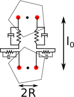
(a)

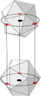
(b)

Figure 1: Setting of cohesive interactions between two particles for a $2D$ system (a) and a $3D$ system (b). Each cohesive interaction is composed of a spring and a damper in compression/tension and shear.

2.2.1 Reaction forces

The cohesive paste between particles is described as an elastic material which can be stretched, compressed and sheared. A cohesive interaction plane, defined for each cohesive interaction, corresponds to the tangential plane normal to the line of unit vector $\boldsymbol{n}$ which connects the two cohesion points. The tangential unit vector $\boldsymbol{t}$ is defined by the tangential deformation. The cohesive reaction forces are computed at cohesion points, and then applied to the center of mass of the particle. Their expression in the reference frame of the cohesive interaction plane is:

$$\boldsymbol{F}=F_{n}\cdot\boldsymbol{n}+F_{t}\cdot\boldsymbol{t},$$

where the normal and the tangential components are respectively given by:

$$F_{n}=-k_{n}^{s}\Delta_{n},$$ (1)

$$F_{t}=-k_{t}^{s}\Delta_{t}.$$ (2)

with $\Delta_{n}$ and $\Delta_{t}$ denoting the compressive/tensile components of the relative displacements in the cohesive interaction plane reference frame, and $k_{n}^{s}$ and $k_{t}^{s}$ the corresponding normal and tangential stiffnesses respectively.

This linear spring model does not dissipate energy. Indeed, in real materials kinetic energy is dissipated by microscopic processes during contact. Therefore we add dissipation by means of viscous damping. The normal and tangential reaction forces become:

$$F_{n}=-k_{n}^{s}\Delta_{n}-k_{n}^{v}U_{n},$$

$$F_{t}=-k_{t}^{s}\Delta_{t}-k_{t}^{v}U_{t},$$

where $U_{n}$, $U_{t}$ denote the relative normal and tangential velocities and $k_{n}^{v}$, $k_{t}^{v}$ the corresponding damping coefficients in normal and tangential directions.

It should be observed that, while tension is opposed solely by cohesive interaction forces, compression may be opposed by both cohesive interaction and contact forces, thus ensuring a transition from elastic to perfectly rigid behaviour in the latter case.

2.2.2 Model parameters

In order to determine the microscopic coefficients $k_{n}^{s}$ and $k_{t}^{s}$, an analogy is done with the continuum elastic modulus of a cohesive paste. Thus, the normal spring stiffness $k_{n}^{s}$ is derived from the Young’s modulus $E_{\mu}$ of a deformable cohesive paste as :

$$k_{n}^{s}=\frac{E_{\mu}S}{l_{0}},$$ (3)

where $S$ is the cohesive interaction surface, which can be viewed as the sectional area of the cohesive paste between the grains divided by the number of cohesive interactions used to model this paste ($2$ in $2D$, $3$ in $3D$). The initial length of a cohesive contact $l_{0}$ is the distance between the two cohesion points when the cohesive interactions are set. Since the cohesive interaction surface $S$ and length $l_{0}$ differ for each pair of particles, a microscopic stiffness heterogeneity is thus introduced. The tangential spring stiffness is determined from the shear modulus, which corresponds to the shear stress to shear strain ratio. By analogy, the force exerted by the tangential spring is assigned a value which balances the force needed to shear the cohesive bond over the tangential displacement $\Delta_{t}$. Hence, the shear modulus may be expressed as:

$$G=\frac{|F_{t}|l_{0}}{S.\Delta_{t}}.$$ (4)

Replacing in Eq. (4) $F_{t}$ by its expression given by Eq. (2) yields the following expression:

$$k_{t}^{s}=\frac{GS}{l_{0}}.$$ (5)

Assuming a perfectly isotropic cohesive paste material, the shear modulus relates to the Young’s modulus $E_{\mu}$ via the Poisson’s ratio $\nu_{\mu}$ according to:

$$G=\frac{E_{\mu}}{2(1+\nu_{\mu})}.$$ (6)

Using Eqs. (3), (5) and (6), the ratio of the normal to tangential stiffnesses may therefore be expressed as follows:

$$\frac{k_{n}^{s}}{k_{t}^{s}}=2(1+\nu_{\mu}).$$ (7)

The damping coefficients $k_{n}^{v}$ and $k_{t}^{v}$ are calculated to obtain a critical damping which prevents oscillations at contact. It has to be noted that the stiffnesses of cohesive interactions are computed once and remain constant until breakage. Thus, damage occurs in the sample only by breakage of cohesive interactions. More sophisticated models such as Cohesive Zone Models (CZM) which take into account the progressive damage of a cohesive contact can be found in (Raous et al., 1999; Rivière et al., 2015).

2.2.3 Breakage of cohesive interactions

We assume that in a cemented material, fracture occurs due to the breakage of the cohesive paste between grains, which corresponds to the rupture of cohesive interactions. Several bond rupture criteria for the DEM modeling of cohesive materials are available in the literature (Jiang et al., 2014; Delenne et al., 2004). In the present work, a cohesive interaction can break only due to tension and/or shear load. When it breaks, the cohesive interaction is no longer able to oppose relative displacement, which is equivalent to setting its stiffnesses ($k_{n}$, $k_{t}$) to zero. However, the two (or three in $3D$) cohesive interactions used to model cohesion between a pair of particles are treated independently : if one breaks, the other one remains intact if not above rupture limit. If all the cohesive interactions between two particles are broken, only contact interaction remains active. Note also that breakage is not reversible in this model : a broken cohesive interaction cannot be restored. Besides, the model incorporates a threshold displacement above which rupture of the cohesion interaction occurs for both tension and shear. For tension, Eqs. (1) and (3) yield:

$$\Delta_{n}^{max}=\frac{l_{0}}{E_{\mu}}\,.\,\sigma_{r}^{n},$$ (8)

and for shear Eqs. (2), (5) and (6) yield:

$$\Delta_{t}^{max}=\frac{2(1+\nu_{\mu})\,l_{0}}{E_{\mu}}\,.\,\sigma_{r}^{t},$$ (9)

with $\sigma_{r}^{n}$ and $\sigma_{r}^{t}$ the strength in tension and shear which are input parameters of the model, taken identical for all the interactions. The threshold displacements have been chosen identical in tension and shear, which implies from Eqs. (8) and (9):

$$\sigma_{r}^{t}=\frac{\sigma_{r}^{n}}{2(1+\nu_{\mu})}$$ (10)

In the following, the rupture threshold will be referred as $\sigma_{r}$, with $\sigma_{r}^{n}=\sigma_{r}$ and $\sigma_{r}^{t}$ given by Eq. (10).

3 2D Benchmark test

3.1 Initial packing

In the following, the approach described above will be applied to a $2D$ benchmark, the uniaxial compression of a rectangular sample composed of polydisperse regular pentagons. The initial packing is built according to the following method. First, discs of average diameter $d$ are deposited under gravity in a rectangular box composed of four rigid walls. The grain diameters are uniformly distributed between $0.5d$ and $1.5d$ to prevent crystallization. Then, each disc is replaced by a regular pentagon which fits exactly inside the disc, with the same arbitrary orientation for all pentagons. The packing is then subjected to a compression phase to increase its solid fraction. This is done by moving the walls at a constant velocity ($V=5.10^{-3}\left[d^{\nicefrac{{3}}{{2}}}\sqrt{\frac{E_{\mu}}{m}}\right]$, see section 3.2.1 for scales), with no other external forces than those applied by the walls (i.e. no gravity). The relative velocities between top/bottom and left/right walls are chosen to achieve the desired height to width aspect ratio of the packing.

Due to the displacement of the walls, the solid fraction can be higher close to the walls than in the packing bulk. To achieve homogenization, the following mixing phase is performed: after a given number of compression time-steps, walls are kept fixed and random velocities are assigned to pentagons. To ensure maximum efficiency of the mixing process, the pentagon/pentagon and pentagon/wall contacts are solved with a full restitution shock law free of friction, so that kinetic energy is not dissipated. Then, all velocities are set to zero and the compression phase resumes.

As soon as the target solid fraction is reached, the compression phase is stopped. All velocities are set to zero and only the locations of particles are kept. Some precautions have to be taken at walls/granular sample contacts during simulations. Indeed, due to the sharp shape of particles, the probability of applying the load to a single particle is high. This could initiate the rupture of the packing at an early stage of the simulation, in an unrealistic manner. To avoid this, the pentagons located at the top and bottom of the packing are smoothed to create a flat wall/packing surface and so to increase the contact surface area with the walls (Fig. 2a).

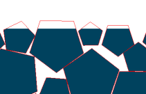
(a)

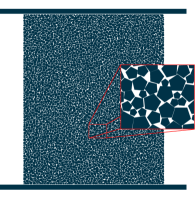
(b)

Figure 2: (a) Smoothing of pentagons in the contact boundary with walls. (b) Typical packing of $5000$ regular pentagons used in compression simulations.

Note that, as expected, due to the building process which introduces randomness, two different packings with the same macroscopic properties (solid fraction, number of particles, size, particle size distribution…) will generally yield differences in the particle structure. For two samples, the orientation distributions of normal unit vectors characterizing contacts as well as cohesive interactions normal unit vector have been plotted in Fig. 3. Although these distributions are similar, small differences are visible between the samples. We can also note that the orientations are fairly isotropically distributed. This packing procedure allows to obtain homogeneous samples (in terms of solid fraction, random orientations, size distribution) while controlling precisely the final aspect ratio and solid fraction, and thus provides a good benchmark for the model. In addition, this random packing of irregular particles can be representative of some common sedimentary rocks such as sandstone (Yang et al., 2013). The results presented in the following have been obtained from simulations using packings of an aspect ratio of $1.2$ constituted of $5000$ regular pentagons, which have been found sufficient to allow good reproductability, as well as reasonable computational cost. Such a packing is presented in Fig. 2b.

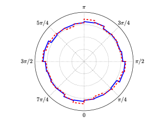
(a)

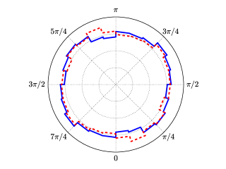
(b)

Figure 3: Orientation distributions of the normal unit vector $\boldsymbol{n}$ for cohesive interactions (a) and contacts (b) obtained for two different initial samples (plain line, dashed line).

Once the initial packing is built, the cohesive interactions have to be set inside the modeled material. As cohesion is active even if particles are not touching, a criterion is required to decide whether two particles share a cohesion interaction or not. A rather simple way to do this is to define an interaction range (Hentz et al., 2004a) for cohesive effects, so that if the distance between two particles is below this range cohesion will act. However, this requires an additional model parameter, which needs to be added to the calibration procedure. Another method, which is the one used in this work, consists in determining the list of particles interacting through cohesive bonds by computing a Delaunay triangulation from the centers of all particles. Each edge of the triangulation corresponds to a pair of particles undergoing cohesive interaction. This choice is not insignificant because it leads to a constant number of cohesive interactions per grain (Gervois et al., 1995) and thus it may mitigate the effect of the solid fraction (see discussion in Section 3.2.3). For each cohesive interaction, two (in $2D$) or three (in $3D$) cohesion points are placed according to the rules defined at the beginning of section 2.2. The distance $R$ between cohesion points and center of the particles is chosen as the average radius $r$ (the radius of a disc of same area than the pentagon) of the smallest pentagon of the pair of particles enduring a cohesive interaction. A heterogeneity terms of $R$ values is thus introduced for polydisperse packings, and thus only the $R/r$ ratio is a constant input parameter for all cohesive interactions. A discussion on the influence of $R$ is provided in section 3.2.6. Once the cohesion is set, the lateral walls are removed and the packing is then ready for loading.

3.2 Uniaxial Compression

Uniaxial compression tests have been performed on different packings by moving a wall at constant velocity $V_{c}$ while maintaining the other wall fixed. The sample is submitted only to external forces applied by these walls in the absence of gravity. The compression velocity is chosen sufficiently low to ensure quasi-static equilibrium and avoid unexpected material responses such as initiation of rupture near a wall. The quasi-static equilibrium is checked by comparing the stresses applied by the two loading walls.

3.2.1 Simulation parameters

The obtained macroscopic behavior is controlled by microscopic contact and cohesive interaction parameters. Those used in our simulations are made dimensionless using the following scaling rules :

• Mass scale : mean mass $m$ of particles

• Length scale : mean equivalent diameter $d$ of pentagons, defined as the diameter of a disc with the same surface area as the pentagon

• Time scale : $t_{0}=\sqrt{\frac{m}{E_{\mu}d}}$, so that the stress scale is Young’s modulus $E_{\mu}$ of the cohesive paste.

As the Young’s modulus $E_{\mu}$ is that of a cohesive paste, it is taken identical for all cohesive interactions, with $E_{\mu}=1$ according to the chosen stress scale. The Poisson’s ratio of the modeled cohesive paste is taken as $\nu_{\mu}=0.25$. The stiffness heterogeneity of cohesive interactions originates from geometrical properties ($S$, $l_{0}$). Friction coefficients at particle/particle $\mu_{pp}$ and wall/particle $\mu_{pw}$ contacts are set to $0.3$ and $0.5$ respectively. The stress threshold in tension is assigned a value of $\sigma_{r}^{n}=5.10^{-3}$, and thus following Eq. (10) the stress threshold in shear is set to $\sigma_{r}^{t}=2.10^{-3}$. Finally, the compression velocity is $V_{c}=2.10^{-5}$.

The choice of the time-step $dt$ is important as it guarantees the precision and the stability of the computation. It has to be sufficiently small compared to all time scales, including the damping characteristic time of particles motion, but also not too small to allow reasonable simulation duration time. A dimensionless time-step value of $10^{-1}$ is considered a good compromise between precision and simulation duration. Usually simulations require $50000$ to $100000$ time-steps to achieve rupture of the packing, depending on the value of cohesive interaction parameters, especially the cohesive interaction strength.

3.2.2 Macroscopic behavior

The typical stress/strain curve obtained for uniaxial compression tests is presented in Fig. 4a together with the variations of the number of broken cohesive interactions. During the first phase of compression, the material clearly exhibits a linear elastic behavior characterized by the linear part of the stress-strain curve. During this phase, the cohesive interactions store the increasing strain energy applied to the packing by the walls. The modeled packing being initially consolidated, it doesn’t exhibit a non-linear increase of stiffness for small deformations as can be seen in experiments due to closure of pores or small rearrangements of grains (Wawersik and Fairhurst, 1970).

Then, the stress supported by some cohesive interactions exceeds the elastic limit $\sigma_{r}$ and they break. These breakages induce small drops in the macroscopic stress and the stress-strain curve starts to deviate slightly form the linear behavior. Suddenly, when a critical strain $\epsilon_{p}$ is reached, large amounts of cohesive interactions break: this leads to a major drop of the stress-strain curve, and the emergence and propagation of a macroscopic crack across the packing. Although the propagation of the macroscopic crack is very fast, as we will show, this phenomenon is progressive.

Figure 4b shows the spatial distribution of broken cohesive interactions at different stages of the compression. Initially, the cohesive interactions seem to break more or less randomly across the packing but then just before the peak (II) we observe a localization and the appearance of a crack path. Moreover, the post-peak region exhibits several minor peaks which correspond to the extension of the macroscopic crack or the initiation of a new one. The fracture planes align with the diagonals of the sample, forming two fracture cones near the walls. This fracture pattern agrees qualitatively well with experiments of real cohesive materials under uniaxial compression with frictional platens (Jaeger et al., 2007). However, a different boundary condition (e.g. frictionless walls) would yield a different fracture pattern (D’Addetta et al., 2002).

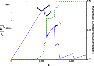
(a)

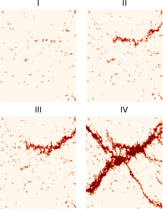
(b)

Figure 4: (a) Stress/strain curve (blue solid line) obtained together with the cumulative share of broken cohesive interactions (green dashed line). (b) Broken cohesive interactions at different stages of the compression. The localization of cohesive interactions breakage and progressive behavior of fracture is clearly seen.

3.2.3 Influence of the initial solid fraction

Different initial packing characteristics yield differences in the modeled microstructure, and so an expected different macroscopic behavior. An important packing characteristic is the solid fraction of the sample. Increasing the solid fraction leads to an increase of the density of cohesive interactions in the sample, but also to a decrease of the cohesive interaction length $l_{0}$ since particles are closer to one another. According to Eq. (3), decreasing $l_{0}$ will increase the cohesive interaction stiffnesses and so influence the macroscopic stiffness as well. For results presented below, the macroscopic Young’s modulus is determined as the slope of a fit of the linear part of the stress/strain curve corresponding to the linear elastic regime. Figure 5 shows the macroscopic Young’s modulus $E_{M}$ obtained for discrete solid fraction values ranging between $0.6$ and $0.84$. As expected, increasing the solid fraction leads to an increase of macroscopic Young’s modulus, up to $40\%$ in the studied range. It is clear that solid fraction is an important parameter which controls the macroscopic stiffness of the modeled material. Note also that as cohesive interactions are set according to a Delaunay triangulation from the center of particles, the average coordination number of $6$ for $2D$ packings remains the same whatever the solid fraction (Gervois et al., 1995). Determining the cohesive neighborhood with another method may lead to a different effect of the solid fraction.

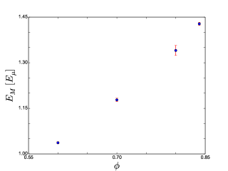
Figure 5: Macroscopic Young’s modulus $E_{M}$ measured for solid fraction $\phi$ ranging from $0.6$ to $0.84$.

3.2.4 Influence of cohesive interactions coordination number

As described before, the Delaunay triangulation used to establish the cohesive interactions network leads in $2D$ to a cohesive interactions coordination number $z=6$. In order to study the influence of smaller $z$ on the macroscopic behavior, cohesive interactions have been randomly removed from the sample. The stress-strain curves for $z=$ $6$, $5$ ,$4$ and $3$ obtained for samples of solid fraction $\phi=0.84$ are presented in Fig. 6. A linear decrease of $z$ leads to a linear decrease of the macroscopic Young’s modulus because less cohesive interactions contribute to the overall stiffness of the sample. Therefore, the same strain energy is endured by fewer cohesive interactions and so the fracture will occur for a lower stress peak. Moreover, the cohesive interactions coordination number has a strong influence on the post-peak behavior. Indeed, the amplitude of the secondary peaks decreases with $z$, and so does the residual stiffness in the post peak region. This means that a smaller $z$ leads to a loss of brittleness. The spatial distribution of broken cohesive interactions at the final stage of the simulation ($\epsilon=0.009$) is plotted in Fig. 7. For small $z$, it appears clearly that the breakage of cohesive interactions is no more localized on identified planes. The loss of brittleness is thus caused by the emergence of a number of small cracks instead of macroscopic fractures inside the sample.

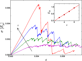
Figure 6: Stress/strain curves obtained for values of the cohesive interactions coordination number $z$ increasing from $3$ to $6$. Insert : macroscopic Young’s modulus $E_{M}$ versus $z$. Error bars are smaller than the line thickness.

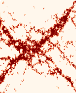
(a)

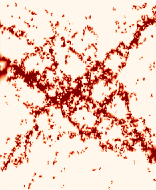
(b)

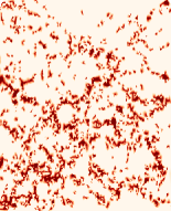
(c)

Figure 7: Broken cohesive interactions at $\epsilon=0.009$ for different cohesive interactions coordination numbers : (a) $z=5$, (b) $z=4$, (c) $z=3$. A loss of localization for small $z$ is observed.

3.2.5 Influence of contact friction

In order to evaluate the influence of the particle-particle contact friction coefficient on the macroscopic Young’s modulus $E_{M}$, several simulations have been performed for values of $\mu_{pp}$ ranging from $0$ to $0.7$ and sample solid fraction values of $0.6$, $0.7$ and $0.84$ (Fig. 8a). By introducing friction between particles, reaction forces opposing sliding contribute to the global resistance of the sample. Increasing the friction coefficient then yields an increase of the macroscopic Young’s modulus characteristic of the macroscopic stiffness of the material. This effect is stronger for higher solid fraction values since increasing the solid fraction also increases the density of particles contacts. However, this effect is rather small (less than $4\%$) compared to that of the solid fraction. Indeed, even with a solid fraction of $0.84$, the ratio of the number of contacts to the number of cohesive interactions is small ($\simeq 2\%$), so energy dissipation due to contact friction has a weak influence on macroscopic Young’s modulus.

The macroscopic Poisson’s ratio $\nu_{M}$, quantifying the dilatational strain under compression of the modeled material, has been determined by considering a centrally located horizontal slice whose thickness is $20\%$ of the sample total height. This slice is then split into $20$ sub-slices of equal thickness, whose mean horizontal strain may easily be calculated. The Poisson’s ratio is then determined as the slope of the fit of the vertical strain / horizontal strain curve. Figure 8b shows the measured $\nu_{M}$ for for different values of the solid fraction and friction coefficient. The values of $\nu_{M}$ vary from $0.145$ to almost $0.2$ in the range of studied parameters. They increase with the solid fraction, which denotes a non negligible effect of contact between particles on their transverse displacement. Indeed, when two pentagons are compressed, the polygonal shape promotes sliding along radial directions, which contribute to dilatancy of the material. The friction coefficient also affects $\nu_{M}$, by opposing lateral displacement via energy dissipation. The Poisson’s ratio is thus higher for small values of $\mu_{pp}$. This effect is weaker for lower solid fraction values and seems to saturate for $\mu_{pp}$ greater than $0.3$.

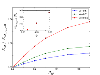
(a)

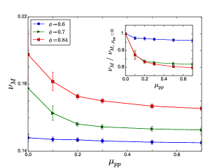
(b)

Figure 8: (a) Influence of the friction coefficient between pentagons on the macroscopic Young’s modulus for different solid fraction values. Macroscopic Young’s modulus for each solid fraction has been normalized by its value for $\mu_{pp}=0$ to highlight the influence of the friction coefficient. This effect is small although it increases with the solid fraction. Insert: Young’s modulus for $\mu_{pp}=0$ versus the solid fraction. It increases as explained in section 3.2.3. (b) Macroscopic Poisson’s ratio $\nu_{M}$ for the same values of $\phi$ and $\mu_{pp}$ than (a). Insert : $\nu_{M}$ normalized by $\nu_{M},\,\mu_{pp}=0$.

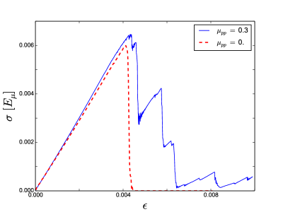
Figure 9: Stress/strain curves for contact friction values $\mu_{pp}=0$ (red dots) and $\mu_{pp}=0.3$ (blue) for the same sample of solid fraction $\phi=0.84$. The different post-peak behaviors are clearly seen.

Although the effect of the contact friction coefficient is rather small in the elastic part, it has a strong influence on the post peak behavior (Fig. 9). Indeed, with a friction coefficient of $0.$, the stress falls suddenly to zero after having reached the stress peak, which means that the fracture propagates quickly through the sample. Contrariwise, a different behavior is observed with a contact friction coefficient of $0.3$. First, the fracture initiates and the stress drops. Then, we observe a stress increase until it reaches a new peak lower than the main one. This means that the energy dissipation due to contact friction influences the fracture propagation across the sample, and so its strength in the post-peak region.

3.2.6 Influence of the ratio $R/r$

To introduce resistance to relative rotation for cohesive interactions, two ($2D$) or three ($3D$) cohesion points are placed at a distance $R$ of the center of each particle. For $R\neq\,0$, a relative rotation of the pentagons will induce a reaction torque, which increases with $R$ and so we expect an increase of macroscopic stiffness of the modeled material. As described before, $R$ has been chosen as the average radius $r$ of the smallest pentagon of the pair, thus $R/r=1$ for all cohesive interactions. Figure 10 shows the measured macroscopic Young’s modulus for values of the ratio $R/r$ ranging from $0$ (no resistance to rotation) to $2$. It can be clearly seen that the ratio $R/r$ has a strong effect on the macroscopic Young’s modulus, up to an increase by $20\%$ in the studied range, which also indicates that relative rotations are not negligible even for a solid fraction of $0.84$ as presented in Fig. 10. However, the effect seems to saturate for values of $R/r$ above $1$ in this case. The ratio $R/r$ is thus a simple model parameter allowing to control the resistance of rotation between cohesive pairs of particles, and thus its influence on macroscopic stiffness of the material.

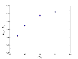
Figure 10: Macroscopic Young’s moduli $E_{M}$ for values of the ratio $R/r$ ranging from $0$ to $2$, for samples of solid fraction $\phi=0.84$.

3.2.7 Influence of cohesive interactions rupture threshold

The macroscopic fracture of the material is only due to the rupture of cohesive interactions between particles. Thus, the rupture threshold $\sigma_{r}$ is expected to have a strong influence on the strength of the modeled material. Simulations for different rupture threshold values have been performed, and the corresponding stress/strain behaviors are plotted in Fig. 11a. As expected, the rupture threshold of cohesive interactions controls the peak stress $\sigma_{peak}$ and peak strain $\epsilon_{peak}$ of the packing and so the resistance of the material. However, it has no influence on the slope of the elastic part of the stress-strain curves because no cohesive interaction undergoes a stress as high as $\sigma_{r}$ during this phase. The stress threshold also seems to change the post peak regime by influencing the crack propagation, as can be seen in Fig. 11b. The secondary peaks observed for simulations with $\sigma_{r}=5.10^{-3}$ are reduced with decreasing $\sigma_{r}$, and disappear for $\sigma_{r}=2.10^{-4}$. Indeed when a crack initiates, weaker cohesive interactions will make it easier to propagate across the sample. On the contrary, stronger cohesive interactions stop the crack earlier and propagation of the fracture will restart only when the strain energy becomes sufficient again to break other cohesive interactions. In the case of very weak cohesive interactions ($\sigma_{r}=2.10^{-4}$), the absence of secondary peaks means that the first crack has enough energy to percolate across the sample on its first try. This effect is superimposes with that of contact friction described before to influence the propagation of the rupture through the material.

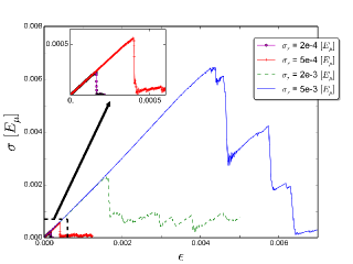
(a)

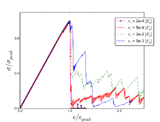
(b)

Figure 11: (a) Stress-strain behavior obtained for increasing cohesive interaction rupture threshold. (b) Same as (a) but with the stress $\sigma$ and axial strain $\epsilon$ normalized by values at peak ($\sigma_{peak}$,$\epsilon_{peak}$) to see the effect of the stress threshold on post-peak behavior.

4 Conclusion

We have presented a mixed model combining NSCD description for contact behavior and cohesive interactions made of pairs of cohesion points to mimic a cohesive phase lying between the particles of a rock piece. The use of cohesion points allows to deal with particles of complex shapes, and also to model cohesive materials of various solid fraction values up to 1. The model was tested in $2D$, where an aggregate grain was modeled as a polydisperse packing of polygons, bounded by cohesive interactions in order to mimic the presence of cohesive bridges, as can be found in real materials.

The model has proven to mimic the overall macroscopic behavior of an aggregate grain subjected to axial compression. A linear elastic behavior during which cohesive interactions remain intact is followed by a sudden drop of stress on walls corresponding to the initiation and propagation of macroscopic fractures inside the packing, characteristic of a brittle material. Energy dissipation due to contact friction has an important impact on the propagation of fractures across the sample and induces progressive failure behavior. The microscopic elastic limit allows to control the strength of the modeled material without acting on the elastic slope of the response. As higher microscopic elastic limit values require more energy to break cohesive interactions, the fracture propagation is also influenced. The cohesive interactions coordination number $z$ has an influence on both elastic and post-peak behavior. Indeed, decreasing $z$ leads to a decrease of macroscopic stiffness and has also an effect on breakage localization of cohesive interactions. Finally, the solid fraction of the packing has been studied and shows a direct effect on the macroscopic Young’s modulus and thus on the stiffness of the material.

The method used to model cohesion can be applied to any particle shape in $2D$ and $3D$. Therefore, further studies will be carried out, especially to quantify the influence of particle shapes for other non regular polygons, closer to real material. The model will then be tested for $3D$ simulations.

References

References

- Affes et al. (2012) Affes, R., Delenne, J. Y., Monerie, Y., Radjaï, F., Topin, V., 2012. Tensile strength and fracture of cemented granular aggregates. European Physical Journal E 35 (11).
- André et al. (2012) André, D., Iordanoff, I., Charles, J.-l., Néauport, J., 2012. Discrete element method to simulate continuous material by using the cohesive beam model. Computer Methods in Applied Mechanics and Engineering 213-216, 113–125.
- Asahina et al. (2011) Asahina, D., Bolander, J. E., 2011. Voronoi-based discretizations for fracture analysis of particulate materials. Powder Technology 213, 92–99.
- Berton et al. (2006) Berton, S., Bolander, J. E., 2006. Crack band model of fracture in irregular lattices. Comput. Methods Appl. Mech. Engrg. 195, 7172–7181.
- Bolander et al. (2005) Bolander, J. E., Sukumar, N., 2005. Irregular lattice model for quasistatic crack propagation. Physical Review B 71 (094106), 1–12.
- Bolton et al. (2004) Bolton, M. D., Nakata, Y., Cheng, Y. P., 2004. Crushing and plastic deformation of soils simulated using DEM. Géotechnique 54 (2), 131–141.
- Bolton et al. (2008) Bolton, M. D., Nakata, Y., Cheng, Y. P., 2008. Micro- and macro-mechanical behaviour of DEM crushable materials. Géotechnique 58 (6), 471–480.
- Brown et al. (2014) Brown, N. J., Chen, J.-F., Ooi, J. Y., 2014. A bond model for DEM simulation of cementitious materials and deformable structures. Granular Matter 16 (3), 299–311.
- Cheng et al. (2003) Cheng, Y. P., Bolton, M. D., Nakata, Y., 2003. Discrete element simulation of crushable soil. Géotechnique 53 (7), 633–641.
- Cho et al. (2007) Cho, N., Martin, C., Sego, D., 2007. A clumped particle model for rock. International Journal of Rock Mechanics and Mining Sciences 44 (7), 997–1010.
- D’Addetta et al. (2002) D’Addetta, G. A., Kun, F., Ramm, E., 2002. On the application of a discrete model to the fracture process of cohesive granular materials. Granular Matter 4 (2), 77–90.
- Delenne et al. (2004) Delenne, J.-Y., El Youssoufi, M. S., Cherblanc, F., Bénet, J.-C., 2004. Mechanical behaviour and failure of cohesive granular materials. Int. J. Numer. Anal. Meth. Geomech. 28 (15), 1577–1594.
- Galindo-Torres et al. (2012) Galindo-Torres, S., Pedroso, D., Williams, D., Li, L., 2012. Breaking processes in three-dimensional bonded granular materials with general shapes. Computer Physics Communications 183 (2), 266–277.
- Gervois et al. (1995) Gervois, A., Annic, C., Lemaitre, J., Ammi, M., Oger, L., Troadec, J.-P. P., 1995. Arrangement of discs in 2d binary assemblies. Physica A 218 (3-4), 403–418.
- Hentz et al. (2004a) Hentz, S., Daudeville, L., Donzé, F. V., 2004a. Identification and Validation of a Discrete Element Model for Concrete. J. Eng. Mech. 130 (6), 709–719.
- Hentz et al. (2004b) Hentz, S., Donzé, F. V., Daudeville, L., 2004b. Discrete element modelling of concrete submitted to dynamic loading at high strain rates. Computers & Structures 82 (29-30), 2509–2524.
- Jaeger et al. (2007) Jaeger, J. C., Cook, N., Zimmerman, R., 2007. Fundamentals of Rock Mechanics. In: Fundamentals of Rock Mechanics. Blackwell Publishing, pp. 87–90.
- Jean (1999) Jean, M., 1999. The non-smooth contact dynamics method. Comput. Methods Appl. Mech. Engrg. 177 (3-4), 235–257.
- Jiang et al. (2014) Jiang, M., Liu, F., Zhou, Y., 2014. A bond failure criterion for DEM simulations of cemented geomaterials considering variable bond thickness. Int. J. Numer. Anal. Meth. Geomech.
- Jiang et al. (2006) Jiang, M. J., Yu, H. S., Harris, D., 2006. Bond rolling resistance and its effect on yielding of bonded granulates by DEM analyses. International Journal for Numerical and Analytical Methods in Geomechanics 30 (8), 723–761.
- Jing (2003) Jing, L., 2003. A review of techniques, advances and outstanding issues in numerical modelling for rock mechanics and rock engineering. International Journal of Rock Mechanics and Mining Sciences 40 (3), 283–353.
- McDowell and Bolton (1998) McDowell, G. R., Bolton, M. D., 1998. On the micromechanics of crushable aggregates. Géotechnique 48 (5), 667–679.
- Moreau (1988) Moreau, J. J., 1988. Unilateral contact and dry friction in finite freedom analysis, cism cours Edition. Vol. 302. Springer-Verlag, Wien, New York.
- Nguyen et al. (2015) Nguyen, D.-h., Azéma, E., Sornay, P., Radjaï, F., 2015. Bonded-cell model for particle fracture. Physical Review E 91 (022203), 1–9.
- Potyondy and Cundall (2004) Potyondy, D. O., Cundall, P. A., 2004. A bonded-particle model for rock. International Journal of Rock Mechanics and Mining Sciences 41 (8), 1329–1364.
- Raous et al. (1999) Raous, M., Cangémi, L., Cocu, M., 1999. A consistent model coupling adhesion, friction, and unilateral contact. Computer Methods in Applied Mechanics and Engineering 177 (3-4), 383–399.
- Renouf et al. (2004) Renouf, M., Dubois, F., Alart, P., 2004. A parallel version of the non smooth contact dynamics algorithm applied to the simulation of granular media. Journal of Computational and Applied Mathematics 168 (1-2), 375–382.
- Rivière et al. (2015) Rivière, J., Renouf, M., Berthier, Y., 2015. Thermo-Mechanical Investigations of a Tribological Interface. Tribology Letters 58 (3).
- Scholtès and Donzé (2013) Scholtès, L., Donzé, F.-V., 2013. A DEM model for soft and hard rocks: Role of grain interlocking on strength. Journal of the Mechanics and Physics of Solids 61 (2), 352–369.
- Spettl et al. (2015) Spettl, A., Dosta, M., Antonyuk, S., Heinrich, S., Schmidt, V., 2015. Statistical investigation of agglomerate breakage based on combined stochastic microstructure modeling and DEM simulations. Advanced Powder Technology 26 (3), 1021–1030.
- Wawersik and Fairhurst (1970) Wawersik, W. R., Fairhurst, C., 1970. A study of brittle rock fracture in laboratory compression experiments. Int. J. Rock Mech. Min. Sci. 7, 561–575.
- Weerasekara et al. (2013) Weerasekara, N., Powell, M., Cleary, P., Tavares, L., Evertsson, M., Morrison, R., Quist, J., Carvalho, R., 2013. The contribution of DEM to the science of comminution. Powder Technology 248, 3–24.
- Yang et al. (2013) Yang, Y. S., Liu, K. Y., Mayo, S., Tulloh, A., Clennell, M. B., Xiao, T. Q., 2013. A data-constrained modelling approach to sandstone microstructure characterisation. Journal of Petroleum Science and Engineering 105, 76–83.
- Zhao et al. (2015) Zhao, T., Dai, F., Xu, N. W., Liu, Y., Xu, Y., 2015. A composite particle model for non-spherical particles in DEM simulations. Granular Matter 17 (6), 763–774.