Global and local statistics in turbulent convection at low Prandtl numbers

Abstract

Statistical properties of turbulent Rayleigh-Bénard convection at low Prandtl numbers $Pr$, which are typical for liquid metals such as mercury or gallium ($Pr\simeq 0.021$) or liquid sodium ($Pr\simeq 0.005$), are investigated in high-resolution three-dimensional spectral element simulations in a closed cylindrical cell with an aspect ratio of one and are compared to previous turbulent convection simulations in air for $Pr=0.7$. We compare the scaling of global momentum and heat transfer. The scaling exponent $\beta$ of the power law $Nu=\alpha Ra^{\beta}$ is $\beta=0.265\pm 0.01$ for $Pr=0.005$ and $\beta=0.26\pm 0.01$ for $Pr=0.021$, which are smaller than that for convection in air ($Pr=0.7$, $\beta=0.29\pm 0.01$). These exponents are in agreement with experiments. Mean profiles of the root-mean-square velocity as well as the thermal and kinetic energy dissipation rates have growing amplitudes with decreasing Prandtl number which underlies a more vigorous bulk turbulence in the low–$Pr$ regime. The skin-friction coefficient displays a Reynolds-number dependence that is close to that of an isothermal, intermittently turbulent velocity boundary layer. The thermal boundary layer thicknesses are larger as $Pr$ decreases and conversely the velocity boundary layer thicknesses become smaller. We investigate the scaling exponents and find a slight decrease in exponent magnitude for the thermal boundary layer thickness as $Pr$ decreases, but find the opposite case for the velocity boundary layer thickness scaling. A growing area fraction of turbulent patches close to the heating and cooling plates can be detected by exceeding a locally defined shear Reynolds number threshold. This area fraction is larger for lower $Pr$ at the same $Ra$, but the scaling exponent of its growth with Rayleigh number is reduced. Our analysis of the kurtosis of the locally defined shear Reynolds number demonstrates that the intermittency in the boundary layer is significantly increased for the lower Prandtl number and for sufficiently high Rayleigh number compared to convection in air. This complements our previous findings of enhanced bulk intermittency in low-Prandtl-number convection.

1 Introduction

Many turbulent thermal convection phenomena in nature and technology are present in low–Prandtl–number fluids for which the kinematic viscosity of the fluid, $\nu$, is much smaller than the thermal diffusivity of the temperature field, $\kappa$, or in other words for which the ratio of both, the Prandtl number

$$Pr=\frac{\nu}{\kappa}\,.$$ (1)

is much smaller than one. Applications range from turbulent convection in the Sun (Hanasoge et al. (2015)) or the liquid metal core of the Earth (King & Aurnou (2013)) to nuclear engineering (Grötzbach (2013)) or liquid metal batteries (Kelley & Sadoway (2014)). In all these examples $Pr\lesssim 2\times 10^{-2}$, and in the solar convection case it could be smaller than $Pr\sim 10^{-4}$. Convective turbulence in these examples appears mostly in combination with other physical processes, such as rotation, radiation or the generation of magnetic fields. Rayleigh-Bénard convection (RBC), a fluid flow in a layer which is cooled from above and heated from below, is the simplest example of a turbulent convective flow.

The record of experimental and numerical data for low-Prandtl-number convection is much smaller than for convection in air or water. Laboratory experiments are challenging in several ways. For Prandtl numbers $Pr<0.2$, opaque liquid metals such as liquid mercury or gallium at $Pr\simeq 0.025$ (Rossby (1969); Cioni et al. (1996, 1997); Takeshita et al. (1996); Glazier et al. (1999); Aurnou & Olson (2001); King & Aurnou (2013)) or liquid sodium at $Pr\simeq 0.005$ (Horanyi et al. (1999); Cioni et al. (1997a); Frick et al. (2015)) have to be used. Additionally, experiments in sodium require working temperature of more than 100$\,{}^{\circ}$C. An optical access to the flow by laser-imaging techniques is impossible. The heating and cooling at the bottom and top walls is usually established with copper plates. In liquid sodium experiments, the thermal conductivity of the plates is thus not significantly higher than that of the working fluid. This introduces significant variations of the temperature at the plates and can alter the magnitude of the heat transfer since the boundary conditions will be a mixture of prescribed temperature and prescribed normal temperature derivative, known as Robin boundary conditions. For an experimental analysis we refer to Horanyi et al. (1999). In low-Prandtl number convection the thermal boundary layer at the solid heating and cooling plates is much thicker than the velocity boundary layer. This has important implications for the turbulent heat and momentum transfer which is one focus of the research in turbulent convection (e.g. in Grossmann & Lohse (2000); Chillà & Schumacher (2012); Scheel & Schumacher (2014)). The global heat transfer is quantified by the dimensionless Nusselt number, $Nu$, while the global momentum transfer is measured by the Reynolds number, $Re$. Detailed definitions of both parameters are given in section 2.1. Both the Nusselt and Reynolds numbers are functions of the Prandtl number $Pr$ and a second dimensionless parameter which quantifies the thermal driving of the turbulence, namely the Rayleigh number $Ra$. Different scaling laws $Nu(Ra)$ have been reported in different convection experiments for mercury and gallium, i.e., at fixed Prandtl number. In liquid sodium, only one experimental data record by Horanyi et al. (1999) exists which is similar to the parameters in this paper. This discussion implies that direct numerical simulations (DNS) are important for gaining access to the full three-dimensional turbulent fields in low-$Pr$ convection and to assure the accuracy of the boundary conditions.

In the present work, we study the local and global statistical properties of turbulent convection flows at very low Prandtl numbers as present in liquid mercury and liquid sodium. We analyze a series of very high-resolution DNS obtained for moderate Rayleigh numbers in a cylindrical cell with an aspect ratio of one. We obtain global scaling laws for the turbulent heat and momentum transfer and compare our findings with available data as well as the scaling theory of Grossmann & Lohse (2001) and a recent update by Stevens et al. (2013). In addition, we analyze the turbulence statistics for a series of three DNS runs which have been conducted at different Rayleigh and Prandtl numbers but with the same Grashof number $Gr=Ra/Pr$ for all three runs (for definition see section 2.2). This perspective (Schumacher et al. (2015)) leaves the dimensionless Navier-Stokes equations unchanged and thus provides a more consistent comparison of convective flow at different Prandtl numbers from the point of view of fluid turbulence.

A second focus of the present work is a detailed local statistical analysis of the dynamics in the boundary layers of velocity and temperature fields. While the heat transport is reduced in low–$Pr$ convection, production of vorticity and shear are strongly enhanced, both in the bulk and in the boundary layers. This is the reason why simulations of turbulent convection at very low Prandtl numbers become very demanding, as is reported for homogeneous turbulent flows (Mishra & Verma (2010)), in planar turbulent flows between parallel free-slip or no-slip walls (Kerr & Herring (2000); Breuer et al. (2004); Verma et al. (2012); Petschel et al. (2013)) or in closed cylindrical cells (Camussi & Verzicco (1998); van der Poel et al. (2013); Schumacher et al. (2015)). We focus our interest on the boundary layer dynamics and determine that the enhanced intermittency in the bulk is connected to a stronger intermittent behavior in the boundary layer, in particular for the velocity field. But, while the vorticity and shear are enhanced in low Prandtl number convection, we also find that the scaling of many diagnostic quantities is weaker. We postulate that this is due to the reduced heat transport and weaker dependence of the Nusselt number on the Rayleigh number.

The outline of the paper is as follows. In the next section, we present the model equations, the numerical method and the data sets. The third section discusses the scaling laws for global heat and momentum transfer. Section 4 turns to the statistics at constant Grashof number and is followed by a detailed boundary-layer analysis in section 5. Finally we summarize our findings and give a brief outlook for future work.

2 Numerical model

2.1 Equations of motion

We solve the three-dimensional equations of motion in the Boussinesq approximation. The equations are made dimensionless by using height of the cell $H$, the free-fall velocity $U_{f}=\sqrt{g\alpha\Delta TH}$ and the imposed temperature difference $\Delta T$. The equations contain the three control parameters: the Rayleigh number $Ra$, the Prandtl number $Pr$ and the aspect ratio $\Gamma=D/H$ with the cell diameter $D$. The equations are given by

$${\bm{\nabla}}\cdot{\bf u} = 0\,,$$ (2)

$$\frac{\partial{\bf u}}{\partial t}+({\bf u}\cdot{\bm{\nabla}}){\bf u} = -{\bm{\nabla}}p+\sqrt{\frac{Pr}{Ra}}{\bm{\nabla}}^{2}{\bf u}+T{\bf e}_{z}\,,$$ (3)

$$\frac{\partial T}{\partial t}+({\bf u}\cdot{\bm{\nabla}})T = \frac{1}{\sqrt{RaPr}}{\bm{\nabla}}^{2}T\,,$$ (4)

where

$$Ra=\frac{g\alpha\Delta TH^{3}}{\nu\kappa}\,,\;\;\;\;\;\;\;\;Pr=\frac{\nu}{\kappa}\,.$$ (5)

The free-fall Reynolds number $Re_{f}$ is given by

$$Re_{f}=\frac{U_{f}H}{\nu}=\sqrt{\frac{Ra}{Pr}}\,.$$ (6)

The variable $g$ stands for the acceleration due to gravity, $\alpha$ is the thermal expansion coefficient, $\nu$ is the kinematic viscosity, and $\kappa$ is thermal diffusivity. We use an aspect ratio of $\Gamma=1$ here. No-slip boundary conditions for the fluid (${\bf u}=0$) are applied at the walls. The side walls are thermally insulated ($\partial T/\partial{\bf n}=0$) and the top and bottom plates are held at constant dimensionless temperatures $T=0$ and 1, respectively. In response to the input parameters $Ra$, $Pr$ and $\Gamma$, turbulent heat and momentum fluxes are established. The turbulent heat transport is determined by the Nusselt number which is defined as

$$Nu=1+\sqrt{RaPr}\langle u_{z}T\rangle_{V,t}\,.$$ (7)

The turbulent momentum transport is expressed by the Reynolds number which is defined as

$$Re=u_{rms,V}\sqrt{\frac{Ra}{Pr}}=u_{rms,V}Re_{f}\;\;\;\;\text{with}\;\;\;\;u_{rms,V}=\sqrt{\langle u_{i}^{2}\rangle_{V,t}}\,,$$ (8)

In both definitions $\langle\cdot\rangle_{V,t}$ stands for a combined volume and time average.

The equations are numerically solved by the Nek5000 spectral element method package which has been adapted to our problem. The code employs second-order time-stepping, using a backward difference formula. The whole set of equations is transformed into a weak formulation and discretized with a particular choice of spectral basis functions (Fischer 1997, Deville et al. 2002). The resulting linear, symmetric Stokes problem is solved implicitly. This system is split, decoupling the viscous and pressure steps into independent symmetric positive definite subproblems which are solved either by Jacobi (viscous) or multilevel Schwartz (pressure) preconditioned conjugate gradient iteration. Fast parallel solvers based on direct projection or more scalable algebraic multigrid are used for the coarse-grid solve that is part of the pressure preconditioner. For further numerical details and comprehensive tests of the sufficient spectral resolution, we refer to detailed investigations in Scheel et al. (2013).

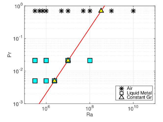
Figure 1: (Colour online) Prandtl number-Rayleigh number parameter space. The solid diagonal line corresponds to data at constant Grashof number. The different working fluids are indicated in the legend. The data for air are from Scheel & Schumacher (2014).

Run	$Ra$	$Pr$	$N_{e}$	$N$	$N_{bl}$	$Nu$	$\delta_{T}/H$	$u_{rms}$	$Re$
1	$3.33\times 10^{8}$	0.7	875,520	11	40	$44.9\pm 1.6$	0.011	$0.171\pm 0.003$	$3720\pm 60$
2	$3\times 10^{5}$	0.021	256,000	7	54	$4.29\pm 0.12$	0.117	$0.483\pm 0.009$	$1830\pm 30$
3	$10^{6}$	0.021	256,000	9	48	$5.43\pm 0.03$	0.093	$0.439\pm 0.006$	$3030\pm 40$
4	$10^{7}$	0.021	875,520	11	26	$10.11\pm 0.05$	0.050	$0.387\pm 0.005$	$8450\pm 100$
5	$10^{8}$	0.021	2,374,400	13	18	$19.1\pm 1.3$	0.026	$0.332\pm 0.004$	$22900\pm 300$
6	$3\times 10^{5}$	0.005	256,000	9	43	$3.26\pm 0.02$	0.153	$0.597\pm 0.003$	$4620\pm 20$
7	$10^{6}$	0.005	875,520	9	39	$4.45\pm 0.07$	0.112	$0.586\pm 0.003$	$8290\pm 40$
8	$2.38\times 10^{6}$	0.005	2,374,400	11	30	$5.66\pm 0.09$	0.088	$0.590\pm 0.006$	$12800\pm 120$

Table 1: Parameters of the different spectral element simulations. We show the Rayleigh number $Ra$, the Prandtl number $Pr$, the total number of spectral elements $N_{e}$, the polynomial order $N$, and the number of grid points inside the velocity boundary layer, $N_{bl}$. The latter is calculated by (21). We also show the Nusselt number $Nu$ (see (7)), the thermal boundary layer thickness $\delta_{T}$ (see (23)), the root-mean-square velocity ${u}_{rms}$, and the Reynolds number $Re$ (see (8)). The error bars have been obtained by evaluating the results over the first and second halves of the corresponding data set separately and taking the difference of both results.

2.2 Data sets

The $Pr-Ra$ parameter space covered by the data in table 1 is shown schematically in figure 1. We have a fairly complete data set for thermal convection in air at $Pr=0.7$ (see Scheel & Schumacher (2014)), and have added new data at the very low Prandtl numbers for liquid mercury, $Pr=0.021$, and liquid sodium, $Pr=0.005$. We have chosen the Rayleigh numbers in data sets 1, 4 and 8 of table 1 to keep the Grashof number $Gr$, defined as

$$Gr=\frac{g\alpha\Delta TH^{3}}{\nu^{2}}=\frac{Ra}{Pr}=Re_{f}^{2}\,,$$ (9)

constant at $4.76\times 10^{8}$. Consequently, $Gr=Re^{2}/u_{rms,V}^{2}$ with equation (8).

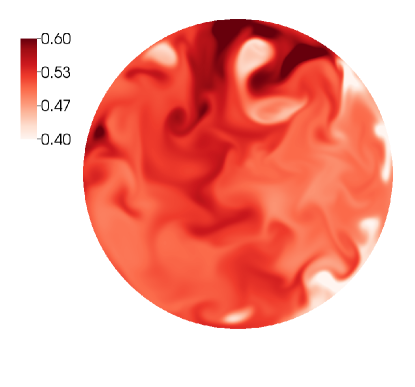
Figure 2: (Colour online) Snapshots of horizontal cross sections at mid-plane of temperature field (left) and velocity magnitude (right) for $Ra=10^{8}$ and $Pr=0.021$ (top row) and $Pr=0.7$ (bottom row). The data for $Ra=10^{8}$ and $Pr=0.7$ have been taken from Scheel & Schumacher (2014).

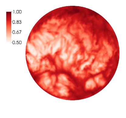
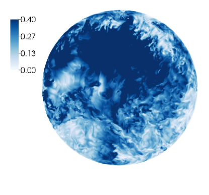
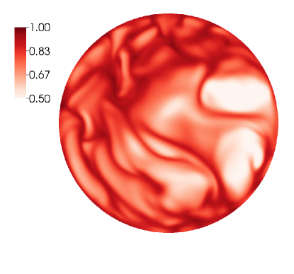
Figure 3: (Colour online) Snapshots of horizontal cross sections at $\delta_{T}/2$ of temperature field (left) and velocity magnitude (right) for $Ra=10^{8}$ and $Pr=0.021$ (top row) and $Pr=0.7$ (bottom row). The data for $Ra=10^{8}$ and $Pr=0.7$ have been taken from Scheel & Schumacher (2014).

A comparison of the instantaneous data for the same Rayleigh number of $Ra=10^{8}$ and $Pr=0.021$ (top row) versus $Pr=0.7$ (bottom row) is shown in figures 2 and 3. Color density plots for both the temperature (left column) and velocity magnitude (right column) are shown for a representative snapshot. A horizontal cut through the cell ($z=1/2$) and inside the thermal boundary layer ($z=\delta_{T}/2$) is shown in figures 2 and 3, respectively. We see in both cases that the temperature is much more diffuse in the lower $Pr$ case, but the velocity is both higher in magnitude and exhibits finer structure and larger fluctuations. This combination of a diffuse temperature field coupled with a stronger fluctuating velocity field give rise to rather different dynamics.

3 Global turbulent heat and momentum transfer

In figure 4 we plot the Nusselt number as a function of Rayleigh number for all three Prandtl numbers (circles for $Pr=0.7$, stars for $Pr=0.021$ and diamonds for $Pr=0.005$). We also added the data for $Pr=6$ which we also have for $Ra=1\times 10^{7}$ (see Scheel et al. (2013)). As expected there is a decrease in heat transport for a given Rayleigh number as Prandtl number decreases. We find the scaling exponent decreases from $0.29\pm 0.01$ to $0.26\pm 0.01$ to $0.265\pm 0.01$ for $Pr=0.7,0.021,0.005$, respectively (see table 2). It should be stressed that the present data base for the low–Prandtl–number simulations is still rather small.

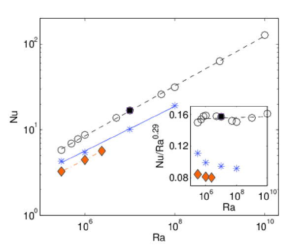
Figure 4: (Colour online) Nusselt number versus Rayleigh number for $Pr=0.005$ (diamonds), $Pr=0.021$ (stars), $Pr=0.7$ (open circles), and $Pr=6$ (filled square). The lines are fits to the data and are given in table 2. The inset replots all data compensated by $Ra^{0.29}$.

Quantity	$Pr=0.7$	$Pr=0.021$	$Pr=0.005$
$Nu$	$(0.15\pm 0.01)Ra^{0.29\pm 0.01}$	$(0.15\pm 0.04)Ra^{0.26\pm 0.01}$	$(0.11\pm 0.02)Ra^{0.265\pm 0.01}$
$Re$	$(0.24\pm 0.01)Ra^{0.49\pm 0.01}$	$(7.4\pm 0.6)Ra^{0.44\pm 0.01}$	$(9\pm 1)Ra^{0.49\pm 0.01}$

Table 2: Fits to the data in figure 4 (for Nusselt number $Nu$ versus Rayleigh number $Ra$) and figure 5 (for Reynolds number $Re$ versus $Ra$). The uncertainty is determined by the scatter in the data and is the result of performing a least squares fit

.

Figure 5: (Colour online) Reynolds number versus Rayleigh number for $Pr=0.005$ (diamonds), $Pr=0.021$ (stars) and $Pr=0.7$ (open circles). The lines are fits to the data and are given in table 2. The inset replots all data compensated by $Ra^{0.49}$.

Figure 6: (Colour online) Nusselt number versus Prandtl number for three different Rayleigh numbers which are indicated in the legend. The solid lines are the fit to the Grossmann-Lohse equations as given in Stevens et al. (2013).

The scaling results are compared with previous published results in table 3, where the coefficients are given by

$$Nu=\alpha Ra^{\beta}.$$ (10)

For $Pr=0.021$, our exponent $\beta$ and prefactor $\alpha$ agree within our uncertainty with experiments by Rossby (1969), Cioni et al. (1996), Takeshita et al. (1996), King & Aurnou (2013), and simulations by Kerr & Herring (2000) and Camussi & Verzicco (1998). However, our exponent is on the high end of the range and our prefactor is on the low end of the range in table 3.

To our knowledge, we can compare our results for $Pr=0.005$ to only one other convection experiment in liquid sodium which has been conducted at the Forschungszentrum Karlsruhe by Horanyi et al. (1999) and shown in table 3. Very recent experiments by Frick et al. (2015) have been conducted in cylindrical cells with a very low aspect ratio of $\Gamma=0.2$. Such a geometry will generate a complex large-scale circulation (LSC) pattern that consists of several rolls on top of each other rather than a single roll as for $\Gamma\sim 1$. Therefore, these experiments are not used for comparison. Our Nusselt number value at $Ra=1\times 10^{6}$ is $Nu=4.45$ (see table 1) which is higher than the $Nu\simeq 4.0$ which is reported by Horanyi et al. (1999). But, our data agrees well for both the exponent and prefactor, within our numerical error. The conclusion which we can draw from the limited amount of data sets is that the scaling exponents $\beta$ we find from our DNS decrease as $Pr$ decreases, and agree with experiments and simulations when the uncertainty is taken into account. However, our measured exponents are 5% larger than the 1/4 scaling reported in some experiments (such as King & Aurnou (2013)) and 30% larger than the 1/5 scaling predicted theoretically by Grossmann & Lohse (2000). However, the difficulty of maintaining isothermal boundary conditions for liquid metals as noted in Horanyi et al. (1999), should be taken into consideration for the experiments. It was found numerically by Verzicco & Sreenivasan (2008) that when constant heat flux was used as the plate boundary conditions instead of isothermal, the Nusselt number for the largest Rayleigh numbers was reduced. This was attributed to the inhibition of thermal plume growth with constant heat flux. This could account for the smaller experimentally measured scaling exponents.

Group	$\ \Gamma\$	$Pr$	Range of $Ra$	$\alpha$	$\beta$
Current work*	1	0.021	$3\times 10^{5}-10^{8}$	0.15 $\pm$ 0.04	0.26 $\pm$ 0.01
Rossby (1969)	2	0.025	$2\times 10^{4}-5\times 10^{5}$	0.147	0.257 $\pm$ 0.004
Cioni et al. (1996)	1	0.025	$5\times 10^{6}-5\times 10^{8}$	0.14 $\pm$ 0.005	0.26 $\pm$ 0.02
Camussi & Verzicco (1998)*	1	0.022	$5\times 10^{4}-10^{6}$	—	0.25
Takeshita et al. (1996)	1	0.025	$10^{6}-5\times 10^{8}$	0.155	0.27 $\pm$ 0.02
Glazier et al. (1999)	2,1,0.5	0.025	$2\times 10^{5}-8\times 10^{10}$	—	0.29 $\pm$ 0.01
Kerr & Herring (2000)*	4	0.07	$10^{4}-10^{7}$	—	0.26
King & Aurnou (2013)	1	0.025	$5\times 10^{6}-10^{8}$	0.19	0.249
Current work*	1	0.005	$3\times 10^{5}-2\times 10^{6}$	0.11 $\pm$ 0.02	0.265 $\pm$ 0.01
Horanyi et al. (1999)	4.5	0.006	$2\times 10^{4}-5\times 10^{6}$	0.115	0.25

Table 3: Comparison of scaling coefficients for Nusselt number with Rayleigh number (see equation (10)). We only selected cases which overlapped with our data range. The asterisks indicate numerical simulations; the others are experiments.

We then investigate the dependence of Reynolds number $Re$ on Rayleigh number in figure 5 using equation (8) to compute our Reynolds numbers. We find that the Reynolds number increases rather significantly as Prandtl number decreases, which is a reflection of the much stronger velocity field. The scaling exponent is similar, but has decreased with Prandtl number from $0.49\pm 0.01$ for $Pr=0.7$ to $0.44\pm 0.01$ for $Pr=0.021$, but then returns to $0.49\pm 0.01$ for $Pr=0.005$. Experimentally Takeshita et al. (1996) found $Re=6.24Ra^{0.46\pm 0.02}$ for $Pr=0.025$ which agrees with our exponent and prefactor. In the simulations done by Verzicco & Camussi (1999) a scaling law $Re\simeq Ra^{0.53}$ is found which does not agree with our results.

In figure 6 we show the Nusselt number as a function of Prandtl number for three Rayleigh numbers. Also included as solid lines are fits to the scaling theory by Grossmann & Lohse (2001) with the updated prefactors from Stevens et al. (2013). The fits are very good, especially for $Pr=0.7$ and 6. However we do see a consistent disagreement for the lower Prandtl numbers, with the Grossmann-Lohse theory slightly underestimating the value for the Nusselt number. This was also seen in the simulations by van der Poel et al. (2013).

4 Turbulence statistics for constant Grashof number

In Schumacher et al. (2015), we emphasized that a change in the parameter variation from constant $Ra$ to constant $Gr$ sheds a different light on the Prandtl number dependence in turbulent convection. Studies at constant Grashof number require a simultaneous variation of both the Rayleigh and Prandtl numbers as seen in figure 1. In this case, the momentum equation (3) remains unchanged. The explicit Prandtl number dependence appears only in the advection–diffusion equation (4). There is however an indirect Prandtl number dependence in the momentum equation as well. This is manifest in the buoyancy term. A more diffusive temperature field injects kinetic energy at a larger scale into the convection flow, as demonstrated in Schumacher et al. (2015).

In figures 7 and 8 we compare root-mean-square (rms) profiles for different Prandtl number but fixed Grashof number for runs 1, 4 and 8. The rms values are defined as follows:

$$u_{rms}(z)=\sqrt{\langle u_{i}^{2}\rangle_{A,t}}\,,\;\;\;w_{rms}(z)=\sqrt{\langle u_{z}^{2}\rangle_{A,t}}\,,\;\;\;\theta_{rms}(z)=\sqrt{\langle(T-\langle T\rangle_{A,t})^{2}\rangle_{A,t}}\,.$$ (11)

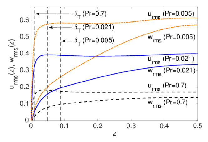
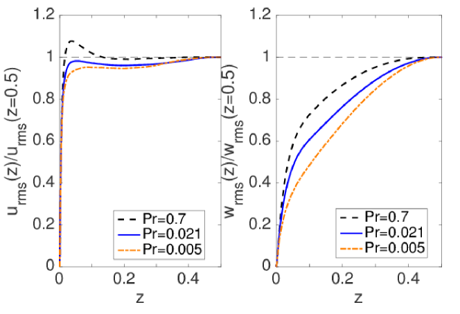
Figure 7: (Colour online) Root-mean-square (rms) velocity profiles for various Prandtl numbers. Upper panel: The total rms velocity, $u_{rms}$, and the vertical rms velocity, $w_{rms}$, are given by equations (11). The thermal boundary layer thicknesses $\delta_{T}$ obtained from (23) are also shown. All profiles are additionally averaged over the lower and upper halves of the cell. Lower left panel: Profiles of $u_{rms}$ collapsed with respect to their amplitude in the midplane. Lower right panel: Profiles of $w_{rms}$ collapsed with respect to their amplitude in the midplane. All data sets are for $Gr=4.76\times 10^{8}$.

The upper panel of figure 7 displays the expected increase of the velocity fluctuations, and thus of the turbulent kinetic energy, with decreasing Prandtl number. The vertical velocity fluctuations, $w_{rms}$ yield a significant contribution to $u_{rms}$ at all heights. As visible in the rescaled plot of lower right panel of figure 7, the profiles of $w_{rms}$ always monotonically increase towards the cell center plane at $z=0.5$. They form an increasingly wider plateau around the center plane when the Prandtl number increases. Furthermore, in the lower left panel of the same figure that for the lowest Prandtl number case, we detect that the maximum of the profiles of $u_{rms}$ is found at $z=0.5$. This is different from the case for $Pr=0.7$ where the fluctuations obey a maximum at $z\approx\delta_{T}$ which can be attributed to the finer thermal plumes which detach from both boundary layers at higher $Pr$.

The profiles of the rms of the temperature fluctuations are shown in the top panel of figure 8. All three profiles obey a local maximum that is close to the thermal boundary layer thickness. The maximum amplitude of the root mean-square-temperature fluctuations is of about the same magnitude for the two larger Prandtl numbers and drops significantly for the smallest accessed Prandtl number of $Pr=0.005$. For the latter case, the temperature field is so diffusive such that a detachment of several separate thermal plumes is not observed anymore. Rather one pronounced hot upwelling on one side of the cell is found in combination with a pronounced cold downwelling on the diametral side. In other words, the LSC is driven by a single pair of plumes which causes the drop in fluctuations.

The bottom panel of figure 8 shows the rescaled mean temperature profiles for the same data in the vicinity of the bottom plate. Following Shishkina & Thess (2009) we define

$$\Theta(y)=2-2\langle T(z)\rangle_{A,t}\quad\text{with}\quad y=2Nu\,z=z/\delta_{T}\,.$$ (12)

The dotted line indicates the slope of one of the profiles close to the wall. We see that the profiles for the low Prandtl numbers start to differ from the one for convection in air further away from the wall. The data for the lowest Prandtl number display an increase of $\Theta$ above one which indicates a positive slope of the unscaled mean temperature profile in the bulk. This behavior is most probably attributed to the small Rayleigh number that was used in the sodium case.

The vertical profiles of the plane-time averages of kinetic energy dissipation and thermal dissipation rate fields are plotted in figure 9. They are denoted by $\varepsilon(z)=\langle\varepsilon\rangle_{A,t}$ and $\varepsilon_{T}(z)=\langle\varepsilon_{T}\rangle_{A,t}$, respectively. The thermal dissipation rate field is given by

$${\varepsilon}_{T}({\bf x},t)=\frac{1}{\sqrt{Gr}\,Pr}\left(\frac{\partial T}{\partial x_{j}}\right)^{2}\,,$$ (13)

and the kinetic energy dissipation rate field is defined as

$$\varepsilon({\bf x},t)=\frac{1}{2\sqrt{Gr}}\left(\frac{\partial u_{i}}{\partial x_{j}}+\frac{\partial u_{j}}{\partial x_{i}}\right)^{2}\,.$$ (14)

The profiles imply that both dissipation rates increase in magnitude as the Prandtl number decreases. While the thermal dissipation rate grows as a result of the enhanced thermal diffusivity, the kinetic energy dissipation is increased as a result of the enhanced small-scale intermittency. The latter result has to be a consequence of enhanced local velocity derivatives since the prefactor in (14) is unchanged. The ratios $Q_{T}=\varepsilon_{T}(z=0)/\varepsilon_{T}(z=0.5)$ and $Q_{v}=\varepsilon(z=0)/\varepsilon(z=0.5)$ give $Q_{T}\simeq 840,100,60$ and $Q_{v}\simeq 19,16,19$, respectively, for Prandtl numbers $Pr=0.7,0.021,0.005$. While the ratio of kinetic energy dissipation between boundary layer and bulk remains more or less unchanged, the dominance of thermal dissipation in the boundary layers for large Prandtl numbers is significantly diminished.

The local enstrophy can be defined by means of the vorticity field $\omega_{i}=\epsilon_{ijk}\partial_{j}u_{k}$ with $i,j,k=1,2,3$ and is given by

$$\Omega({\bf x},t)=\omega_{i}({\bf x},t)\omega_{i}({\bf x},t)\,.$$ (15)

In homogeneous isotropic turbulence the ensemble averages of the mean dissipation and the local enstrophy are connected by an exact relation which translates in our units into

$$\langle\varepsilon\rangle=\frac{1}{\sqrt{Gr}}\langle\Omega\rangle\,.$$ (16)

Figure 10 shows that this relation is satisfied to a good approximation even in our closed cylindrical cell when we compare the vertical mean profiles $\epsilon(z)$ and $\Omega(z)/\sqrt{Gr}$. The dashed lines for the energy dissipation rate and the corresponding solid lines for the rescaled local enstrophy are found to collapse almost perfectly.

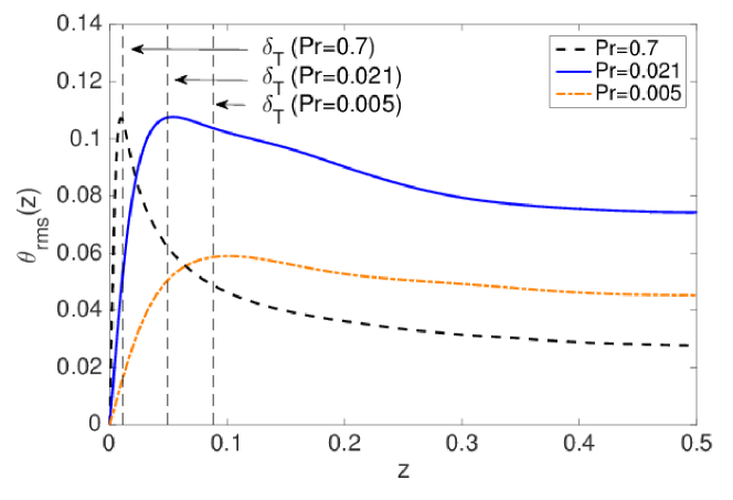
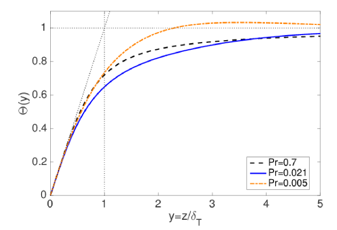
Figure 8: (Colour online) Temperature field statistics for various Prandtl numbers. Top: The time averaged temperature deviation $\theta_{rms}$ is given by equation (11). The thermal boundary layer thicknesses $\delta_{T}$ obtained from (23) are also shown. All profiles are additionally averaged over the lower and upper halves of the cell. Bottom: Scaled mean temperature profiles $\Theta(y)$ versus $y=z/\delta_{T}$ (see equation (12)). All data sets are for $Gr=4.76\times 10^{8}$.

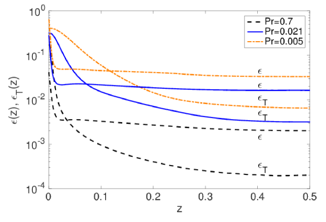
Figure 9: (Colour online) Energy dissipation rate profiles for various Prandtl numbers. The kinetic energy dissipation rate $\epsilon$ and thermal dissipation rate $\epsilon_{T}$ are given by area–time averages of equations (14) and (13), respectively. All profiles are additionally averaged over the lower and upper halves of the cell. All data sets are for $Gr=4.76\times 10^{8}$.

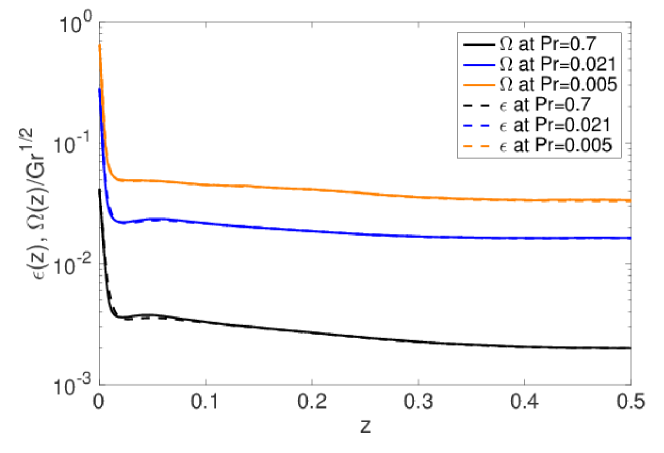
Figure 10: (Colour online) Mean kinetic energy dissipation rate and rescaled local enstrophy profiles for various Prandtl numbers. All profiles are additionally averaged over the lower and upper halves of the cell. All data sets are for $Gr=4.76\times 10^{8}$.

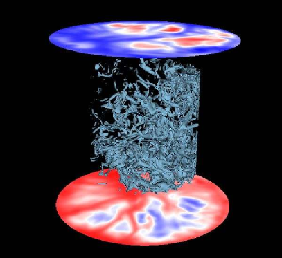
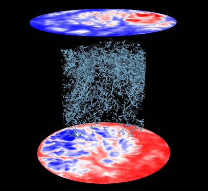
Figure 11: (Colour online) Isosurfaces of constant enstrophy for $Pr=0.021$. Left panel: $Ra=10^{7}$, and $1\times 10^{4}<\Omega<1\times 10^{5}$. Right panel: $Ra=10^{8}$ and $3.5\times 10^{4}<\Omega<5\times 10^{4}$. Also shown are the temperature field at cuts through the bottom and top boundary layers. (Movie available online.)

5 Local statistical analysis

Isosurfaces of the local enstrophy are plotted in figure 11 for $Pr=0.021$ for two different Rayleigh numbers, along with plots of the temperature field at two horizontal cross sections in the thermal boundary layers. The plot, which excludes the field at the side walls, displays the fine structure of the characteristic vortex tubes, which are well-known from homogeneous isotropic turbulence (Kerr (1985)). Enhanced small-scale intermittency was found to be in line with ever finer vortex tubes as discussed by Ishihara et al. (2009). This is exactly what we detect in the center of the convection cell when comparing the two isosurface plots. In the following we want to investigate in detail if this enhanced intermittency in the bulk is in line with enhanced intermittency in the boundary layers, in particular in the velocity boundary layer.

5.1 Skin friction scaling

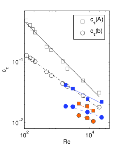
Figure 12: (Colour online) Comparing friction coefficient $c_{\tau}(A)$ as defined in Eq. (22) versus Rayleigh number in the left panel and versus Reynolds number in the right panel, for $Pr=0.005$ (filled circles with black outline), $Pr=0.021$ (filled circles) and $Pr=0.7$ (open circles). Also plotted is $c_{\tau}(b)$ as defined in Eq. (22) versus Rayleigh number (or Reynolds number) for $Pr=0.005$ (filled squares with black outline), $Pr=0.021$ (filled squares) and $Pr=0.7$ (open squares). The lines are fits to the data and are given in table 4.

We start with the definition of the skin-friction coefficient (see e.g. Schlichting & Gersten (2000)) which is defined as

$$c_{\tau}=\frac{\langle\hat{\tau}_{w}\rangle}{\hat{\rho}_{0}\hat{U}^{2}/2}\,,$$ (17)

where $\langle\cdot\rangle$ is an ensemble average. The coefficient relates the mean wall shear stress to the dynamic pressure. The hat indicates a quantity with dimension. Here, $\hat{\rho}_{0}$ is the constant mass density of the fluid and $\hat{U}$ a characteristic velocity which will be specified further below. The following definition of the wall shear stress field at the plate is used

$$\hat{\tau}_{w}(\hat{x},\hat{y},\hat{z}=0,\hat{t})=\hat{\rho}_{0}\hat{\nu}\sqrt{\Bigg{|}\frac{\partial{\hat{u}_{x}}}{\partial\hat{z}}\Bigg{|}_{\hat{z}=0}^{2}+\Bigg{|}\frac{\partial{\hat{u}_{y}}}{\partial\hat{z}}\Bigg{|}_{\hat{z}=0}^{2}}\,.$$ (18)

Following Scheel & Schumacher (2014) this can be related to a local thickness of the velocity boundary layer by

$$\hat{\lambda}_{v}^{o}(\hat{x},\hat{y},\hat{z}=0,\hat{t})=\frac{\hat{\rho}_{0}\hat{\nu}\hat{u}_{rms,V}}{\hat{\tau}_{w}(\hat{x},\hat{y},\hat{z}=0,\hat{t})}\,,$$ (19)

excluding zero-stress events. If we assume that the $\hat{U}$ in (17) is also given by $\hat{u}_{rms,V}$ (see equation (8)) and express all variables in units of $H,U_{f}$ and $\Delta T$ (see section 2), we obtain the following definition for $c_{\tau}$

$${c_{\tau}}=\frac{2}{Re\langle\lambda_{v}^{o}\rangle}\,,$$ (20)

where $Re$ is defined in (8) and the mean outer velocity boundary layer thickness is found by

$$\langle\lambda^{o}_{v}\rangle=\int_{0}^{\infty}\,\lambda^{o}_{v}\,p(\lambda^{o}_{v})\,\mbox{d}\lambda^{o}_{v}\,,$$ (21)

with $p(\lambda^{o}_{v})$ being the probability density function (PDF) of the outer velocity boundary layer thickness.

Rather than an ensemble average, a plane-time average is performed. Averages over the entire plate area $r\leq 0.5$ will denoted by $\langle\cdot\rangle_{A,t}$ or over the interior plate area $r_{c}<0.3$ by $\langle\cdot\rangle_{b,t}$. Thus the two friction coefficients are given as

$${c_{\tau}}(A)=\frac{2}{Re\langle\lambda_{v}^{o}\rangle_{A,t}}\quad\text{and}\quad{c_{\tau}}(b)=\frac{2}{Re\langle\lambda_{v}^{o}\rangle_{b,t}}\,,$$ (22)

For the interior average, we selected a range of cutoff radii from $0.2<r_{c}<0.4$ and found that the results for scaling exponents and prefactors do not change significantly. However, there is a systematic trend towards smaller boundary layer thicknesses (and hence larger values of $c_{\tau}(b)$) as $r_{c}$ decreases. We chose $r_{c}=0.3$ as our cutoff radii for all plots. The uncertainty in the values in table 4 for interior averages is based on how the results vary as $r_{c}$ varies. In other words, the scaling exponent was found for $0.2<r_{c}<0.4$ and the difference between the largest and smallest scaling exponent is given as the uncertainty in scaling exponent. Likewise for the prefactor.

We have plotted $c_{\tau}$ as a function of Rayleigh number and Reynolds number for $Pr=0.005,0.021,0.7$, and also compare the whole area and the interior averages in figure 12. The resulting power law fits are given in table 4. In all cases the skin friction magnitude and scaling exponent are reduced when the side-wall regions are included. For the scaling with respect to the Reynolds number equation (8) is used.

Which scaling exponents can be expected for a velocity boundary layer in turbulent convection in the present Rayleigh number range? One limiting case for the skin-friction coefficient could be that of a laminar, stationary, two-dimensional, zero-pressure gradient flat plate boundary layer (Blasius (1908)). There $c_{f}\sim Re_{L}^{-1/2}$ with $Re_{L}$ being the Reynolds number which is composed of the constant outer inflow velocity $\hat{U}_{\infty}$ and the downstream length $\hat{L}$ of the flat plate. The other limiting case for our present flow could be that of a fully developed turbulent flat plate boundary layer which yields a scaling law of the skin-friction coefficient which can be approximated by $c_{f}\sim Re_{L}^{-1/5}$ for $5\times 10^{5}\lesssim Re_{L}\lesssim 10^{7}$ (Coles & Hirst (1969)).

Clearly, these limiting cases neglect buoyancy effects which are present in the RBC flow. Furthermore, the flat plate Reynolds number $Re_{L}$ cannot be directly associated with the present $Re$. We see that for the $Pr=0.7$ case, the scaling exponent for $c_{f}$ taken for $A$ is a bit smaller than the laminar limit. When the side-wall regions at the plate are excluded and the average is taken over $b$, the scaling exponent is found to be very close to the laminar limit. For the lower Prandtl numbers, the scaling with Reynolds number when the side-wall regions are included agrees within the error bars with the exponent of -0.2 for a turbulent boundary layer although the Reynolds numbers are by more than an order of magnitude smaller than $Re_{L}$. When the side walls are excluded, the scaling with Reynolds number is found to take values around -0.25. Not only does the bulk of the convection flow display more vigorous turbulence as $Pr$ decreases, but the same seems to hold for the velocity boundary layer as the global scaling of the skin-friction coefficient suggests.

5.2 Boundary layer thickness scaling

We can define boundary layer thicknesses in terms of the global heat and momentum transfer (see Grossmann & Lohse (2000)) by

$$\hat{\delta}_{T}=\frac{\hat{H}}{2Nu}\,,$$ (23)

and

$$\hat{\delta}_{v}=\frac{a\hat{H}}{\sqrt{Re}}\,.$$ (24)

Note that $a$ is a free parameter (Prandtl 1905, Blasius 1908) which is set to $a=1/4$ in the present case following Grossmann & Lohse (2001). We define the (dimensionless) mean thermal boundary layer thicknesses by Scheel & Schumacher (2014) to be

$$\lambda_{T}^{o}=\frac{1}{2}\Bigg{|}\frac{\partial{T}}{\partial{z}}\Bigg{|}_{z=0}^{-1},\qquad\langle\lambda^{o}_{T}\rangle=\int_{0}^{\infty}\,\lambda^{o}_{T}\,p(\lambda^{o}_{T})\,\mbox{d}\lambda^{o}_{T}.$$ (25)

Figure 13 summarizes our findings for the series of low–$Pr$ runs and compares them with the data obtained by Scheel & Schumacher (2014). The scaling exponents for convection in air agree to a good approximation with those for liquid-metal convection, but with slightly decreasing exponent magnitude as $Pr$ decreases, which is consistent with the scaling for $Nu(Ra)$. The value for $\langle\lambda_{T}\rangle$ is always larger for the low–$Pr$ case. The boundary layer thickness is also larger when the side-wall regions are included. It is observed that this difference is consistently larger for the low–$Pr$ case, even with increasing $Ra$. The plumes that detach from the plates are coarser due to enhanced thermal diffusion and cause larger variations in the local boundary layer thickness.

Figure 13: (Colour online) Left panel: Scaling of mean thermal boundary layer thickness with Rayleigh number for different analysis methods and different Prandtl number. The filled data points with black outlines are for $Pr=0.005$, The filled data points are for $Pr=0.021$ and the open symbols are for $Pr=0.7$. The squares for $\langle\lambda_{T}^{o}\rangle_{A}$ are taken over the whole plate area, the diamonds are for $\langle\lambda_{T}^{o}\rangle_{b}$ taken over the interior area with $r<0.3$. Circles correspond to the theoretical values for $\delta_{T}=1/(2Nu)$. All data are also averaged with respect to time. The fits are given in table 4. Right panel: the same data sets replotted where all the mean thermal boundary layer thickness data (represented by “$\lambda_{T}$”) are compensated by $Ra^{-0.29}$.

Quantity	$Pr=0.7$	$Pr=0.021$	$Pr=0.005$
$c_{\tau}(A)$	$(1.4\pm 0.1)Ra^{-0.19\pm 0.01}$	$(0.05\pm 0.01)Ra^{-0.08\pm 0.01}$	$(0.05\pm 0.01)Ra^{-0.11\pm 0.02}$
	$(0.79\pm 0.05)Re^{-0.39\pm 0.01}$	$(0.07\pm 0.01)Re^{-0.17\pm 0.02}$	$(0.80\pm 0.03)Re^{-0.22\pm 0.03}$
$c_{\tau}(b)$	$(12\pm 2)Ra^{-0.27\pm 0.01}$	$(0.18\pm 0.10)Ra^{-0.12\pm 0.03}$	$(0.08\pm 0.03)Ra^{-0.11\pm 0.03}$
	$(5.7\pm 0.7)Re^{-0.54\pm 0.01}$	$(0.31\pm 0.1)Re^{-0.27\pm 0.02}$	$(0.14\pm 0.08)Re^{-0.23\pm 0.04}$
$\langle\lambda_{T}^{o}\rangle_{A}$	$(5.9\pm 0.2)Ra^{-0.31\pm 0.01}$	$(5\pm 2)Ra^{-0.26\pm 0.01}$	$(3.8\pm 0.5)Ra^{-0.22\pm 0.01}$
$\langle\lambda_{T}^{o}\rangle_{b}$	$(2.3\pm 0.3)Ra^{-0.26\pm 0.01}$	$(3\pm 2)Ra^{-0.25\pm 0.02}$	$(4.0\pm 1)Ra^{-0.25\pm 0.01}$
$\delta_{T}$	$(3.3\pm 0.3)Ra^{-0.29\pm 0.01}$	$(3\pm 1)Ra^{-0.26\pm 0.01}$	$(4.4\pm 0.5)Ra^{-0.26\pm 0.01}$
$\langle\lambda_{v}^{o}\rangle_{A}$	$(5.9\pm 0.7)Ra^{-0.30\pm 0.01}$	$(5.4\pm 1)Ra^{-0.36\pm 0.01}$	$(4\pm 1)Ra^{-0.38\pm 0.01}$
$\langle\lambda_{v}^{o}\rangle_{b}$	$(0.55\pm 0.18)Ra^{-0.21\pm 0.01}$	$(1.5\pm 1)Ra^{-0.32\pm 0.02}$	$(2.5\pm 1)Ra^{-0.38\pm 0.03}$
$\delta_{v}$	$(0.50\pm 0.02)Ra^{-0.25\pm 0.01}$	$(0.094\pm 0.003)Ra^{-0.22\pm 0.01}$	$(0.082\pm 0.004)Ra^{-0.25\pm 0.01}$

Table 4: Fits to the data in figure 12 for friction coefficient $c_{\tau}$ versus Rayleigh number $Ra$ averaged over the entire plate area ($A$) or over only the interior ($b$), $r<0.3$. Also given are fits to the data in figures 13 and 14 for local boundary layer thickness versus $Ra$ averaged over time and the entire plate area ($\langle\lambda_{T}^{o}\rangle_{A}$, and $\langle\lambda_{v}^{o}\rangle_{A}$) or over only the interior plate area ($\langle\lambda_{T}^{o}\rangle_{b}$ and $\langle\lambda_{v}^{o}\rangle_{b}$). Also fit are the boundary layer thicknesses $\delta_{T}$ obtained from Nusselt number and $\delta_{v}$ obtained from the Reynolds number. The uncertainty for all area averaged quantities and $\delta_{T}$, $\delta_{v}$ is determined by the scatter in the data and is the result of performing a least squares fit. The uncertainty in the interior averages is discussed just after (22).

Figure 14 summarizes our findings for $\langle\lambda_{v}^{o}\rangle$, which is defined in (21). We find that $\langle\lambda_{v}^{o}\rangle$ is significantly smaller for the low–$Pr$ case. We also find that the scaling exponent for $\langle\lambda_{v}^{o}\rangle$ for the low–$Pr$ cases becomes larger in magnitude as $Pr$ decreases. Since $\langle\lambda_{v}^{o}\rangle$ is determined from the inverse of the velocity gradients, this suggests that the magnitudes of these gradients get larger with $Ra$ at a faster rate for the lower $Pr$ case. However, the scaling exponent for $\delta_{v}$ as measured from the Reynolds number for $Pr=0.021$ case is a bit smaller in magnitude than that for convection in air ($Pr=0.7$) or liquid sodium ($Pr=0.005$), consistent with our results from figure 5.

Figure 14: (Colour online) Scaling of mean velocity boundary layer thickness with Rayleigh number for different analysis methods and different $Pr$. The filled data points with black outlines are for $Pr=0.005$, the filled data points are for $Pr=0.021$, and the open symbols are for $Pr=0.7$. The squares are for $\langle\lambda_{v}^{o}\rangle_{A}$ taken over the whole cell and the diamonds are for $\langle\lambda_{v}^{o}\rangle_{b}$ taken over the interior plate area. The circles are the theoretical values for $\delta_{v}=a/\sqrt{Re}$ with the Reynolds numbers taken from table 1 and $a=1/4$. All data is averaged with respect to time. The fits are again listed in table 4.

5.3 Local shear Reynolds number

We define the local shear Reynolds number as

$$Re_{sh}(x,y)=\sqrt{\frac{Ra}{Pr}}\lambda_{v}^{o}(x,y)u_{rms}(z=\lambda_{v}^{o}(x,y))\,.$$ (26)

This is a good measure of the stability of the flow in the boundary layer. It is similar to equation (41.1) in Landau & Lifshitz (1987) but we pick $u_{rms}$ at $\lambda_{v}^{o}$ because the boundary layer thickness varies locally (see Scheel & Schumacher (2014)), hence it is more straightforward than selecting $U$, the fluid velocity outside the space- and time-averaged boundary layer.

According to Landau & Lifshitz (1987) and Tollmien (1929), when the value of $Re_{sh}\simeq 420$ is exceeded, then the boundary layer is turbulent. The boundary-layer scale that was used for this estimate is the displacement thickness scale, and this applies to two-dimensional turbulent shear flow. We could compute the area and time averaged $Re_{sh}$ to assess when the boundary layer becomes turbulent, which was done in Scheel & Schumacher (2014) and Wagner at al. (2012). But, since the locally calculated $Re_{sh}$ (26) varies strongly and reaches values greater than 420 for local regions of the plate and for large enough Rayleigh number, we can also assess this spatial intermittency by finding the fractional area which is defined as

$${\cal T}=\frac{A({Re_{sh}>Re_{sh}^{c}})}{A}\,,$$ (27)

where the numerator of (27) describes the area of the plate where $Re_{sh}(x,y,t)>Re_{sh}^{c}$, and $Re_{sh}^{c}$ is a critical-shear-threshhold Reynolds number, i.e., 420 in the case of Landau & Lifshitz (1987). We can compute ${\cal T}$ very precisely with the code and our area average uses the local volume element for our collocation data points. Also note that the total area $A$ is given by $\pi/4$.

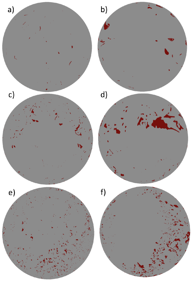
Figure 15: Threshhold plots demonstrating the area of the bottom plate whose shear Reynolds number as calculated in (26) is greater than 250 (red). The gray area denotes shear Reynolds numbers less than 250. The left column is for $Pr=0.7$ and (a) $Ra=1\times 10^{8}$ (c) $Ra=1\times 10^{9}$, and (e) $Ra=1\times 10^{10}$ and the right column is for $Pr=0.021$ and (b) $Ra=1\times 10^{6}$, (d) $Ra=1\times 10^{7}$. (f) $Ra=1\times 10^{8}$.

Since there is no theoretical value for the transition to turbulence in the boundary layer for Rayleigh-Bénard convection, we take three values for $Re_{sh}^{c}:250,350,450$. This brackets a range of possible turbulent onset values (including the value of 420 from Landau & Lifshitz (1987)) and provides calculation of the uncertainty. We plot snapshots of ${\cal T}$ for various Rayleigh and Prandtl numbers in figure 15 to highlight the intermittency. We chose $Re_{sh}>250$ as our cutoff in the figures as this provides a larger region for ${\cal T}$. We see in figure 15 that the structures where $Re_{sh}>250$ are much finer for the higher $Pr$ case and increase more in number as $Ra$ increases.

In figure 16 we look at the time evolution of the fractional area, and note that it varies by about 25%, as is expected for the intermittency in the boundary layer. We also see variation between the top and bottom plate, with some anticorrelation which we attribute to the large-scale circulation. If, for example a plume is ejected from the bottom plate, causing a large value of ${\cal T}$ on the bottom plate, it takes some time for this plume to be swept up to the top plate by the large-scale circulation. Eventually this plume hits the top plate which could cause another plume to be ejected by the top plate, causing ${\cal T}$ to now be larger at the top plate. However, the anticorrelation is not perfect and the situation is more complex, since plume ejection occurs intermittently.

Finally we plot the time averaged ${\cal T}$ in figure 17 and see that the turbulent fraction increases as a function of Rayleigh number for all Prandtl numbers, with the turbulent fraction always being larger for the lower Prandtl number.

In figure 17 we also can determine the critical Rayleigh number $Ra_{Ac}$ where $\langle{\cal T}\rangle_{t}=1$ for our Prandtl numbers and $Re_{sh}^{c}$ values, which would indicate a transition to a fully turbulent boundary layer. We find, using $Re_{sh}^{c}$=350 as our mid-range value, and $Re_{sh}^{c}$=250, 450 as upper and lower bounds, that $Ra_{Ac}=(3\pm 2)\times 10^{13}$ for $Pr=0.7$, $Ra_{Ac}=(2\pm 10)\times 10^{13}$ for $Pr=0.021$. We did not fit the data or estimate an $R_{Ac}$ for $Pr=0.005$ since the data covers an interval which is too small and the Rayleigh numbers are too low for a reasonable extrapolation.

The uncertainty is high in these predicted critical Rayleigh numbers, since we are using data at Rayleigh numbers that are three orders of magnitude smaller than the predicted transition values. However, the critical Rayleigh number for $Pr=0.7$ is close to the value of $Ra_{1}^{*}\simeq 2\times 10^{13}$ found by He et al. (2012); Ahlers et al. (2012) for similar parameters. In these papers the authors noted tha $Ra_{1}^{*}$ indicated a transition from the classical laminar scaling of Nusselt number with Rayleigh number, but the fully turbulent scaling of Nusselt number with Rayleigh number was not seen until $Ra_{2}^{*}\geq 5\times 10^{14}$.

Even though $\langle{\cal T}\rangle_{t}$ increases as $Pr$ decreases, we still find $Ra_{Ac}$ occurs at about the same Rayleigh number for $Pr=0.021$, when the uncertainty is taken into account. This is because the growth of $\langle{\cal T}\rangle_{t}$ with Rayleigh number is so much smaller for the lower $Pr$. The theoretically predicted trend by Grossmann & Lohse (2000) is for $Ra_{Ac}$ to decrease as $Pr$ decreases, and the values as estimated from figure 2 of Grossmann & Lohse (2000) are around $10^{13},10^{14},10^{16}$ for $Pr=0.005,0.021,0.7$, respectively. This disagreement may be due to the higher uncertainty in these data points, or it may be indicative of something more fundamental, i.e. that the transition from a laminar to a turbulent boundary layer may be more universal than previously predicted. However, more data at higher Rayleigh numbers would provide a more precise value for $Ra_{Ac}$.

Figure 16: (Colour online) Time dependence of fractional area ${\cal T}$ (defined in (27) greater than 250 (black line=top plate, magenta (light gray) line=bottom plate). The fractional area is given for each statistically independent snapshot. (a) $Pr=0.7$ and $Ra=1\times 10^{9}$. (b) $Pr=0.021$ and $Ra=1\times 10^{7}$.

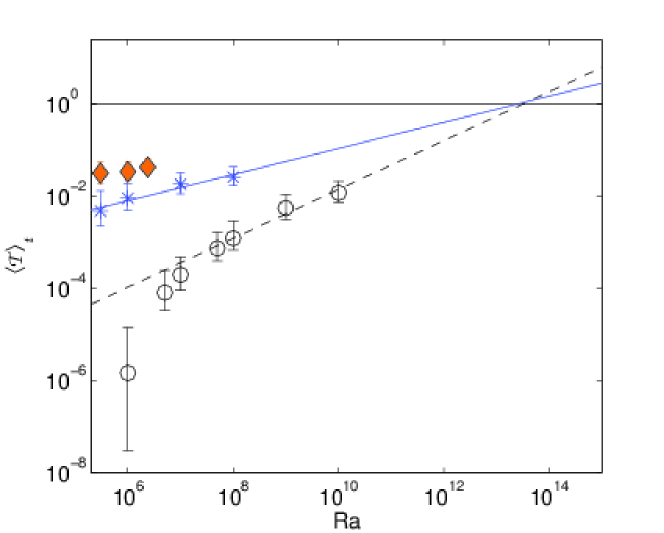
Figure 17: (Colour online) Time averaged turbulent fraction $\langle{\cal T}\rangle_{t}$ of top and bottom plate area whose shear Reynolds number defined in (26) is greater than 350 (black circles, $Pr=0.7$, magenta stars, $Pr=0.021$, yellow filled diamonds with black outline, $Pr=0.005$). The error bars correspond to the cases where $Re_{sh}^{c}=250$ (upper) and $Re_{sh}^{c}=450$ (lower). Note this fraction has been averaged over many statistically independent time slices. The thick black line corresponds to ${\cal T}=1$. The fit to the last four data points for $Pr=0.7$ is $\langle{\cal T}\rangle_{t}=(7\pm 1\times 10^{-7})Ra^{0.5\pm 0.1}$ (dashed line). The fit to all data points for $Pr=0.021$, is $\langle{\cal T}\rangle_{t}=(1.6\pm 1\times 10^{-4})Ra^{0.28\pm 0.05}$ (solid line).

Figure 18: (Colour online) Kurtosis (28) versus Rayleigh number for $Pr=0.7$ (circles), $Pr=0.021$ (stars) and $Pr=0.005$ (diamonds).

We can also check for intermittency by evaluating the kurtosis, as defined in equation (28). For a Gaussian distribution the kurtosis should be equal to three. Anything larger than this indicates wider tails to the distribution, and hence intermittency. The kurtosis is plotted in figure 18 for all Rayleigh and Prandtl numbers. We see that the kurtosis is much larger than three for all data. For $Pr=0.7$, the kurtosis stays fairly level at 500 until $Ra=1\times 10^{8}$ and then it increases with $Ra$. However, for the lower $Pr$ data the kurtosis increases with $Ra$ for all data and the kurtosis values are also very close to one another.

$$\mbox{Kurtosis}=\dfrac{\langle(Re_{sh}-\langle Re_{sh}\rangle)^{4}\rangle}{\langle(Re_{sh}-\langle Re_{sh}\rangle)^{2}\rangle^{2}}$$ (28)

6 Summary and discussion

A comparison of the global and local statistics has been presented for low $Pr$ numbers ($Pr=0.005,0.021$) and those of air ($Pr=0.7$) with very finely-resolved DNS. The low $Pr$ cases are in a parameter regime that has not been studied numerically at such fine resolution. It is found that the temperature field is more diffuse while the velocity field is more vigorous as the Prandtl number is lowered. It is also found that as the Prandtl number decreases there is a slight overall decrease in the value of the scaling exponents of diagnostic quantities, such as Nusselt number and thermal boundary layer thicknesses, with Rayleigh number. We attribute this to the more diffuse temperature field and resulting reduced heat transport as $Pr$ decreases to these very low values.

The global heat transfer scaling exponents are found to have values of $0.29\pm 0.01$, $0.26\pm 0.01$ and $0.265\pm 0.01$ for $Pr=0.7,0.021$ and $0.005$ respectively. When compared with experimental results of Horanyi et al. (1999), the present exponents are found to agree quite well for $Pr=0.005$. The exponent for $Pr=0.021$ agrees with the experiments by Rossby (1969), Cioni et al. (1996), Takeshita et al. (1996), King & Aurnou (2013). However our exponent is on the high end of the range, and disagrees with the theory which predicts a scaling exponent of 1/5 for this parameter regime in Grossmann & Lohse (2000). The global momentum scaling exponents are $0.49\pm 0.01,0.44\pm 0.01,0.49\pm 0.01$ for $Pr=0.7,0.021,0.005$. For the case of $Pr=0.021$, they agree well with the experimental results by Takeshita et al. (1996). Finally it is found that when the Nusselt number is plotted versus Prandtl number, the agreement with the Grossmann-Lohse theory is quite good, except for a slight disagreement in the lower Prandtl numbers ($0.021,0.005$). It is stressed once more that the number of data points of our DNS is small and that the predictions of the scaling exponents for global heat and mass transfer should be considered with caution.

The root-mean-square profiles of velocity show a significant enhancement of velocity with decreasing $Pr$ and a shift of the maxima towards the center of the container. The root-mean-square profiles of temperature show similar values for the location of the maxima for $Pr=0.7,0.021,0.005$, but a reduction in overall root-mean-square temperature for $Pr=0.005$. Finally we see that the magnitude of the vertical mean profiles of $\epsilon$ and $\epsilon_{T}$ systematically increases as $Pr$ decreases as is expected. The kinetic dissipation rate increases due to the enhanced velocity fluctuations and the thermal dissipation rate increases due to the higher diffusivity of the temperature field. The agreement between profiles of $\epsilon(z)$ and $\Omega(z)/\sqrt{Gr}$ are also very good, similar to that found for homogeneous isotropic turbulence.

When we compute the thermal boundary layer thicknesses we find that they are also consistently larger as $Pr$ decreases, as expected. Also the magnitude of the scaling exponents decrease slightly as $Pr$ decreases, consistent with the $Nu$ scaling. In contrast, the velocity boundary layer thicknesses are consistently smaller as $Pr$ decreases and the scaling exponent magnitudes increase as $Pr$ decreases. The effect of the side walls is found to remain significant for the lower $Pr$ cases ($0.021$ and $0.005$) as Rayleigh number increases but it becomes less significant for $Pr=0.7$.

Turning now to the local statistics, it is found that the skin-friction coefficient $c_{\tau}$ is significantly reduced as $Pr$ decreases for all Rayleigh numbers, averaging either over the central region or the whole plate. It is also found that the scaling exponent with Reynolds number when the side-wall regions are included increases from $-0.54\pm 0.01$ for $Pr=0.7$ (consistent with a laminar boundary layer) to $-0.23\pm 0.04$ for the lowest $Pr$ which bears a closer resemblance to an intermittently turbulent boundary layer. Inspired by this, we compute a local shear Reynolds number and resulting turbulent fraction $\langle{\cal T}\rangle_{t}$. We find that this turbulent fraction increases with Rayleigh number and is larger for the lower Prandtl numbers. By extrapolating to $\langle{\cal T}\rangle_{t}=1$ we can predict the Rayleigh number $Ra_{Ac}$ at which the boundary layer would become fully turbulent. We find $Ra_{Ac}=(3\pm 2)\times 10^{13}$ for $Pr=0.7$ and $Ra_{Ac}=(2\pm 10)\times 10^{13}$ for $Pr=0.021$. It is stressed once more that our prediction is based on an extrapolation which might be wrong once the gap to the high Rayleigh numbers is filled with further DNS data points.

The present analysis has confirmed the results of Schumacher et al. (2015), namely that the fluid turbulence in low-$Pr$ convection is much more strongly driven and reaches a more vigorous turbulence level than comparable convection flows in air or water. The reason for this observation is that the bottleneck in the RBC system – the thermal boundary layer – is thicker due to enhanced diffusion. Coarser thermal plumes can inject kinetic energy at a larger scale as shown in Schumacher et al. (2015) and extend the Kolmogorov-like cascade range in the bulk. This is in line with an enhanced energy flux in the inertial range and a smaller Kolmogorov length. Coarser plumes intensify also the large-scale circulation in the cell and thus amplify the transient and intermittent behavior in the velocity boundary layer which was shown here, e.g. by the skin friction or the local shear Reynolds number. Our current studies indicate that low Prandtl number convection at the same Grashof number may be more susceptible to a transition to turbulence in the tiny boundary layer when compared with convection in air.

Given the very low-$Pr$ data records, a next step would be to refine the analysis in the transient boundary layers and to develop alternative measures that quantify the increasing number of turbulent patches in the velocity boundary layer. These studies are currently under way and will be reported elsewhere.

Helpful discussions with Jonathan Aurnou, Ronald du Puits, Peter Frick and Bruno Eckhardt are acknowledged. The work is supported by Research Unit 1182 and the Research Training Group 1567 of the Deutsche Forschungsgemeinschaft. We acknowledge supercomputing time at the Blue Gene/Q JUQUEEN at the Jülich Supercomputing Centre which was provided by grant HIL09 of the John von Neumann Institute for Computing. Furthermore, we acknowledge an award of computer time provided by the INCITE program. This research used resources of the ALCF at ANL, which is supported by the DOE under contract DE-AC02-06CH11357.

References

- Ahlers et al. (2012) Ahlers, G., He, X., Funfschilling, D., & Bodenschatz, E. 2012 Heat transport by turbulent Rayleigh-Bénard convection for 0.8 and : aspect ratio . New J. Phys. 14, 103012 (39 pages).
- Aurnou & Olson (2001) Aurnou, J. M. & Olson, P. L. 2001 Experiments on Rayleigh–Bénard convection, magnetoconvection and rotating magnetoconvection in liquid gallium. J. Fluid Mech. 430, 283–307.
- Blasius (1908) Blasius, H. 1908 Grenzschichten in Flüssigkeiten mit kleiner Reibung. Z. Math. Physik 56, 1–37.
- Breuer et al. (2004) Breuer, M., Wessling, S., Schmalzl, J. & Hansen, U. 2004 Effect of inertia in Rayleigh-Bénard convection. Phys, Rev. E 69, 026302 (10 pages).
- Camussi & Verzicco (1998) Camussi, R. & Verzicco, R. 1998 Convective turbulence in mercury: Scaling laws and spectra. Phys. of Fluids, 10, 516–527.
- Chillà & Schumacher (2012) F. Chillà and J. Schumacher 2012 New perspectives in turbulent Rayleigh-Bénard convection. Eur. Phys. J. E, 35, 58 (25 pages).
- Cioni et al. (1996) Cioni, S. Ciliberto, S. & Sommeria, J. 1996 Experimental study of high-Rayleigh-number convection in mercury and water. Dyn. Atmos. Ocean, 24, 117–127.
- Cioni et al. (1997) Cioni, S. Ciliberto, S. & Sommeria, J. 1997 Strongly turbulent Rayleigh-Bénard convection in mercury: comparison with results at moderate Prandtl number. J. Fluid Mech., 335, 111–140.
- Cioni et al. (1997a) Cioni, S., Horanyi, S., Krebs, L. & Müller, U. 1997 Temperature fluctuation properties in sodium convection. Phys. Rev. E 56, R3753–R3756.
- Coles & Hirst (1969) Coles, D. E. & Hirst, E. A. 1969 Computation of turbulent boundary layers. Proc. of AFOSR-IFP-Stanford Conference, Vol. II, Stanford University, CA, 1968.
- Deville et al. (2002) Deville, M. O., Fischer, P. F. & Mund, E. H. 2002 High-order methods for incompressible fluid flow Cambridge University Press.
- Glazier et al. (1999) Glazier, J. A., Segawa, T., Naert, A. & Sano, M. 1999 Evidence against “ultrahard” thermal turbulence at very high Rayleigh numbers Nature 398, 307–310.
- Emran & Schumacher (2015) Emran, M. S. & Schumacher, J. 2015 Large-scale mean patterns in extended turbulent convection. J. Fluid Mech. 776, 96–108.
- Fischer (1997) Fischer, P. F. 1997 An overlapping Schwarz Method for spectral element solution of the incompressible Navier-Stokes equations. J. Comp. Phys. 133, 84–101.
- Frick et al. (2015) Frick, P., Khalilov, R., Kolesnichenko, I., Mamykin, A., Pakholkov, V., Pavlinov, A. & Rogozhkin, S. 2015 Turbulent convective heat transfer in a long cylinder with liquid sodium. Europhys. Lett. 109, 14002 (6 pages).
- Grossmann & Lohse (2000) Grossmann, S. & Lohse, D. 2000 Scaling in thermal convection: a unifying theory. J. Fluid Mech. 407, 27–56.
- Grossmann & Lohse (2001) Grossmann, S. & Lohse, D 2001 Thermal convection for large Prandtl numbers. Phys. Rev. Lett. 86, 3316–3319.
- Grossmann & Lohse (2011) Grossmann, S. & Lohse, D. 2011 Multiple scaling in the ultimate regime of thermal convection. Phys. of Fluids 23, 045108 (6 pages).
- Grötzbach (2013) Grötzbach, G. 2013 Challenges in low-Prandtl number heat transfer simulation and modelling. Nucl. Eng. Des. 264, 41–55.
- Hanasoge et al. (2015) Hanasoge, S., Gizon, L. & Sreenivasan, K. R. 2015 Seismic sounding of convection in the Sun. Annu. Rev. Fluid Mech. 48, 191–217.
- He et al. (2012) He, X., Funfschilling, D., Bodenschatz, E. & Ahlers, G. 2012 Heat transport by turbulent Rayleigh-Bénard convection for 0.8 and : ultimate-state transition for aspect ratio . New J. Phys. 14, 063030 (15 pages).
- Horanyi et al. (1999) Horanyi, S., Krebs, L. & Müller, U. 1999 Turbulent Rayleigh-Bénard convection in low–Prandtl number fluids. Int. J. Heat Mass Transfer 42, 3983–4003.
- Ishihara et al. (2009) Ishihara, T., Gotoh, T. & Kaneda, Y. 2009 Study of high–Reynolds number isotropic turbulence by direct numerical simulation. Annu. Rev. Fluid Mech. 41, 165–180.
- Kelley & Sadoway (2014) Kelley, D. H. & Sadoway, D. R. 2014 Mixing in a liquid metal electrode. Phys. Fluids 26, 057102 (12 pages).
- Kerr (1985) Kerr, R. M. 1985 Higher-order derivative correlations and the alignment of small-scale structures in isotropic numerical turbulence J. Fluid Mech. 153, 31–58.
- Kerr & Herring (2000) Kerr, R. M. & Herring, J. R. 2000 Prandtl number dependence of Nusselt number in direct numerical simulations J. Fluid Mech. 419, 325–344.
- King & Aurnou (2013) King, E. M. & Aurnou, J. M. 2013 Turbulent convection in liquid metal with and without rotation Proc. Natl. Acad. Sci. USA 110, 6688–6693.
- Landau & Lifshitz (1987) Landau, L.D. & Lifshitz, E.M. 1987 Fluid Mechanics, Pergamon.
- Mishra & Verma (2010) Mishra, P. K. & Verma, M. 2010 Energy spectra and fluxes for Rayleigh-Bénard convection. Phys, Rev. E 81, 056316 (12 pages).
- Petschel et al. (2013) Petschel, K., Stellmach, S., Wilczek, M., Lülff, J. & Hansen, U. 2013 Dissipation layers in Rayleigh-Bénard convection: A unifying view. Phys, Rev. Lett. 110, 114502 (5 pages).
- Prandtl (1905) Prandtl, L. 1905 Über Flüssigkeitsbewegung bei sehr kleiner Reibung. Proceedings of the III. International Mathematicians Congress, Heidelberg, 1904. B. G. Teubner, Leipzig, 1905, 484–491.
- Rossby (1969) Rossby, H. T. 1969 A study of Bénard convection with and without rotation. J. Fluid Mech. 36, 309–335.
- Scheel et al. (2013) Scheel, J. D., Emran, M. S. & Schumacher, J. 2013 Resolving the fine-scale structure in turbulent Rayleigh-Bénard convection. New J. Phys. 15, 113063 (32 pages).
- Scheel & Schumacher (2014) Scheel J. D. & Schumacher J. 2014 Local boundary layer scales in turbulent Rayleigh-Bénard convection. J. Fluid Mech. 758, 344–373.
- Schlichting & Gersten (2000) Schlichting, H. & Gersten, K. 2000 Boundary-Layer Theory, 8th ed Springer-Verlag, Berlin.
- Schumacher et al. (2015) Schumacher J., Götzfried, P. & Scheel, J. D. 2015 Enhanced enstrophy generation for turbulent convection in low–Prandtl number fluids. Proc. Natl. Acad. Sci. USA 112, 9530–9535.
- Shishkina & Thess (2009) Shishkina O. & Thess A. 2009 Mean temperature profiles in turbulent Rayleigh-Bénard convection of water. J. Fluid Mech. 633, 449–460.
- Stevens et al. (2013) Stevens, R. J. A. M, van der Poel E. P, Grossmann, S. & Lohse, D. 2013 The unifying theory of scaling in thermal convection: the updated prefactors. J. Fluid Mech. 730, 295–308.
- Takeshita et al. (1996) Takeshita, T, Segawa, T., Glazier, J. A. & Sano M. 1996 Thermal turbulence in mercury. Phys. Rev. Lett. 76, 1465–1468.
- Tollmien (1929) Tolmien, W. 1929 The production of turbulence. Technical Memorandums, National Advisory Committee for Aeronautics 609 1–35.
- van der Poel et al. (2013) van der Poel, E. P., Stevens, R. J. A. M., & Lohse, D. 2013 Comparison between two- and three-dimensional Rayleigh-Bénard convection. J. Fluid Mech 736, 177–194.
- Verma et al. (2012) Verma, M., Mishra, P. K., Pandey, A. & Paul, S. 2012 Scalings of field correlations and heat transport in turbulent convection. Phys. Rev. E 85, 016310 (4 pages).
- Verzicco & Camussi (1999) Verzicco, R. & Camussi, R. 1999 Prandtl number effects in convective turbulence. J. Fluid Mech 383, 55–73.
- Verzicco & Sreenivasan (2008) Verzicco, R. & Sreenivasan, K. R. 2008 A comparison of turbulent thermal convection between conditions of constant temperature and constant heat flux. J. Fluid Mech 595, 203–219.
- Wagner at al. (2012) Wagner, S. & Shishkina, O. & Wagner C. 2012 Boundary layers and wind in cylindrical Rayleigh-Bénard cells. J. Fluid Mech 697, 336–366.