Diagrammatic Monte Carlo for Dual Fermions

Abstract

We introduce a numerical algorithm to stochastically sample the dual fermion perturbation series around the dynamical mean field theory, generating all topologies of two-particle interaction vertices. We show results in the weak and strong coupling regime of the half-filled Hubbard model in two dimensions, illustrating that the method converges quickly where dynamical mean field theory is a good approximation, and show that corrections are large in the strong correlation regime at intermediate interaction. The fast convergence of dual corrections to dynamical mean field results illustrates the power of the approach and opens a practical avenue towards the systematic inclusion of non-local correlations in correlated materials simulations. An analysis of the frequency scale shows that only low-frequency propagators contribute substantially to the diagrams, putting the inclusion of higher order vertices within reach.

I Introduction

The dynamical mean field theory,Metzner and Vollhardt (1989); Georges and Krauth (1992); Jarrell (1992); Georges et al. (1996) a cornerstone of modern materials simulation,Kotliar et al. (2006) has been designed as an exact method for lattice models in infinite coordination number limits, and has proven to be a useful approximation for the simulation of realistic and model systems in three and two dimensions. It is based on the realization that, if correlations are purely local, the diagrammatics of an intractable extended lattice model can be simplified to that of an auxiliary impurity model coupled to a self-consistently adjusted bath. Numerous numerical techniques for the solution of impurity models exist.Caffarel and Krauth (1994); Bulla et al. (2008); Gull et al. (2011a); Zgid et al. (2012) In the finite coordination number limit relevant for materials simulations, DMFT provides accurate predictions in the weak and strong coupling limits as well as at high temperature, and qualitatively captures many of the salient features of correlated electron systems.

Away from these limits, the assumption of local correlations is an approximation. The dual fermion method,Rubtsov et al. (2008) one of several methods that re-introduce non-local correlations in a systematic way,Toschi et al. (2007); Rubtsov et al. (2008); Slezak et al. (2009); Kusunose (2006); Pollet et al. (2011); Rubtsov et al. (2012); Rohringer et al. (2013); Wentzell et al. (2015); Li (2015); Ayral and Parcollet (2015) is based on a Hubbard-Stratonovich transform of auxiliary ‘dual’ fermionic degrees of freedom chosen such that the difference between the exact single-particle self-energy and its DMFT approximation is quantified as a perturbation series of impurity quantities in ‘dual’ space. This dual series is expected to converge quickly where DMFT is accurate. As temperature, interaction, and particle number are changed into regimes in which strongly non-local correlations are expected, the quality of DMFT as a starting point is less certain and corrections to it are expected to be large, so that the series may even diverge.

The dual series consists of an infinite number of terms of two-, three-, and higher order impurity vertex diagrams connected by dual propagators. Calculations of this series have so far been restricted to dual two-particle vertices and to second-order Rubtsov et al. (2009); Brener et al. (2008); Antipov et al. (2011) or infinite RPA-like ladder diagram approximations.Hafermann et al. (2009); Antipov et al. (2014); Li et al. (2014); Otsuki et al. (2014); Otsuki (2015); Hirschmeier et al. (2015) This restriction stems from two limitations: First, the higher-order impurity vertex functions are difficult to compute numerically. Second, the systematic analytic evaluation of dual diagrams with general topology in the absence of a small parameter has proven to be difficult in practice.

As Yang et al. (2011) pointed out, the truncation of the series to two-particle vertices is justified in the context of cluster extensions to the dynamical mean field theory, where the inverse cluster size $1/N_{c}$ fulfills the role of a control parameter and the truncated series accelerates convergence from $(1/N_{c})^{2}$ to $(1/N_{c})^{4}$ in two dimensions. It can also be justified in the Falicov-Kimball model at half filling, where any higher order correlation function vanishes.Antipov et al. (2014); Ribic et al. (2016) Similarly, near phase transitions, where a divergence of a certain class of ladder diagrams is expected, ladder summations have been shown to yield the correct critical exponents.Antipov et al. (2014); Hirschmeier et al. (2015); Rohringer et al. (2011) However, outside of these limits the status of diagram series neglecting certain classes of summations is uncertain, and results previously obtained in other contextsGull et al. (2010); Gukelberger et al. (2015) have shown that contributions from all diagram topologies may be expected outside the weakly correlated regime.

A way to sum all contributions to the series is therefore highly desirable. Diagrammatic Monte Carlo Prokof’ev and Svistunov (1998); Houcke et al. (2010) is a generic technique to stochastically calculate the value of any Feynman diagrammatic series with diagrams of any topology up to any order. Its power lies in the fact that – for a convergent series – all diagrams are stochastically generated without explicit approximation or truncation, such that the final result is exact up to Monte Carlo errors. These errors converge to zero with the square root of the inverse of the number of diagrams generated.

In this paper we present an implementation of the stochastic summation of the complete dual series using a diagrammatic Monte Carlo algorithm. We show a quick convergence at low order in the weak and the strong coupling limits. We also show that, away from the weak coupling limit, non-ladder diagrams contribute substantially to the series. Finally, we show that due to the rapid convergence of dual propagators in frequency space, only low-frequency terms contribute to higher order diagrams. For these, the calculation of three- and higher particle number vertices may be technically feasible.

The remainder of this paper is organized as follows: Section II introduces the model, the DMFT approximation, and the dual fermion series. Section III introduces the stochastic sampling procedure. Section IV discusses results for the half-filled Hubbard model at various interaction strengths, and Section V describes conclusions.

II Model and Dual Fermion Series

While the method we present here is applicable to any fermionic lattice model with local interactions, we focus on the example of the Hubbard model in two dimensions for which ample test and benchmark results exist.LeBlanc et al. (2015) The Hamiltonian in a mixed real/momentum space notation is

$$H=\sum_{k\sigma}\left(\varepsilon_{k}-\mu\right)c^{\dagger}_{k\sigma}c_{k\sigma}+U\sum_{i}n_{i\uparrow}n_{i\downarrow}.$$ (1)

$k=\{k_{x},k_{y}\}$ denotes a vector in the reciprocal space, $\varepsilon_{k}=-2t(\cos k_{x}+\cos k_{y})$ is the dispersion, $\mu$ is the chemical potential, $i$ labels sites, $\sigma=\uparrow,\downarrow$ spins, and $U$ the on-site Coulomb repulsion. We work in the imaginary time effective action representation of the problem,

$$S=\int_{0}^{\beta}d\tau\left(\sum_{k\sigma}c_{k\sigma}^{\dagger}(\tau)\frac{d}{d\tau}c_{k\sigma}(\tau)+H(\tau)\right).$$ (2)

We start our derivation by adding and removing an (initially arbitrary) spin-symmetric local hybridization function $\Delta(i\omega_{n})$

$$S =\sum_{i}S_{i}^{\mathrm{imp}}-\sum_{\omega k\sigma}(\Delta(i\omega_{n})-\varepsilon_{k})c^{\dagger}_{\omega k\sigma}c_{\omega k\sigma}$$ (3)

$$S_{i}^{\mathrm{imp}} =\sum_{\omega\sigma}\left(\Delta(i\omega_{n})-i\omega_{n}-\mu\right)c^{\dagger}_{i\omega\sigma}c_{i\omega\sigma}+$$ (4)

$$+U\int_{0}^{\beta}d\tau n_{i\downarrow}(\tau)n_{i\uparrow}(\tau).$$

Eq. 3 redefines the action (2) as a sum of multiple identical “impurities” coupled by the dispersion, and while Eq. 3 remains intractable, the interacting impurity Green’s function $G^{\mathrm{imp}}(\tau)=-\langle c(\tau)c^{\dagger}(0)\rangle_{\mathrm{imp}}$ or its Fourier transform $G^{\mathrm{imp}}(i\omega_{n})$ can be obtained for any given $\Delta$. Werner et al. (2006); Gull et al. (2011a, b); Bauer et al. (2011) We assume paramagnetic spin symmetry and omit explicit spin indices unless needed.

The dual fermion method, introduced by Rubtsov et al. (2008), performs a perturbative expansion of Eq. 3 based on the solution of an impurity problem with an (initially arbitrary) hybridization $\Delta$. The method is exact in the sense that if all terms of the expansion are summed, the exact solution of Eq. (1) is recovered. While the choice of $\Delta$ is arbitrary, it is most convenient to use the result of a self-consistent solution of a DMFT problem. In that case, the impurity propagator already contains all local correlations. We will consider only this case in the rest of this paper.

The dual fermion method proceeds from Eq. 3 by introducing an auxiliary set of degrees of freedom, the ‘dual’ fermions $\xi$, through a Hubbard-Stratonovich transformation:

$$S=\sum_{i\omega\sigma}\left[S^{\mathrm{imp}}_{i}+[G^{\mathrm{imp}}(i\omega_{n})]^{-1}\left(c^{\dagger}_{i\omega\sigma}\xi_{i\omega\sigma}+\xi^{\dagger}_{i\omega\sigma}c_{i\omega\sigma}\right)\right]\\ +\sum_{\omega k\sigma}[G^{\mathrm{imp}}(i\omega_{n})]^{-2}(\Delta(i\omega_{n})-\varepsilon_{k})^{-1}\xi^{\dagger}_{\omega k\sigma}\xi_{\omega k\sigma}$$ (5)

These dual fermions decouple the interacting impurities in Eq. (3). All $c$-electron terms in Eq. (5) are factorized for every lattice site and can be integrated out in a cumulant expansion of $S^{\mathrm{imp}}$, resulting in an effective action for $\xi$ fermions only:

$$S=-\sum_{\omega k\sigma}\left[\tilde{G}(i\omega;k)\right]^{-1}\xi^{\dagger}_{\omega k\sigma}\xi_{\omega k\sigma}+\sum_{i}V_{i}[\xi^{\dagger},\xi],$$ (6)

where $\tilde{G}(i\omega,k)=G^{\mathrm{DMFT}}(i\omega_{n},k)-G^{\mathrm{imp}}(i\omega_{n})$ is the bare propagator of dual fermionsOtsuki et al. (2014), and the dual interactions are defined as

$$V_{i}=-\sum_{n=2}^{\infty}(-1)^{n}\frac{\gamma^{(2n)}_{i_{1}\ldots{i_{2n}}}}{(n!)^{2}}\prod_{m=1}^{n}(\xi^{\dagger}_{i_{m}}\xi_{i_{m+1}})^{n},$$ (7)

with $i_{m}$ labeling the combination of site index, Matsubara frequency and spin, $i_{m}=\{i;\omega_{m};\sigma_{m}\}$, and $\gamma^{(2n)}$ is the one-particle reducible impurity vertex.Rohringer et al. (2012) The lowest order, $n=2$, is

$$\gamma^{(4)}_{i_{1}i_{2}i_{3}i_{4}}=[G^{\mathrm{imp}}_{i_{1}}]^{-1}[G^{\mathrm{imp}}_{i_{2}}]^{-1}[G^{\mathrm{imp}}_{i_{3}}]^{-1}[G^{\mathrm{imp}}_{i_{4}}]^{-1}\times\\ \left(\langle c_{i_{1}}c^{\dagger}_{i_{2}}c_{i_{3}}c^{\dagger}_{i_{4}}\rangle_{\mathrm{imp}}-G_{i_{1}}^{\mathrm{imp}}G_{i_{3}}^{\mathrm{imp}}\delta_{12}+G^{\mathrm{imp}}_{i_{1}}G^{\mathrm{imp}}_{i_{2}}\delta_{13}\right)$$ (8)

Higher order vertices are obtained by subtracting all reducible combinations from the $n$-particle impurity propagator.

Eq. 6 is an exact reformulation of Eq. 3, and all dual correlators have exact lattice counterparts. In particular, the single-particle lattice self-energy is

$$\Sigma(i\omega_{n},k)=\Sigma^{\mathrm{imp}}(i\omega_{n})+\frac{\tilde{\Sigma}(i\omega,k)}{1+G^{\mathrm{imp}}(i\omega)\tilde{\Sigma}(i\omega,k)},$$ (9)

where $\tilde{\Sigma}(i\omega,k)$ is the self-energy of the dual fermions.Hafermann et al. (2008)

The primary object we consider in this paper is the dual Luttinger-Ward functional $\tilde{\Phi}$ which satisfies $\tilde{\Sigma}=\frac{\delta\tilde{\Phi}}{\delta\tilde{G}}$. It is obtained through a perturbative expansion of $S$ in the dual interaction $V$ as a sum over all two-particle irreducible diagrams Baym and Kadanoff (1961) to the partition function (6):

$$\tilde{\Phi}=\sum_{n}\frac{1}{n!}\langle\prod_{i=1}^{n}V_{i}\rangle_{\mathrm{connected}},$$ (10)

where averaging is performed over the noninteracting part of the dual fermion action $S_{0}=\sum_{\omega k\sigma}\left[-\tilde{G}(i\omega_{n},k)\right]^{-1}\xi^{\dagger}_{\omega k\sigma}\xi_{\omega k\sigma}$.

The dual fermion expansion around the dynamical mean field theory has remarkable properties. First, as DMFT obtains the correct local physics, any local dual contribution is zero. This implies that both the Hartree and the Fock diagram of the series (as well as any diagram containing Hartree or Fock contributions) vanish, and substantially reduces the number of diagrams. Second, as both $G^{\text{DMFT}}$ and $G^{\text{imp}}$ have a high frequency behavior $\sim\frac{1}{i\omega_{n}}$, the frequency dependence of $\tilde{G}$ is $\sim\frac{1}{i\omega_{n}^{2}}$. As a consequence, high order diagrams with many propagators are mostly confined to frequencies near zero, further reducing the size of diagram space.

Practical implementations of the method typically make two approximations. First, the complete solution of Eq. (10) requires the computation of an infinite series of $2n$-operator impurity vertex function $\gamma^{(2n)}$, which is typically truncated to two-particle vertices. Second, the expansion requires a summation over all possible diagrams, and so far always has either been truncated at second order or approximated by an RPA-like ‘ladder’ summation over vertex diagrams.

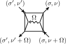
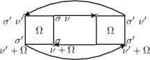
Figure 1: Left panel: Diagram notation for a dual fermion vertex. Two incoming lines with momenta/energies $\nu+\Omega$ and $\nu^{\prime}$ and spin $\sigma$ and $\sigma^{\prime}$ scatter into two outgoing lines with momenta $\nu^{\prime}+\Omega$ and $\nu$. A momentum $\Omega$ is transferred from right to left. Right panel: lowest order diagram. For clarity we omit the arrow inside the vertex.

III Stochastic Sampling of the Dual Fermion Series

In this work, we instead consider the full series of all dual diagrams with two-particle vertices using a stochastic diagrammatic Monte Carlo sampling procedure. We neglect three-particle and higher order impurity vertices. The diagram series is given by Eq. 10 and reads

$$\tilde{\Phi}=\sum_{n}\frac{1}{n!}\int_{C}\sum_{i^{(1)}=1}^{n}\sum_{i^{(2)}=1}^{n}\ldots\sum_{i^{(n)}=1}^{n}\prod_{k=1}^{n}\\ (-\frac{1}{4}\gamma_{i^{(k)}_{1234}}\xi_{i^{(k)}_{1}}\xi^{\dagger}_{i^{(k)}_{2}}\xi_{i^{(k)}_{3}}\xi^{\dagger}_{i^{(k)}_{4}})e^{-S^{d}_{0}\left[\xi^{\dagger},\xi\right]}D[\xi,\xi^{*}]\\ =\sum_{n}\sum_{i^{(1)}=1}^{n}\sum_{i^{(2)}=1}^{n}\ldots\sum_{i^{(n)}=1}^{n}\mathcal{W}_{n}(\mathcal{C}),$$ (11)

where the $i^{(m)}=(\nu_{m},\nu_{m}^{\prime},\sigma_{m},\sigma_{m}^{\prime})$ is a composite index for the $m$-th vertex, $\nu=(\omega,k)$, and $\mathcal{W}_{n}(\mathcal{C})$ is the contribution of the each term to the dual Luttinger-Ward functional: a Feynman diagram. These diagrams build the Monte Carlo configurations for our stochastic sampling. Each diagram evaluates to a (complex) number

$$\mathcal{W}_{n}(\mathcal{C})=\frac{(-1)^{n}}{n!}\left(\frac{1}{4}\right)^{n}\prod_{m=1}^{n}\gamma^{\sigma_{m}\sigma^{\prime}_{m}}_{\nu_{m}\nu^{\prime}_{m}\Omega_{m}}\tilde{G}_{\sigma_{m}}(\nu_{m})\times\\ \tilde{G}_{\sigma^{\prime}_{m}}(\nu^{\prime}_{m}+\Omega_{m})$$ (12)

and is uniquely defined by a graph: a set of interaction vertices connected by propagators, defined as $\langle\xi_{i_{m}}\xi^{\dagger}_{j_{m}}\rangle_{S_{0}}=-\tilde{G}_{\sigma_{m}}(\nu_{m})$ and appropriately anti-symmetrized vertex functions $\gamma^{\sigma_{m}\sigma^{\prime}_{m}}_{\nu_{m}\nu^{\prime}_{m}\Omega_{m}}=\gamma_{i^{m}}$. Momentum and energy are conserved at each vertex, and each vertex consists of a scattering process of two dual fermions with momentum transfer $\Omega$. The vertices are graphically illustrated in the left panel of Fig. 1: A dual particle with momentum end energy $\nu+\Omega$ and spin $\sigma$ scatters with a particle with momentum and energy $\nu^{\prime}$ and spin $\sigma^{\prime}$ and imparts on it a momentum/energy of $\Omega$. Vertices carry a weight $\frac{1}{4}\gamma_{\nu\nu^{\prime}\Omega}^{\sigma\sigma^{\prime}}$, each line carries spin and momentum/energy and evaluates to $\tilde{G}_{\sigma_{m}}(\nu_{m})$. A typical second order diagram is illustrated in the right panel of Fig. 1, where two vertices with identical momentum transfer and two fermion loops are present.

III.0.1 Monte Carlo sampling procedure

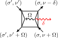
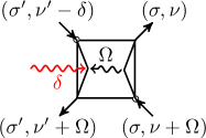
Figure 2: Auxiliary ‘worm’ diagrams. Left panel: a worm tail is attached to the spin-$\sigma$ line and carries away momentum $\delta$. Right panel: a worm head, attached to the spin $\sigma^{\prime}$ line, carries in momentum $\delta$ (right). Note that momentum is conserved at each vertex and head or tails can be attached to either line.

To stochastically sample all diagrams, we define a set of updates to change diagram order, diagram topology, the energy and momentum of propagators and vertices, as well as the spin of propagator lines, and perform a Markov chain Monte Carlo random walk in diagram space. Our method is an adaptation of the established diagrammatic Monte Carlo algorithmsProkof’ev and Svistunov (1998); Kozik et al. (2010); Houcke et al. (2010) but is formulated in Matsubara frequency rather than imaginary time space. To ensure that all possible diagrams are generated (ergodicity), while respecting spin, energy, and momentum conservation, we found it necessary to enlarge our space of diagrams and introduce “worms”:Prokof’ev and Svistunov (1998) auxiliary bosonic lines (of which we have at most one at any time) that carry momentum and frequency from one part of the diagram to another. These ‘worms’ are attached to two possible positions of our vertices, see Fig. 2 for an illustration. As the weight of a diagram in worm space we choose the product of propagator and vertex factors that we have in Luttinger-Ward diagram space, multiplied by a parameter $\eta$ which is chosen such that about equal time is spent in worm and Luttinger-Ward diagram space. A sequence of updates typically proceeds from a diagram, inserting a worm line with a random momentum and energy, using it to change topology or diagram order, and finally removing it. Unlike in other algorithms where worms represent Green’s function configurations, worm configurations have no physical meaning and are purely used as an auxiliary formulation to update diagrams. We found the following set of updates necessary to correctly generate all topologies: worm insertion and removal, worm move, change of topology, change of order, and spin-flip updates.

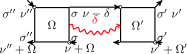
Figure 3: Two complementary ways of inserting an auxiliary ‘worm’ diagram line carrying momentum $\delta$ into a second order Luttinger-Ward diagram.

III.0.2 Insertion and Removal of a Worm

We start the discussion of the Monte Carlo updates with the insertion and removal of an auxiliary boson ‘worm’ line. This update transitions between Luttinger-Ward and worm space. For inserting a worm, we choose a random propagator and a random worm energy $\delta$, modify the propagator energy $\nu$ to $\nu-\delta$, attach the worm tail to the source of the propagator and the worm head to the target of the propagator. The resulting diagram conserves momentum and is illustrated in the left panel of Fig. 3. The reverse move takes an existing worm and proposes to remove it if it goes along a propagator, while changing the propagator energy from $\nu-\delta$ to $\nu$.

A second, complementary update inserts a worm with energy $\delta$ on a vertex or removes it from a vertex. In this case, the vertex frequency is modified from $\Omega$ to $\Omega-\delta$ (insertion) or $\Omega-\delta$ to $\Omega$ (removal). These updates are illustrated in the right panel of Fig. 3. Satisfying detailed balance requires taking into account the proper update proposal probabilities. We use Metropolis updates, for both updates the acceptance criteria are the same and given by

$$p^{\text{worm insert}}(\delta)=\min\left(1,\frac{p_{new}}{p_{old}}\frac{k}{p(\delta)}\eta\right)$$ (13)

$$p^{\text{worm remove}}(\delta)=\min\left(1,\frac{p_{new}}{p_{old}}\frac{p(\delta)}{k}\frac{1}{\eta}\right),$$ (14)

where $k$ denotes the expansion order and $p(\delta)$ the probability for proposing a random bosonic frequency $\delta$.

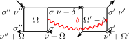
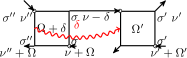
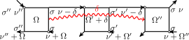
Figure 4: ‘worm move’ updates: starting from a worm configuration as in the left panel of Fig. 3, the worm head is (top left) moved across a vertex, changing its momentum transfer from $\Omega$ to $\Omega-\delta$, or (top right) its tail is moved across a vertex, changing its momentum from $\Omega$ to $\Omega+\delta$. Bottom panel: a worm head is moved along a propagator line, changing its momentum from $\nu^{\prime}$ to $\nu^{\prime}-\delta$.

III.0.3 Move of a worm

The worm ‘move’ update moves a worm head or tail along parts of the diagram. Several distinct possibilities exist: First, a worm ‘head’ is moved forward along an outgoing propagator line, in which case the value of the propagator is changed from $\nu$ to $\nu+\delta$. Second, a worm head is moved backward along an outgoing vertex line, in this case the value of the propagator is changed from $\nu$ to $\nu-\delta$. These two updates balance each other. Third, a worm tail is moved along an outgoing propagator line. In this case, the propagator’s energy is changed from $\nu$ to $\nu-\delta$. Fourth, a worm tail is moved backward along an incoming propagator line. In this case, the propagator’s energy is changed from $\nu$ to $\nu+\delta$. These updates, too, balance each other. Fifth, a worm head is moved from the right side of a vertex to the left side of a vertex, in which case the momentum transfer of that vertex is changed from $\Omega$ to $\Omega-\delta$. Sixth, a worm head is moved from the left side of a vertex to the right side of a vertex, in which case the momentum transfer of the vertex is changed from $\Omega$ to $\Omega+\delta$. Similar relations for the move of a worm tail across a vertex and for the move of a worm head or tail forward or backward along an incoming propagator line are easily derived. Fig. 4 illustrates some of these updates. As the proposal probability of a move and its inverse move are identical, no factors appear in the Metropolis criterion.

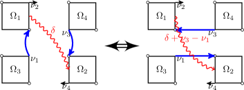
Figure 5: Updates changing diagram topology: A worm connecting two diagrams reconnects their outgoing vertex lines.

III.0.4 Change of topology

Changes of diagram topology are best done in worm space. To set the stage we assume an initial configuration in which a worm connects vertex $1$ to vertex $2$, with the incoming propagator (energy $\nu_{1}$) of vertex $1$ on the side of the worm pointing from vertex $3$ and the incoming propagator on vertex $2$ (energy $\nu_{3}$) pointing from vertex $4$. This configuration is shown in the left panel of Fig. 5. It is then possible to design an update that reconnects the propagator of vertex $4$ to vertex $1$ and of vertex $3$ to vertex $2$, as illustrated in the right panel of Fig. 5. Without the presence of a worm, such an update would most likely violate momentum conservation. Here, momentum conservation can be restored by changing the worm momentum from $\delta$ to $\delta+\nu_{3}-\nu_{1}$. This update is its own reverse update.

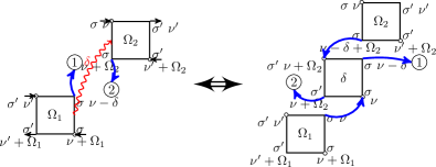
Figure 6: Updates changing diagram expansion order: As read from left to right: update changing a worm space configuration with $n$ vertices into a Luttinger-Ward diagram configuration with $n+1$ vertices, by inserting a new vertex with momentum transfer $\delta$. As read from right to left: update changing a Luttinger-Ward diagram configuration with $n+1$ vertices into a worm configuration with $n$ vertices by removing a vertex.

III.0.5 Change of diagram order

In order to change the diagram order of the expansion, we employ an update that takes a ‘worm’ diagram and inserts in its place a new vertex or, conversely, takes a Luttinger-Ward diagram configuration and replaces one of its vertices by a worm line. In this update, illustrated in Fig. 6, the worm momentum $\delta$ is converted into the vertex transfer momentum. Starting from a worm configuration connecting two vertices $1$ and $2$, the update consists of three steps. First, a new vertex with momentum transfer $\delta$ is created and its outgoing legs are connected to the targets of the outgoing legs of vertices $1$ and $2$. Second, the incoming legs of the new vertex are connected to the sources of the outgoing legs of vertices $1$ and $2$. Third, the momenta of the newly created legs are adjusted such that momentum conservation at each vertex is satisfied. The reverse update consists of selecting a vertex, replacing it by a worm line, and adjusting momenta such that momentum conservation is respected, as illustrated in the right panel of Fig. 6.

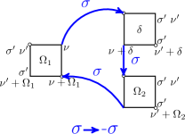
Figure 7: Example of a fermion loop identified by randomly selecting a propagator and following one of its fermion lines until it reaches the original vertex. The ‘spin flip’ update then proceeds by flipping the spin of all propagators and vertices along this loop.

III.0.6 Spin-flip update

Since new vertices always inherit the spins of the propagators from which they have been created, an additional update is necessary: the change of a fermion loop from spin $\sigma$ to spin $-\sigma$. For this purpose we identify a fermion loop by following the diagram along a propagator, without traversing a vertex, until the loop closes. Such a loop is non-local as it covers at least two vertices (Hartree and Fock diagrams are zero) but may cover a large fraction of the diagram vertices. We then propose to flip the spin of that propagator from $\sigma$ to $-\sigma$ and accept or reject according to the Metropolis criterion. Fig. 7 illustrates such a loop. This update is self-balanced.

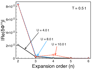
Figure 8: Contribution to the real part of the Luttinger-Ward functional of the dual fermion expansion as a function of diagram expansion order. Hubbard model, half filling, $T/t=0.5$ and $U/t=4.0,8.0,10.0$.

IV Results

In this section we present results obtained by the diagrammatic Monte Carlo dual fermion algorithm. We first illustrate the most important technical aspects of the diagrammatic sampling, then introduce results for the main quantity obtained in the algorithm: the dual self-energy, and finally present results for the physical self-energy and a comparison to results from another method. We defer a detailed analysis of the physics of the half-filled and doped two-dimensional Hubbard model to a later publication.

We start our discussion of the results with a plot for the contribution of diagrams at each order to the dual Luttinger-Ward functional for different interaction strength, Fig. 8, at a relatively high temperature $T/t=0.5$. At intermediate to weak coupling ($U/t=4$, black circles), second order corrections capture almost the entire difference to the DMFT result. Contributions of terms with more than three vertices are negligibly small. At an interaction strength of the bandwidth ($U/t=8$, blue squares), we find that second order contributions are still dominant, and the magnitude of their contribution has increased substantially. Fourth and higher order contributions are essentially zero. At an interaction strength larger than the bandwidth, $U/t=10$, deviations from diagrams containing more than three interaction vertices are visible, but the series is still convergent at an expansion order of five. Varying doping, temperature, and other parameters can push the series to regions where much higher order diagrams are important or where it eventually diverges.

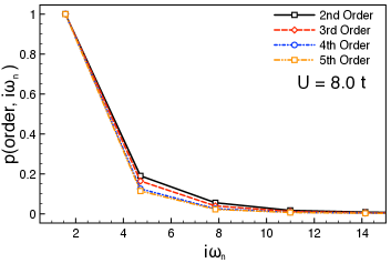
Figure 9: Probability that a dual diagram at order $2$, $3$, $4$, or $5$ contains propagators with frequency $i\omega_{n}$, normalized to the probability of a diagram at the same order containing a propagator at the lowest Matsubara frequency. Data for $T/t=0.5$ and $U/t=8.0$.

The Monte Carlo random walk automatically generates diagrams of the dual Luttinger Ward functional with the weight that they contribute to $\tilde{\Phi}$. Fig. 9 shows the distribution of propagator lines contained in the diagrams generated by the Monte Carlo random walk as a function of frequency, resolved by expansion order. As contributions from higher expansion orders are strongly suppressed (see Fig. 8), we normalize data for each order to the contribution of the lowest Matsubara frequency at that order.

It is apparent that only contributions from the lowest few Matsubara frequencies are generated, implying that contributions containing high frequency diagrams are strongly suppressed.

This strong suppression of higher Matsubara frequencies is a direct consequence of the fast decay of propagators $\sim\frac{1}{i\omega_{n}^{2}}$ (rather than $\sim\frac{1}{i\omega_{n}}$, as e.g. in a bare series) and presents a major difference to diagrammatic algorithms for bare fermionic series formulated in frequency space. At any order at temperature $T/t=0.5$, less than $\sim 4$ frequencies contribute significantly.

Decreasing temperature leads to an increase of the number of contributing Matsubara frequencies. This is shown in Fig. 10, where the frequency distribution in the weak and strong coupling regimes at two temperatures $T/t=0.5$ (left column) and $T/t=0.26$ and $T/t=0.2$ (right column) is plotted. Even at relatively small temperature there is no significant contribution from frequencies higher than $\omega_{n}\sim 12$ and the number of required frequencies depends on temperature as $\frac{1}{T}$, implying that the frequency scale of the non-local corrections stays small, so that dual fermion corrections only contribute at low frequencies.

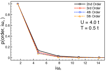
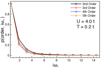
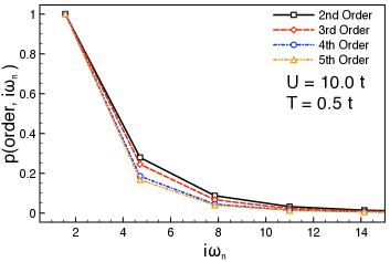
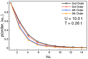
Figure 10: Probability that a dual diagram at order $2$, $3$, $4$, or $5$ contains propagators with frequency $i\omega_{n}$, normalized to the probability of a diagram at the same order containing a propagator at the lowest Matsubara frequency. Data for $U/t=4.0$ (upper row) and $U/t=10.0$ (lower row), for $T/t=0.5$ (left panel) and $T/t=0.2$ and $T/t=0.26$ (right panel).

This confinement of the series to low frequencies has practical consequences: it implies that the space needed to be sampled is small, so that the method converges quickly. It also shows the advantage of sampling diagrams directly in frequency, rather than in imaginary time space. Finally, because higher order impurity vertices are coupled to more propagator lines, one may expect that their contribution similarly is restricted to low frequencies, making their computation (and integration into our Monte Carlo method) feasible.

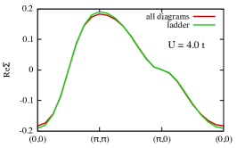
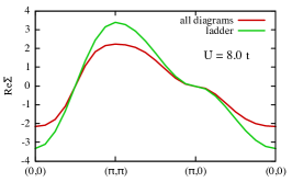
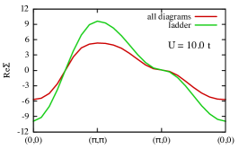
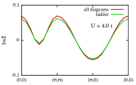
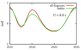
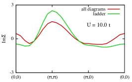
Figure 11: Real (upper row) and imaginary (lower row) part of the ladder dual self-energy (green lines) and real part of the self-energy from all diagrams sampled up to fifth order (red lines) plotted along the main axes of the Brillouin zone at the lowest Matsubara frequency, discretized on a $16\times 16$ grid of momenta and obtained at the coupling strengths $U/t=4$ (left column), $U/t=8$ (middle column) and $U/t=10$ (right column) and at $T/t=0.5$.

The main output of our simulation are the dual self-energies of Eq. 9, which are continuous functions of momentum and Matsubara frequency. These quantities are the input from which lattice Green’s functions, energies, and (lattice) self-energies are computed. We plot three examples of this quantity sampled up to the fifth order in Fig. 11 in comparison to the RPA-like ladder summation of the series obtained with the open source opendf code.Antipov et al. (2015) The resulting difference illustrates that in the very weak coupling regime (left panel, $U/t=4,T/t=0.5$), the series is dominated by a ladder contribution and non-ladder contributions are very small. As the interaction is changed to the intermediate (middle panel, $U/t=8$) and strong coupling (right panel, $U/t=10$) regime, the non-ladder contributions become substantial, illustrating the importance of our diagrammatic procedure that samples all possible contributions of two-particle vertex diagrams.

The lattice self-energy extracted from the dual self-energy for weak coupling shown in Fig. 11 is shown in Fig. 12. We show results for the real part of the self-energy and results from 2nd, 3rd, and 4th order of diagrammatic dual Fermions. Our results are compared to 64-site dynamical cluster approximation (DCA) data of Ref. LeBlanc et al., 2015; LeBlanc and Gull, 2013 which yield a step-wise constant self-energy. For these parameters, the system is above any antiferromagnetic ordering temperature (in DMFT or DCA or dual Fermions). The particle hole symmetry is visible as a symmetry between $(0,0)$ and $(\pi,\pi)$, but antiferromagnetic fluctuations are large and long ranged. Convergence to the DCA solution for these parameters is clearly visible, and the dual Fermion results provide valuable additional momentum resolution of the self-energy that may in the future allow the resolution of subtle k-space features.

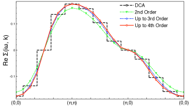
Figure 12: Real part of the lattice self-energy plotted along the main axes of the Brillouin zone at the lowest Matsubara frequency, discretized on a $16\times 16$ grid of momenta and obtained for the weak coupling strength $U/t=4$ at $T/t=0.5$, and evaluated up to second order (triangles, green lines), third order (diamonds, blue lines), and 4th order (circles, red lines). Black squares: Comparison to the piecewise constant real self-energy obtained from a dynamical cluster approximation calculation of the same system obtained on a $64$-site cluster.

The computational cost of diagrammatic Monte Carlo dual fermion calculations is low compared to other methods for correlated systems. The numerical effort for evaluating the series for parameters examined in this paper ranges from a few minutes for cases where DMFT is accurate to a few hours for cases where the expansion order is high. The computational effort of computing the DMFT vertex functions is strongly dependent on the number of frequencies kept and increases rapidly as $T$ is lowered.

V Conclusions

In conclusion, we have applied a Diagrammatic Monte Carlo method to sample the dual fermion corrections to the dynamical mean field theory and shown results for the two-dimensional Hubbard model at half filling at small, intermediate and large values of interaction strength. While the method includes all diagram topologies with two-particle vertices, higher order vertices are neglected. As $T$ is lowered or $U$ changed towards the intermediate interaction regime, non-local contributions beyond second order become relevant. All corrections are limited to a comparatively narrow frequency range. These contributions contain a substantial part of non-ladder diagrams, illustrating that all diagram topologies contribute substantially away from weak coupling and critical regimes. The low frequency scale of these diagrams offers the possibility that three-particle and higher order vertices may be included in future work.