Electrical conductivity of hadronic matter from different possible mesonic and baryonic thermal fluctuations

Abstract

Electromagnetic current-current correlators in pionic and nucleonic medium have been evaluated in the static limit to obtain electrical conductivities for pion and nucleon components respectively, where former decreases and latter one increases with the variation of temperature $T$ and baryon chemical potential $\mu_{N}$. Therefore, total electrical conductivity of pion and nucleon system exhibits a valley structure in the $T$-$\mu_{N}$ plane. To get non-divergent and finite values of correlators, finite thermal widths of medium constituents, pion and nucleon have been considered, where these thermal widths have been determined from the in-medium scattering probabilities of pion and nucleon with other mesonic and baryonic resonances, based on effective hadronic model. At $\mu_{N}=0$, the results of present work are more or less agrees with the results of earlier works and its finite $\mu_{N}$ extension show a decreasing nature of electrical conductivity for hadronic medium during spanning from freeze out line to quark-hadron transition line in $T$-$\mu_{N}$ plane.

I Introduction

The electromagnetic current-current correlator at finite temperature is one of the very important quantity to characterize the medium, produced in high energy heavy ion collisions. The explicit dynamical structure of this quantity for hadronic matter (HM) is directly linked with the in-medium spectral function of neutral vector mesons and also with the thermal dilepton and photon yields from HM sources, whereas its static limit provide the estimation of an important transport coefficients like electrical conductivity ($\sigma$) of the HM. According to recent reviews Rapp_rev ; G_rev , the effective field theoretical calculations of hadrons at finite temperature are very successful to describe the low mass dimuon enhancement measured by the NA60 collaboration SPS . This low mass enhancement also get boost from the quark matter (QM) sources, which has been calculated by using Hard Thermal Loop (HTL) technique in Ref. HTL (see also Ref. Sarbani for effective QCD model calculation). Therefore, it will be very interesting and phenomenologically important to know the static limit estimation of the dynamical structure of current-current correlator by calculating $\sigma$ of hadronic medium in the frame work of effective hadronic model, which is basically attempted by this present work.

The event by event analysis Sokov in relativistic heavy ion collisions indicates about the possibility of generation of a high strength electric ($E$) and magnetic ($B$) fields in the medium. For example, in the relativistic heavy ion collider (RHIC) experiment, their approximate values are $eB\approx m_{\pi}^{2}\approx 10^{18}G$ and $eE\approx m_{\pi}^{2}\approx 10^{21}V/cm$ Tuchin . Although a particular magnetic field component becomes only non-zero in the average scenario Sokov ; Tuchin . The time evolution of this average magnetic field Tuchin depends on the $\sigma$ of the expanding medium, produced in heavy ion collisions, which demands that we should have some good idea on numerical values of this $\sigma$.

In Ref. Akamatsu , the electrical conductivity or electric charge diffusion coefficient of evolving medium is used as input to explain the low mass dilepton enhancement, observed experimentally by PHENIX collaboration at RHIC. Whereas, Yin Yin have shown that the electrical conductivity of quark-gluon-plasma (QGP) plays important role to regulate the soft photon production via realistic hydrodynamics simulation. Besides these indirect estimation of electrical conductivity of QGP, it can directly be extracted from charge dependent direct flow parameters in asymmetric heavy-ion (Au+Cu) collisions Hirano . Along with these phenomenological searching, different microscopic calculations for $\sigma$ of quark  Cassing ; Marty ; Puglisi ; Greif ; PKS ; Finazzo and hadronic phase Lee ; Nicola_PRD ; Nicola ; Greif2 have been done, although the results of Cassing et al Cassing in the model of PHSD (parton hadron string dynamics) and the NJL (Nambu-Jona-Lasino) model results of Marty et al. Marty have covered $\sigma$ estimation for the temperature domain of both quark and hadronic matter. On this problems, a large number of Lattice QCD calculations have been done LQCD_Ding ; LQCD_Arts_2007 ; LQCD_Buividovich ; LQCD_Burnier ; LQCD_Gupta ; LQCD_Barndt ; LQCD_Amato , where their estimations cover a large numerical band (see table 1, addressed in result section). Now, from the calculations Lee ; Nicola_PRD ; Nicola ; Greif2 in the hadronic temperature domain, we see that the results of Ref. Lee and Refs. Nicola_PRD ; Nicola ; Greif2 show completely opposite nature of temperature ($T$) dependence of $\sigma$. If we considered the results of Lee et al. Lee as an exceptional, almost all of the earlier works Cassing ; Marty ; Puglisi ; Greif ; PKS ; Finazzo ; Nicola_PRD ; Nicola ; Greif2 ; LQCD_Amato indicates that $\sigma/T$ decreases in hadronic temperature domain Cassing ; Marty ; Nicola_PRD ; Nicola ; Greif2 and increases in the temperature domain of quark phase Cassing ; Marty ; Puglisi ; Greif ; PKS ; Finazzo ; LQCD_Amato . Their numerical values are located within the order - $\sigma/T\approx 10^{-3}$ to $10^{-2}$ for hadronic phase and $\sigma/T\approx 10^{-3}$ to $10^{-1}$ for quark phase. These information from earlier studies indicate that the numerical strength as well as the nature of $\sigma(T)$ both are not very settle issue till now.

In this context, the present investigation is similar kind of microscopic calculations for $\sigma$, which is expected to converge and update our understanding of $\sigma(T)$. Considering pion and nucleon as abundant constituents of hadronic matter, we have calculated their electromagnetic current-current correlators at finite temperature, whose static limit give the estimation of $\sigma$ for the respective components. As an interaction part, the effective hadronic Lagrangian densities have been used to calculate the in-medium scattering probabilities of pion and nucleon with other mesonic and baryonic resonances, present in the hadronic medium. Extending our investigations for finite nucleon or baryon chemical potential $\mu_{N}$, the present results provide the estimation of $\sigma$ in $T$-$\mu_{N}$ domain of hadronic matter.

The basic formalism of $\sigma$ is addressed in the Sec. II, where we will see that the non-divergent values of current-current correlator are mainly regulated by the thermal widths of medium components, which are calculated and briefly described in Sec. III. Calculations of different loop diagrams are classified in three subsections. After it, the numerical discussions have been addressed in the result section (Sec. IV), which is followed by a summary in Sec. V.

II Formalism of electrical conductivity

Owing to the famous Kubo formula Zubarev ; Kubo , the electrical conductivity in momentum space can be expressed in terms of spectral density of current current correlator as Nicola

$$\sigma=\frac{1}{6}\lim_{q_{0},\vec{q}\rightarrow 0}\frac{A_{\sigma}(q_{0},\vec{q})}{q_{0}}$$ (1)

where $A_{\sigma}(q_{0},\vec{q})=\int d^{4}xe^{iq\cdot x}\langle[J^{\rm EM}_{i}(x),J^{i}_{EM}(0)]\rangle_{\beta}$ with $\langle..\rangle_{\beta}$ denotes the thermodynamical ensemble average.

In real-time thermal field-theory (RTF), any two point function at finite temperature always gives a $2\times 2$ matrix structure. Hence, the thermal correlator of electromagnetic current ($J^{\rm EM}_{\mu}(x)$) will be

$$\Pi^{ab}(q)=i\int d^{4}xe^{iqx}\langle T_{c}J^{\rm EM}_{\mu}(x)J_{\rm EM}^{\mu}(0)\rangle^{ab}_{\beta}~{},$$ (2)

where $T_{c}$ denotes the time ordering with respect to a symmetric contour in the complex time plane. Because of the contour, we get four possible set of two points and Therefore we get $2\times 2$ matrix structure of two point function. The superscripts $a,b(=1,2)$ in Eq. (2) represent the (thermal) indices of the matrix. Retarded part of correlator $\Pi^{R}(q)$ and its corresponding spectral density $A_{\sigma}(q)$ can be extracted from 11-component $\Pi^{11}(q)$ by using the relation

$$A_{\sigma}(q)=2{\rm Im}\Pi^{R}(q)=2{\rm tanh}(\frac{\beta q_{0}}{2}){\rm Im}\Pi_{11}(q)~{}.$$ (3)

Using this relation (3), the Eq. (1) can alternatively be expressed as

$$\sigma = \frac{1}{3}\lim_{q_{0},\vec{q}\rightarrow 0}\frac{{\rm Im}\Pi^{R}(q_{0},\vec{q})}{q_{0}}$$ (4)

$$= \frac{1}{3}\lim_{q_{0},\vec{q}\rightarrow 0}\frac{{\rm tanh}(\frac{\beta q_{0}}{2}){\rm Im}\Pi^{11}(q_{0},\vec{q})}{q_{0}}~{}.$$

Since pion and nucleon constituents are our matter of interest, so we should focus on their electromagnetic currents:

$$J^{\mu}_{\pi} = e\phi_{\pi}(\partial^{\mu}\phi_{\pi})$$

$${\rm and}~{}J^{\mu}_{N} = e{\overline{\psi}}_{N}\gamma^{\mu}\psi_{N}~{},$$ (5)

which are electromagnetically coupled with photon via interaction (QED) Lagrangian density

$${\cal L}=-(J^{\mu}_{\pi}+J^{\mu}_{N})A_{\mu}~{}.$$ (6)

Since ($\phi_{\pi^{+}}$, $\phi_{\pi^{-}}$) from pion triplet ($\phi_{\pi^{+}}$, $\phi_{\pi^{-}}$, $\phi_{\pi^{0}}$) and proton ($\psi_{p}$) from nucleon doublet ($\psi_{p}$, $\psi_{n}$) have non-zero electric charges, so we have to keep in mind about relevant isospin factors $I^{e}_{\pi}=2$ and $I^{e}_{N}=1$, which should be multiplied during our calculations.

To calculate electrical conductivity of pionic ($\sigma_{\pi}$) and nucleonic ($\sigma_{N}$) medium from their corresponding spectral density or retarded part of correlator via Eq. (4), let us start from 11-component of the $\Pi_{ab}$ matrix. The Wick contraction (see Appendix VI.1 ) of the pion ($\phi_{\pi}$) and nucleon ($\psi_{N}$) fields give one-loop diagrams of photon self-energy, which are shown in Fig. 1(a) and  2(a) respectively. A general mathematical expression of these diagrams is

$$\Pi^{11}(q)=ie^{2}\int\frac{d^{4}k}{(2\pi)^{4}}N~{}D^{11}(k)D^{11}(p)~{},$$ (7)

where $D^{11}(k)$ and $D^{11}(p)$ are the scalar parts of propagators, appeared in RTF for 11-component; $p=q-k$ for $\pi\pi$ loop in Fig. 1(a), $p=q+k$ for $NN$ loop in Fig. 2(a). Multiplication of vertex part and numerator part of two propagators build the term $N$.

In RTF, a general form of $D^{11}(k)$ for boson or fermion is

$$D^{11}(k) = \frac{-1}{k_{0}^{2}-\omega_{k}^{2}+i\epsilon}+2\pi i\epsilon_{k}F_{k}(k_{0})\delta(k_{0}^{2}-\omega_{k}^{2})~{},$$ (8)

$$~{}{\rm with}~{}F_{k}(k_{0})=n^{+}_{k}\theta(k_{0})+n^{-}_{k}\theta(-k_{0})~{},$$

where $n^{\pm}_{k}(\omega_{k})=\frac{1}{e^{\beta(\omega_{k}\mp\mu)}-\epsilon_{k}}$ are the thermal distribution functions and $\pm$ sign in the superscript of $n_{k}$ stand for particle and anti-particle respectively. Now when we proceed for special cases - pion (boson) or nucleon (fermion) field, we have to put

$$\epsilon_{k}=+1,~{}\mu=\mu_{\pi}=0~{}{\rm i.e.}~{}n^{+}_{k}=n^{-}_{k}~{},$$

$$\omega_{k}=\omega^{\pi}_{k}=(\vec{k}^{2}+m_{\pi}^{2})^{1/2}~{}{\rm for~{}pion}~{},$$ (9)

$$\epsilon_{k}=-1,~{}\mu=\mu_{N}~{}({\rm nucleon~{}chemical~{}potential})~{},$$

$$\omega_{k}=\omega^{N}_{k}=(\vec{k}^{2}+m_{N}^{2})^{1/2}~{}{\rm for~{}nucleon}~{}.$$ (10)

However, for time being we will will continue our calculation with the general form of $D^{11}$ from Eq. (8) and at latter stage, we will put these conditions (9) and (10) in the general expression.

Figure 1: The diagram (a) is a schematic one-loop representation of electromagnetic current-current correlator for the medium with pionic constituents. The external photon lines are coupled with double dashed internal lines of pions, which have some finite thermal width. Thermal width of pion can be derived from its self-energy diagrams (b), (c) and (d), where (b) represents pion self-energy for mesonic ($\pi M$) loops, whereas diagrams (c) and (d) are direct and cross diagrams of pion self-energy for $NB$ loops.

Figure 2: The diagram (a) is a schematic one-loop representation of electromagnetic current-current correlator for the medium with nucleonic constituents. Similar to double dashed lines of pions in Fig. (1), here double solid lines of nucleon indicates that they have finite thermal width, which can be obtained from the nucleon self-energy diagram (b) for $\pi B$ loops.

After using (8) in Eq. (7), if we do its $k_{0}$ integration and put it in Eq. (4), then we will get spectral density of electromagnetic current-current correlator G_IJMPA :

$$A_{\sigma}(q) = e^{2}\int\frac{d^{3}k}{(2\pi)^{3}}\frac{(-\pi)N}{4\omega_{k}\omega_{p}}[C_{1}\delta(q_{0}-\omega_{k}-\omega_{p})$$ (11)

$$+C_{2}\delta(q_{0}-\omega_{k}+\omega_{p})+C_{3}\delta(q_{0}+\omega_{k}-\omega_{p})$$

$$+C_{4}\delta(q_{0}+\omega_{k}+\omega_{p})]~{},$$

where $\omega_{p}=\omega_{p}^{\pi}=\{(\vec{q}-\vec{k})^{2}+m^{2}_{\pi}\}^{1/2}$ for pion field, $\omega_{p}=\omega_{p}^{N}=\{(\vec{q}+\vec{k})^{2}+m^{2}_{N}\}^{1/2}$ for nucleon field. Here $N$ are space component of $N(q,k_{0}=\pm\omega_{k},\vec{k})$ (see Appendix  VI.1):

$$N=(-4)\{-\vec{k}\cdot\vec{q}+\vec{k}^{2}\}~{}{\rm for}~{}\pi\pi~{}{\rm loop}~{},$$ (12)

and

$$N = (-8)\{\vec{k}\cdot\vec{q}+\vec{k}^{2}\}+4\vec{k}\cdot\vec{q}~{}{\rm for}~{}NN~{}{\rm loop}~{}.$$ (13)

The statistical probabilities, attached with four different delta functions, are

$$C_{1} = 1+n^{+}_{k}(\omega_{k})+n^{+}_{p}(q_{0}-\omega_{k})~{},$$

$$C_{2} = -n^{+}_{k}(\omega_{k})+n^{-}_{p}(-q_{0}+\omega_{k})~{},$$

$$C_{3} = n^{-}_{k}(\omega_{k})-n^{+}_{p}(q_{0}+\omega_{k})~{},$$

$$C_{4} = -1-n^{-}_{k}(\omega_{k})-n^{-}_{p}(-q_{0}-\omega_{k})~{},~{}{\rm for}~{}\pi\pi~{}{\rm loop}~{};$$

and

$$C_{1} = -1+n^{-}_{k}(\omega_{k})+n^{+}_{p}(q_{0}+\omega_{k})~{},$$

$$C_{2} = -n^{-}_{k}(\omega_{k})+n^{-}_{p}(-q_{0}+\omega_{k})~{},$$

$$C_{3} = n^{+}_{k}(\omega_{k})-n^{+}_{p}(q_{0}+\omega_{k})~{},$$

$$C_{4} = 1-n^{+}_{k}(\omega_{k})-n^{-}_{p}(-q_{0}-\omega_{k})~{},~{}{\rm for}~{}NN~{}{\rm loop}~{}.$$

Four different delta functions are responsible for creating four different regions of branch cuts in $q_{0}$-axis, where $A_{\sigma}(q_{0},\vec{q})$ or Im$\Pi^{R}(q_{0},\vec{q})$ becomes non-zero. These regions are

$$q_{0} = -\infty~{}~{}~{}{\rm to}~{}~{}~{}-\{\vec{q}^{2}+4m_{\pi,N}^{2}\}^{1/2}~{}:~{}{\rm unitary~{}cut}~{},$$ (18)

$$= \left.\begin{array}[]{c}-|\vec{q}|~{}~{}~{}~{}~{}{\rm to}~{}~{}~{}~{}~{}0\\ ~{}~{}~{}0~{}~{}~{}~{}~{}{\rm to}~{}~{}~{}~{}~{}|\vec{q}|\end{array}\right\}~{}:~{}{\rm Landau~{}cut}~{},$$

$$= \{\vec{q}^{2}+4m_{\pi,N}^{2}\}^{1/2}~{}~{}~{}{\rm to}~{}~{}~{}\infty~{}:~{}{\rm unitary~{}cut}~{}.$$ (19)

Since electrical conductivity $\sigma$ is the limiting value of $A_{\sigma}(q_{0},\vec{q})$ or Im$\Pi^{R}(q_{0},\vec{q})$ at $q_{0},\vec{q}\rightarrow 0$, therefore we should focus on Landau cuts only. Hence, using the Landau part of Eq. (11) in Eq. (1), we have

$$\sigma = \frac{e^{2}}{3}\lim_{q_{0},\vec{q}\rightarrow 0}\frac{1}{q_{0}}\int\frac{d^{3}k}{(2\pi)^{3}}\frac{(-\pi)N}{4\omega_{k}\omega_{p}}\{C_{2}\delta(q_{0}-\omega_{k}+\omega_{p})$$

$$+C_{3}\delta(q_{0}+\omega_{k}-\omega_{p})\}$$

$$= \frac{e^{2}}{3}\lim_{q_{0},\vec{q}\rightarrow 0}{\rm Im}\left[\int\frac{d^{3}k}{(2\pi)^{3}}\frac{N}{4\omega_{k}\omega_{p}}\lim_{\Gamma\rightarrow 0}\right.$$

$$\left.\left\{\frac{C_{2}/q_{0}}{(q_{0}-\omega_{k}+\omega_{p})+i\Gamma}+\frac{C_{3}/q_{0}}{(q_{0}+\omega_{k}-\omega_{p})+i\Gamma}\right\}\right]~{}.$$

We will take finite value of $\Gamma$ in our further calculations to get a non-divergent values of $\sigma$. In Kubo approach, this traditional technique is widely used to calculate different transport coefficients like shear viscosity Nicola ; G_IJMPA , electrical conductivity Nicola_PRD . In this respect, this formalism is very much close to quasi particle approximation. The $\Gamma$ of medium constituents is basically their thermal width, which is physically related with the probabilities of different in-medium scattering. Inverse of $\Gamma$ measures the relaxation time $\tau$, which is the average time of medium constituents to reach their equilibrium conditions.

Next, applying the L’Hospital’s rule in the Eq. (LABEL:el_G) (see Appendix  VI.2), we get a generalized expression of electrical conductivity for bosonic ($\phi_{\pi}$) or fermionic ($\psi_{N}$) field:

$$\sigma=\frac{\beta e^{2}}{3}\int\frac{d^{3}k}{(2\pi)^{3}}\frac{(-N^{0})}{4\omega_{k}^{2}\Gamma}[n^{-}_{k}(1+\epsilon_{k}n^{-}_{k})+n^{+}_{k}(1+\epsilon_{k}n^{+}_{k})]~{},$$ (21)

where

$$N^{0}=\lim_{q_{0},\vec{q}\rightarrow 0}N(k_{0}=\pm\omega_{k},\vec{k},q)~{}.$$ (22)

Depending upon the sign of $\epsilon_{k}$, the statistical probability becomes Bose enhanced ($\epsilon_{k}=+1$ for bosonic field) or Pauli blocked ($\epsilon_{k}=-1$ for fermionic field) probability. Following the definition of $N^{0}$ in Eq. (22), Eqs. (12) and (13) can be simplified as

$$N^{0}=-I^{e}_{\pi}(4\vec{k}^{2})~{}~{}~{}{\rm for~{}}\pi\pi~{}{\rm loop}~{},$$ (23)

and

$$N^{0}=-I^{e}_{N}(8\vec{k}^{2})~{}~{}~{}{\rm for~{}}NN~{}{\rm loop}~{}.$$ (24)

Using the above Eqs. (23) and (24) in Eq. (21) as well as their relevant parameters from Eq. (9) and (10), we get the electrical conductivity of the pionic and nucleonic medium:

$$\sigma_{\pi}=\frac{\beta e^{2}}{3}\int^{\infty}_{0}\frac{d^{3}\vec{k}}{(2\pi)^{3}}\frac{\vec{k}^{2}}{{\omega^{\pi}_{k}}^{2}\Gamma_{\pi}}n_{k}(\omega^{\pi}_{k})\{1+n_{k}(\omega_{k}^{\pi})\}$$ (25)

and

$$\sigma_{N} = \frac{2\beta e^{2}}{3}\int^{\infty}_{0}\frac{d^{3}\vec{k}}{(2\pi)^{3}}\frac{\vec{k}^{2}}{{\omega^{N}_{k}}^{2}\Gamma_{N}}[n^{+}_{k}(\omega_{k}^{N})\{1-n^{+}_{k}(\omega^{N}_{k})\}$$ (26)

$$+n^{-}_{k}(\omega^{N}_{k})\{1-n^{-}_{k}(\omega^{N}_{k})\}]~{}.$$

Hence, adding the pionic and nucleonic components, we get the total electrical conductivity

$$\sigma_{\rm T}=\sigma_{\pi}+\sigma_{N}~{}.$$ (27)

III Thermal width

Let us come to the thermal widths of pion ($\Gamma_{\pi}$) and nucleon ($\Gamma_{N}$). Pion thermal width can be obtained from the imaginary part of pion self-energy for different mesonic and baryonic fluctuations. Fig. 1(b) represents pion self-energy diagram for $\pi M$ (mesonic) loops - ${\Pi}^{R}_{\pi(\pi M)}$, where $M=\sigma,~{}\rho$. Here subscript in ${\Pi}^{R}_{\pi(\pi M)}$ stands for the external (outside the bracket) and internal (inside the bracket) particles for the diagram 1(b). This notation will be followed by latter diagrams also. Now, pion self-energy for different baryonic loops (${\Pi}^{R}_{\pi(NB)}$) can have two possible diagrams as shown in Fig. 1(c) and (d). Here internal lines $NB$ stand for nucleon ($N$) and baryon ($B$) respectively, where different 4-star spin $1/2$ and $3/2$ baryons are taken in our calculations. Adding all those mesonic and baryonic loops, we get total thermal width of pion $\Gamma_{\pi}$, which can be expressed as

$$\Gamma_{\pi} = \sum_{M}\Gamma_{\pi(\pi M)}+\sum_{B}\Gamma_{\pi(NB)}$$ (28)

$$= -\sum_{M}{\rm Im}{\Pi}^{R}_{\pi(\pi M)}(k_{0}=\omega^{\pi}_{k},\vec{k})/m_{\pi}$$

$$~{}~{}~{}-\sum_{B}{\rm Im}{\Pi}^{R}_{\pi(NB)}(k_{0}=\omega^{\pi}_{k},\vec{k})/m_{\pi}~{}.$$

Similarly, nucleon self-energy is shown in Fig. 2(b) and it has been denoted as $\Sigma^{R}_{N(\pi B)}$, where in internal lines, we have taken all those spin $1/2$ and $3/2$ baryons ($B$) as taken in pion self-energy for baryonic loops. Hence, summing these all $\pi B$ loops, we can express our nucleon thermal width as

$$\Gamma_{N}=\sum_{B}\Gamma_{N(\pi B)}=-\sum_{B}{\rm Im}\Sigma^{R}_{N(\pi B)}(k_{0}=\omega^{N}_{k},\vec{k})~{}.$$ (29)

Next we discuss briefly the calculations of thermal widths from different one-loop self-energy graphs as shown in Fig. (1) and (2).

III.1 Pion thermal width for different mesonic loops

To calculate the mesonic loop contribution of pionic thermal width $\Gamma_{\pi(\pi M)}$, the pion self-energy for $\pi M$ loops, where $M$ stands for $\sigma$ and $\rho$ mesons, have been evaluated and it is expressed as GKS

$$\Gamma_{\pi(\pi M)} = {\rm Im}{\Pi}^{R}_{\pi(\pi M)}(k_{0}=\omega^{\pi}_{k},\vec{k})/m_{\pi}$$ (30)

$$= \frac{1}{m_{\pi}}\int\frac{d^{3}\vec{l}}{32\pi^{2}\omega_{l}^{\pi}\omega_{u}^{M}}$$

$$L(l_{0}=-\omega^{\pi}_{l},\vec{l},k_{0}=\omega^{\pi}_{k},\vec{k})\{n(\omega^{\pi}_{l})$$

$$-n(\omega^{M}_{u})\}\delta(\omega^{\pi}_{k}+\omega^{\pi}_{l}-\omega^{M}_{u})~{},$$

where $n(\omega^{\pi}_{l})$, $n(\omega^{M}_{u})$ are BE distribution functions of $\pi$, $M$ mesons with energies $\omega^{\pi}_{l}=(\vec{l}^{2}+m_{\pi}^{2})^{1/2}$ and $\omega^{M}_{u}=(|\vec{k}-\vec{l}|^{2}+m_{M}^{2})^{1/2}$ respectively. The vertex factors $L(k,l)$ GKS have been obtained from the effective Lagrangian density,

$${\cal L}=g_{\rho}\,{\vec{\rho}}_{\mu}\cdot{\vec{\pi}}\times\partial^{\mu}{\vec{\pi}}+\frac{g_{\sigma}}{2}m_{\sigma}{\vec{\pi}}\cdot{\vec{\pi}}\,\sigma~{}.$$ (31)

III.2 Pion thermal width for different baryonic loops

Along with the mesonic fluctuations, different baryon fluctuations may provide some contributions in pion thermal width. This component can be derived from pion self-energy for different $NB$ loops, where $B=N(940)$, $\Delta(1232)$, $N^{*}(1440)$, $N^{*}(1520)$, $N^{*}(1535)$, $\Delta^{*}(1600)$, $\Delta^{*}(1620)$, $N^{*}(1650)$, $\Delta^{*}(1700)$, $N^{*}(1700)$, $N^{*}(1710)$, $N^{*}(1720)$ are taken G_pi_JPG ; G_eta_BJP . The masses of all the 4-star baryon resonances (in MeV) are presented inside the brackets. The direct and cross diagrams of pion self-energy for $NB$ loops are shown in Fig. 1(c) and (d). Adding the relevant Landau cut contributions of both diagrams (c) and (d), the total thermal width of pion for any $NB$ loop is given by G_pi_JPG ; G_eta_BJP

$$\Gamma_{\pi(NB)} = {\rm Im}{\Pi}^{R}_{\pi(NB)}(k_{0}=\omega^{\pi}_{k},\vec{k})/m_{\pi}$$ (32)

$$= \frac{1}{m_{\pi}}\int\frac{d^{3}\vec{l}}{32\pi^{2}\omega_{l}^{N}\omega_{u}^{B}}$$

$$[L(l_{0}=\omega^{N}_{l},\vec{l},k_{0}=\omega_{k}^{\pi},\vec{k})\{n^{+}_{l}(\omega^{N}_{l})$$

$$-n^{+}_{u}(\omega^{B}_{u})\}\delta(\omega^{\pi}_{k}-\omega^{N}_{l}+\omega^{B}_{u})$$

$$+L(l_{0}=-\omega^{N}_{l},\vec{l},k_{0}=\omega_{k}^{\pi},\vec{k})\{-n^{-}_{l}(\omega^{N}_{l})$$

$$+n^{-}_{u}(\omega^{B}_{u})\}\delta(\omega^{\pi}_{k}+\omega^{N}_{l}-\omega^{B}_{u})]~{},$$

where $n^{\pm}(\omega^{N}_{l})$, $n^{\pm}(\omega^{B}_{u})$ are FD distribution functions of $N$, $B$ ($\pm$ for particle and anti-particle) with energies $\omega^{N}_{l}=(\vec{l}^{2}+m_{N}^{2})^{1/2}$ and $\omega^{B}_{u}=(|\pm\vec{k}+\vec{l}|^{2}+m_{B}^{2})^{1/2}$ ($\pm$ for two different diagrams) respectively.

With the help of the effective Lagrangian densities Leopold ,

$${\cal L} = \frac{f}{m_{\pi}}{\overline{\psi}}_{B}\gamma^{\mu}\left\{\begin{array}[]{c}i\gamma^{5}\\ 1\!\!1\end{array}\right\}\psi_{N}\partial_{\mu}\pi+{\rm h.c.}~{}{\rm for}~{}J_{B}^{P}=\frac{1}{2}^{\pm},$$ (35)

$${\cal L} = \frac{f}{m_{\pi}}{\overline{\psi}}^{\mu}_{B}\left\{\begin{array}[]{c}1\!\!1\\ i\gamma^{5}\end{array}\right\}\psi_{N}\partial_{\mu}\pi+{\rm h.c.}~{}{\rm for}~{}J_{B}^{P}=\frac{3}{2}^{\pm},$$ (38)

the vertex factors $L(k,l)$ G_pi_JPG ; G_eta_BJP can be found.

III.3 Nucleon thermal width

The nucleonic thermal width has been calculated from nucleon self-energy for different possible $\pi B$ loops, where $B$ stands for all the baryons as taken in pion self-energy for baryonic loops. Evaluating the loop diagram, shown in Fig. 2(b), we get G_NNst_BJP ; G_N

$$\Gamma_{N(\pi B)} = -\sum_{B}{\rm Im}\Sigma^{R}_{N(\pi B)}(k_{0}=\omega^{N}_{k},\vec{k})$$ (39)

$$= \int\frac{d^{3}\vec{l}}{32\pi^{2}\omega_{l}^{\pi}\omega_{u}^{B}}$$

$$L(l_{0}=-\omega^{\pi}_{l},\vec{l},k_{0}=\omega_{k}^{N},\vec{k})\{n(\omega^{\pi}_{l})$$

$$+n^{+}(\omega^{B}_{u})\}\delta(\omega^{N}_{k}+\omega^{\pi}_{l}-\omega^{B}_{u})$$

where $n(\omega^{\pi}_{l})$ and $n^{+}(\omega^{B}_{u})$ are BE and FD distribution functions for $\pi$ and $B$ with energies $\omega_{l}^{\pi}=(\vec{l}^{2}+m_{\pi}^{2})^{1/2}$ and $\omega^{B}_{u}=(|\vec{k}-\vec{l}|^{2}+m_{B}^{2})^{1/2}$ respectively.

The vertex factors $L(k,l)$ G_NNst_BJP ; G_N can be deduced by using the $\pi NB$ interaction Lagrangian densities from Eq. (38).

IV Results and Discussion

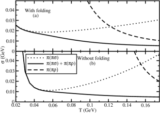
Figure 3: Temperature dependence of electrical conductivity pionic medium due to its different mesonic fluctuations - $\pi\sigma$ (dotted line), $\pi\rho$ (dashed line) loops and their total (solid line). With and without folding effect of resonances $M=\sigma,\rho$ are taken in upper and lower panels respectively.

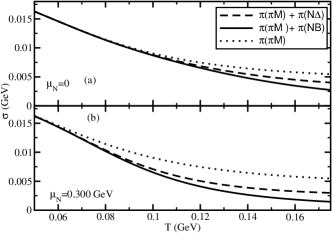
Figure 4: Effect of baryonic fluctuations ($N\Delta$ loop : dashed line, $NB$ loops : solid line) after adding with mesonic fluctuations ($\pi M$ loops : dotted line) of pion on $\sigma_{\pi}(T)$ at $\mu_{N}=0$ (a) and $\mu_{N}=0.300$ GeV (b).

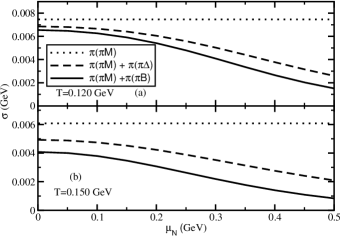
Figure 5: Same as Fig. (4) for $\sigma_{\pi}(\mu_{N})$ at $T=0.120$ GeV (a) and $T=0.150$ GeV (b).

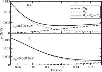
Figure 6: Temperature dependence of electrical conductivity for pion (dotted line), nucleon (dashed line) components and their total (solid line) at $\mu_{N}=0.500$ GeV (a) and $\mu_{N}=0.300$ GeV.

Figure 7: $\mu_{N}$ dependence of electrical conductivity for pion (dotted line), nucleon (dashed line) components and their total (solid line) at $T=0.120$ GeV (a) and $T=0.150$ GeV.

Using the $\Gamma_{\pi(\pi\sigma)}(\vec{k},T)$, $\Gamma_{\pi(\pi\rho)}(\vec{k},T)$ and their total in the integrand of Eq. (25), the dotted, dashed and solid lines of Fig. (3) are generated, where folding GKS by vacuum spectral functions of resonances $\sigma$ and $\rho$ are considered in panel (a) but not in panel (b). Like the results of shear viscosity in the earlier work GKS , $\sigma$ and $\rho$ resonances play dominant role in the electrical conductivity at low ($T<0.100$ GeV) and high ($T>0.100$ GeV) temperature domain respectively. We get $\sigma_{\pi}(T)$ as a decreasing function in low and high temperature both, although a mild increasing function of shear viscosity $\eta_{\pi}(T)$ has been observed in Ref. GKS at high temperature domain of hadronic matter ($0.100$ GeV $<T<0.175$ GeV). The mathematical origin for this differences in the nature of $\sigma_{\pi}(T)$ and $\eta_{\pi}(T)$ is because of different power of momentum ($\vec{k}^{4}$ for $\sigma_{\pi}$ but $\vec{k}^{6}$ for $\eta_{\pi}$) in the numerator of their respective integrand.

Adding baryonic loop contributions with the mesonic loops of pion self-energy, we get total thermal width of pion as described explicitly in Eq. (28). Fig. 4(a) and (b) for $\mu_{N}=0$ and $0.300$ GeV reveal that $\sigma_{\pi}(T)$ reduces after adding baryonic loop contribution in pion self-energy and its reduction strength becomes larger for larger values of $\mu_{N}$ as baryonic loop contribution, $\Gamma_{\pi(NB)}(\vec{k},T,\mu_{N})$ depends sensitively on $\mu_{N}$. To display the dominant contribution of $N\Delta$ loop ($\Gamma_{\pi(N\Delta)}$), Fig. (4) shows individual contributions of meson loops, meson loops + $N\Delta$ loop and meson + baryon loops by dotted, dashed and solid lines respectively.

Next, Fig. 4(a) and (b) for $T=0.120$ GeV and $0.150$ GeV show $\mu_{N}$ dependence of electrical conductivity of pionic component for meson loops (dotted line), meson loops + $N\Delta$ loop (dashed line) and meson + baryon loops (solid line). As $\Gamma_{\pi(\pi M)}(\vec{k},T)$ is independent of $\mu_{N}$, therefore corresponding $\sigma_{\pi}$ (dotted line) remain constant with the variation of $\mu_{N}$. After adding $N\Delta$ loop (dashed line) and other baryon loops (solid line), a decreasing nature of $\sigma_{\pi}(\mu_{N})$ are clearly noticed. A sensitive dependence of $\mu_{N}$ in $\Gamma_{\pi(NB)}$ for $N\Delta$ loop (dominant) and other baryon loops are the main reason behind the decreasing nature of $\sigma_{\pi}(\mu_{N})$.

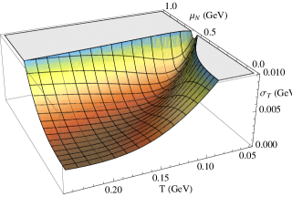
Figure 8: (Color online) Total electrical conductivity $\sigma_{T}$ in $T$-$\mu_{N}$ plane.

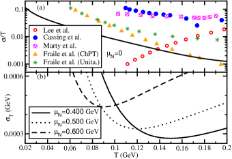
Figure 9: (Color online) Our results of $\sigma(T,\mu_{N}=0)/T$ are compared with the results of Refs. Cassing ; Marty ; Lee ; Nicola_PRD (a). Valley structure of $\sigma(T)$ at $\mu_{N}=0.400$ GeV, $0.500$ GeV, $0.600$ GeV are shown by solid, dotted and dashed lines respectively in panel (b).

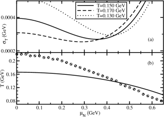
Figure 10: (a): Valley structure of $\sigma(\mu_{N})$ at three different $T$. (b): The points of minima (solid circles) and freeze out line freezeout (solid line) are shown in $T$-$\mu_{N}$ plane.

In Fig. 6(a) and (b) for $\mu_{N}=0.500$ GeV and $0.300$ GeV, the $T$ dependence of pionic ($\sigma_{\pi}$), nucleonic ($\sigma_{N}$) components of electrical conductivities and their total ($\sigma_{T}$) are shown by dotted, dashed and solid lines respectively. Corresponding results in $\mu_{N}$ axis are shown in Fig. 7(a) and (b) for $T=0.120$ GeV and $0.150$ GeV. Unlike to $\sigma_{\pi}$, the $\sigma_{N}$ increases with both $T$ and $\mu_{N}$. The nucleon phase space factors or statistical weight factors of FD distributions in $\sigma_{N}$ are playing a dominant over the $\Gamma_{N}(T,\mu_{N})$, whereas for pionic case, $\Gamma_{\pi}(T,\mu_{N})$ becomes more influential than pionic phase factors or statistical Bose enhanced weight factors in $\sigma_{\pi}$. This is the mathematical reason for opposite nature of $\sigma_{\pi}(T,\mu_{N})$ and $\sigma_{N}(T,\mu_{N})$. From a simultaneous observation of Fig. (6) and (7), we can conclude that the decreasing nature of $\sigma_{T}(T,\mu_{N})$ becomes inverse beyond a certain points of $T$ and $\mu_{N}$, where $\sigma_{T}$ exposes the points of minima. This behavior can be visualized well from Fig. (8), which exhibits 3-dimensional plot of $\sigma_{T}(T,\mu_{N})$.

Up to now, our results are presented as normalized values of $e^{2}$ (in other word we have taken $e^{2}=1$) but exact values of $\sigma_{T}$ (after multiplying by $e^{2}=4\pi/137$) have been shown in the last two figures (9) and (10). Fig. 9(a) displays a comparison of present results with the earlier results, obtained by Fraile et al. Nicola (stars and triangles), Lee et al. Lee (open circles), Marty et al. Marty (squares), Cassing et al. Cassing (solid circles) at hadronic temperature domain for $\mu_{N}=0$. Within $0.110$ GeV $<T<0.175$ GeV, present results more or less agrees with the results of Ref. Nicola ; Lee but quite smaller than the results of Ref. Marty ; Cassing . Fig. 9(b) shows $\sigma_{T}$ vs $T$ at three different values of $\mu_{N}$, where we notice the shifting of minimum values of $\sigma_{T}$ towards lower $T$ as one increases $\mu_{N}$. Alternatively, these minimum values of $\sigma_{T}$ will also be shifted towards lower $\mu_{N}$ as $T$ will increase, which is explicitly shown in Fig. 10(a). Next, Fig. 10(b) represents the points of minima for $\sigma_{T}$ in $T$-$\mu_{N}$ plane. An approximated freeze out line (solid line), taken from Ref. freezeout , is also pasted in Fig. 10(b). The points of minima, which are located outside the freeze out line, can only be covered by the expanding fireball, produced in different beam energies of heavy ion collisions. Therefore, the minima or valley structure can be observed from ($T_{f}\approx 0.166$ GeV, $\mu_{f}\approx 0$) to ($T_{f}\approx 0.140$ GeV, $\mu_{f}\approx 0.420$ GeV), where subscript $f$ stands for freeze out. In other word, from high beam energy $\sqrt{s}$ like RHIC experiment ($\sqrt{s}=200$ GeV), this valley structure can be observed up to $\sqrt{s}\approx 8$ GeV. However, within this long range of beam energy or freeze out line, some points of minima may cross the quark-hadron transition line and therefore, they may not be observed in the experiment. One should keep in mind that these minima or valley structure is completely appeared due to phase space effect of hadronic medium and has nothing relation with the quark-hadron transition. Therefore, one can observe only those points of minima of hadronic medium, which will be in between freeze out and quark-hadron transition lines. Although, there is some possibility for not observing any points of minima, if they all are located in quark phase domain of $T$-$\mu_{N}$ plane. In this regards, we can say at least that $\sigma(T,\mu_{N})$ of hadronic medium decreases as one goes towards quark-hadron transition line.

We have presented the numerical values of $\sigma(T,\mu_{N}=0)/T$, estimated by earlier works in Table 1, where most of the works are displaying the decreasing $\sigma(T)/T$ in hadronic temperature  Cassing ; Marty ; Nicola_PRD ; Nicola and increasing $\sigma(T)/T$ in temperature domain of quark phase Cassing ; Marty ; Puglisi ; Greif ; PKS ; Finazzo ; LQCD_Amato . Among them, Refs. Cassing ; Marty , covering the both temperature domain, have exhibited the minimum value of $\sigma/T$ near transition temperature. On the basis of these earlier results at $\mu_{N}=0$ and our estimations at finite $\mu_{N}$ within the $T$-$\mu_{N}$ domain of hadronic matter, a valley structure along quark-hadron transition line in $T$-$\mu_{N}$ plane may be expected and this issue may be confirmed after further research on $\sigma$-calculations at finite baryon density, based on different effective QCD model.

	$\sigma/T$ at	$\sigma/T$ at
	$T=(0.120$	$T=(0.175$
	-$~{}0.175)$ GeV	-$~{}350)$ GeV
LQCD Results:
Gupta LQCD_Gupta	-	$\approx 0.375$
Ding et al. LQCD_Ding	-	$\approx 0.033(+0.018,$
		$~{}~{}~{}~{}~{}~{}-0.016)$
Arts et al. LQCD_Arts_2007	-	$\approx 0.020(\pm 0.005)$
Brandt et al. LQCD_Barndt	-	$\approx 0.020(\pm 0.006)$
Burnier et al. LQCD_Burnier	-	$\approx 0.0064$
Amato et al. LQCD_Amato	-	$\approx 0.003(\pm 0.001)$
		-$~{}0.015(\pm 0.003)$
Buividovich et al. LQCD_Buividovich	-	$\approx 0.0021(\pm 0.0003)$
Yin Yin	-	$\approx 0.06(+0.04,$
		$-0.02)$
Puglisi et al. Puglisi	-	$\approx 0.09~{}$-$~{}0.13$
(PQCD in RTA)
Puglisi et al. Puglisi	-	$\approx 0.01~{}$-$~{}0.07$
(QP in RTA)
Greif et al. Greif	-	$\approx 0.04~{}$-$~{}0.06$
(BAMPS)
Marty et al. Marty	-	$\approx 0.06~{}$-$~{}0.16$
(DQPM)
Marty et al. Marty	$\approx 0.06~{}$-$~{}0.05$	$\approx 0.05~{}$-$~{}0.5$
(NJL)
Cassing et al. Cassing	$\approx 0.088~{}$-$~{}0.025$	$\approx 0.025~{}$-$~{}0.2$
(PHSD)
Finazzo et al. Finazzo	$\approx 0.004~{}$-$~{}0.010$	$\approx 0.010~{}$-$~{}0.015$
Lee et al. Lee	$\approx 0.001~{}$-$~{}0.011$	$\approx 0.36~{}$-$~{}0.015$
Fraile et al. Nicola	$\approx 0.013~{}$-$~{}0.010$	-
(Unitarization)
Fraile et al. Nicola	$\approx 0.008~{}$-$~{}0.002$	-
(ChPT)
Present Results	$\approx 0.004~{}$-$~{}0.001$	-

Table 1: At $\mu_{N}=0$, the $\sigma(T)/T$ in approximated temperature domain of hadronic ($T\approx 0.120$ GeV to $0.175$ GeV) and quark ($T\approx 0.175$ GeV to $0.350$ GeV) phases are presented in 2nd and 3rd columns, whereas in 1st column, the references (with their methodologies) are addressed.

V Summary and Conclusion

The present work provide an estimation of electrical conductivity of hadronic medium at finite temperature and baryon density. Assuming pion and nucleon as most abundant medium constituents, we have first deduced thermal correlators of their electromagnetic currents and then, taking the static limit of these correlators, the expressions of electrical conductivities for pionic and nucleonic components are derived. For getting the non divergent values of these correlators in the static limit, one has to include the finite thermal widths of the medium constituents - pion and nucleon. This is a traditional quasi-particle technique of Kubo frame work, used during the calculations of transport coefficients from the relevant correlators in their static limits. Following the field theoretical version of optical theorem, the thermal widths of pion and nucleon are obtained from the imaginary part of their one-loop self-energy diagrams, which accommodate different mesonic and baryonic resonances in the intermediate states. As a dynamical part, the interaction of pion and nucleon with other mesonic and baryonic resonances are guided by the effective hadronic Lagrangian densities, where their couplings are tuned by the decay width of resonances, based on the experimental data from PDG. The momentum distribution of these thermal widths are integrated out during evaluation of electrical conductivities of respective components.

The electrical conductivity for pionic component is obtained as a decreasing function $T$ and $\mu_{N}$, where mesonic loops are dominant to fix its numerical strength. The $\pi\sigma$ and $\pi\rho$ loops of pion self-energy control the strength of electrical conductivity at low and high $T$ regions respectively. While a further reduction of numerical values in conductivity at high $T$ domain is noticed after addition of different baryonic loops in pion self-energy. Electrical conductivity of pionic component due to mesonic loops remain constant with $\mu_{N}$ but it is transformed to a decreasing function when the baryonic loops are added in the pion self-energy. The nucleonic component give the increasing values of electrical conductivity with the variation of $T$ and $\mu_{N}$. After adding these pionic and nucleonic components, the total electrical conductivity first decreases at pion dominating $T$-$\mu_{N}$ domain and then increases at nucleonic dominating domain. Therefore, the numerical results show a set of $T$-$\mu_{N}$ points, where total electrical conductivity becomes minimum and this valley structure in $T$-$\mu_{N}$ plane can only be observed if the points of minima are located between freeze out line and quark-hadronic transition line.

Comparing with earlier estimations of electrical conductivity at $\mu_{N}=0$, present work more or less agrees with Refs. Nicola ; Lee quantitatively and quantitatively it is similar with most of the earlier works Cassing ; Marty ; Nicola_PRD ; Nicola ; Greif2 , which show that electrical conductivity at $\mu_{N}=0$ decreases with $T$. On the basis of these earlier studies at $\mu_{N}=0$ and present investigation at finite $\mu_{N}$, a general decreasing nature in the numerical values of electrical conductivity for hadronic matter is observed when one goes from freeze out to quark-hadron transition line in $T$-$\mu_{N}$ plane. Further research in different model calculations at finite $\mu_{N}$ may confirm this conclusion.

Acknowledgment : The work is financially supported from UGC Dr. D. S. Kothari Post Doctoral Fellowship under grant No. F.4-2/2006 (BSR)/PH/15-16/0060.

VI Appendices

VI.1 Calculation $N(\vec{q},\vec{k})$

Let us write the 11-component of two point function of current-current correlator in terms of field operators. For $\phi_{\pi}$ field it is given by

$$\Pi_{11}(q) = i\int d^{4}xe^{iqx}\langle TJ^{\rm EM}_{\mu}(x)J_{\rm EM}^{\mu}(0)\rangle_{\beta}$$

$$= ie^{2}\int d^{4}xe^{iqx}\langle T\phi_{\pi}(x)\partial_{\mu}\phi_{\pi}(x)\phi_{\pi}(0)\partial^{\mu}\phi_{\pi}(0)\rangle_{\beta}~{}.$$

With the help of the Wick’s contraction technique, we have

$$\Pi_{11}(q) = ie^{2}\int d^{4}xe^{iqx}[\langle T\phi_{\pi}\underbrace{(x)\partial_{\mu}\phi_{\pi}\overbrace{(x)\phi_{\pi}}(0)\partial^{\mu}\phi_{\pi}}(0)\rangle_{\beta}$$

$$= ie^{2}\int\frac{d^{4}k}{(2\pi)^{4}}N(q,k)D_{11}(k)D_{11}(p=q-k)~{},$$

where

$$N(q,k)=(-4)k^{\mu}(q-k)_{\mu}$$ (42)

and its space component part is

$$N(\vec{q},\vec{k})=(-4)\{-\vec{k}\cdot\vec{q}+\vec{k}^{2}\}~{}.$$ (43)

Similarly for $\psi_{N}$ field,

$$\Pi_{11}(q) = ie^{2}\int d^{4}xe^{iqx}\langle T{\overline{\psi}}_{N}\underbrace{(x)\gamma_{\mu}\psi_{N}\overbrace{(x){\overline{\psi}}_{N}}(0)\gamma^{\mu}\psi_{N}}(0)\rangle_{\beta}$$

$$= ie^{2}\int\frac{d^{4}k}{(2\pi)^{4}}N(q,k)D_{11}(k)D_{11}(p=q+k)~{},$$

where

$$N(q,k) = {\rm Tr}[\gamma^{\mu}(q\!\!\!/+k\!\!\!/+m_{\psi})\gamma_{\mu}(k\!\!\!/+m_{\psi})]$$ (45)

$$= 8k^{\mu}(q+k)_{\mu}-4[k\cdot(q+k)-m_{\psi}^{2}]g^{\mu}_{\mu}$$

and the space component part of

$$N(q,k_{0}=\pm\omega_{k},\vec{k})=8k^{\mu}(q+k)_{\mu}-4[k\cdot q]g^{\mu}_{\mu}$$ (46)

is

$$N(\vec{q},\vec{k})=-8\vec{k}\cdot(\vec{q}+\vec{k})+4[\vec{k}\cdot\vec{q}]g^{i}_{i}~{}.$$ (47)

VI.2 Application of L’Hospital rule

For finite value of $\Gamma$, the Eq. (LABEL:el_G) becomes

$$\sigma=\frac{e^{2}}{3}\int\frac{d^{3}k}{(2\pi)^{3}}\frac{N^{0}}{4\omega_{k}^{2}\Gamma}\lim_{q_{0},\vec{q}\rightarrow 0}\left[\frac{C_{2}}{q_{0}}+\frac{C_{3}}{q_{0}}\right]~{},$$ (48)

as

$$\lim_{\vec{q}\rightarrow 0}\omega_{p}=\omega_{k}~{}.$$ (49)

Applying L’Hospital’s rule, we can write

$$\lim_{q_{0}\rightarrow 0}\frac{C_{2,3}(q_{0})}{q_{0}} = \lim_{q_{0}\rightarrow 0}\frac{\frac{d}{dq_{0}}\{C_{2,3}(q_{0})\}}{\frac{d}{dq_{0}}\{q_{0}\}}$$ (50)

$$= \frac{d}{dq_{0}}\{\pm n^{\mp}_{p}(\omega_{p}=\mp q_{0}+\omega_{k})\}$$

$$= \beta[n^{\mp}_{k}(1+\epsilon_{k}n^{\mp}_{k})]~{},$$

since

$$\left(\pm\right)\frac{d}{dq_{0}}n^{\mp}_{p}(\omega_{p}=\mp q_{0}+\omega_{k}) = \left(\pm\right)\frac{-\beta\frac{d\omega_{p}}{dq_{0}}e^{\beta(\omega_{p}\pm\mu)}}{\{e^{\beta(\omega_{p}\pm\mu)}+\epsilon_{k}\}^{2}}$$

$$\lim_{q_{0}\rightarrow 0}\left(\pm\right)\frac{d}{dq_{0}}n^{\mp}_{p}(\omega_{p}=\mp q_{0}+\omega_{k}) = \left(\pm\right)\frac{-\beta\left(\mp\right)e^{\beta(\omega_{k}\pm\mu)}}{\{e^{\beta(\omega_{k}\pm\mu)}+\epsilon_{k}\}^{2}}$$

$$= \beta[n^{\mp}_{k}(1+\epsilon_{k}n^{\mp}_{k})]~{}.$$

References

- (1) R. Rapp Adv. High Energy Phys. 2013, 148253 (2013); R. Rapp, J. Wambach 2000 Adv. Nucl. Phys. 25, 1 (2000).
- (2) P. Mohanty, S. Ghosh, S. Mitra Adv. High Energy Phys. 2013, 176578 (2013).
- (3) R. Arnaldi et al. (for the NA60 collaboration) Phys. Rev. Lett. 100, 022302 (2008); R. Arnaldi et al. (for the NA60 collaboration) Eur. Phys. J. C 61, 711 (2009); S. Damjanovic et al. (for the NA60 Collaboration) J. Phys. G: Nucl. Part. Phys. 35, 104036 (2008).
- (4) E. Braaten and R.D. Pisarski, Nucl. Phys. B 337, 569 (1990).
- (5) C.A. Islam, S. Majumder, N. Haque, M.G. Mustafa, J. High Energy Phys. 1502 (2015) 011.
- (6) A. Bzdak, V. Skokov, Phys. Lett. B 710 (2012) 171.
- (7) K. Tuchin, Adv. High Energy Phys. 2013, 490495 (2013).
- (8) Y. Akamatsu, H. Hamagaki, T. Hatsuda, T Hirano, J. Phys. G 38 (2011) 124184
- (9) Y. Yin, Phys. Rev. C 90, 044903 (2014).
- (10) Y. Hirono, M. Hongo, T. Hirano Phys. Rev. C 90, 021903 (2014).
- (11) W. Cassing, O. Linnyk, T. Steinert, and V. Ozvenchuk, Phys. Rev. Lett. 110, 182301 (2013).
- (12) R. Marty, E. Bratkovskaya, W. Cassing, J. Aichelin, H. Berrehrah, Phys. Rev. C 88 (2013) 045204.
- (13) A. Puglisi, S. Plumari, V. Greco, Phys. Rev. D 90, 114009 (2014); J. Phys. Conf. Ser. 612 (2015) 012057; Phys. Lett. B 751 (2015) 326.
- (14) M. Greif, I. Bouras, Z. Xu, C. Greiner, Phys. Rev. D 90 (2014) 094014; J. Phys. Conf. Ser. 612 (2015) 012056.
- (15) P. K. Srivastava, L. Thakur, B. K. Patra, Phys. Rev. C 91, 044903 (2015).
- (16) S. I. Finazzo, J. Noronha Phys. Rev. D 89, 106008 (2014).
- (17) C. Lee, I. Zahed, Phys. Rev. C 90, 025204 (2014).
- (18) D. Fernandez-Fraile and A. Gomez Nicola, Phys. Rev. D 73, 045025 (2006).
- (19) D. Fernandez-Fraile and A. Gomez Nicola, Eur. Phys. J. C 62, 37 (2009).
- (20) M. Greif, C. Greiner, G.S. Denicol, Phys. Rev. D 93, 096012 (2016).
- (21) H.T. Ding, A. Francis, O. Kaczmarek, F. Karsch, E. Laermann, and W. Soeldner, Phys. Rev. D 83, 034504 (2011).
- (22) G. Aarts, C. Allton, J. Foley, S. Hands, and S. Kim, Phys. Rev. Lett. 99, 022002 (2007).
- (23) P. V. Buividovich, M. N. Chernodub, D. E. Kharzeev, T. Kalaydzhyan, E. V. Luschevskaya, and M. I. Polikarpov, Phys. Rev. Lett. 105, 132001 (2010).
- (24) Y. Burnier and M. Laine, Eur. Phys. J. C 72, 1902 (2012).
- (25) S. Gupta, Phys. Lett. B 597, 57 (2004).
- (26) B. B. Brandt, A. Francis, H. B. Meyer, and H. Wittig, J. High Energy Phys. 03 (2013) 100.
- (27) A. Amato, G. Aarts, C. Allton, P. Giudice, S. Hands, J.I. Skullerud, Phys. Rev. Lett. 111, 172001 (2013).
- (28) D. N. Zubarev Non-equilibrium statistical thermodynamics (New York, Consultants Bureau, 1974).
- (29) R. Kubo, J. Phys. Soc. Jpn. 12, 570 (1957).
- (30) S. Ghosh, Int. J. Mod. Phys. A 29 (2014) 1450054.
- (31) S. Ghosh, G. Krein, S. Sarkar, Phys. Rev. C 89 (2014) 045201.
- (32) S. Ghosh, J. Phy. G 41, 095102 (2014).
- (33) S. Ghosh, Braz. J. Phys. 45 (2015) 6, 687.
- (34) M. Post, S. Leupold, U. Mosel, Nucl. Phys. A 741, 81 (2004).
- (35) S. Ghosh, Phys. Rev. C 90, 025202 (2014).
- (36) S. Ghosh, Braz. J. Phys. 44, 789 (2014).
- (37) F. Karsch and K. Redlich, Phys. Lett. B 695, 136 (2011).