Structure function and fractal dissipation for an intermittent inviscid dyadic model

Abstract

We study a generalization of the original tree-indexed dyadic model by Katz and Pavlović for the turbulent energy cascade of three-dimensional Euler equation. We allow the coefficients to vary with some restrictions, thus giving the model a realistic spatial intermittency. By introducing a forcing term on the first component, the fixed point of the dynamics is well defined and some explicit computations allow to prove the rich multifractal structure of the solution. In particular the exponent of the structure function is concave in accordance with other theoretical and experimental models. Moreover anomalous energy dissipation happens in a fractal set of dimension strictly less than 3.

1 Introduction

Three dimensional turbulent fluids are far from being fully understood, from a mathematical point of view. Even if we know the equations governing the behaviour of the fluid, extracting the laws of turbulence is extremely difficult. It is not surprising, then, that many simplified models have been developed in the past years to capture at least some aspects of turbulent fluids. Among those the shell models are of particular interest. Introduced by Novikov, they have many variants. We recall here the dyadic model [26] and the GOY, as introduced by Gledzer [34] and Ohkitani and Yamada [46].

The study of shell models in turbulence is well established in the physics literature, in particular for the relative ease of numerical simulation. A nice review of this is Biferale [18].

The model we are interested in belongs to the family of dyadic shell models, and was introduced by Katz and Pavlović [37]. Its main feature is the tree structure of the components, which allows to write a simplified wavelet description of the Euler equations. (Conversely, the more common integer-indexed shell models are constructed to be reminiscent of Littlewood-Paley decomposition.)

Even if the motivations for these models are quite different, it is also natural to see the tree models as generalizations of the usual shell models. This has been done for example by Benzi and Biferale for the GOY model in [15] and in [4] for many results that were proved about the dyadic in [6].

Anomalous dissipation.

One of the main features of most inviscid shell models is the blow-up of regularity, linked to the “anomalous” dissipation of energy. With the latter we intend that the non-linear, formally conservative term, “fires” lumps of energy to smaller and smaller scales, making them actually disappear. In passing from Euler to Navier-Stokes, the introduction of a term corresponding to the viscosity of the fluid may sometimes be enough to brake this phenomenon (as was proved for the dyadic model with viscosity in [8]), but the non-linear term can be tailored to overcome thermal dissipation, in fact Tao in [54] used a shell model to prove that some averaged versions of three-dimensional Navier-Stokes equation have blow-up.

Anomalous dissipation is connected to Onsager’s conjecture on the regularity of the solutions of Euler equation, discussed later on.

RCM, tree dyadic with repeated coefficients.

In this paper, we build on the previous work in [4], and consider a more general model, that still exhibits anomalous dissipation of energy. The model will be introduced in the following section. The main difference from the literature is that we allow the coefficients of the non-linear term to depend on the nodes of the tree not only through their generation. Every node $j$ of the tree has $N=2^{d}=8$ children $j_{1},j_{2},\dots,j_{N}$ and interacts with each one of them in the same way but for a coefficient $c_{j_{i}}=2^{\alpha|j|}\delta_{i}$, where $\{\delta_{1},\dots,\delta_{N}\}$ are fixed positive numbers that are repeated for all nodes $j$ and $|j|$ is the generation of $j$. We call this the model with repeated coefficients or RCM.

In the previous models from the literature the choice was $\delta_{i}\equiv 1$, and in many cases the solutions were uniform in phase space and quite regular in physical space. Allowing for different $\delta_{i}$’s forces spatial intermittency on the solutions, thus yielding interesting results in terms of structure function and singularities spectrum. From a physical point of view, we see this generalization as a picture of the “istantaneous” Euler dynamics, as explained in Remark 1.

Structure function.

Structure functions are among the main objects studied in physics to give a statistical description of the energy cascade in turbulence. These are denoted by $S_{p}(r)$ and defined as the $p$-moments of the velocity increments on the scale $r$. In his cornerstone work on the theory of turbulence K41 [38], Kolmogorov postulated that $S_{p}(r)\sim r^{p/3}$, but subsequent numerical and experimental studies (for example [2, 11, 12, 40]) did not fully agree with such prediction, showing instead a scaling exponent nonlinearly dependent on $p$: $S_{p}(r)\sim r^{\zeta_{p}}$. This discrepancy is evidence of a multifractal spectrum of the singularities and is usually attributed to some spatial intermittency of the energy cascade (see [16, 49, 42, 51] and many references therein).

To cope with this discrepancy, in the past years there have been several attempts to develop phenomenological models for the energy cascade which are intermittent and self-similar. To cite just a few, there is the log-normal model by Kolmogorov and Obukhov [39, 45], the random curdling by Mandelbrot [41], the $\beta$-model by Frisch, Sulem and Nelkin [33], the random $\beta$-model by Benzi, Paladin, Parisi and Vulpiani [16], to the more recent $\alpha$- and $p$-models (see [42] for an excellent review) and finally, the log-Poisson model by She and Lévêque [52].

Many of these models actually exhibit a concave $\zeta_{p}$, thus yielding rich multifractal structure, but none are obtained as solutions of a dynamical model. On the other hand, Benzi, Biferale and Parisi in [14] deduce a plausible $\zeta_{p}$ for the stationary distribution of the GOY shell model, but their derivation is not rigorous.

One of the main results of this paper is that the constant solution of RCM is a self-similar, multifractal function that truly exhibits a non-linear scaling exponent of singularities, with a concave graph not dissimilar from those coming from numerical experiments. (On the contrary, the dyadic shell model and the tree dyadic model both agree with Kolmogorov theory and have $\zeta_{p}=p/3$.)

As already stated, this is linked to spatial intermittency of the energy cascade. Truly, one can introduce the measure associated with turbulent energy cascade of the solution, and prove that this measure is itself a self-similar, multifractal, multiplicative cascade.

Onsager conjecture.

In [48], while trying to understand the phenomenon of energy dissipation in three-dimensional turbulent fluids for vanishing viscosity, Lars Onsager stated the conjecture that bears his name: that solutions of the incompressible Euler equations are energy preserving if they have a Hölder regularity greater than $1/3$ and that for every Hölder exponent $\alpha\leq 1/3$ there exists a weak solution of the Euler equation in $C^{\alpha}$ that dissipates energy.

The first half of this conjecture has been proven by Constantin, E and Titi [24] for three-dimensional Euler equations, in the setting of Besov spaces, building on a previous work by Eyink [29]. The second half lead to the development of many partial results, in particular by Buckmaster, De Lellis, Isett and Székelyhidi [20, 19, 35], but it is still open.

It is worth noting that the unique constant solution of our model always exhibits anomalous dissipation and it has Hölder regularity $h\leq 1/3$. In particular $h<1/3$ if the coefficients $\delta_{i}$ are not all equal. (See Theorem 4.1.) This is in accordance with Onsager’s conjecture. Moreover, if we introduce the local Hölder exponent $s(x)$ for each point $x$, then $s(x)\geq h$ and it is possible to compute its multifractal spectrum and to show that anomalous dissipation occurs at all points $x$ for which $s(x)\leq 1/3$.

Constant solutions.

One serious drawback of RCM is that it is mathematically hard to deal with. In fact we cannot prove significant results for the general solution of the problem. Instead we introduce a constant forcing term on the first component and look for constant solutions.

The fact that finite-energy, constant solutions exist, is per se an interesting proof of anomalous dissipation, but —what is more important— the constant solution can be made completely explicit, and its structure analysed in every detail.

One might wonder if considering only constant solutions is too restrictive, but we stress that they are an interesting first step that motivates further study of models on trees with variable coefficients. Moreover it is reasonable to conjecture that the constant solution is an attractor (as is the case for the dyadic shell model, see Cheskidov et al. [23]), making its properties even more interesting. The next natural step would be to study solutions that are not constant in time but statistically stationary, in some sense. We believe that many properties of constant solutions are universal and hence would hold also for stationary solutions.

Main results.

For the sake of clarity, we state here the main results of the paper in the physically meaningful case, that is $d=3$ and $\alpha=5/2$. The complete statements and the proofs can be found in Section 3, 4 and 5.

Theorem 1.1.

There exists a unique constant finite-energy solution for the RCM. The exponents of the structure function corresponding to this solution are given by

$$\zeta_{p}=\frac{p}{3}+\frac{p}{2}(\ell_{3/2}-\ell_{p/2}),\qquad p\geq 0$$

where $\ell_{s}$ is a function of $s$ that depends on the repeated coefficients $\delta_{i}$’s: it is constant if they are all equal, while otherwise it is strictly increasing with finite limits at $\pm\infty$. In the latter case, the function $\zeta_{p}$ is strictly concave and has an oblique asymptote. Moreover if the ratio between the maximum of $\delta_{i}^{3/2}$, $i=1,2,\dots,N$ and their average is less then 2, then $\zeta_{p}$ is increasing for all $p$.

This depicts a model with spatial intermittency, as the scaling exponents, for $p>3$, lie below the Kolmogorov’s $p/3$ line.

To study the geometry of anomalous dissipation we associate each index $j\in J$ to one cube $Q_{j}$ of side $2^{-|j|}$ in the dyadic lattice $\bigcup_{n}(2^{-n}[0,1])^{3}$ and identify a non-negative term $F_{j}$ measuring the energy dissipated inside the cube $Q_{j}$, with the property that

$$\sum_{|j|=n}F_{j}=1.$$

Theorem 1.2.

Suppose the repeated coefficients $\delta_{i}$’s are not all equal. Then there is a set $\mathcal{H}\subset[0,1]^{3}$ of Hausdorff dimension strictly less than 3 such that

$$\sum_{\begin{subarray}{c}|j|=n\\ Q_{j}\cap\mathcal{H}\neq\emptyset\end{subarray}}F_{j}=1,\qquad\sum_{\begin{subarray}{c}|j|=n\\ Q_{j}\cap\mathcal{H}=\emptyset\end{subarray}}F_{j}=0,\qquad n\geq 1$$

and

$$\lim_{n\to\infty}\operatorname{Vol}\biggl{(}\bigcup_{\begin{subarray}{c}|j|=n\\ Q_{j}\cap\mathcal{H}\neq\emptyset\end{subarray}}Q_{j}\biggr{)}=0.$$

The structure of the paper is the following: in Section 2 we introduce our model and discuss its physical meaning, with some additional details presented in Appendix A. In Section 3 we prove existence and uniqueness of the constant solution, then we move on to determine the form of the exponent in the structure function and discuss its properties in Section 4. Finally, in Section 5, we prove the multifractality results for the anomalous dissipation of energy.

2 The models

This section is devoted to the presentation of the dyadic tree model introduced by Katz and Pavlović in [37] and studied again in Barbato et al. [4] and to its generalization, which is the main model of this paper.

These models specify the dynamics in terms of some coefficients $(v_{j}(t))_{j}$, indexed by a tree $J$. The equations have some likeness to those one would get with any wavelet decomposition of Euler equations:

$$\frac{d}{dt}v_{j}(t)=\sum_{k,l\in J}C_{j,k,l}v_{k}(t)v_{l}(t).$$

In the previous works the model has been studied as an abstract formulation, but in the present work we would like to investigate also some geometric properties of the physical “solution”, in the physical space.

To this end, we prove rigorous statements for the abstract model, but give also non-rigorous consequences for a physical “solution” which we imagine to be recomposed from the coefficients $v_{j}(t)$’s through any orthonormal family $(\psi_{j}(x))_{j}$ of wavelets on a cube $Q_{\emptyset}$ of ${\mathbb{R}}^{d}$.

$$v(t,x)\coloneqq\sum_{j\in J}v_{j}(t)\psi_{j}(x),\qquad t\geq 0,x\in Q_{\emptyset}.$$ (1)

We do not explicitly choose the wavelets, but try to deduce universal consequences, which would not depend on the choice. In particular, for our purposes, the physical “solution” $v(t)$ will be a scalar field whose regularity is what we propose to study.

Consider a solution which is stationary in some sense, $v(t,x)\approx u(x)$ for all $t$. The structure function of order $p$ of $u$ is defined by

$$S_{p}(r)\coloneqq\int_{Q_{\emptyset}}\left\langle|u(x)-u(y)|^{p}\right\rangle_{y}dx$$

where $\langle\cdot\rangle_{y}$ denotes the average on the points $y$ such that $|y-x|=r$.

This is a very popular tool to study turbulence in fluid mechanics. In particular one often considers the infinitesimal behaviour of $S_{p}(r)$ as $r\to 0$, introducing the exponents of the structure function, that is

$$\zeta_{p}\coloneqq-\lim_{n\to\infty}\frac{1}{n}\log_{2}S_{p}(2^{-n}).$$ (2)

It is known that $\zeta_{p}$ is linked to the Besov norms $B_{p}^{s,\infty}$, which in turn can be computed from the wavelet coefficients of $u$ in an universal fashion, not depending on the actual wavelet basis chosen.

In this section, after an introduction of the abstract model, we will link it to a physical solution, define and compute some Besov norms of the latter and finally deduce the formula of $\zeta_{p}$ in terms of the solution to the abstract model.

2.1 Abstract model

Let $d$ be the space dimension and let $N=2^{d}$. Consider the following set with its natural tree structure:

$$J\coloneqq\bigcup_{n=0}^{\infty}\{1,2,\dots,N\}^{n}=\{\emptyset,1,2,\dots,N,(1,1),(1,2),\dots\}.$$

For all $j=(j^{1},j^{2},\dots,j^{m}),k=(k^{1},k^{2},\dots,k^{n})\in J$, we define the append operator $jk\coloneqq(j^{1}\dots,j^{m},k^{1},\dots,k^{n})\in J$, the size operator $|j|\coloneqq m\in{\mathbb{N}}$, the partial ordering $j\leq k$ if and only if $k=jh$ for some $h\in J$ (with $j<k$ if moreover $|h|>0$), the father operator $\bar{\jmath}\in J$ such that $\bar{\jmath}<j$ and $|\bar{\jmath}|=|j|-1$ and the offspring set of $j$, $\mathcal{O}_{j}\coloneqq\{k\in J:\bar{k}=j\}$.

Our model is given by the following equations

$$v_{j}^{\prime}(t)=c_{j}v_{\bar{\jmath}}^{2}(t)-\sum_{k\in\mathcal{O}_{j}}c_{k}v_{j}(t)v_{k}(t),\qquad j\in J,\quad t\geq 0$$ (3)

where $c_{j}=d_{j}2^{\alpha|j|}$, $\alpha>0$, $d_{j}>0$ for $j\in J$, $d_{\emptyset}=1$ and $v_{\bar{\emptyset}}(t)\equiv f$.

It generalizes the model introduced by Katz and Pavlović in [37], where $f=0$ and $d_{j}=1$ for all $j\in J$.

The parameter $\alpha$ is left free in all statements, but from a physical point of view, some heuristic arguments based on Euler dynamics suggest to fix $\alpha=\frac{d}{2}+1$, which is what the other authors also used. See for example works by Katz, Pavlović, Friedlander and Cheskidov [37, 31, 22, 21]. Recently it was proved rigorously in Barbato et al. [9] that $\alpha\leq\frac{5}{2}$ for a Littlewood-Paley decomposition of the true three-dimensional Euler dynamics.

The generalization to variable $d_{j}$’s is very important. As we will see it completely changes the behaviour of anomalous dissipation and makes the function $\zeta_{p}$ strictly concave (as it should be, according to the most important numerical simulations of realistic turbulence models).

Remark 1.

We believe this generalization to be well justified from a physical point of view. When passing from a detailed description of Euler equations to any shell model of turbulence, many components (either Fourier or wavelets) are merged inside any single component of the shell model, thus the nonlinear interaction between adjacent shell components cannot be known precisely, and actually it depends on how the energy of the shell is distributed among the original components. In [9] for example a shell model is rigorously deduced from Euler equations and truly the coefficients $\varphi_{l,m,n}(t)$ of the nonlinear interaction turn out to be complicated, to depend on time and on the solution itself and they only allow to be studied by the bound $|\varphi_{l,m,n}(t)|\leq 2^{(5/2)\min(l,m,n)}$. This means that at any fixed time $t$ the true Euler dynamics, seen through a realistic shell model, have “instantaneous” coefficients of interactions which are all different and only statistically behave like $2^{(5/2)n}$.

In this sense looking for constant solutions of the models with variable coefficients identifies a very large class of fields among which we expect to find the solutions of the true Euler equations which in some sense are stationary or stable with respect to time evolution.

It would be really important to have a complete generality of the variable coefficients. In our model we always consider $|\log d_{j}|$ bounded and the more general results are proved in this setting. Nevertheless explicit computation of many quantities is possible only in the special case that the same fixed $N$ coefficients $\delta_{\omega}$ appear in every set of the form $\{d_{k}:k\in\mathcal{O}_{j}\}$. We call this the model with repeated coefficients or RCM (see Definition 3) and our most interesting and meaningful results are restricted to this model.

2.2 Physical space

Three-dimensional Navier-Stokes equations have been studied several times by means of multiresolution analysis or wavelet decomposition (see [25, 53] and references therein). The typical expression for the velocity field is

$$v(x,t)=\sum_{Q\in\mathcal{Q}}\sum_{a\in\mathcal{A}}v_{Q}^{a}(t)\psi_{Q}^{a}(x),$$

where $\mathcal{Q}$ is the set of the dyadic cubes inside $Q_{\emptyset}\coloneqq[0,1]^{3}$, $\psi_{Q}^{a}$ is a rescaling essentially supported on $Q$ of the “mother” $\psi_{Q_{\emptyset}}^{a}$ of the wavelets, and $\mathcal{A}$ is a fixed, finite set of indices that allow these wavelets to be a basis of some suitable functional space on $Q_{\emptyset}$. For example, to get a basis of $L^{2}({\mathbb{R}}^{3},{\mathbb{R}}^{3})$, one must provide 21 different “mother” wavelets (7 for each component) and the same number is required for divergence-free vector fields.

In the dyadic models of turbulence the phase-space $\mathcal{Q}\times\mathcal{A}$ is simplified to $\mathcal{Q}$ (in the case of [37] or our dyadic model on a tree [4, 17]) or even a quotient of $\mathcal{Q}$ (in classical shell models of turbulence that follow Littlewood-Paley decomposition). The non-linear interaction is constructed anew to be elementary but retain some of the main properties of the bilinear term in Euler equations.

In the present work in particular we identify $\mathcal{Q}$ with the tree $J$ through an isomorphism for which the relation $\subseteq$ on $\mathcal{Q}$ corresponds to $\geq$ on $J$.

More precisely, let $Q_{\emptyset}$ be the unit cube of ${\mathbb{R}}^{d}$, which is divided into $N=2^{d}$ cubes of side $\frac{1}{2}$ which are labelled $Q_{1},Q_{2},\dots,Q_{N}$ in some fixed way.

To each $j\in J$ we associate one cube $Q_{j}$ of side $2^{-|j|}$. Above we defined $Q_{j}$ for $|j|=0,1$. Then recursively, each cube $Q_{j}$ is divided into $N$ cubes of half side labelled $Q_{j1},\dots,Q_{jN}$ following the same ordering as for $j=\emptyset$ in such a way that for all $j,k\in J$ the homothety that maps $Q_{\emptyset}$ to $Q_{j}$ also maps $Q_{k}$ to $Q_{jk}$.

Then for a.e. point $x\in Q_{\emptyset}$ it is well defined the sequence $\emptyset=x_{0}<x_{1}<x_{2}<\dots$ of elements of $J$ such that $|x_{n}|=n$ and $x\in Q_{x_{n}}$, and we will identify $x$ with $(x_{n})_{n\geq 0}$ when convenient.

Consider a real function $\psi_{\emptyset}$ on $Q_{\emptyset}$, the “mother” of the wavelets and for all $j\in J$, let $\psi_{j}(x)\coloneqq 2^{d|j|/2}\psi_{\emptyset}(2^{|j|}x+\theta_{j})$, where $\theta_{j}$ is such that $\psi_{j}$ is supported on $Q_{j}$, the rescaling being the correct one to have all $\psi_{j}$’s with the same $L^{2}$-norm.

Given this family of wavelets, we can associate a real function $v(t,x)$ on $Q_{\emptyset}$ to any solution $(v_{j}(t))_{j}$ of the abstract model (3) through equation (1).

The regularity in space of the field $v(t,\cdot)$ can be studied by introducing suitable norms on the set of functions from $J$ to ${\mathbb{R}}$. In particular, given $u:J\to{\mathbb{R}}$, $p\in[1,\infty]$ and $s\in{\mathbb{R}}$, define a sequence $(\varepsilon_{n})_{n\geq 0}$ by

$$\varepsilon_{n}\coloneqq\begin{cases}2^{ns}2^{dn(\frac{1}{2}-\frac{1}{p})}\Bigl{(}\sum_{|j|=n}|u_{j}|^{p}\Bigr{)}^{1/p}&p<\infty\\ 2^{ns}2^{dn/2}\max_{|j|=n}|u_{j}|&p=\infty.\end{cases}$$

Then (see Meyer [43])

$$\sum_{j\in J}u_{j}\psi_{j}\in B_{p}^{s,q},\qquad\textup{if and only if}\qquad\varepsilon\in l^{q}({\mathbb{N}}).$$ (4)

With this identification of the Besov spaces at hand, we formally introduce the spaces corresponding to the usual function spaces $H^{s}$, $W^{s,p}$ and $C^{s}$ for sequences of real numbers indexed by $J$.

Definition 1.

For all $s\in{\mathbb{R}}$ we introduce the space $H^{s}$ of the maps $u:J\to{\mathbb{R}}$ such that the norm

$$\|u\|_{H^{s}}\coloneqq\Bigl{(}\sum_{j\in J}2^{2s|j|}u_{j}^{2}\Bigr{)}^{1/2}$$

is finite. In particular let $H\coloneqq H^{0}=l^{2}(J)$.

Moreover, for all $s\in{\mathbb{R}}$ and $p\geq 1$ we introduce the space $W^{s,p}$ of the maps $u:J\to{\mathbb{R}}$ such that the norm

$$\|u\|_{W^{s,p}}\coloneqq\Bigl{(}\sum_{j\in J}2^{ps|j|}2^{d(\frac{p}{2}-1)|j|}|u_{j}|^{p}\Bigr{)}^{1/p}$$

is finite. In particular $W^{s,2}=H^{s}$.

Finally, for all $s\in(0,1)$ we introduce the space $C^{s}$ of the maps $u:J\to{\mathbb{R}}$ such that

$$\sup_{n\geq 1}\biggl{(}ns+\frac{1}{2}dn+\max_{|j|=n}\log_{2}|u_{j}|\biggr{)}$$

is finite.

By condition (4), these spaces correspond to the usual ones for the recomposed function $\sum_{j\in J}u_{j}\psi_{j}$.

To make explicit the link between Besov norms and the exponents of the structure function, we refer to the works by Eyink [30] and by Perrier and Basdevant [50]. In the latter it is proven that if $\zeta_{p}$ is defined as usual by (2), then

$$\zeta_{p}=\sup\{s<p:u\in B_{p}^{s/p,\infty}\}.$$

Thus if $u(x)=\sum_{j\in J}u_{j}\psi_{j}(x)$, by condition (4),

$$\zeta_{p}=\min\biggl{\{}p;d-\frac{p}{2}d-\limsup_{n\to\infty}\frac{1}{n}\log_{2}\sum_{|j|=n}|u_{j}|^{p}\biggr{\}}.$$ (5)

In Appendix A we give some other argument, not fully rigorous, to show that this is indeed the correct exponent.

3 Well-posedness and regularity

In this section we will deal with the main model (3) in the abstract setting of the dyadic model on a tree. After some general results we will restrict ourselves to the repeated coefficients model and get a deeper understanding in that case.

Recall that $H=l^{2}(J)$.

Definition 2.

A componentwise solution is a family $v=(v_{j})_{j\in J}$ of non-negative differentiable functions such that (3) is satisfied. A Leray solution is a componentwise solution in $L^{\infty}({\mathbb{R}}^{+};H)$.

It has been proved in [4] that if $d_{j}\equiv 1$ then for any initial condition with non-negative components, there exists at least one Leray solution. The argument is classical by Galerkin approximations. The generalization to the model of this paper is straightforward. Uniqueness of solutions is an open problem even for the model with $d_{j}\equiv 1$ and is a subtle matter. Uniqueness in fact does not hold if one drops the non-negativity condition, but it is not easy to exploit that hypothesis. One way to do that is a trick presented in [5], but the required estimates of terms of the kind $\int_{0}^{t}X_{n}^{3}(s)ds$ for large $n$ are difficult to generalize to other settings. (The more promising attempts for the dyadic can be found in [7] and [1].) In the case of the tree dyadic model with $d_{j}\equiv 1$, weak uniqueness is proven for a stochastically perturbed version in [17].

3.1 Constant Leray solutions

From now on we will consider only Leray solutions $u=(u_{j})_{j\in J}$, not depending on time, that is

$$0=c_{j}u_{\bar{\jmath}}^{2}-\sum_{k\in\mathcal{O}_{j}}c_{k}u_{j}u_{k},\qquad j\in J,$$

yielding the fundamental recursion

$$d_{j}u_{\bar{\jmath}}^{2}=2^{\alpha}\sum_{k\in\mathcal{O}_{j}}d_{k}u_{j}u_{k},\qquad j\in J,$$ (6)

because of the choice of the coefficients $(c_{j})_{j\in J}$ given for this model.

One could try to find such a solution using (6) recursively, but there are two difficulties. Firstly, with $u_{\bar{\jmath}}$ and $u_{j}$ given, the $N=2^{d}$ variables $u_{k}$ for $k\in\mathcal{O}_{j}$ are not fixed by this single equation: there are $N-1$ degrees of freedom left in their choice. Secondly, it is difficult to prove that any such solution really belongs to $H$. In fact under some technical hypothesis, it will turn out that there exists a unique Leray solution, so all choices but one give sequences of numbers $u_{j}$ satisfying the recursion but not belonging to $H$.

Both difficulties can be overcome by a sort of pull-back technique, using the recursion backwards. We will arbitrarily fix $u_{j}$ for all $j\in J$ with given large generation $|j|=n$, then compute $u_{k}$ for the lower generations $|k|<n$ and then let $n\to\infty$, finally proving convergence by compactness.

We will need to introduce the new variables $q_{j}$’s. Given $u$ satisfying the recursion (6), let

$$q_{j}\coloneqq\log_{2}\biggl{(}\frac{u_{j}}{u_{\bar{\jmath}}\sqrt{d_{j}}}\biggr{)},\qquad j\in J.$$ (7)

Then $u$ can be recovered from $q=(q_{j})_{j\in J}$, by

$$u_{j}=f2^{\sum_{h\leq j}q_{h}}\prod_{k\leq j}\sqrt{d_{k}}.$$ (8)

The recursion (6) rewrites equivalently in terms of $q$ as

$$q_{j}=-\frac{1}{2}\alpha-\frac{1}{2}\log_{2}\biggl{(}\sum_{k\in\mathcal{O}_{j}}d_{k}^{3/2}2^{q_{k}}\biggr{)}.$$ (9)

Before stating the theorem of existence, let us detail the construction of the asymptotic Leray solution.

Let us fix $x\in\mathbb{R}$, define $q^{(n)}=(q^{(n)}_{j})_{j\in J}$ for $n\geq 1$ by

$$\begin{split}q^{(n)}_{j}&\coloneqq 0,\qquad|j|>n\\ q^{(n)}_{j}&\coloneqq x,\qquad|j|=n,\end{split}$$ (10)

and then, recursively as $|j|$ decreases,

$$q^{(n)}_{j}\coloneqq-\frac{1}{2}\alpha-\frac{1}{2}\log_{2}\biggl{(}\sum_{k\in\mathcal{O}_{j}}d_{k}^{3/2}2^{q_{k}^{(n)}}\biggr{)},\qquad|j|<n.$$ (11)

Finally, if the limit exists, we define

$$\tilde{q}_{j}\coloneqq\lim_{n\to\infty}q^{(n)}_{j},\qquad j\in J,$$

and $\tilde{u}$ from $\tilde{q}$ by (8),

$$\tilde{u}_{j}\coloneqq f2^{\sum_{h\leq j}\tilde{q}_{h}}\prod_{k\leq j}\sqrt{d_{k}},\qquad j\in J.$$

Remark 2.

It should be noted here that a solution of the above form is reminiscent of the self-similar functions obtained by multiplicative cascades of wavelet coefficients, which have been introduced from a physical point of view by Benzi et al. [13] and mathematically formalized by Arneodo, Bacry and Muzy in [3]. (See also Riedi [51] for a comprehensive treatment of multifractal processes, Jaffard [36] for detailed derivation of self-similar function in dimension $d$ and Barral, Jin and Mandelbrot [10] for recent developments and more references.) The main difference is that here the multipliers $2^{\tilde{q}_{j}}\sqrt{d_{j}}$ for $j\in J$ are not i.i.d. random variables, but a family of positive numbers (bounded from above and away from zero).

We can now state a first simple existence result.

Theorem 3.1.

Suppose that the positive coefficients $(d_{j})_{j\in J}$ are globally bounded from above and away from zero, that is

$$\sup_{j\in J}\log_{2}d_{j}-\inf_{j\in J}\log_{2}d_{j}=:L<\infty$$

Then there exists a constant componentwise solution $\tilde{u}$ of (3) such that its coefficients $\tilde{q}_{j}$ defined as in equation (7) satisfy recursion (9) and are bounded.

Moreover $\tilde{u}\in H^{r}$ for all

$$r<\frac{1}{3}\biggl{(}\alpha-\frac{d}{2}\biggr{)}-L.$$ (12)

In particular, if $\alpha>\frac{d}{2}$ and

$$\frac{\sup_{j\in J}d_{j}}{\inf_{j\in J}d_{j}}\leq 2^{\frac{1}{3}(\alpha-d/2)},$$

then there exists a constant Leray solution.

Remark 3.

We would like to stress here that we do not claim that condition (12) is sharp, nevertheless it defines a class suitable to prove uniqueness.

Proof of Theorem 3.1.

Let $t\coloneqq\sup_{j\in J}\log_{2}d_{j}$ and $s\coloneqq\inf_{j\in J}\log_{2}d_{j}$ with $t-s=L$.

For any $n\geq 1$, define $q^{(n)}$ as in (10) and (11), starting with some $x\in\mathbb{R}$ that will be fixed in the sequel. Let $a<b$ be given real numbers. If $q^{(n)}_{k}\in[a,b]$ for $k\in\mathcal{O}_{j}$, then by (11)

$$-\frac{1}{2}\alpha-\frac{1}{2}d-\frac{1}{2}b-\frac{3}{4}t\leq q_{j}^{(n)}\leq-\frac{1}{2}\alpha-\frac{1}{2}d-\frac{1}{2}a-\frac{3}{4}s,$$

and by letting

$$a=-\frac{1}{3}(\alpha+d)-t+\frac{1}{2}s,\qquad\text{and}\qquad b=-\frac{1}{3}(\alpha+d)-s+\frac{1}{2}t,$$

we get $q^{(n)}_{j}\in[a,b]$. Thus if $x$ is chosen inside $[a,b]$, by induction all the components lie inside the same interval.

By compactness of $[a,b]$ and a diagonal extraction argument, we can choose a subsequence $(n_{i})_{i}$ such that $q^{(n_{i})}_{j}$ converges for all $j\in J$ to some number $\tilde{q}_{j}\in[a,b]$. The family $\tilde{q}=(\tilde{q}_{j})_{j\in J}$ satisfies recursion (9) by construction. Then $\tilde{u}$ obtained from $\tilde{q}$ by (8) is a constant componentwise solution.

Finally, if $r$ satisfies condition (12), then

$$\begin{split}\|\tilde{u}\|_{H^{r}}^{2}&=\sum_{j\in J}2^{2r|j|}\tilde{u}_{j}^{2}=\sum_{j\in J}f^{2}2^{2r|j|}\prod_{k\leq j}d_{k}2^{2\sum_{h\leq j}\tilde{q}_{h}}\\ &\leq f^{2}\sum_{j\in J}2^{(2r+t+2b)|j|}=f^{2}\sum_{i=0}^{\infty}2^{(2r+t+2b+d)i}<\infty,\end{split}$$

where the last inequality holds because $2r+t+2b+d=2r+2L-\frac{2}{3}\alpha+\frac{1}{3}d<0$. ∎

Uniqueness of constant solutions holds in a very large class, namely, the union of $H^{r}$ for all $r\in\mathbb{R}$.

Theorem 3.2.

Under the same hypothesis of Theorem 3.1, for all $s\in\mathbb{R}$ there exists at most one constant componentwise solution in $H^{s}$.

Proof.

Let $u$ be the solution to (3) given by Theorem 3.1 and let $u^{\prime}$ be a componentwise solution different from $u$. Let $q$ be defined from $u$ as in equation (7) and $p$ be analogously defined from $u^{\prime}$. We will show that since the coefficients $q_{j}$’s are bounded, then $u^{\prime}$ cannot belong to $H^{r}$ for any $r$.

Take $j_{0}\in J$ such that $q_{j_{0}}\neq p_{j_{0}}$ is the minimal generation $|j_{0}|$ where $p$ and $q$ differ. Suppose that $p_{j_{0}}=q_{j_{0}}+\varepsilon_{0}$, with $\varepsilon_{0}>0$ (the other case being analogous). We can define recursively the sequence $(j_{n})_{n\geq 0}$ in $J$ by

$$j_{n+1}=\begin{cases}\displaystyle\operatorname*{arg\,min}_{k\in\mathcal{O}_{j_{n}}}(p_{k}-q_{k})&n\text{ even}\\ \displaystyle\operatorname*{arg\,max}_{k\in\mathcal{O}_{j_{n}}}(p_{k}-q_{k})&n\text{ odd},\end{cases}$$

and let

$$\varepsilon_{n}\coloneqq p_{j_{n}}-q_{j_{n}},\qquad n\geq 1.$$

By (9), both $p$ and $q$ satisfy

$$\sum_{k\in\mathcal{O}_{j}}d_{k}^{3/2}2^{q_{k}+2q_{j}}=2^{-\alpha},\qquad j\in J,$$

hence

$$\min_{k\in\mathcal{O}_{j}}(p_{k}+2p_{j}-q_{k}-2q_{j})\leq 0\leq\max_{k\in\mathcal{O}_{j}}(p_{k}+2p_{j}-q_{k}-2q_{j}),$$

yielding that

$$\min_{k\in\mathcal{O}_{j}}(p_{k}-q_{k})\leq-2(p_{j}-q_{j})\leq\max_{k\in\mathcal{O}_{j}}(p_{k}-q_{k}).$$

These inequalities hold for all $j_{n}$, so that

$$\begin{cases}\varepsilon_{n+1}&\leq-2\varepsilon_{n},\qquad n\textup{ even}\\ \varepsilon_{n+1}&\geq-2\varepsilon_{n},\qquad n\textup{ odd},\end{cases}$$

hence, for all $n$ even we have $\varepsilon_{n+2}\geq 4\varepsilon_{n}$ and $\varepsilon_{n}\geq 2^{n}\varepsilon_{0}$. Moreover

$$\varepsilon_{n+1}+\varepsilon_{n+2}\geq\varepsilon_{n+1}-2\varepsilon_{n+1}=-\varepsilon_{n+1}\geq 2\varepsilon_{n}\geq 2^{n+1}\varepsilon_{0},\qquad n\textup{ even},$$

yielding that for all $n$ even, $\sum_{i=0}^{n}\varepsilon_{i}\geq 2^{n-1}\varepsilon_{0}$.

Since the coefficients $q_{j}$ are bounded by Theorem 3.1, then for $n$ even we have

$$\sum_{i=0}^{n}p_{j_{i}}\geq 2^{n-1}\varepsilon_{0}-nc$$

and hence by (8) $u^{\prime}_{j_{n}}\geq C2^{\lambda^{n}}$ for $n$ even and large, with suitable constants $\lambda>1$ and $C>0$, yielding that $u^{\prime}$ cannot belong to $H^{s}$ for any $s$. ∎

3.2 Model with repeated coefficients

From here on we will restrict ourselves to the model with repeated coefficients, which allows for direct computation of many quantities while still showing interesting features like intermittency and a multifractal structure function.

Definition 3.

We say that the model has repeated coefficients and call it RCM if the set $\{d_{k}:k\in\mathcal{O}_{j}\}$ (considered with multiplicities) does not depend on $j$. In this case we pose $\{\delta_{\omega}:\omega\in\Omega\}=\{d_{k}:k\in\mathcal{O}_{j}\}$ for all $j\in J$, for some $\Omega$ of cardinality $N$. If moreover all the $\delta_{\omega}$ are equal we say that the model is flat.

We also introduce the log-$s$-norm of the coefficients, that will be used often. For $s\in{\mathbb{R}}\setminus\{0\}$ let

$$\ell_{s}\coloneqq\frac{1}{s}\log_{2}\biggl{(}\frac{1}{N}\sum_{\omega\in\Omega}\delta_{\omega}^{s}\biggr{)}.$$ (13)

This can be completed with

$$\ell_{0}\coloneqq\frac{1}{N}\sum_{\omega\in\Omega}\log_{2}\delta_{\omega},$$

$$\ell_{-\infty}\coloneqq\lim_{s\to-\infty}\ell_{s}=\min_{\omega}\delta_{\omega}\qquad\textup{and}\qquad\ell_{\infty}\coloneqq\lim_{s\to\infty}\ell_{s}=\max_{\omega}\delta_{\omega},$$

to get a bounded, non-decreasing and continuous function $\ell$ on $[-\infty,\infty]$. Moreover, $\ell$ is constant if and only if the model is flat.

We are ready to state the main result for the constant solutions of RCM.

Theorem 3.3.

The RCM admits a constant componentwise solution $u$, which for all $p\geq 1$ lies in $W^{s,p}$ if and only if $s<s_{0}(p)$,

$$s_{0}(p)\coloneqq\frac{1}{3}\biggl{(}\alpha-\frac{d}{2}\biggr{)}+\frac{1}{2}\bigl{(}\ell_{3/2}-\ell_{p/2}\bigr{)}.$$

This is the unique constant solution inside any $H^{s}$. It has an explicit formula given by

$$u_{j}=f\cdot 2^{q|j|+q}\prod_{k\leq j}\sqrt{d_{k}},\qquad j\in J,$$ (14)

where

$$q\coloneqq-\frac{1}{3}(\alpha+d)-\frac{1}{2}\ell_{3/2}.$$ (15)

A sufficient condition for the solution to be Leray is $\alpha>\frac{d}{2}$, for in that case $s_{0}(2)>0$ and hence $u\in H$.

To prove this theorem, we will need the following Lemma.

Lemma 3.4.

If the model is RCM, then for any real function $\varphi$ and any positive integer $n$,

$$\sum_{|j|=n}\prod_{k\leq j}\varphi(d_{k})=\biggl{(}\sum_{\omega\in\Omega}\varphi(\delta_{\omega})\biggr{)}^{\!n}.$$

Proof.

Both sides of the identity are equal to

$$\sum_{z\in\Omega^{n}}\varphi(\delta_{z_{1}})\varphi(\delta_{z_{2}})\dots\varphi(\delta_{z_{n}}).\qed$$

Proof of Theorem 3.3.

Since the model has repeated coefficients, we can look for a fixed point of recursion (9),

$$q=-\frac{1}{2}\alpha-\frac{1}{2}\log_{2}\biggl{(}\sum_{\omega\in\Omega}\delta_{\omega}^{3/2}2^{q}\biggr{)}=-\frac{1}{2}\alpha-\frac{1}{2}q-\frac{1}{2}\log_{2}\sum_{\omega\in\Omega}\delta_{\omega}^{3/2},$$

which can be solved in $q$, yielding (15), thanks to the definition of $\ell_{3/2}$ in (13).

If we consider $q_{j}\equiv q$ and write the corresponding $u_{j}$ as in (8), we obtain (14), and since $q$ solves (9), then $(u_{j})_{j\in J}$ is a constant componentwise solution. Uniqueness will follow from Theorem 3.2 if we can prove that $u\in H^{s}=W^{s,2}$ for $s<s_{0}(2)$.

To show that $u\in W^{s,p}$ if and only if $s<s_{0}(p)$, we can apply Lemma 3.4, together with the definitions of $\ell_{p/2}$, $q$ and $s_{0}$, to compute

$$\begin{split}\|u\|_{W^{s,p}}^{p}&=\sum_{j\in J}2^{ps|j|}2^{d(\frac{p}{2}-1)|j|}u_{j}^{p}=f^{p}2^{pq}\sum_{n=0}^{\infty}2^{[p(q+s)+d(\frac{p}{2}-1)]n}\sum_{|j|=n}\prod_{k\leq j}d_{k}^{p/2}\\ &=f^{p}2^{pq}\sum_{n=0}^{\infty}2^{[p(q+s)+d(\frac{p}{2}-1)]n}\biggl{(}\sum_{\omega\in\Omega}\delta_{\omega}^{p/2}\biggr{)}^{\!n}\\ &=f^{p}2^{pq}\sum_{n=0}^{\infty}2^{[p(q+s)+d(\frac{p}{2}-1)+\frac{p}{2}\ell_{p/2}+d]n}=f^{p}2^{pq}\sum_{n=0}^{\infty}2^{p(s-s_{0})n}.\qed\end{split}$$

Remark 4.

The constant solution of the RCM turned out to be what is usually called a binomial cascade, but with deterministic multipliers $w_{k}:=2^{q}d_{k}^{1/2}$. In fact, in today’s physical models, the multipliers of the wavelet coefficients are usually chosen to be i.i.d. random variables (see again [13, 3]), but our solution does not exactly belong to this class, since the weights are deterministic and moreover there is the constraint

$$\sum_{k\in\mathcal{O}_{j}}w_{k}^{3}=2^{-\alpha},$$

which follows from (15) and rules out independence. Models like this were studied for example by Meneveau and Sreenivasan in [42] and in the seminal work by Eggleston [28].

Remark 5.

Notice that the $H^{s}$-regularity of the solution from Theorem 3.1 is much lower than what Theorem 3.3 says. In fact the former was far from sharp in its generality, while the latter gives optimal regularity for RCM.

For RCM we also have a closed form for the energy of the constant Leray solution, when $s_{0}(2)>0$:

$$\sum_{j\in J}u_{j}^{2}=\frac{f^{2}2^{2q}}{1-2^{-2s_{0}(2)}}.$$

Remark 6.

Lemma 3.4 and Theorem 3.3 may be generalized from RCM to the case where the set of the prescribed coefficients is fixed within each generation, but can change from one generation to the next one. This is not as general a case as the one considered in Theorems 3.1 and 3.2, but it still extends quite a lot the possible choices of coefficients.

4 Structure function

In this section we prove some properties of the structure function for the constant Leray solution of the RCM. In particular we are interested in comparing its behaviour with the Kolmogorov K41 law.

We work on the abstract model and hence, by virtue of the considerations in Section 2.2, we may take (5) as the definition of $\zeta_{p}$ for a constant componentwise solution $(u_{j})_{j\in J}$ of the abstract model.

We recall that $\zeta_{p}$ is then interpreted as the exponent of the structure function for the reconstructed “physical” solution $u(x)=\sum_{j\in J}u_{j}\psi_{j}(x)$.

Theorem 4.1.

Consider an RCM. We introduce the quantity

$$h=\frac{1}{3}\biggl{(}\alpha-\frac{d}{2}\biggr{)}-\frac{1}{2}(\ell_{\infty}-\ell_{3/2}).$$

Suppose $h\in(0,1)$. Then there exists a unique constant Leray solution which lies in $C^{s}$ if and only if $s\leq h$ and for which the exponents $\zeta_{p}$ of the structure function are given by

$$\zeta_{p}=\min\biggl{\{}p;\quad\frac{p}{3}\biggl{(}\alpha-\frac{d}{2}\biggr{)}+\frac{p}{2}(\ell_{3/2}-\ell_{p/2})\biggr{\}},\qquad p\geq 0.$$ (16)

This function is continuous, non-decreasing, concave, satisfies $\zeta_{0}=0$ and $\zeta_{3}=\min\{3;\alpha-d/2\}$, has oblique asymptote of equation $hp+d-\log_{2}m$, where $m$ is the multiplicity of the largest $\delta_{\omega}$.

It is interesting to notice that when $\alpha=\frac{d}{2}+1$,

$$\zeta_{0}=0\qquad\zeta_{3}=1,$$

since these are physical requirements of turbulence theory and $\alpha=\frac{d}{2}+1$ is the physically meaningful value. In particular the second one arises from the (non-phenomenological) Kolmogorov four-fifths law, as shown for example by Frisch in [32]. With the same parameters the theorem also states that the constant solution has Hölder regularity $h<1/3$ (unless the model is flat), so the constant solution is one example of what the second half of Onsager conjecture suggests. See also Remark 10 below for more on this matter.

Proof.

By the definition of $\zeta_{p}$ given in equation (5) we need to show that

$$\lim_{n\to\infty}\frac{1}{n}\log_{2}\sum_{|j|=n}u_{j}^{p}=-p\frac{\alpha}{3}-p\frac{d}{3}-\frac{p}{2}\ell_{3/2}+\frac{p}{2}\ell_{p/2}+d.$$

By Lemma 3.4 and equation (14),

$$\sum_{|j|=n}u_{j}^{p}=f^{p}2^{pqn+pq}\sum_{|j|=n}\prod_{k\leq j}d_{k}^{p/2}=f^{p}2^{pqn+pq}\biggl{(}\sum_{\omega\in\Omega}\delta_{\omega}^{p/2}\biggr{)}^{n},$$

so by equation (15),

$$\lim_{n\to\infty}\frac{1}{n}\log_{2}\sum_{|j|=n}u_{j}^{p}=pq+\frac{p}{2}\ell_{p/2}+d=-p\biggl{(}\frac{\alpha}{3}+\frac{d}{3}+\frac{1}{2}\ell_{3/2}\biggr{)}+\frac{p}{2}\ell_{p/2}+d,$$

as claimed.

We can check that continuity of $\zeta_{p}$ is a consequence of that of $\ell_{p}$. Concavity follows from convexity of $p\ell_{p}$ which can be proven by combining the definition and Jensen inequality: let $\theta\in[0,1]$, then

$$\log\sum_{\omega}\delta_{\omega}^{\theta p+(1-\theta)q}-\theta\log\sum_{\omega}\delta_{\omega}^{p}-(1-\theta)\log\sum_{\omega}\delta_{\omega}^{q}\\ =\log\sum_{\omega}\biggl{(}\frac{\delta_{\omega}^{p}}{\sum_{i}\delta_{i}^{p}}\frac{\sum_{j}\delta_{j}^{q}}{\delta_{\omega}^{q}}\biggr{)}^{\theta}\frac{\delta_{\omega}^{q}}{\sum_{k}\delta_{k}^{q}}\leq\log\biggl{(}\sum_{\omega}\frac{\delta_{\omega}^{p}}{\sum_{i}\delta_{i}^{p}}\biggr{)}^{\theta}=0.$$

The limit of $\zeta_{p}/p$ as $p\to\infty$ is $h$ which is non-negative by hypothesis, so monotonicity comes as a consequence of concavity. The asymptote is an easy limit:

$$\zeta_{p}-hp=\frac{p}{2}(\ell_{\infty}-\ell_{p/2})=-\log_{2}\biggl{[}\frac{1}{N}\sum_{\omega}\biggl{(}\frac{\delta_{\omega}}{\delta_{\max}}\biggr{)}^{p/2}\biggr{]},$$

which converges to $d-\log_{2}m$ as $p\to\infty$.

As for Hölder regularity, by equation (14),

$$\max_{|j|=n}u_{j}=f2^{qn+q}\delta_{\max{}}^{n/2},$$

so $ns+\frac{1}{2}dn+\max_{|j|=n}\log_{2}u_{j}$ is bounded in $n$ if and only if

$$s+d/2+q+\ell_{\infty}/2\leq 0.$$

Substituting $q$ by (15) we get $s\leq h$. ∎

Remark 7.

The first derivative of $\zeta_{p}$ is,

$$\zeta_{p}^{\prime}=\frac{1}{3}\biggl{(}\alpha-\frac{d}{2}\biggr{)}+\frac{1}{2}\ell_{3/2}-\frac{1}{2}\sum_{\omega}\frac{\delta_{\omega}^{p/2}}{\sum_{i}\delta_{i}^{p/2}}\log_{2}\delta_{\omega},$$

which for $p=0$ reduces to $\zeta_{0}^{\prime}=\frac{1}{3}(\alpha-\frac{d}{2})+\frac{1}{2}\ell_{3/2}-\frac{1}{2}\ell_{0}$. If this quantity is 1 or less, then $p$ is never the minimum in equation (16), thus $\zeta_{p}$ is strictly concave and smooth for all $p$. On the other hand, if the derivative in 0 is larger than 1, then since $h<1$, there exists $p_{0}>0$ such that $\zeta_{p}=p$ if and only if $p\leq p_{0}$.

Remark 8.

The condition $h>0$ is fundamental. If $h<0$ the right-hand side of (16) is decreasing and then negative for large $p$ and the arguments of Section 2 are no longer valid when $\zeta_{p}<0$, so we do not know how to compute the exponents of the structure function for those values of $p$. If $h=0$ equation (16) holds, but $C^{0}$ is not defined.

The condition $h\leq 1$ could be weakened, but it is very reasonable, since $h\leq\frac{1}{3}(\alpha-d/2)$ and usually $\alpha=1+d/2$.

4.1 Comparison to other models

As we mentioned in the introduction, several models were suggested in the literature for which the function $\zeta_{p}$ can be computed, and there are also experimental data available, so we want to compare our function to both.

The first model was given by Kolmogorov in [38], as a uniform cascade of energy and it simply yields the line $\zeta_{p}=\frac{p}{3}$. A different solution, trying to cope with the intermittency observed in experimental data, led twenty years later to the development by Obhukov and Kolmogorov of the log-normal model [45, 39], which yields:

$$\zeta_{p}=\frac{p}{3}+\frac{\mu}{18}(3p-p^{2}).$$

However this model has the big drawback of being eventually decreasing, which allows for supersonic velocities, as well as some other issues. Nevertheless, it paved the way for subsequent models.

The $\beta$-model was introduced by Frisch et al. [33] as a toy model to investigate some of the fractal properties of turbulence, as suggested by Mandelbrot in several papers, for example [41]. This model is fractal by construction, but turns out to be monofractal, again with a linear $\zeta_{p}$:

$$\zeta_{p}=\frac{p}{3}+(3-D)\biggl{(}1-\frac{p}{3}\biggr{)}.$$

This model was then generalized to a bifractal model, which is just a mixture of two different $\beta$-models, combining into a piecewise linear map, with one change of slope.

After the experimental results of Anselmet et al. [2] became available, Frisch and Parisi [49] made the crucial remark that $\zeta_{p}$ could be seen in a multifractal framework, one possible example being the random $\beta$-model in [16]. Many more examples followed, thanks to the vitality of the multifractal community.

Finally, She and Lévêque introduced in [52] a phenomenological model based on fluctuation structures associated with vortex filaments; it is free of parameters and has a good fit to experimental data:

$$\zeta_{p}=\frac{p}{9}+2-2\biggl{(}\frac{2}{3}\biggr{)}^{p/3}.$$

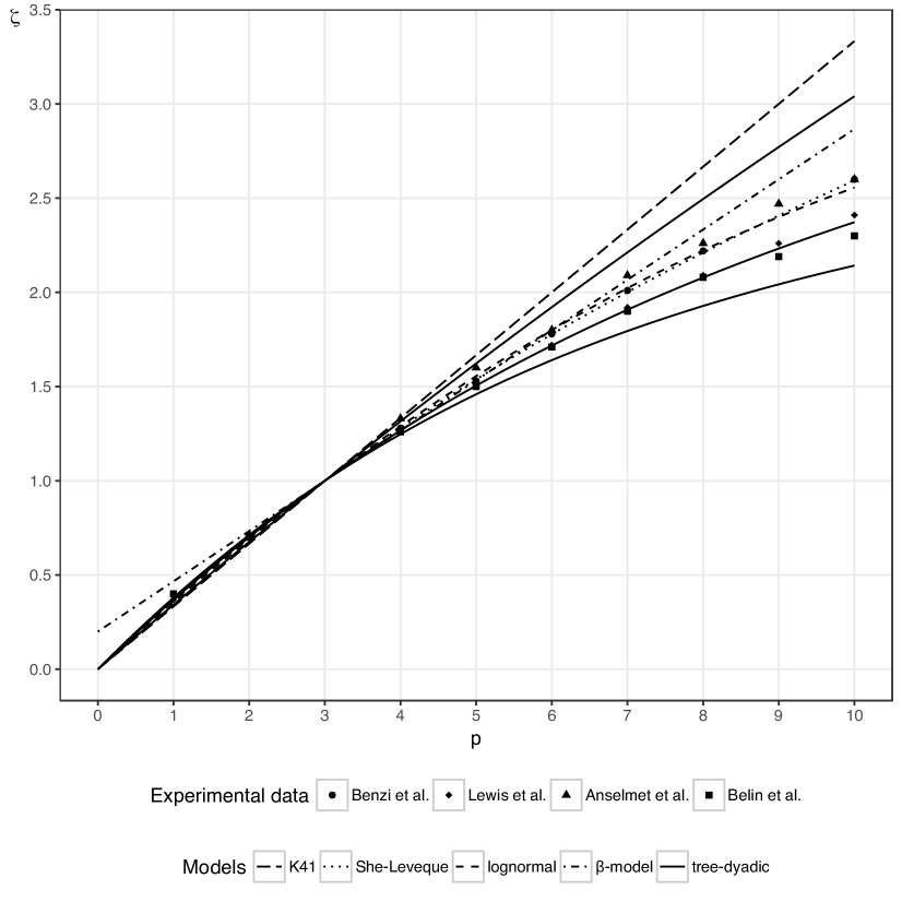
Figure 1: Comparison of $\zeta_{p}$ functions from different models and experimental data.

In Figure 1 we show the plots of the functions $\zeta_{p}$ for our model, with three different choices of parameters, and some of the other ones cited here, as well as experimental data from Anselmet et al. [2], Belin et al. [11], Benzi et al. [12] and Lewis et al. [40]. The choice of parameters is the following: in the log-normal model $\mu=0.2$, in the $\beta$ model $D=2.8$, in the tree-dyadic model

$$(\log_{2}\delta_{\omega})_{\omega}=(\lambda i,i=0,1,\dots,7)$$

with $\lambda=0.1$ for the top one, $\lambda=0.2$ for the middle one and $\lambda=0.2307$ for the bottom one.

Let us spend a couple more words on the choice of the coefficients for the RCM. Given the number of degrees of freedom we have in the choice of these coefficients (which are 7, since multiplicative constants for $\delta_{\omega}$ do not count), it is not particularly informative to show that we can fit precisely the experimental data. It is rather more interesting to show that, even considering just linear steps in the logarithms —to reduce to a family with one degree of freedom— we can cover quite a variety of situations. The extremal cases are upwards the Kolmogorov line K41, (corresponding to the flat model, with $\lambda=0$), and downwards $\lambda\approx 0.2307$ which is close to the constraint $h>0$.

5 Fractality

In this section we consider again the physical field $u(x)\coloneqq\sum_{j}u_{j}\psi_{j}(x)$ reconstructed from the constant solution of the RCM. It is defined on the physical space $Q_{\emptyset}$ and is multifractal in nature. In particular for every level of regularity (think of $C^{s}$ for example) there is a set of points $x$ for which $u$ around $x$ attains that regularity locally.

Anomalous dissipation depends on regularity; in the tradeoff between low regularity and high Hausdorff dimension of the set, we look for the critical set which accounts for most anomalous dissipation.

The first proposition computes the energy flow for a finite rooted subtree and explicits the term which we will identify with anomalous dissipation.

Proposition 5.1.

Let $T$ be a finite subset of $J$ with the property that $j\in T\Rightarrow\bar{\jmath}\in T$, Let $\partial T$ be the set of nodes outside $T$ with father in $T$ and let $v$ be a componentwise solution of (3). Then

$$\frac{d}{dt}\sum_{j\in T}v_{j}^{2}(t)=2f^{2}v_{\emptyset}(t)-\sum_{j\in\partial T}2c_{j}v_{\bar{\jmath}}(t)^{2}v_{j}(t).$$

Proof.

Since $T$ is finite we can exchange derivative and sum,

$$\frac{d}{dt}\sum_{j\in T}v_{j}^{2} =\sum_{j\in T}2v_{j}v_{j}^{\prime}=\sum_{j\in T}2v_{j}\biggl{(}c_{j}v_{\bar{\jmath}}^{2}-\sum_{k\in O(j)}c_{k}v_{j}v_{k}\biggr{)}$$

$$=\sum_{j\in T}2c_{j}v_{\bar{\jmath}}^{2}v_{j}-\sum_{k:\bar{k}\in T}2c_{k}v_{j}^{2}v_{k}.$$

By the hypothesis on $T$ and the definition of $\partial T$, we have

$$\{k\in J:\bar{k}\in T\}\cup\{\emptyset\}=T\cup\partial T.$$

Since the contribution of $\emptyset$ is $2f^{2}v_{\emptyset}(t)$, the proof is complete. ∎

Remark 9.

The generality of the set $T$ in Proposition 5.1 allows us to give an interpretation of the term $2c_{j}u_{\bar{\jmath}}^{2}u_{j}$ as the energy flow from $\bar{\jmath}$ to $j$. During each unit of time this amount of energy enters the subtree rooted in $j$ and distributes among all the subtree’s nodes, contributing to the wavelet components of the solution corresponding to these nodes. Notice that these components are all supported inside the cube $Q_{j}$, and we are considering the constant solution, so the same amount of energy must be dissipated inside the cube $Q_{j}$. Thus the quantity

$$F_{j}\coloneqq\frac{2c_{j}u_{\bar{\jmath}}^{2}u_{j}}{2c_{\emptyset}u_{\bar{\emptyset}}^{2}u_{\emptyset}}=\frac{1}{2^{q}f^{3}}c_{j}u_{\bar{\jmath}}^{2}u_{j},\qquad j\in J,$$ (17)

can be interpreted as the fraction of anomalous dissipation inside cube $Q_{j}$.

Notice moreover that if $T$ is as in Proposition 5.1, then the family $(Q_{j})_{j\in\partial T}$ forms a partition of $Q_{\emptyset}$ made of smaller non-overlapping cubes. In this sense Proposition 5.1 states that for any such partition of $Q_{\emptyset}$, the total energy dissipation of the system is the sum of the anomalous dissipation of every cube of the partition, and that this sum does not depend on the partition itself and it is always equal to the energy entering the system from its root.

The question arises now whether the anomalous dissipation is distributed somewhat evenly among the cubes of a partition. If this was the case, it would be more or less proportional to the volume of the cubes and there would be a density of anomalous dissipation with respect to the Lebesgue measure $\mathcal{L}$. This is not the case, as the following statement clarifies.

Proposition 5.2.

Let $u$ be the constant solution of an RCM, and $(F_{j})_{j\in J}$ defined as in (17). Let

$$\mathcal{R}(a)\coloneqq d+\frac{3}{2}\ell_{3/2}-\frac{3}{2}a,\qquad a\in\mathbb{R}.$$ (18)

Then the following holds:

1. Anomalous dissipation of energy in the cubes has an exponential rate in $|j|$ that can be computed explicitly:

   $$\frac{1}{|j|}\log_{2}F_{j}=-\mathcal{R}(\sigma_{j}),\qquad j\in J,$$ (19)

   where we define

   $$\sigma_{j}\coloneqq\frac{1}{|j|}\sum_{k\leq j}\log_{2}d_{k},\qquad j\in J.$$

2. Introduce the pointwise rate of anomalous dissipation,

   $$\sigma(x)\coloneqq\lim_{n\to\infty}\sigma_{x_{n}},$$

   for all $x\in Q_{\emptyset}$ for which the limit exists. Then $\sigma(x)=\ell_{0}$ for $\mathcal{L}$-a.e. $x$.

3. For all $x$ such that $\sigma(x)<\ell_{3/2}$,

   $$\lim_{n\to\infty}\frac{F_{x_{n}}}{\mathcal{L}(Q_{x_{n}})}=0.$$

   In particular if the model is not flat, then this holds for $\mathcal{L}$-a.e. $x$.

Proof.

By substituting the definition (14) inside (17), we get

$$F_{j}=2^{\alpha|j|}2^{3q|j|}\prod_{k\leq j}d_{k}^{3/2}.$$

We can now recall that, by (15), $q=-\frac{1}{3}\alpha-\frac{1}{3}d-\frac{1}{2}\ell_{3/2}$, so that

$$\frac{1}{|j|}\log_{2}F_{j}=\alpha+3q+\frac{3}{2}\frac{1}{|j|}\sum_{k\leq j}\log_{2}d_{k}=-d-\frac{3}{2}\ell_{3/2}+\frac{3}{2}\sigma_{j}=-\mathcal{R}(\sigma_{j}).$$

For the second part, consider the probability space $(Q_{\emptyset},\mathcal{B},\mathcal{L})$. The maps $x\mapsto d_{x_{i}}$, for $i\in{\mathbb{N}}$ are random variables, and so is $\sigma_{x_{n}}$,

$$\sigma_{x_{n}}=\frac{1}{n}\sum_{i=0}^{n}\log_{2}d_{x_{i}}.$$

By the definition of RCM, for all $i\in{\mathbb{N}}$ the law of $d_{x_{i}}$ conditioned on $d_{x_{i-1}}$ is uniform on the set $\{\delta_{\omega}\}_{\omega\in\Omega}$, hence the random process $(d_{x_{i}})_{i\in{\mathbb{N}}}$ is a sequence of i.i.d. random variables. By the strong law of large numbers,

$$\sigma_{x_{n}}\to\frac{1}{N}\sum_{\omega}\log_{2}\delta_{\omega}\qquad\mathcal{L}\text{-a.e. }x,\quad\text{as }n\to\infty.$$

By the definition of $\ell_{0}$ this completes the second part. As for the last part,

$$\frac{1}{n}\log_{2}\frac{F_{x_{n}}}{\mathcal{L}(Q_{x_{n}})}=\frac{1}{n}\log_{2}F_{x_{n}}+d,$$

and the right-hand side converges almost surely to $-\frac{3}{2}(\ell_{3/2}-\sigma(x))$ as $n\to\infty$.

The hypothesis that the model is not flat ensures that $\ell_{3/2}>\ell_{0}$. ∎

Proposition 5.2 states, in the first point, that the anomalous dissipation of cube $Q_{j}$ depends on $\sigma_{j}$. In particular if the anomalous dissipation was evenly distributed, $F_{j}$ would be proportional to the volume $2^{-dn}$ and hence by (19) the typical value of $\sigma_{j}$ would be $\ell_{3/2}$. On the contrary, the second point in Proposition 5.2 states that the typical value is $\ell_{0}$ instead, which is lesser, and cannot account for a positive fraction of the total anomalous dissipation (hence the 0 density limit). This means that anomalous dissipation is actually concentrated in few cubes with much larger values of $\sigma_{j}$ and $F_{j}$. This in turn suggests that we are dealing with a fractal object, and in particular that Lebesgue measure is not the right mathematical tool to get a meaningful picture of this phenomenon.

Remark 10.

From a local point of view, Proposition 5.2 further clarifies that pointwise anomalous dissipation happens exactly at the points $x$ such that $\sigma(x)\geq\ell_{3/2}$. This can be linked to some sort of local Hölder exponent, in fact the description of the spaces $C^{s}$ in terms of wavelet coefficients given in Definition 1 suggests a pointwise refinement by introducing the local Hölder exponent of $u$ at the point $x$ as

$$s(x):=\sup\left\{s:\sup_{n\geq 1}\biggl{(}ns+\frac{1}{2}dn+\log_{2}|u_{x_{n}}|\biggr{)}<\infty\right\},$$

or equivalently

$$s(x)=\liminf_{n\to\infty}\left(-\frac{d}{2}-\frac{1}{n}\log_{2}|u_{x_{n}}|\right).$$

Actually, there exists a different commonly accepted definition of local Hölder exponent: our $s(x)$ is in principle a different quantity (also found in the literature, often called the local singularity exponent of wavelet coefficients and denoted by $w(x)$). In many simple cases these two concepts are equivalent, but not in general, as is shown in Muzy et al. [44]. (We refer the reader to Riedi [51] for more details.)

In the case of the constant solution of the RCM we get

$$s(x)=\frac{1}{3}\biggl{(}\alpha-\frac{d}{2}\biggr{)}+\frac{1}{2}(\ell_{3/2}-\sigma(x)).$$

Then for the physical case, when $\alpha=1+d/2$, we get that $\sigma(x)\geq\ell_{3/2}$ if and only if $s(x)\leq\frac{1}{3}$: there is anomalous dissipation at a point $x$ if and only if $s(x)\leq\frac{1}{3}$. Notice that the “only if” part of this pointwise statement also holds for incompressible Euler equations, as was first shown by Duchon and Robert [27].

The following theorem, which could be restated in terms of a large deviation principle for $\sigma_{j}$, identifies exactly the single value of $\sigma_{j}$ which contributes to almost all the anomalous dissipation.

It will be useful to introduce the following function:

$$\varphi(\gamma)\coloneqq\sum_{\omega}\frac{\delta_{\omega}^{\gamma}}{\sum_{v}\delta_{v}^{\gamma}}\log_{2}\delta_{\omega},\qquad\gamma\in\mathbb{R},$$ (20)

which we notice satisfies

$$\frac{d}{d\gamma}(\gamma\ell_{\gamma})=\varphi(\gamma),\qquad\gamma\in\mathbb{R}.$$ (21)

Theorem 5.3.

For all sets $B\subset\mathbb{R}$ for which $\varphi(3/2)$ is an internal point,

$$\lim_{n\to\infty}\sum_{|j|=n}F_{j}\mathbbm{1}_{\sigma_{j}\in B}=1.$$

Remark 11.

Let $S_{a}\coloneqq\{x:\sigma(x)=a\}$. In non-rigorous terms, Theorem 5.3 states that the set $S_{\varphi(3/2)}$ accounts for all anomalous dissipation. Notice that $\varphi(3/2)\geq\ell_{3/2}$, as can be deduced by equation (22) below, so considering $S_{a}$ for increasing values of $a$, we get the picture that anomalous dissipation starts when $a=\ell_{3/2}$ and increases in intensity with $a$. When $a=\varphi(3/2)$ the tradeoff between intensity of anomalous dissipation and Hausdorff dimension of the set $S_{a}$ balances out and we may say that all anomalous dissipation happens in $S_{\varphi(3/2)}$.

To prove Theorem 5.3 we will need a couple of technical results.

Lemma 5.4.

Let $S$ be the canonical simplex of $\mathbb{R}^{\Omega}$,

$$S\coloneqq\{p\in\mathbb{R}_{+}^{\Omega}:\sum_{\omega\in\Omega}p_{\omega}=1\}.$$

Let $H$ be the entropy and $\sigma$ a linear function on $S$,

$$H(p)\coloneqq-\sum_{\omega\in\Omega}p_{\omega}\log_{2}p_{\omega},\qquad\qquad\sigma(p)\coloneqq\sum_{\omega\in\Omega}p_{\omega}\log_{2}\delta_{\omega}.$$

Suppose $\ell_{-\infty}\neq\ell_{\infty}$, then the map $\varphi$ defined by equation (20) is a strictly increasing bijection from $\mathbb{R}$ to $(\ell_{-\infty},\ell_{\infty})$. For all $a\in(\ell_{-\infty},\ell_{\infty})$ let $\gamma_{a}\coloneqq\varphi^{-1}(a)$. Then the maximum value of $H$ on $S$ subject to the constraint $\sigma(p)=a$ is

$$\mathcal{D}(a)\coloneqq d-\gamma_{a}(a-\ell_{\gamma_{a}})=\max_{\begin{subarray}{c}p\in S\\ \sigma(p)=a\end{subarray}}H(p)\leq d.$$ (22)

Otherwise, if $\ell_{-\infty}=\ell_{\infty}=:l$, then $\sigma(p)\equiv l$ is constant and

$$\max_{\begin{subarray}{c}p\in S\\ \sigma(p)=l\end{subarray}}H(p)=\max_{p\in S}H(p)=d\eqqcolon\mathcal{D}(l).$$

Remark 12.

Notice that $\mathcal{D}$ is defined differently in the two cases, but the two definitions are at least compatible, in the sense that in both cases $\mathcal{D}(\ell_{0})=d$.

Figure 2: Comparison of the functions $\ell$ and $\varphi$ for a given choice of coefficients $(\delta_{\omega})_{\omega\in\Omega}$.

Proof of Lemma 5.4.

If $\ell_{-\infty}=\ell_{\infty}$, then the model is flat, the $\delta_{\omega}$’s are all equal to $\delta=2^{l}$ and the constraint $\sigma(p)=l$ becomes trivially true. In that case $\mathcal{D}(a)$ is defined only for $a=l$ and equal to $d$, which is exactly the maximum of entropy under the single constraint of satisfying the simplex equation.

From now on we will suppose that the model is not flat. By the method of Lagrange multipliers applied to $H$ with two constraints given by $\sigma(p)=a$ and the simplex equation, we can immediately get that for any stationary point $\widehat{p}$,

$$\widehat{p}_{\omega}=c\delta_{\omega}^{\gamma},$$

for suitable constants $c$ and $\gamma$. From the simplex condition we have $c^{-1}=\sum_{\omega}\delta_{\omega}^{\gamma}$. From the other constraint we obtain

$$a=\sigma(\widehat{p})=\sum_{\omega\in\Omega}\widehat{p}_{\omega}\log_{2}\delta_{\omega}=\sum_{\omega\in\Omega}\frac{\delta_{\omega}^{\gamma}}{\sum_{v}\delta_{v}^{\gamma}}\log_{2}\delta_{\omega}=\varphi(\gamma).$$

The derivative of $\varphi$ is non-negative, since it can be expressed as the variance of a discrete random variable:

$$\varphi^{\prime}(\gamma)=\sum_{\omega}\frac{\delta_{\omega}^{\gamma}}{\sum_{v}\delta_{v}^{\gamma}}(\log_{2}\delta_{\omega})^{2}-\biggl{(}\sum_{\omega}\frac{\delta_{\omega}^{\gamma}}{\sum_{v}\delta_{v}^{\gamma}}\log_{2}\delta_{\omega}\biggr{)}^{2}\geq 0.$$

In particular $\varphi^{\prime}(\gamma)\neq 0$ since $\delta_{\omega}$ are not all equal and hence $\varphi$ is a bijection from $\mathbb{R}$ to $(\ell_{-\infty},\ell_{\infty})$.

We can thus invert $a=\varphi(\gamma)$, find $\gamma=\gamma_{a}=\varphi^{-1}(a)$ and compute $H(\hat{p})$

$$\begin{split}H(\widehat{p})&=-\sum_{\omega\in\Omega}\frac{\delta_{\omega}^{\gamma}}{\sum_{v}\delta_{v}^{\gamma}}\log_{2}\frac{\delta_{\omega}^{\gamma}}{\sum_{v}\delta_{v}^{\gamma}}\\ &=\log_{2}\sum_{v}\delta_{v}^{\gamma}-\sum_{\omega\in\Omega}\frac{\delta_{\omega}^{\gamma}}{\sum_{v}\delta_{v}^{\gamma}}\log_{2}\delta_{\omega}^{\gamma}=d+\gamma\ell_{\gamma}-\gamma\varphi(\gamma)=\mathcal{D}(a).\end{split}$$

To conclude it is enough to notice that $H$ is concave, since its Hessian matrix is diagonal negative definite. ∎

Lemma 5.5.

Consider the functions $\mathcal{R}$ and $\mathcal{D}$ as defined in equations (18) and (22). The following inequality holds:

$$\mathcal{R}(a)\geq\mathcal{D}(a),\qquad a\in(\ell_{-\infty},\ell_{\infty}),$$

with equality if and only if $a=\varphi(3/2)$.

Proof.

Let us consider the difference $\mathcal{R}(\varphi(\gamma))-\mathcal{D}(\varphi(\gamma))$ as a function of $\gamma$. We want to prove that

$$\frac{3}{2}\bigl{(}\ell_{3/2}-\varphi(\gamma)\bigr{)}-\gamma\bigl{(}\ell_{\gamma}-\varphi(\gamma)\bigr{)}\geq 0,$$

with equality if and only if $\gamma=\frac{3}{2}$. The if part of the equality case is obvious, while the strict inequality for $\gamma\neq\frac{3}{2}$ comes by Taylor formula for the function $s\mapsto s\ell_{s}$ in $\gamma$.

As we noticed in (21), we have for all $s$,

$$\frac{d}{ds}(s\ell_{s})=\varphi(s),$$

so we can write, for a suitable $\xi=\xi(s)\in(\gamma,s)$,

$$s\ell_{s}=\gamma\ell_{\gamma}+(s-\gamma)\varphi(\gamma)+\frac{1}{2}(s-\gamma)^{2}\varphi^{\prime}(\xi).$$

We proved in Lemma 5.4 that $\varphi$ is strictly increasing, so we get

$$s(\ell_{s}-\varphi(\gamma))-\gamma(\ell_{\gamma}-\varphi(\gamma))>0,$$

for all $s\neq\gamma$. ∎

We can now proceed with the proof of the theorem.

Proof of Theorem 5.3.

Let $n\geq 1$. Since $\sum_{|j|=n}F_{j}=1$ by the definition of $F_{j}$, the following defines a discrete probability measure on ${\mathbb{R}}$:

$$\mu_{n}\coloneqq\sum_{|j|=n}F_{j}\delta_{\sigma_{j}}.$$

Let $A$ be the complement of $B$ in ${\mathbb{R}}$. Having the result of Lemma 5.5 in mind, we will show that

$$\limsup_{n\to\infty}\frac{1}{n}\log_{2}\mu_{n}(A)\leq-\inf_{a\in A}\bigl{[}\mathcal{R}(a)-\mathcal{D}(a)\bigr{]}.$$ (23)

Assuming this to hold, by Lemma 5.5 and the hypothesis on $B$, namely that $\varphi(3/2)$ is an internal point, we will get

$$\inf_{a\in A}\bigl{[}\mathcal{R}(a)-\mathcal{D}(a)\bigr{]}\eqqcolon\lambda>0,$$

and hence

$$\mu_{n}(B)=1-\mu_{n}(A)\geq 1-2^{-\lambda^{\prime}n},$$

for $n$ large and a suitable $\lambda^{\prime}>0$, yielding the desired conclusion that $\mu_{n}(B)\to 1$ as $n\to\infty$.

To prove (23), we use Proposition 5.2 to rewrite $\mu_{n}(A)$ in terms of the $\sigma_{j}$’s as

$$\mu_{n}(A)\coloneqq\sum_{|j|=n}2^{n\bigl{(}-d-\frac{3}{2}\ell_{3/2}+\frac{3}{2}\sigma_{j}\bigr{)}}\delta_{\sigma_{j}}(A).$$

Notice that $\sigma_{j}=\sigma_{j^{\prime}}$ if $j$ and $j^{\prime}$ have the same generation and the $d_{k}$’s appear the same number of times but in different order in the definition of $\sigma_{j}$. This suggests the change of variables $p=\pi(j)$, where $\pi:J\to\mathbb{R}^{\Omega}$ is defined by

$$\pi_{\omega}(j)\coloneqq\frac{1}{|j|}\sharp\{k\leq j:d_{k}=\delta_{\omega}\},\qquad\omega\in\Omega,\quad j\in J.$$

In fact $\sigma_{j}$ depends only on $\pi(j)$, and indeed we can write $\sigma_{j}=\sigma(\pi(j))$, with $\sigma:\mathbb{R}^{\Omega}\to\mathbb{R}$ defined by

$$\sigma(p)\coloneqq\sum_{\omega\in\Omega}p_{\omega}\log_{2}\delta_{\omega},\qquad p\in\mathbb{R}^{\Omega}.$$

Now we can rewrite $\mu_{n}(A)$, with the change of variable $p=\pi(j)$, as

$$\mu_{n}(A)=\sum_{p\in S_{n}}\mathbbm{1}_{\sigma(p)\in A}2^{n(-d-\frac{3}{2}\ell_{3/2}+\frac{3}{2}\sigma(p))}c_{n}(p),$$

where

$$c_{n}(p)=\sharp\{j\in J:|j|=n,\pi(j)=p\},$$

and $S_{n}$ is the $\frac{1}{n}$-lattice inside the canonical symplex of $\mathbb{R}^{\Omega}$

$$\begin{split}S_{n}&=\pi(\{j\in J:|j|=n\})\\ &=\{p\in\mathbb{R}^{\Omega}:\sum_{v\in\Omega}p_{v}=1,\textup{ and for all }\omega\in\Omega,p_{w}\geq 0,p_{w}n\in{\mathbb{Z}}\}.\end{split}$$

We want an upper bound for $\mu_{n}(A)$. The factor $c_{n}(p)$ can be computed exactly, as it is easy to see that

$$c_{n}(p)=\binom{n}{p_{1}n\ p_{2}n\ \dots\ p_{N}n},$$

and this multinomial can be bounded by one version of Stirling’s approximation, yielding

$$\frac{1}{n}\log_{2}c_{n}(p)\leq\frac{1}{n}\log_{2}\left(\frac{n^{(1-N)/2}e}{(2\pi)^{N/2}}\prod_{\omega}p_{\omega}^{-p_{\omega}n+1/2}\right)\leq H(p)+C\frac{\log_{2}n}{n},$$

where $H$ denotes the entropy, defined as

$$H(p)=-\sum_{\omega}p_{\omega}\log_{2}p_{\omega},$$

and the constant $C$ does not depend on $p$ or $n$.

The sum over $S_{n}$ is then bounded by the cardinality $\sharp S_{n}$ times the supremum of the summand in $p$. We have

$$\sharp S_{n}=\binom{n+N-1}{N-1}\leq n^{N},$$

hence $\frac{1}{n}\log_{2}(\sharp S_{n})\leq N\frac{\log_{2}n}{n}$ and we get

$$\frac{1}{n}\log_{2}\mu_{n}(A)\leq(N+C)\frac{\log_{2}n}{n}+\sup_{p\in\sigma^{-1}(A)}\left(-d-\frac{3}{2}\ell_{3/2}+\frac{3}{2}\sigma(p)+H(p)\right).$$ (24)

By Lemma 5.4, $\sup_{p\in\sigma^{-1}(a)}H(p)=\mathcal{D}(a)$, so taking the limsup in(24), we get

$$\limsup_{n\to\infty}\frac{1}{n}\log_{2}\mu_{n}(A)\leq\sup_{a\in A}\left(-d-\frac{3}{2}\ell_{3/2}+\frac{3}{2}a+\mathcal{D}(a)\right),$$

which is a rewriting of (23). ∎

Finally, we deal with the Hausdorff dimension of the set of points that accounts for all anomalous dissipation. We will need to be more precise than we were in Remark 11. There we defined $S_{a}\coloneqq\{x:\exists\lim_{n}\sigma_{x_{n}}=a\}$. This will be now refined to $E(\mathbb{S}_{a})$, the set of $x$ for which all the points of accumulation of the relative densities of the $\delta_{\omega}$ appearing in the sequence $d_{x_{n}}$ correspond to $\sigma=a$. This notation allows us to use a theorem in Olsen [47] to compute the Hausdorff dimension of $E(\mathbb{S}_{a})$.

Consider once more the notation introduced in the proof of Theorem 5.3: the maps $\pi:J\to\mathbb{R}^{\Omega}$,

$$\pi_{\omega}(j)=\frac{1}{|j|}\sharp\{k\leq j:d_{k}=\delta_{\omega}\},\qquad\omega\in\Omega,\quad j\in J,$$

and $\sigma:\mathbb{R}^{\Omega}\to\mathbb{R}$,

$$\sigma(p)=\sum_{\omega\in\Omega}p_{\omega}\log_{2}\delta_{\omega},\qquad p\in\mathbb{R}^{\Omega}.$$

Consider moreover for $x\in Q_{\emptyset}$ the set of points of accumulation of the (vectorial) frequencies of the coefficients $(\delta_{\omega})_{\omega\in\Omega}$ in the dyadic expansion in $x$:

$$A(x)\coloneqq\operatorname{Acc}\Bigl{[}(\pi(x_{n}))_{n\geq 0}\Bigr{]}\subseteq S.$$

Let us also define

$$\mathbb{S}_{a}\coloneqq\{p\in S,\sigma(p)=a\},$$

and finally

$$E(\mathbb{S}_{a})\coloneqq\{x\in Q_{\emptyset}:A(x)\subseteq\mathbb{S}_{a}\},$$

the set of all points $x$ in the cube $Q_{\emptyset}$ such that the asymptotic frequencies of the $(\delta_{\omega})_{\omega\in\Omega}$ associated to $x$ are in $\mathbb{S}_{a}$.

With the notation introduced above, the following theorem was proved by Olsen (see [47])

Theorem 5.6 (Olsen).

The Hausdorff dimension of $E(\mathbb{S}_{a})$ is:

$$\dim E(\mathbb{S}_{a})=\sup_{p\in\mathbb{S}_{a}}H(p).$$

Thanks to Lemma 5.4, we can compute this dimension for all $a$, and in particular, by Theorem 5.3 we obtain the following statement.

Theorem 5.7.

For all $a\in[\ell_{-\infty},\ell_{+\infty}]$, the Hausdorff dimension of the set $E(\mathbb{S}_{a})$ is $\mathcal{D}(a)$. In particular the Hausdorff dimension of the set of the points $x$ where anomalous dissipation occurs is

$$\Delta=d-\frac{3}{2}\bigl{(}\varphi(3/2)-\ell_{3/2}\bigr{)}.$$

Remark 13.

It is worth noting that the value of $\Delta$ is in agreement with what was expected in the framework of the Frisch-Parisi multifractal model [49], that is

$$\Delta=3\zeta^{\prime}_{3}+d-1$$

Heuristically, the multifractal formalism relates the Hausdorff dimension $d(h)$ of the sets of points of given Hölder exponent $h$ with $\zeta_{p}$ through a Legendre transform:

$$\zeta_{p}=\min_{h}(ph-d(h))+d,\qquad d-d(h)=\max_{p}(\zeta_{p}-ph).$$

If a point $x$ has Hölder exponent $h(x)$, then it is expected that the measure of energy dissipation has in $x$ a singularity exponent $\nu(x)=3h(x)-1+d$ (this can be deduced by the formula for $F_{j}$, with $\alpha=1+d/2$). Let $\nu:=3h-1+d$, then

$$d-d(h)\geq\zeta_{3}-3h=d-\nu$$

for all $h$, with equality only for $h=\zeta_{3}^{\prime}$. Then summing up all energy dissipation at points $x$ with $h(x)=h$ we get

$$\mathcal{E}(h)\leq\limsup_{n}2^{d(h)n}2^{-\nu n},$$

hence the only contribution is for $h=\zeta^{\prime}_{3}$ and so $\Delta=d(\zeta^{\prime}_{3})$ as claimed.

Appendix A Appendix

In this section we propose an heuristic argument to justify formula (5) given in Section 2.2 for the exponent of the structure function.

Let $(\psi_{j})_{j\in J}$ be a family of wavelets such that $\psi_{j}$ is essentially supported on the cube $Q_{j}$ and they are all rescaled and translated versions one of the other:

$$\psi_{j}(x)=2^{d|j|/2}\psi_{\emptyset}(2^{|j|}x+\theta_{j}),$$

for some “mother wavelet” $\psi_{\emptyset}$. We consider real values $(u_{j})_{j\in J}$ and pose $u(x):=\sum_{j\in J}u_{j}\psi_{j}(x)$, for all $x\in Q_{\emptyset}$, and define as usual the structure function

$$S_{p}(r):=\int_{Q_{\emptyset}}\left\langle|u(x)-u(y)|^{p}\right\rangle_{y}dx,$$

where $\langle\cdot\rangle_{y}$ denotes the average on the points $y$ such that $|y-x|=r$, and its exponents,

$$\zeta_{p}:=-\lim_{n\to\infty}\frac{1}{n}\log_{2}S_{p}(2^{-n}).$$

We introduce also the function

$$\xi_{p}:=d-\frac{p}{2}d-\limsup_{n\to\infty}\frac{1}{n}\log_{2}\sum_{|j|=n}|u_{j}|^{p},\qquad p\geq 0.$$

We want to show that under suitable hypothesis, if $\xi_{p}>0$, then $\zeta_{p}=\min(p,\xi_{p})$.

Remark 14.

For any map $\varphi:J\to{\mathbb{R}}$, for almost every $x\in Q_{\emptyset}$,

$$\sum_{j\in J}\varphi(j)\psi_{j}(x)=\sum_{i\geq 0}\varphi(x_{i})\psi_{x_{i}}(x).$$

Lemma A.1.

Let $(a_{i})_{i\geq 0}$ be a sequence of positive numbers. Let $\lambda>1$ and $p\geq 1$, then

$$\biggl{(}\sum_{k\geq 0}a_{k}\biggr{)}^{p}\leq c(\lambda,p)\sum_{k\geq 0}\lambda^{k}a_{k}^{p},$$

where $c(\lambda,p)=1$ for $p=1$ and $c(\lambda,p)=\bigl{(}1-\lambda^{-1/(p-1)}\bigr{)}^{-(p-1)}$ otherwise.

Proof.

Simply apply Hölder inequality to $\sum_{k\geq 0}a_{k}=\int\lambda^{-k}a_{k}d\mu(k)$ where $\mu$ is the discrete measure on the non-negative integers defined by $\mu(k):=\lambda^{k}$. ∎

Lemma A.2.

If $\xi_{p}>0$, then $u\in L^{p}(Q_{\emptyset})$.

Proof.

By Remark 14 and Lemma A.1, for all $\lambda>1$,

$$\begin{split}\|u\|_{L^{p}}^{p}&\leq\int_{Q_{\emptyset}}\Bigl{(}\sum_{i\geq 0}|u_{x_{i}}\psi_{x_{i}}(x)|\Bigr{)}^{p}dx\leq c(\lambda,p)\int_{Q_{\emptyset}}\sum_{i\geq 0}\lambda^{i}|u_{x_{i}}\psi_{x_{i}}(x)|^{p}dx\\ &=c(\lambda,p)\int_{Q_{\emptyset}}\sum_{j\in J}\lambda^{|j|}|u_{j}\psi_{j}(x)|^{p}dx\leq c_{1}(\lambda,p)\sum_{j\in J}\lambda^{|j|}|u_{j}|^{p}2^{(dp/2-d)|j|}\\ &=c_{1}(\lambda,p)\sum_{i\geq 0}\lambda^{i}2^{-\xi_{p}i}.\qed\end{split}$$

We need to introduce an hypothesis on the function $u$, in that it needs to show some sort of autosimilarity with respect to the wavelet decomposition, as clarified below.

To do so, we need to introduce the sets of automorphisms on $J$, that is

$$S\coloneqq\{\sigma:J\to J\,|\,\sigma(\emptyset)=\emptyset,\sigma(k)=\sigma(\bar{\jmath})\text{ iff }k=\bar{\jmath}\}.$$

Autosimilarity hypothesis.

For all $j\in J$ there exists $\sigma_{j}\in S$ such that for all $k\in J$,

$$u_{jk}\sim u_{j}u_{\sigma_{j}(k)}.$$

Here with $\sim$ we intend that the absolute value of the ratio between the two terms is uniformly bounded from above and below, away from zero.

(Notice that the unique constant solution of an RCM trivially satisfies this hypothesis.)

Lemma A.3.

For all $n\geq 0$, under autosimilarity hypothesis,

$$\int_{Q_{\emptyset}}\Bigl{|}\sum_{|j|\geq n}u_{j}\psi_{j}(x)\Bigr{|}^{p}dx\sim\|u\|_{L^{p}}^{p}2^{(\frac{d}{2}p-d)n}\sum_{|j|=n}|u_{j}|^{p}.$$

Proof.

Any automorphism $\sigma\in S$ induces a measure-preserving map $\sigma$ on $Q_{\emptyset}$, defined by $Q_{\emptyset}\ni x=(x_{0},x_{1},x_{2},\dots)\mapsto\sigma(x):=(\sigma(x_{0}),\sigma(x_{1}),\dots)$, so that $\psi_{\sigma^{-1}(k)}(z)=\psi_{k}(\sigma(z))$.

Then, for any $j\in J$ with $|j|=n$, by the two hypothesis,

$$\begin{split}\sum_{k\geq j}u_{k}\psi_{k}(x)&=\sum_{k\in J}u_{jk}\psi_{jk}(x)\\ &\sim\sum_{k\in J}u_{j}u_{\sigma_{j}(k)}2^{\frac{d}{2}|j|}\psi_{k}(2^{|j|}x+\theta_{j})\sim 2^{\frac{d}{2}|j|}u_{j}u(\sigma_{j}(z)),\end{split}$$

where $z=z(x,j)=2^{|j|}x+\theta_{j}$ spans $Q_{\emptyset}$ as $x$ spans $Q_{j}$. Thus

$$\begin{split}\int_{Q_{\emptyset}}\Bigl{|}\sum_{|j|\geq n}u_{j}\psi_{j}(x)\Bigr{|}^{p}dx&\sim 2^{\frac{d}{2}np}\sum_{|j|=n}|u_{j}|^{p}\int_{Q_{j}}|u(\sigma_{j}(z))|^{p}dx\\ &\sim\|u\|_{L^{p}}^{p}2^{(\frac{d}{2}p-d)n}\sum_{|j|=n}|u_{j}|^{p}.\qed\end{split}$$

We decompose the difference appearing in $S_{p}$ as follows:

$$u(x)-u(y)=\sum_{|j|<n}u_{j}(\psi_{j}(x)-\psi_{j}(y))+\sum_{|j|\geq n}u_{j}\psi_{j}(x)-\sum_{|j|\geq n}u_{j}\psi_{j}(y).$$

For the first terms, when $|j|<n$,

$$|\psi_{j}(x)-\psi_{j}(y)|\approx|\nabla\psi_{j}||x-y|\mathbbm{1}_{Q_{j}}(x)\approx 2^{(\frac{d}{2}+1)|j|}2^{-n}\mathbbm{1}_{Q_{j}}(x),$$

and in particular

$$\int_{Q_{\emptyset}}\Bigl{\langle}\Bigl{|}\sum_{|j|=i}u_{j}(\psi_{j}(x)-\psi_{j}(y))\Bigr{|}^{p}\Bigr{\rangle}_{y}dx\approx 2^{[(\frac{d}{2}+1)p-d]i-np}\sum_{|j|=i}|u_{j}|^{p}.$$

Using Lemma A.3 to estimate the two remaining sums and putting everything together, we get that for $\xi_{p}>0$,

$$S_{p}(2^{-n})\approx n^{p}2^{-np}\sum_{i=0}^{n}2^{[(\frac{d}{2}+1)p-d]i}\sum_{|j|=i}|u_{j}|^{p}\approx 2^{-np}\sum_{i=0}^{n}2^{(p-\xi_{p})i}\approx 2^{-\min(p,\xi_{p})n}$$

hence we have the claimed result,

$$-\lim_{n\to\infty}\frac{1}{n}\log_{2}S_{p}(2^{-n})=:\zeta_{p}=\min(p,\xi_{p}).$$

References

- [1] L. Andreis, D. Barbato, F. Collet, M. Formentin, and L. Provenzano. Strong existence and uniqueness of the stationary distribution for a stochastic inviscid dyadic model. Nonlinearity, 29(3):1156, 2016.
- [2] F. Anselmet, Y. Gagne, E. Hopfinger, and R. Antonia. High-order velocity structure functions in turbulent shear flows. Journal of Fluid Mechanics, 140(1):63–89, 1984.
- [3] A. Arneodo, E. Bacry, and J. Muzy. Random cascades on wavelet dyadic trees. Journal of Mathematical Physics, 39(8):4142–4164, 1998.
- [4] D. Barbato, L. A. Bianchi, F. Flandoli, and F. Morandin. A dyadic model on a tree. Journal of Mathematical Physics, 54:021507, 2013.
- [5] D. Barbato, F. Flandoli, and F. Morandin. A theorem of uniqueness for an inviscid dyadic model. C. R. Math. Acad. Sci. Paris, 348(9-10):525–528, 2010.
- [6] D. Barbato, F. Flandoli, and F. Morandin. Anomalous dissipation in a stochastic inviscid dyadic model. Ann. Appl. Probab., 21(6):2424–2446, 2011.
- [7] D. Barbato and F. Morandin. Positive and non-positive solutions for an inviscid dyadic model: well-posedness and regularity. Nonlinear Differential Equations and Applications NoDEA, 20(3):1105–1123, 2013.
- [8] D. Barbato, F. Morandin, and M. Romito. Smooth solutions for the dyadic model. Nonlinearity, 24(11):3083, 2011.
- [9] D. Barbato, F. Morandin, and M. Romito. Global regularity for a slightly supercritical hyperdissipative Navier–Stokes system. Analysis & PDE, 7(8):2009–2027, 2015.
- [10] J. Barral, X. Jin, and B. t. Mandelbrot. Convergence of complex multiplicative cascades. Ann. Appl. Probab., 20(4):1219–1252, 2010.
- [11] F. Belin, P. Tabeling, and H. Willaime. Exponents of the structure functions in a low temperature helium experiment. Physica D: Nonlinear Phenomena, 93(1):52–63, 1996.
- [12] R. Benzi, L. Biferale, S. Ciliberto, M. Struglia, and R. Tripiccione. Generalized scaling in fully developed turbulence. Physica D: Nonlinear Phenomena, 96(1):162–181, 1996.
- [13] R. Benzi, L. Biferale, A. Crisanti, G. Paladin, M. Vergassola, and A. Vulpiani. A random process for the construction of multiaffine fields. Physica D: Nonlinear Phenomena, 65(4):352–358, 1993.
- [14] R. Benzi, L. Biferale, and G. Parisi. On intermittency in a cascade model for turbulence. Physica D: Nonlinear Phenomena, 65(1-2):163–171, 1993.
- [15] R. Benzi, L. Biferale, R. Tripiccione, and E. Trovatore. (1+ 1)-dimensional turbulence. Physics of Fluids, 9:2355, 1997.
- [16] R. Benzi, G. Paladin, G. Parisi, and A. Vulpiani. On the multifractal nature of fully developed turbulence and chaotic systems. Journal of Physics A: Mathematical and General, 17(18):3521, 1984.
- [17] L. A. Bianchi. Uniqueness for an inviscid stochastic dyadic model on a tree. Electronic Communications in Probability, 18:1–12, 2013.
- [18] L. Biferale. Shell models of energy cascade in turbulence. Annu. Rev. Fluid Mech., 35:441–468, 2003.
- [19] T. Buckmaster. Onsager’s conjecture almost everywhere in time. Communications in Mathematical Physics, 333(3):1175–1198, 2015.
- [20] T. Buckmaster, C. De Lellis, and L. Székelyhidi. Dissipative Euler flows with Onsager-critical spatial regularity. Communications on Pure and Applied Mathematics, 2015.
- [21] A. Cheskidov and S. Friedlander. The vanishing viscosity limit for a dyadic model. Phys. D, 238(8):783–787, 2009.
- [22] A. Cheskidov, S. Friedlander, and N. Pavlović. Inviscid dyadic model of turbulence: the fixed point and Onsager’s conjecture. J. Math. Phys., 48(6):065503, 16, 2007.
- [23] A. Cheskidov, S. Friedlander, and N. Pavlović. An inviscid dyadic model of turbulence: the global attractor. Discrete Contin. Dyn. Syst., 26(3):781–794, 2010.
- [24] P. Constantin, W. E, and E. S. Titi. Onsager’s conjecture on the energy conservation for solutions of Euler’s equation. Communications in Mathematical Physics, 165(1):207–209, 1994.
- [25] E. Deriaz and V. Perrier. Divergence-free and curl-free wavelets in two dimensions and three dimensions: application to turbulent flows. Journal of Turbulence, 7(3):1–37, 2006.
- [26] V. N. Desnianskii and E. A. Novikov. Simulation of cascade processes in turbulent flows. Prikladnaia Matematika i Mekhanika, 38:507–513, 1974.
- [27] J. Duchon and R. Robert. Inertial energy dissipation for weak solutions of incompressible Euler and Navier-Stokes equations. Nonlinearity, 13(1):249–255, 2000.
- [28] H. Eggleston. The fractional dimension of a set defined by decimal properties. The Quarterly Journal of Mathematics, 20:31–36, 1949.
- [29] G. L. Eyink. Energy dissipation without viscosity in ideal hydrodynamics i. fourier analysis and local energy transfer. Physica D: Nonlinear Phenomena, 78(3):222–240, 1994.
- [30] G. L. Eyink. Besov spaces and the multifractal hypothesis. Journal of Statistical Physics, 78(1-2):353–375, 1995.
- [31] S. Friedlander and N. Pavlović. Blowup in a three-dimensional vector model for the Euler equations. Comm. Pure Appl. Math., 57(6):705–725, 2004.
- [32] U. Frisch. Turbulence. Cambridge University Press, Cambridge, 1995. The legacy of A. N. Kolmogorov.
- [33] U. Frisch, P.-L. Sulem, and M. Nelkin. A simple dynamical model of intermittent fully developed turbulence. Journal of Fluid Mechanics, 87(04):719–736, 1978.
- [34] E. Gledzer. System of hydrodynamic type admitting two quadratic integrals of motion. In Soviet Physics Doklady, volume 18, page 216, 1973.
- [35] P. Isett. Hölder Continuous Euler Flows in Three Dimensions with Compact Support in Time, volume 196 of Annals of Mathematics Studies. Princeton University Press, Princeton, NJ, 2017.
- [36] S. Jaffard. Multifractal formalism for functions part i: results valid for all functions. SIAM Journal on Mathematical Analysis, 28(4):944–970, 1997.
- [37] N. H. Katz and N. Pavlović. Finite time blow-up for a dyadic model of the Euler equations equations. Trans. Amer. Math. Soc., 357(2):695–708 (electronic), 2005.
- [38] A. N. Kolmogorov. The local structure of turbulence in incompressible viscous fluids at very large Reynolds numbers. Dokl. Akad. Nauk. SSSR, 30:301–305, 1941.
- [39] A. N. Kolmogorov. A refinement of previous hypotheses concerning the local structure of turbulence in a viscous incompressible fluid at high Reynolds number. J. Fluid Mech., 13:82–85, 1962.
- [40] G. S. Lewis and H. L. Swinney. Velocity structure functions, scaling, and transitions in high-reynolds-number couette-taylor flow. Phys. Rev. E, 59:5457–5467, May 1999.
- [41] B. B. Mandelbrot. Intermittent turbulence in self-similar cascades: divergence of high moments and dimension of the carrier. Journal of fluid Mechanics, 62(2):331–358, 1974.
- [42] C. Meneveau and K. Sreenivasan. The multifractal nature of turbulent energy dissipation. Journal of Fluid Mechanics, 224:429–484, 1991.
- [43] Y. Meyer. Wavelets and operators, volume 37 of Cambridge Studies in Advanced Mathematics. Cambridge University Press, Cambridge, 1992. Translated from the 1990 French original by D. H. Salinger.
- [44] J.-F. Muzy, E. Bacry, and A. Arneodo. Multifractal formalism for fractal signals: The structure-function approach versus the wavelet-transform modulus-maxima method. Physical review E, 47(2):875, 1993.
- [45] A. Obukhov. Some specific features of atmospheric turbulence. Journal of Geophysical Research, 67(8):3011–3014, 1962.
- [46] K. Ohkitani and M. Yamada. Temporal intermittency in the energy cascade process and local lyapunov analysis in fully-developed model turbulence. Progress of theoretical physics, 81(2):329–341, 1989.
- [47] L. Olsen. On the Hausdorff dimension of generalized Besicovitch-Eggleston sets of -tuples of numbers. Indagationes Mathematicae, 15(4):535–547, 2004.
- [48] L. Onsager. Statistical hydrodynamics. Il Nuovo Cimento (1943-1954), 6:279–287, 1949.
- [49] G. Parisi and U. Frisch. On the singularity structure of fully developed turbulence. In Turbulence and Predictability in Geophysical Fluid Dynamics. Proc. Intl. School of Physics E. Fermi, pages 84–87. Amsterdam, The Netherlands, 1985.
- [50] V. Perrier and C. Basdevant. Besov norms in terms of the continuous wavelet transform. application to structure functions. Mathematical Models and Methods in Applied Sciences, 6(05):649–664, 1996.
- [51] R. H. Riedi. Multifractal processes. Technical report, DTIC Document, 1999.
- [52] Z.-S. She and E. Leveque. Universal scaling laws in fully developed turbulence. Physical review letters, 72(3):336, 1994.
- [53] R. Stevenson. Divergence-free wavelet bases on the hypercube. Applied and Computational Harmonic Analysis, 30(1):1–19, 2011.
- [54] T. Tao. Finite time blowup for an averaged three-dimensional Navier-Stokes equation. Journal of the American Mathematical Society, 2015.