Naturalness from a Composite Top?

Abstract

We consider a theory with composite top quarks but an elementary Higgs boson. The hierarchy problem can be solved by supplementing TeV scale top compositeness with either supersymmetry or Higgs compositeness appearing at the multi-TeV scale. The Higgs boson couples to uncolored partons within the top quark. We study how this approach can give rise to a novel screening effect that suppresses production of the colored top partners at the LHC. Strong constraints arise from $Z$ to $\bar{b}b$, as well potentially from flavor physics. Independent of flavor considerations, current constraints imply a compositeness scale $\!\mathrel{\hbox{\hbox to0.0pt{\lower 2.36806pt\hbox{$\sim$}\hss} \kern-3.39996pt\raise 1.72218pt\hbox{$>$}}}$ TeV; this implies that the model is likely tuned at the percent level. Four top quark production at the LHC is a smoking-gun probe of this scenario. New CP violation in D meson mixing is also possible.

I Introduction

The large top quark Yukawa coupling $y_{t}\approx 1$ produces the dominant corrections to the Standard Model (SM) Higgs boson (mass)²: $\Delta m_{h}^{2}\sim\frac{3y_{t}^{2}}{4\pi^{2}}\Lambda^{2}$. Here, $\Lambda$ is a UV cut-off scale at which new physics appears to cancel the quadratic divergence. If $\Lambda$ is much larger than the electroweak (EW) scale, these large quantum corrections combine with a nearly equal and opposite bare contribution to yield the much smaller weak scale Susskind (1979). This apparent conspiracy is known as the fine-tuning or gauge hierarchy problem.

In most solutions to the hierarchy problem, colored particles near the weak scale provide the necessary cutoff $\Lambda$. For example, in supersymmetry (SUSY) the superpartner of top quark does the job. In this paper, we instead assume that the third generation of quarks are composite particles that emerge after the confinement of a strongly coupled gauge group, which happens the TeV scale. Contrary to most theories of strong dynamics, we assume the Higgs boson is an elementary scalar and couples to some of the color neutral partonic constituents of the top quark. The top Yukawa coupling is an induced coupling from the low-energy effective theory point of view. This setup separates the Yukawa coupling (responsible for the Higgs mass correction), from the $SU(3)_{c}$ charge (potentially a source of stringent collider constraints).

Composite top quarks composite do not stabilize the Higgs (mass)² by themselves. Above the compositeness scale, a quadratic contribution to the elementary Higgs (mass)² remains, arising from Yukawa interactions with the color neutral partons. An additional mechanism – such as SUSY at a slightly higher energy scale – is needed to cancel this contribution. This additional mechanism likely introduces colored top partners after the strong dynamics confines, but we will show hadronization under the new strong dynamics suppresses the production of those heavy $SU(3)_{c}$ colored states.

In our model, the 1-loop quadratically divergent correction to Higgs mass can be split into two pieces:

$$\delta m_{H}^{2}\simeq\frac{3y_{t}^{2}}{4\pi^{2}}\Lambda_{C}^{2}+\frac{Ny_{\psi}^{2}}{4\pi^{2}}\Lambda_{\psi}^{2}.$$ (1)

Here, $\Lambda_{C}$ is the confinement scale of our new strong gauge interaction, and $\Lambda_{\psi}$ is the UV scale where additional (presumably colorless) new physics should be introduced to cancel the corrections from the colorless partons $\psi$ to the Higgs mass. The basic idea is summarized in Fig. 1. We will find consistency with current bounds from precision electroweak constraints and collider searches requires $\Lambda_{C}\!\mathrel{\hbox{\hbox to0.0pt{\lower 2.36806pt\hbox{$\sim$}\hss} \kern-3.39996pt\raise 1.72218pt\hbox{$>$}}}$ TeV. The strongly coupled nature of the theory introduces uncertainty in this estimate.

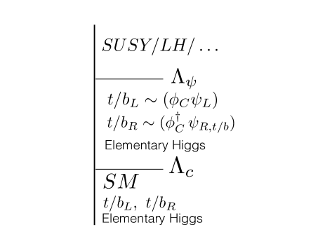
Figure 1: Above $\Lambda_{C}$ the top/bottom quark is revealed to be composites. Above $\Lambda_{\psi}$ additional physics enters (e.g. supersymmetry or a Little Higgs model) to eliminate remaining quadratic divergences to the Higgs boson mass.

The idea of composite top quarks has a long history Georgi et al. (1995), with recent discussions in Pomarol and Serra (2008), and emphasis on collider signals in Lillie et al. (2008); Kumar et al. (2009); Fabbrichesi et al. (2014); Englert et al. (2014). There are also a host of theories where the Higgs boson is composite, and the top is largely composite Kaplan (1991), for reviews, see Contino et al. (2007); Panico and Wulzer (2016). In our set-up, however, we imagine that the Higgs boson is still an elementary scalar. This impacts the pattern of low-energy deviations from the Standard Model as well as the way in which the model should be UV completed above the compositeness scale.

In the following section, we discuss the relationship between the partonic Yukawa coupling and the induced effective Yukawa coupling between the Higgs and the top quark. We will see the partonic Yukawa coupling might even be ${\mathcal{O}}(0.1)$ while remaining consistent with an ${\mathcal{O}(1)}$ top Yukawa coupling. We then discuss an important constraint on the confining theory: confinement must occur without chiral symmetry breaking. If this were not the case, the top quark would get a too large mass. In Sec. IV, we discuss UV models which may be present above the confinement scale $\Lambda_{C}$ to truncate the remaining quadratic divergences from the Yukawa couplings between the Higgs and color neutral partons. In Sec. V, we note how the hadronization of the new strong interaction can dramatically reduce the production of heavy $SU(3)_{c}$ colored composite states with mass above $\Lambda_{C}$. Although the existence of these states are unavoidable, this screening effect removes or delays the appearance of these particles at a hadron collider. Then, in Sec. VI, we review phenomenological bounds on our scenario, both from low-energy probes and from direct probes of compositeness at the LHC. Some additional flavor constraints appear in an Appendix. In Sec. VII, we discuss the collider signatures of this model as energies approach the compositeness scale. In another appendix, we make some comments regarding anomaly cancelation and how this module might be embedded in a UV theory.

II Induced top Yukawa

The Yukawa coupling between the top quark and Higgs boson is induced by the Yukawa coupling between colorless partons $\psi_{L/R}^{\alpha}$ within the top and the Higgs boson, i.e. $y_{\psi}H\psi_{L}\psi_{R}$. The form factors translating the partonic coupling $y_{\psi}$ to the bound state coupling $y_{t}$ are not known. One might worry whether the partonic Yukawa coupling needs to be very large to achieve a ${\mathcal{O}}(1)$ top Yukawa coupling. If that were the case, it would not be attractive from a naturalness point of view: the quadratic divergence from the partons would become larger than that from top quark, see Eq. (1). The relationship between the Yukawa couplings can be estimated by naïve dimensional analysis (NDA) Manohar and Georgi (1984); Georgi and Randall (1986), see also Jenkins et al. (2013). The effective Lagrangian can be written as

$$\mathscr{L}_{NDA}\supset f^{2}\Lambda_{C}^{2}\bigg{(}\frac{y_{\psi}H}{\Lambda_{C}}\bigg{)}\bigg{(}\frac{Q}{f\sqrt{\Lambda_{C}}}\bigg{)}\bigg{(}\frac{t_{R}}{f\sqrt{\Lambda_{C}}}\bigg{)}=y_{\psi}HQt_{R}.$$ (2)

Here, $\Lambda_{C}$ represents the scale of compositeness – the confinement scale of the new strong dynamics. We take the dimensionful parameter associated with Higgs as $\Lambda_{C}$ instead of $f$ (as is done in composite Higgs scenarios). This is because the Higgs is an elementary particle that does not participate in the strong dynamics. $\Lambda_{C}\equiv g_{\ast}f$, where $g_{\ast}$ is a typical strong coupling. In NDA, it is taken to be $g_{\ast}\simeq 4\pi$. (We define $g_{\ast}$ as having no N-dependence; we will discuss the subtlety of N-dependence later.) So, NDA predicts $y_{t}\simeq y_{\psi}$. Although NDA only provides guidance on the magnitude of couplings in the low-energy effective theory, it at least indicates the Yukawa coupling between the Higgs and top quarks is not dramatically suppressed.

We can potentially gain further insight into the translation between the parton-level and low-energy effective theory Yukawa couplings by studying a similar scenario in the SM. There, we can discuss how the coupling of the Higgs boson to the proton relates to the underlying couplings between the Higgs and the quarks. These form factors are well-studied, e.g. in the context of dark matter direct detection, and we quote the results Cheng (1989); Belanger et al. (2014):

$$B^{n,p}_{u,d} \equiv \frac{y_{u,d}}{y^{n,p}_{u,d}}\sim{\mathcal{O}}(0.1),$$ (3)

$$B^{n,p}_{s} \equiv \frac{y_{s}}{y^{n,p}_{s}}\sim{\mathcal{O}}(1).$$ (4)

We have defined $y^{n,p}_{q}$ in terms of the usual nucleon parameters as: $y^{n,p}_{q}\equiv m_{N}f^{T}_{q}/v$, where $v$ is the electroweak vacuum expectation value (VEV) and $m_{N}$ the nucleon mass. We emphasize these equations describe the relationship between the quark Yukawa couplings and the induced Higgs-nucleon-nucleon coupling. The results of Eqs. (3),(4) are roughly consistent with NDA expectations.

It is not unreasonable that the form factors may in fact deviate from one. Scalar field interactions with sea-quarks add; there is no cancellation between particle and anti-particle. So, it may be that $y_{\psi}$ smaller than $y_{t}$, say $y_{\psi}\sim 0.1$. This would effectively postpone the need for new states which cut off divergences from the Higgs coupling to $\psi_{L/R}$.

III Confinement without chiral condensation

The partons comprising the top quarks are assumed to be fermionic and massless. Their masses are protected by chiral symmetry. However, this is insufficient to ensure top quarks remain massless after confinement. Indeed, after QCD confines, the only light hadrons with $m<<\Lambda_{QCD}$ are pions and kaons, which are pseudo-Nambu-Goldstone bosons from the spontaneously broken approximate chiral symmetry. There are no light fermions after QCD confines. This is because chiral condensation occurs at a similar scale to QCD confinement, $\langle\bar{q}q\rangle\sim 4\pi f_{\pi}^{3}$. If our strong dynamics were to simultaneously confine and break chiral symmetry, we would expect the top quark would get mass at the confinement scale, just like the proton of QCD. This would mean a too large top mass of ${\mathcal{O}}$(TeV).

But chiral symmetry breaking need not happen when the gauge group confines. SUSY QCD provides an existence proof: for an $SU(N_{c})$ gauge group with $N_{F}=N_{C}+1$, there are massless fermions at the origin of the moduli space of the dual theory. Those massless fermions are bound states of the elementary particles in the theory before duality Seiberg (1994). Confinement without chiral condensation has also been studied in early attempts to explore the SM as a relic a strongly coupled theory, see, e.g. Raby et al. (1980); Dimopoulos et al. (1980).

While we are agnostic as to the identity of the new strong gauge group, for concreteness we refer to it as $SU(N)$. We assume $SU(N)$ confinement occurs without chiral condensation, and the top quark mass comes from the VEV of the Higgs alone. The massless composite fermions are written as bound states of a scalar boson $\phi_{c}$ and a fermion $\psi_{L/R}^{\alpha}$. As mentioned above, we want to decouple the large Yukawa coupling from $SU(3)_{c}$ color. Thus we assume $\phi_{c}$ is charged under the fundamental representation of $SU(3)_{c}$. The $\psi_{L/R}^{\alpha}$ that couple to the Higgs boson carry electroweak charges, but are color singlets. Both $\phi_{c}$ and $\psi_{L/R}^{\alpha}$ are charged under the new $SU(N)$, and the massless bound states formed by $(\phi_{c}\psi_{L}^{\alpha})$ and $(\phi_{c}^{\dagger}\psi_{R}^{\alpha})$ are identified as $t_{L/R}^{\alpha}$. $\phi_{c}$ should not be thought as an elementary scalar field; rather, it is a convenient notation for a product of fermionic partons Abbott and Farhi (1981a, b); Dimopoulos and Kaplan (2002).

In Appendix A, we give examples with field content and charge assignments consistent with anomaly cancellation.

IV Fine-tuning and UV Completions

The composite nature of the top quark means there are non-trivial form factors involving the Higgs and the top quark in the low energy effective theory. See Contino et al. (2007) for related discussions of fine-tuning in this context. This will modify the calculation of the Higgs (mass)². But, as discussed above, a composite top quark does not eliminate quadratic divergences. Additional physics is necessary at $\Lambda_{\psi}$, and fine tuning is as in Eq. (1). The benefit of making the top composite is that the UV physics at $\Lambda_{\psi}$ does not necessarily carry $SU(3)_{c}$. This can lead to novel phenomenology.

We now sketch two possible UV completions. In the first, we imagine the Higgs becomes composite at a (higher) scale, with “top partners” showing up near $\Lambda_{\psi}$. For example, we may embed this scenario in a Little Higgs-like model Arkani-Hamed et al. (2001, 2002), in which the Higgs is a pseudo-Nambu-Goldstone boson of a strongly coupled sector above $\Lambda_{\psi}$. In Little Higgs models, a colored fermionic top partner emerges from strong dynamics and cuts off the 1-loop quadratic divergence to Higgs (mass)². Here, the masses of fermionic partners to $\psi_{L}$ and $\psi_{R,t}$ set the scale $\Lambda_{\psi}$. Importantly, these fermionic “top partners” partners carry the same quantum numbers as $\psi_{L}$ and $\psi_{R,t}$, i.e. they are charged under strong dynamics which confines at $\Lambda_{C}$ but are colorless. Effectively, we have a Little Higgs-like model, but with $SU(3)_{c}$ replaced by our new $SU(N)$. Electroweak divergences to the Higgs (mass)² may be cutoff as usual in a Little Higgs model, with new EW resonances (e.g. heavy gauge bosons) appearing at a couple of TeV.

The fermionic partners of $\psi_{L}$ and $\psi_{R,t}$ can also combine with the colored partons present in the composite top. The result is colored composite states, analogous to the top partners of composite Higgs models. The mass of these states are controlled by the mass of $SU(3)_{c}$ neutral partner partons, larger than $\Lambda_{C}$. Superficially, the existence of these states makes our model appear like an ordinary composite Higgs model, since this means we also have colored top partners whose masses determine the ultimate fine tuning in the model. However, there is an important difference: their production at a hadron collider is dramatically suppressed due to $SU(N)$ hadronization. This screening effect occurs when the $SU(3)_{c}$ charge of the composite particle is only carried by light partons. (If heavy partons in a composite particle are also charged under $SU(3)_{c}$, one expects the colored composite particle has a production comparable to an elementary colored particle.) The details of this interesting screening effect will be discussed in Sec. V.

A second possibility is to UV complete the model supersymmetrically. In this case, electroweakinos can appear at a low mass scale, cutting off any weak gauge divergences. The superpartners of $\psi_{L}$ and $\psi_{R,t}$, i.e. $\phi_{L}$ and $\phi_{R,t}$, can be introduced in order to cut off the remaining quadratic divergences. These superparticles are uncharged under $SU(3)_{c}$, thus they do not have large production rates at a hadron collider. However, just as above, $\phi_{L}$ and $\phi_{R,t}$ can combine with colored partons present in the composite top, forming composite stop states. The masses of these states will be dominantly determined by the masses of $\phi_{L}$ and $\phi_{R,t}$, which are larger than $\Lambda_{C}$. Again, the screening effect from $SU(N)$ hadronization dramatically reduces the production rate of these composite stop states, as discussed in Sec. V.

In superymmetric UV completions there is an additional concern: the masses of the new scalars at $\Lambda_{\psi}$, $\phi_{L}$ and $\phi_{R,t}$, must also be natural. Since $\phi_{L}$ and $\phi_{R,t}$ are charged under the strongly coupled $SU(N)$ gauge group, quantum corrections are mainly from loops involving $SU(N)$ gauge couplings. One may worry that the gauge coupling is so strong that the loop expansion is out of control. This would indicate that the superpartners of the colored partons (also charged under $SU(N)$) would need to show up at the same scale, $\Lambda_{\psi}$ to cut off these divergences. But in this case, a superpartner of the colored parton in the composite top, call it $\tilde{\psi_{c}}$, could combine with the color neutral partons in the composite top to form another composite stop state, also charged under $SU(3)_{c}$. Production of this state would not be screened, and it would be produced with a cross section similar to an elementary stop with mass $\Lambda_{\psi}$.

However, there is a subtlety: the $SU(N)$ gauge coupling runs rapidly near $\Lambda_{C}$ – it is thus crucial to specify the energy scale at which the gauge coupling is evaluated when calculating quantum corrections. We expect the gauge coupling should be evaluated at $\Lambda_{\psi}$, i.e. the scale where $\phi_{L}$ and $\phi_{R,t}$ appear. (When evaluating the quantum corrections from the gluino to squarks, we would evaluate $\alpha_{S}$ at the mass scale of these particles, but not $\Lambda_{QCD}$.) If the running of $SU(N)$ gauge coupling is fast enough and $\Lambda_{\psi}$ is not too close to $\Lambda_{C}$, the loop expansion is reliable when calculating the corrections to the masses of $\phi_{L}$ and $\phi_{R,t}$. To avoid additional fine tuning, the superpartner of $SU(3)_{c}$ colored parton might be as much as 2-loop factors away from $\Lambda_{\psi}$. Explicitly, we have

$$m^{2}_{\tilde{\psi_{c}}}\!\mathrel{\hbox{\hbox to0.0pt{\lower 2.36806pt\hbox{$\sim$}\hss} \kern-3.39996pt\raise 1.72218pt\hbox{$<$}}}\bigg{(}\frac{16\pi^{2}}{Ng^{2}_{SU(N)}|_{\mu=\Lambda_{\psi}}}\bigg{)}^{2}\Lambda_{\psi}^{2}.$$ (5)

If $Ng^{2}_{SU(N)}|_{\mu=\Lambda_{\psi}}$ is not too large, the calculation is under control, and the mass of the superpartner of the $SU(3)_{c}$ charged parton present in the top can be parametrically larger than $\Lambda_{\psi}$. However, these still might be the first “stops” produced at a future hadron collider.

Finally, we briefly comment on some interesting implications for the gluino in our supersymmetric UV completion. In the MSSM, the gluino generates 1-loop correction to stop mass, which indicates a 2-loop contribution to the Higgs soft mass. The null result of the gluino search can contribute to the fine tuning. In our scenario, the gluino mass is related to the superpartner of the $SU(3)_{c}$ colored parton, $\tilde{\psi}_{c}$ via a loop factor. However, this parton only couples to the Higgs indirectly (via $SU(N)$ interactions) and then the Yukawa. Thus it only starts to contribute to Higgs mass at four-loop level. This likely postpones the appearance of the gluino.

V Screening from $SU(N)$ Hadronization

As discussed above, there are heavy composite particles charged under $SU(3)_{c}$ in our scenario. These particles are unavoidable because heavy particles sharing the same gauge quantum numbers as $\psi_{L}^{\alpha}$ and $\psi_{R,t}^{\alpha}$ are expected at $\Lambda_{\psi}$ to truncate the quantum corrections to Higgs mass. These particles can either be scalars or fermions, depending on the UV model. Though they themselves are neutral under $SU(3)_{c}$, they can combine with the colored constituents $\phi_{c}$ that appear in the composite top and form heavy composite colored particles. In this section, we will show that the production of these heavy colored composite particles can be dramatically suppressed due to $SU(N)$ hadronization. Hadron collider constraints on these composite top partners can thus be effectively removed or delayed.

For concreteness, consider an example where the SUSY partners of $\psi_{L/R}^{\alpha}$, i.e. $\phi_{L/R}$, are introduced at $\Lambda_{\psi}$, a little higher than $\Lambda_{C}$. These particles cancel the corrections to the Higgs mass from the $y_{\psi}H\psi_{L}\psi_{R}$ Yukawa coupling present above $\Lambda_{C}$. Since $\phi_{L/R}$ are singlets under $SU(3)_{c}$, they are directly produced solely by electroweak interactions. The direct production rate is therefore much lower than the analogous particles responsible for cutting of divergences in the Minimal Supersymmetric Standard Model (MSSM), the stop. However, $\phi_{L/R}$ carry the same $SU(N)$ charges as $\psi_{L/R}^{\alpha}$. They can combine with $\phi_{c}$ and form composite stop-like resonances with mass dominated by the mass of $\phi_{L/R}$.

Although the composite stops states carry $SU(3)_{c}$ charge, QCD processes can only produce these colored heavy resonances indirectly – through $SU(N)$ hadronization. Because the mass of this particle is greater than $\Lambda_{C}$, one must first pair produce the $\phi_{c}$ via QCD. Hadronization of the $SU(N)$ gauge group may in principle produce the heavy parton $\phi_{L/R}$ which could combine with $\phi_{c}$ and form stop-like states. However, the production of $\phi_{L/R}$ from $SU(N)$ hadronization is highly suppressed if its mass is higher than $\Lambda_{C}$. To estimate the probability of $\phi_{L/R}$ production, we rely on the string fragmentation approach Andersson et al. (1983). Quarks of different flavors are produced through quantum tunneling with probabilities as:

$$P_{q_{i}}\propto e^{-\pi m_{i}^{2}/\kappa}.$$ (6)

Here $m_{i}$ is the quark mass and $\kappa$ is the string tension in QCD, $\kappa\simeq\Lambda_{QCD}^{2}\simeq 0.2\;\textrm{GeV}^{2}$. Even a modest hierarchy between $\Lambda_{QCD}$ and $m_{q}$ has a dramatic effect: the production of charm quark ($m_{c}\simeq$ 1.29 GeV) via this mechanism is already eleven orders of magnitude smaller than the production of strange quark. We expect a similar suppression when an energetic $\phi_{c}$ is produced and hadronizes under the $SU(N)$ gauge group. It should go almost exclusively to composite particles formed by light partons, i.e. third generation quarks. This provides an interesting way to suppress the production of the composite stop even though the $\phi_{L/R}$ are only a little bit heavier than $\Lambda_{SU(N)}$.

Finally, we re-emphasize that this screening effect only applies to the cases where the $SU(3)_{c}$ colored parton is light, with mass of the composite particle controlled by the uncolored heavy parton with mass beyond $\Lambda_{C}$. If the heavy parton of the composite particle is colored, these heavy partons can be directly produced in hadron colliders. Naturalness considerations do not require these particles as light, however, see discussion around Eq. (5).

VI Phenomenological Constraints

$\Lambda_{C}$ is crucial to determining the amount of fine-tuning in this scenario. We now discuss how low $\Lambda_{C}$ can be, consistent with existing experiments. We consider three classes of constraints: electroweak precision tests (EWPT), direct collider bounds, and flavor physics. Constraints actually exist on two different but related scales. There are direct constraints on both the compositeness scale $\Lambda_{C}$ and on the scale $f\equiv\Lambda_{C}/g_{\ast}$, where $g_{\ast}$ is a typical (strong) coupling among heavy resonances, such as baryonic and mesonic states, participating in the strong dynamics. In NDA Manohar and Georgi (1984); Georgi and Randall (1986), $\Lambda_{C}=4\pi f$. We will track constraints on these two scales separately, to allow for violation of the naive NDA relation.

We estimate effects induced by strong dynamics by integrating out heavy resonances whose masses are naturally ${\mathcal{O}}(\Lambda_{C})$. The elementary Higgs boson interacts with the strongly coupled sector via tree-level, perturbative Yukawa couplings with the top and bottom quarks and their excited states.

VI.1 Electroweak precision tests

The effects of this strong dynamics on precision EW observables can be characterized in terms of effective operators. A similar overview of EWPT in theories of top compositeness can be found in Georgi et al. (1995). In this section, we lay out the classes of effective operators that are generated and discuss the constraints on each. Here, we focus on flavor diagonal operators, postponing the important issue of flavor changing neutral currents (FCNCs) until Section VI.3.

Operators coupling third generation fermions to bosons include:

$${\mathcal{O}}_{1} = ic_{1}(H^{\dagger}D^{\mu}H)(\bar{\Psi}\gamma_{\mu}\Psi)+h.c.,$$ (7)

$${\mathcal{O}}_{2} = igc_{2}\,\bar{\Psi}W_{\mu\nu}D^{\mu}\gamma^{\nu}\Psi,$$ (8)

where $\Psi$ represents a composite (third generation) fermion, $c_{1}$ and $c_{2}$ represent coefficients of dimension [mass]^-2. Other operators such as $i\bar{\Psi}D^{2}\not{D}\Psi$ can be related to the above operators (along with others not well constrained) by using equations of motion Buchmuller and Wyler (1986). The operator of Eq. (7) is most strongly constrained by precision measurements of couplings of the $Z$-boson to $b$-quarks. The operator of Eq. (8) gives rise to an imaginary Feynman rule, and thus does not interfere with the SM, except suppressed by the $Z$-width. Constraints on it are substantially weaker.

To determine the constraints from the operator of Eq. (7), we begin by writing the coupling of the $Z$ to $b$ quarks as:

$$L\supset\frac{g}{c_{W}}Z_{\mu}(g^{L}_{b}\bar{b}_{L}\gamma^{\mu}b_{L}+g^{R}_{b}\bar{b}_{R}\gamma^{\mu}b_{R}).$$ (9)

Here $c_{W}\equiv\cos{\theta_{W}}$ and $g$ is the $SU(2)_{L}$ gauge coupling. We define the new physics contributions to $Z\bar{b}b$ couplings through

$$g^{L}_{b}=g_{b}^{L,SM}+\delta g^{L}_{b},\ \ g^{R}_{b}=g_{b}^{R,SM}+\delta g^{R}_{b},$$ (10)

where tree level SM values are $g_{b,0}^{L,SM}=-1/2+s_{W}^{2}/3\simeq-0.42$ and $g_{b,0}^{R,SM}=s_{W}^{2}/3\simeq 0.077$. The dominant constraint is expected to arise from measurement of $R_{b}$. This most strongly constrains operators in Eq. (7) with $\Psi=b_{L}$, effectively a contribution to $\delta g^{L}_{b}$. Following Gori et al. (2016), we write

$$\delta R_{b}^{0}\approx-0.78\delta g^{L}_{b}+0.14\delta g^{R}_{b}.$$ (11)

Using the 2$\sigma$ experimental uncertainty $\delta R_{b}^{0}=0.0013$, we find $\delta g^{L}_{b}<1.7\times 10^{-3}$. A larger value could be accommodated if a positive shift to $g_{R}^{b}$ is present, though eventually, this would conflict with measurements of $A_{FB}^{b}$.

The operator of Eq. (7) can be generated after integrating out strong dynamics, see Fig. 2. Here we use $T^{\prime}$ to stand for heavy resonances that emerge from strong dynamics which couple to the Higgs boson (excited states of the top may be an example). Such resonances can be converted to $b$ quarks via the strong dynamics (e.g. via the exchange of a $\rho^{\prime}$ of the strong dynamics). The effect of the $\rho^{\prime}$ exchange is a 4-fermion operator suppressed by $f$. The details of these operators will be discussed in Sec. VI.2. Since the Higgs boson is assumed to be an elementary particle, it only couples to particular partons charged under the strong dynamics. The largest coupling between Higgs and partons is the $y_{\psi}$ which induces $y_{t}$ after confinement. Let us take the excited top state $T^{\prime}$ (whose collider phenomenology will be discussed in Sec. VII) as an example, the coupling between Higgs and $T^{\prime}$ is expected to be similar to $y_{t}$. The result is a contribution going parametrically as:

$$c_{1}^{loop}=\frac{\eta_{b}^{loop}N_{c}y_{t}^{2}}{16\pi^{2}f^{2}}.$$ (12)

Here $\eta_{b}^{loop}$ is a (presumably ${\mathcal{O}}(1)$) unknown number. This constrains $f\!\mathrel{\hbox{\hbox to0.0pt{\lower 2.36806pt\hbox{$\sim$}\hss} \kern-3.39996pt\raise 1.72218pt\hbox{$>$}}}\sqrt{\eta_{b}^{loop}}\,410$ GeV.

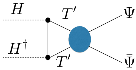
Figure 2: A loop induced contribution to $Z-b-b$ coupling, utilizing strong dynamics to couple heavy top partners to SM third generation fermions.

Note, additional corrections to the $Z\bar{b}b$ coupling can be induced through operators such as $(HQ_{L})^{\dagger}\not{D}(HQ_{L})$. Such operators can be generated by integrating out heavy resonances of $b_{R}$. However, these contributions are proportional to $y_{b}^{2}$ and thus negligible.

In theories of compositeness/strong dynamics, the oblique parameters $S$ and $T$ Peskin and Takeuchi (1992, 1990) often provide an important constraint. However, in our theory, where the Higgs remains elementary, these constraints are weakened.

The relevant operators can be written as Grinstein and Wise (1991); Han and Skiba (2005)

$${\mathcal{O}}_{S} = c_{S}(H^{\dagger}\tau^{a}H)W^{a}_{\mu\nu}B^{\mu\nu},$$ (13)

$${\mathcal{O}}_{T} = c_{T}|H^{\dagger}D_{\mu}H|^{2},$$ (14)

with

$$c_{S} = \frac{1}{4sc}\frac{\alpha}{v^{2}}S,$$ (15)

$$c_{T} = -2\frac{\alpha}{v^{2}}T.$$ (16)

In this case, there are constraints both directly on the compositeness scale $\Lambda_{C}$ as well as on the scale $f$. The contribution directly constraining $\Lambda_{C}$ arises from integrating out heavy states such as the $T^{\prime}$ (there is a box diagram). The second contribution comes from coupling Higgs bosons to the $T^{\prime}$, and then using the four-fermion verxtex involving four $T^{\prime}$’s suppressed by $f^{2}$. For $c_{T}$, we have contributions

$$c_{T}=\frac{\eta_{T}^{\Lambda}N_{c}y_{t}^{4}}{16\pi^{2}\Lambda_{C}^{2}},\,\,\frac{\eta_{T}^{f}N_{c}^{2}y_{t}^{4}}{(16\pi^{2})^{2}f^{2}}.$$ (17)

These contributions are equal for $\Lambda_{C}=4\pi f$ as assumed in NDA. For the $S$ parameter, we have:

$$c_{S}=\frac{\eta_{S}^{\Lambda}N_{c}y_{t}^{2}gg^{\prime}}{16\pi^{2}\Lambda_{C}^{2}},\,\,\frac{\eta_{S}^{f}N_{c}^{2}y_{t}^{2}gg^{\prime}}{(16\pi^{2})^{2}f^{2}},$$ (18)

which are again equal under the NDA assumption. Imposing approximate 2$\sigma$ bounds $S<0.16$ and $T<0.22$, we find $S$ implies $\Lambda_{C}>\sqrt{\eta_{S}^{\Lambda}}$ 1200 GeV, while $T$ implies $\Lambda_{C}>\sqrt{\eta_{T}^{\Lambda}}$ 610 GeV. For the oblique parameters, we expect the bounds directly dependent on $\Lambda_{C}$ to be the strongest constraints, as $\Lambda_{C}<4\pi f$.

VI.2 4-Fermi operators

We now turn to the four-fermion interaction term, i.e.

$${\mathcal{O}}_{4f}=c_{4f}(\bar{\Psi}\gamma^{\mu}\Psi)(\bar{\Psi}\gamma_{\mu}\Psi).$$ (19)

We expect $c_{4f}=\eta_{4f}/f^{2}$, with $\eta_{4f}$ a presumably order one number. Such interactions are introduced, e.g. by the exchange of resonances of the strong dynamics.

It was proposed in Lillie et al. (2008); Kumar et al. (2009) that the search in four top channels at the LHC could impose strong constraints on composite top scenarios. See also Fabbrichesi et al. (2014); Englert et al. (2014); Pomarol and Serra (2008). Such a study has been carried out by ATLAS at 13 TeV with 3.2 fb^-1 data The ATLAS Collaboration (2016). $c_{4f}$ is constrained at the 95% confidence level as

$$c_{4f}<\frac{5}{\rm{TeV}^{2}},$$ (20)

which implies $f>\sqrt{\eta_{4f}}$ 450 GeV. Depending on the precise value of $\eta_{4f}$, this constraint can either be weaker or stronger than the indirect constraints arising from $Z\rightarrow b\bar{b}$ discussed in the previous section ($f>\sqrt{\eta_{b}^{loop}}$ 410 GeV). Importantly, we expect the bounds on this operator to improve dramatically with new LHC data.

It may be possible that the rank of strongly coupled group, i.e. $N$, or the representations of partons under the new strong dynamics may give an argument for an effective suppression of $c_{4f}$. To flesh out how this might occur, we first review an example from QCD, and then contrast how things would differ with more exotic representations. We build our way up to derive the $N$ counting for a baryon-baryon interaction mediated by pion exchange. The interaction between a pion and partonic quarks scales as $\frac{1}{\sqrt{N}}$: the two point correlation function between two pions has an $N$ enhancement, due to a closed color loop, and $\frac{1}{\sqrt{N}}$ appears in the pion-quark interaction vertex after proper normalization. The interaction between a baryon (formed by $N$ quarks in fundamental representation) and a pion scales as $\sqrt{N}$: baryons carry $N$ colored lines, allowing $N$ ways to insert the pion-quark vertex into a baryon. When combined with the factor of $\frac{1}{\sqrt{N}}$ from the pion-quark vertex, the baryon-pion interaction scales as $\sqrt{N}$. This implies that the baryon-baryon interaction mediated by pion exchange scales as $N^{0}$ because there is only one way to insert the pion into a second baryon after the color has been fixed via the choice on the first baryon.

This discussion relies on the assumption that the baryon is formed by $N$ quarks which are in the fundamental representation of $SU(N)$. If the partons transform in a more complicated representation, then the $N$-scaling differs. For example, if the new strong dynamics is given by $SU(6)$, then the top quark could conceivably be comprised of three quarks, $\psi_{1,2,3}$, transforming as 6, 15, 20 representations, respectively. Although color-singlet mesons still take the form $M_{i}\sim\bar{\psi}_{i}\psi_{i}$, the meson-parton vertex now scales as $(\frac{1}{\sqrt{N}})^{i}$. This is because the $i^{\rm{th}}$ parton carries $i$ color indices and there are $i$ closed color lines when computing the two point correlation functions of these mesons, There is no compensating factor, as there is only one way to insert a meson to a baryon when computing the interaction mediated by these mesons: the meson-parton vertex vanishes if the meson is composed by a different species of parton. So, it seems plausible that interactions among baryons may be suppressed if the partons transform in complicated representations. Of course, whether that obtains is a model-dependent question.

VI.3 Flavor/CP constraints

VI.3.1 Flavor constraints

Flavor is a concern in models where the third generation quark is composite. As discussed in Georgi et al. (1995), once the fermions in Eq. (7), (8) and (19) are rotated to the mass basis, severe flavor problems may result. Let us explicitly illustrate how flavor changing processes are introduced. The mixing between the first two generations and the third generation quarks can be characterized by the following approximate rotations, which take quarks from the interaction ($I$) basis to the mass ($M$) basis:

$$t_{L/R,I} \approx \theta_{L/R}^{u}u_{L/R,M}+\theta_{L/R}^{c}c_{L/R,M}+t_{L/R,M},$$

$$b_{L/R,I} \approx \theta_{L/R}^{d}d_{L/R,M}+\theta_{L/R}^{s}s_{L/R,M}+b_{L/R,M}.$$ (21)

In our scenario, only operators involving the third generation are directly generated by the strong dynamics. This argues the operators Eq. (7), (8) and (19) naturally only involve third generation partons in the interaction basis.

Operators connecting the first two generations with the partons forming the third generation may be generated at a higher scale. Indeed, the observed CKM matrix indicates that the mixing between the third generation and the first two generations is small (but not zero). Non-renormalizable operators above confinement scale can be responsible for this mixing:

$$\frac{1}{\Lambda_{\textrm{mixing}}^{3(m-1)/2}}H\psi_{s}^{m}\psi_{1,2},$$ (22)

where $\psi_{s}$ generically labels partons of the third generation quarks in strong dynamics, and we assumed there are $m$ partons combined together to form a third generation quark. $\psi_{1,2}$ stands for the first two generation elementary quarks. $\Lambda_{\textrm{mixing}}$ is a scale higher than $\Lambda_{C}$ where the mixing is generated. Passing through the confinement scale, $\psi_{s}^{m}$ becomes a single composite fermion in the IR (a third generation quark), and the high dimension operators become effective marginal operators,

$$\frac{1}{\Lambda_{\textrm{mixing}}^{3(m-1)/2}}H\psi_{s}^{m}\psi_{1,2}\rightarrow\bigg{(}\frac{\Lambda_{C}}{\Lambda_{\textrm{mixing}}}\bigg{)}^{3(m-1)/2}H\psi_{3}\psi_{1,2}.$$ (23)

Such operators generate the mixing between the third generation quarks and the first two generations. This mixing is dangerous when combined with the operators generated by strong dynamics that we now discuss.

There are four independent classes of operators relevant to flavor changing processes:

$$\mathcal{O}_{F1} = \frac{e^{2}}{\Lambda_{C}^{2}}(\bar{\Psi}_{L/R}\gamma^{\mu}\Psi_{L/R})(\bar{l}\gamma^{\mu}l),$$

$$\mathcal{O}_{F2} = e\frac{m_{\Psi}}{\Lambda_{C}^{2}}F_{\mu\nu}(\bar{\Psi}_{L/R}\sigma^{\mu\nu}\Psi_{R/L}),$$

$$\mathcal{O}_{F3} = \frac{1}{f^{2}}(\bar{\Psi}\gamma^{\mu}\Psi)(\bar{\Psi}\gamma_{\mu}\Psi),$$

$$\mathcal{O}_{F4} = \frac{1}{16\pi^{2}f^{2}}(H^{\dagger}D_{\mu}H)(\bar{\Psi}\gamma^{\mu}\Psi).$$ (24)

Prior to mixing, the $\Psi$ are third generation fermions. The first two classes of operators induce processes with $\Delta F=1$ such as $b\rightarrow s\gamma$ or $b\rightarrow s\ell^{+}\ell^{-}$. The first operator in Eq. (VI.3.1) is related to the operator with photon field strength by equations of motion, i.e. $e\frac{i}{\Lambda^{2}}F_{\mu\nu}\bar{\Psi}_{L/R}D^{\mu}\gamma^{\nu}\Psi_{L/R}$. The last operator is analogous to the operator discussed in the context of $Z\rightarrow b\bar{b}$, but here (after mixing) we allow for flavor dependence on the coupling. For most processes, under the assumption that $4\pi f>\Lambda_{C}$ the effect of this operator will be subdominant to the effects of the other operators.

The mixing angles in Eq. (VI.3.1) are not arbitrary, since they are related to elements in the CKM matrix. Under the approximation that all $\theta$’s are small, these mixing parameters can be related to the elements in CKM matrix at leading order as

$$|\theta_{L}^{d*}+\theta_{L}^{u}| \simeq |V_{ub}|,$$

$$|\theta_{L}^{s*}+\theta_{L}^{c}| \simeq |V_{cb}|,$$ (25)

where $|V_{cb}|\simeq 0.04$ and $|V_{ub}|\simeq 0.004$. The mixing angles of left-handed quarks for both up and down-type quarks cannot be simultaneously be taken arbitrarily small. As we will see, the constraints arising from FCNC involving $b$ quarks are particularly strong. It is therefore advantageous to induce the quark mixing mainly via the up-type Yukawas ($\theta_{L}^{d}\simeq\theta_{R}^{d}\simeq 0$). Making this choice, the dominant constraints come from D-meson mixing.

Before discussing this in detail, let us first emphasize the danger of allowing appreciable mixing in the down sector. The constraints on B-meson oscillations have been studied in Calibbi et al. (2012); Altmannshofer and Straub (2015), and we will reinterpret their results accordingly. We first consider the operators with all left-handed fermions, i.e. $\frac{1}{f^{2}}(\bar{\Psi}_{L}\gamma^{\mu}\Psi_{L})(\bar{\Psi}_{L}\gamma_{\mu}\Psi_{L})$. The constraints from $B$-meson oscillation can be derived as

$$f \!\mathrel{\hbox{\hbox to0.0pt{\lower 2.36806pt\hbox{$\sim$}\hss} \kern-3.39996pt\raise 1.72218pt\hbox{$>$}}} 2.3\,\bigl{(}\frac{\theta_{L}^{d}}{0.004}\bigr{)}\ \textrm{TeV}\ \ \ \ \ B_{d}\ \textrm{oscillation,}$$

$$f \!\mathrel{\hbox{\hbox to0.0pt{\lower 2.36806pt\hbox{$\sim$}\hss} \kern-3.39996pt\raise 1.72218pt\hbox{$>$}}} 10\,\bigl{(}\frac{\theta_{L}^{s}}{0.04}\bigr{)}\ \textrm{TeV}\ \ \ \ \ B_{s}\ \textrm{oscillation.}$$ (26)

We have normalized the angles to the relevant CKM mixings. If left-handed and right-handed mixing angles are comparable to each other, the strongest constraints are imposed to mixed chirality operators, i.e. $\frac{1}{f^{2}}(\bar{\Psi}_{L}\Psi_{R})(\bar{\Psi}_{L}\Psi_{R})$:

$$f \!\mathrel{\hbox{\hbox to0.0pt{\lower 2.36806pt\hbox{$\sim$}\hss} \kern-3.39996pt\raise 1.72218pt\hbox{$>$}}} 6.2\sqrt{\frac{\theta_{L}^{d}}{0.004}}\sqrt{\frac{\theta_{R}^{d}}{0.004}}\ \textrm{TeV}\ \ \ \ \ B_{d}\ \textrm{oscillation,}$$

$$f \!\mathrel{\hbox{\hbox to0.0pt{\lower 2.36806pt\hbox{$\sim$}\hss} \kern-3.39996pt\raise 1.72218pt\hbox{$>$}}} 26\sqrt{\frac{\theta_{L}^{s}}{0.04}}\sqrt{\frac{\theta_{R}^{s}}{0.04}}\ \textrm{TeV}\ \ \ \ \ B_{s}\ \textrm{oscillation.}$$ (27)

The normalization of the $\theta_{R}$ is somewhat arbitrary, as it is not directly related to a CKM angle. Here, we have considered the constraint on the real part of the operator; the constraint on the imaginary part is modestly ($\sim$ factor 2) stronger.

In the Appendix, we briefly review other bounds coming from down-type mixing, but motivated by the severity of the above bounds, we will suppose that quark mixing is generated via the up-type quarks.

$\Delta C=2$ processes, i.e. D-meson oscillation, are induced from $\mathcal{O}_{F3}$ in Eq. (VI.3.1): the effective operators are proportional to $(\theta_{L/R}^{c}\theta_{L/R}^{u})^{2}$. While the operator in Eq. (VI.3.1) containing all left-handed top quarks is necessarily real, following the rotation to the mass basis, a contribution to CP-violation in the charm sector appears. This imposes a particularly stringent constraint, as the Standard Model contribution is expected to be very small. Indeed, when all quark mixing arises from the left-handed up quarks, not only are $\theta_{L}^{u/c}$ are responsible for generation of $|V_{ub}|$ and $|V_{cb}|$ in CKM matrix, the phases of $\theta_{L}^{u/c}$ are related to the physical phase in CKM matrix.

Let us discuss this constraint in some detail: CP-violation in the D-meson system has been constrained via a variety of final states. Particularly relevant are: $D^{0}\rightarrow K^{+}\pi^{-}$, $D^{0}\rightarrow K^{+}K^{-}$ and $D^{0}\rightarrow\pi^{+}\pi^{-}$. The strongest constraints typically come from $D^{0}\rightarrow K^{+}\pi^{-}$, but this statement depends on whether there is direct CP violation (CPV) in doubly Cabbibo suppressed ($c\rightarrow du\bar{s}$) decays. If present, this additional free parameter can “soak-up” CPV in the mixing in $D^{0}\rightarrow K^{+}\pi^{-}$, via a cancellation. In our scenario, however, we expect this direct CPV to be small, so the stronger constraints apply Heavy Flavor Averaging Group .

Before presenting detailed numbers, we show the CP violation in our scenario is invariant under the reparameterization of the CKM matrix. As an example, consider the $D^{0}\rightarrow\pi^{+}\pi^{-}$ channel. Since we have set the mixings in down-type sector to vanish, we have $\theta_{L}^{u}=V_{ub}^{*}$ and $\theta_{L}^{c}=V_{cb}^{*}$. Staring with $\mathcal{O}_{F3}$ in the interaction basis, we rotate the quarks into mass basis, and find

$$c_{\mathcal{O}_{F3}}(V_{ub}^{*}V_{cb})(\bar{c}_{L}\gamma^{\mu}u_{L})(\bar{c}_{L}\gamma_{\mu}u_{L}).$$ (28)

This operator induces mixing between $D^{0}$ and $\bar{D}^{0}$. Including the D-meson decay in the $\pi\pi$ channel we find CPV proportional to $\textrm{Im}[(V_{ub}^{*}V_{cb})^{2}(V_{cd}^{*}V_{ud})^{2}]$, which is CKM reparameterization invariant Jarlskog (1985). For simplicity, we choose the standard parametrization where the CP-violating phase is primarily moved to $V_{td}$ and $V_{ub}$. From Heavy Flavor Averaging Group , we choose CP violating parameters within the 2$\sigma$ allowed region, i.e. $x_{12}=0.4\%$ and $\phi_{12}=5^{\circ}$. This translates to

$$f\!\mathrel{\hbox{\hbox to0.0pt{\lower 2.36806pt\hbox{$\sim$}\hss} \kern-3.39996pt\raise 1.72218pt\hbox{$>$}}}\sqrt{\eta_{4f}}\,810\,\textrm{GeV}.$$ (29)

We have included the RG running on the operator following Golowich et al. (2009). This is the strongest constraint on $f$ from indirect measurements. A $40\%$ tuning (cancellation) among the four-fermion operators (perhaps via a tiny mixing amongst the right-handed up quarks) would reduce this constraint below the direct constraint on $\mathcal{O}_{F3}$ from 4-top production at the LHC, $f>450$ GeV.

The mixing in Eq. (VI.3.1) also induces $\Delta C=1$ rare D-meson decays, such as $D^{+}\rightarrow\pi^{+}+\mu^{+}+\mu^{-}$ and $D\rightarrow\mu^{+}\mu^{-}$. The effective operators after rotation are proportional to $(\theta_{L/R}^{c}\theta_{L/R}^{u})$. However, The presence of large long-distance contributions to these decays weaken these constraints, and following Fajfer and Košnik (2015), we find these constraints are subdominant to those derived from mixing.

We briefly note the potential importance of a dimension 6 operator beyond those considered in Eq. (VI.3.1) that is relevant independent of how quark mixing is introduced:

$$i(H^{c{\dagger}}D^{\mu}H)(\bar{t}_{R}\gamma_{\mu}b_{R}).$$ (30)

This operator can induce a coupling between W boson and right-handed top/bottom quarks and has been studied in the context of composite Higgs models in Vignaroli (2012). Because the SM contribution to $b\rightarrow s\gamma$ suffers from helicity suppression, i.e. proportional to $m_{b}$, coming from the mass insertion on the external leg. If the operator in Eq. (30) is present, the mass insertion is not required anymore. Further, the SM contribution is loop suppressed, so even a fairly small coefficient in front of this operator may induce a too-large contribution to $b\rightarrow s\gamma$. Fortunately, in our scenario the coefficient is expected to be suppressed by $y_{b}$. Consider the limit where $y_{b}$ is set to zero: one may assign a conserved quantum number to $b_{R}$. If this is respected by strong dynamics, the bottom Yukawa coupling is the only interaction which violates this $b_{R}$ number. Thus the coefficient in Eq. (30) has to be proportional to $y_{b}$. Similarly, $y_{t}$ should also appear in the coefficient, and the operator can be written as

$$i\frac{y_{t}y_{b}\eta_{Wtb}}{\Lambda_{C}^{2}}(H^{c{\dagger}}D^{\mu}H)(\bar{t}_{R}\gamma_{\mu}b_{R}).$$ (31)

Applying the constraints from $b\rightarrow s\gamma$, we have

$$\Lambda_{C}\!\mathrel{\hbox{\hbox to0.0pt{\lower 2.36806pt\hbox{$\sim$}\hss} \kern-3.39996pt\raise 1.72218pt\hbox{$>$}}}\sqrt{\eta_{Wtb}}\,930\,\textrm{GeV}.$$ (32)

At last, the electric dipole operator (EDM) of top quarks can also be constrained since it contributes to neutron EDM at low energy Kamenik et al. (2012). Prior to electroweak symmetry breaking, these operators can be written as dimension 6 operators:

$$\frac{c_{EDM}g_{i}}{\Lambda_{C}^{2}}\bar{Q}H\sigma^{\mu\nu}UF^{i}_{\mu\nu},$$ (33)

where $i$ stands for SM gauge groups. $F^{i}_{\mu\nu}$ is the field strength of the $i$th group and its gauge index is contracted with the corresponding generator which is implicitly included. The bound on the neutron EDM requires $\textrm{Im}(\Lambda_{C}/\sqrt{c_{EDM}})>4.7\ \textrm{TeV}$. Thus if $\Lambda_{C}$ is 1$\sim$2 TeV, for $c_{EDM}=1$, one needs a mild suppression of CP violating phases in the strongly coupled sector $\phi_{CP}\!\mathrel{\hbox{\hbox to0.0pt{\lower 2.36806pt\hbox{$\sim$}\hss} \kern-3.39996pt\raise 1.72218pt\hbox{$<$}}}0.1$.

VI.4 Mixing between elementary and composite degrees of freedom

The discussion on phenomenological constraints so far ignores the possible mixing between elementary degrees of freedom and composite degrees of freedom. In this section, we present a general analysis and show that the mixing generically does not introduce stronger constraints.

First, $\psi_{L}$ and $\psi_{R}$ can also form a composite scalar, $\Phi_{H}$, with quantum numbers identical to those of the SM Higgs boson. In the present set-up $\Phi_{H}$ is not a pseudo-Nambu Goldstone boson, so its (unprotected) mass is expected to be around confinement scale: $m_{\Phi_{H}}\sim\Lambda_{C}$. The elementary SM Higgs can mix with $\Phi_{H}$. While the mixing cannot be calculated in a precise way, we will argue that expected effects induced by such mixing are comparable or smaller than those enumerated from direct couplings to the elementary Higgs boson.

Although we cannot rule out the possibility of a “tree-level” bare mixing directly present between the elementary Higgs boson and the composite state, we try to estimate its natural size by calculating the loop contribution to this mixing arising from integrating out heavy resonances. The loop contribution can be estimated by integrating out heavy resonance modes from strong dynamics which couple to both Higgs and $\Phi_{H}$. For example, integrating out the excited state of top quark induces a mixing term in Lagrangian as $\mathscr{L}\sim\frac{N_{c}y_{t}g_{*}}{16\pi^{2}\sqrt{N}}\Lambda_{C}^{2}H\Phi_{H}$. For a composite state with mass $\Lambda_{C}$, the mixing angle be estimated to be $\sim\frac{N_{c}y_{t}g_{*}}{16\pi^{2}\sqrt{N}}$. As studied in previous sections, $g_{*}$ is expected to be smaller or comparable to $4\pi$. Thus, with a reasonable choice of $N$, the mixing can be easily smaller than $10\%$ and modifications of Higgs boson properties due to this mixing should be consistent with present measurements.

Higher dimension operators containing $\Phi_{H}$ suffer a smaller effective suppression scale than those operators containing the $H$ directly as $\Phi_{H}$ has strong couplings to other composite states. These operators containing $\Phi_{H}$ will generate operators with $H$ once we account for the above mixing. One might worry that this might induce the dominant contribution to precision electroweak observables, but the mixing compensates for the would-be smaller suppression scale, and these induced operators are expected to be subdominant. To see this, consider operators differ by one power of $H$ and $\Phi_{H}$. They can be written as $\frac{y_{t}H}{\Lambda_{C}}\mathcal{O}$ and $\frac{g_{*}\Phi_{H}}{\sqrt{N}\Lambda_{C}}\mathcal{O}$. Performing the rotation from $\Phi_{H}$ to $H$, the second operator can induces $\frac{g_{*}^{2}y_{t}N_{C}}{16\pi^{2}N\Lambda_{C}}H\mathcal{O}$. So, effects induced from $\frac{g_{*}\Phi_{H}}{\Lambda_{C}}\mathcal{O}$ are comparable or smaller than those from $\frac{y_{t}H}{\Lambda_{C}}\mathcal{O}$, since $g_{*}<4\pi$, especially when $N$ is large. This can be generalized to operators involving an arbitrary number of Higgs fields.

Furthermore, our lighter Higgs boson is mainly elementary. Thus the quartic coupling of the Higgs boson is a free parameter, and there is no expectation that it must be completely generated radiatively (as is the case in composite Higgs models). One may be worried whether the quartic coupling induced by mixing through heavy composite Higgs states would be too large and thus a fine-tuning would be needed to achieve a small value. However, the induced quartic coupling is rendered sufficiently small by the small mixing, thus no additional fine-tuning is needed here. Additional contributions to the Higgs boson quartic can be induced after integrating out heavy resonances. For example, integrating out $T^{\prime}$ (through a box diagram) can induce a correction to $\lambda_{H}$ around $N_{c}y_{t}^{4}/16\pi^{2}$, which is also subdominant to the observed value. Thus one does not need to worry about additional fine tuning induced through Higgs quartic term.

Heavy composite vector bosons, transforming in adjoint representation of SM gauge group, can be formed by the partons of the strong dynamics. These vector bosons can mix with SM gauge bosons. After redefinition of the SM gauge boson, such mixing will induce a small coupling between SM charged particles to composite vector bosons. Similar to the $H$ and $\Phi_{H}$ mixing, the the mixing between gauge boson and heavy composite vector fields can be estimated as $\epsilon\sim\frac{g_{i}g_{*}N_{C}}{16\pi^{2}\sqrt{N}}$. After a field redefinition, the coupling between particles charged under the SM and heavy vectors is $\frac{g_{i}^{2}g_{*}N_{C}}{16\pi^{2}\sqrt{N}}$. Integrating out these heavy vectors, introduces dimension 6 operators with Wilsonian coefficients as $\frac{g_{i}^{4}g_{*}^{2}N_{C}^{2}}{(16\pi^{2})^{2}N\Lambda_{C}^{2}}\mathcal{O}_{6}$. For $SU(3)_{c}$, these operators are 4-quark interactions. Given $\Lambda_{C}$ higher than TeV, these operators are far from being probed. On the other hand, the mixing between $SU(2)_{L}$ gauge boson and heavy vector can be important since that can induce additional contributions to operators like $Z\bar{b}b$ coupling or $T$-parameter, for example. However, these additional contributions are small compared to the ones we have discussed in the previous section as long as $\frac{g_{i}^{4}g_{*}^{2}N_{C}^{2}}{16\pi^{2}N}<1$.

VI.5 Summary on phenomenological constraints

Before closing this section, let us summarize the most stringent constraints in our scenario (all at 95% confidence):

$\bullet$ The $S$-parameter imposes the strongest direct constraint on $\Lambda_{C}\!\mathrel{\hbox{\hbox to0.0pt{\lower 2.36806pt\hbox{$\sim$}\hss} \kern-3.39996pt\raise 1.72218pt\hbox{$>$}}}\sqrt{\eta_{S}^{\Lambda}}\ 1200\ \textrm{GeV}$.

$\bullet$ $Z\rightarrow b\bar{b}$ constrains $f\!\mathrel{\hbox{\hbox to0.0pt{\lower 2.36806pt\hbox{$\sim$}\hss} \kern-3.39996pt\raise 1.72218pt\hbox{$>$}}}\sqrt{\eta_{b}^{loop}}\ 410$ GeV.

$\bullet$ The LHC 4-top searches directly constrain $f\!\mathrel{\hbox{\hbox to0.0pt{\lower 2.36806pt\hbox{$\sim$}\hss} \kern-3.39996pt\raise 1.72218pt\hbox{$>$}}}\sqrt{\eta_{4f}}\ 450$ GeV.

$\bullet$ Assuming all mixing is from up-type sector, CP violation in D-meson mixing gives the strongest constraint on $f\!\mathrel{\hbox{\hbox to0.0pt{\lower 2.36806pt\hbox{$\sim$}\hss} \kern-3.39996pt\raise 1.72218pt\hbox{$>$}}}\sqrt{\eta_{4f}}\ 810$ GeV. A $40\%$ cancellation among operators can make it comparable to those from direct 4-top LHC searches.

The first constraint directly applies to $\Lambda_{C}$, all other constraints are imposed on the suppression scale of 4-fermion operators induced by strong dynamics. In NDA, $\Lambda_{C}\simeq 4\pi f$, but there are two subtleties when translating the constraints on $f$ to $\Lambda_{C}$. First, it depends on the choice of strong coupling $g_{\ast}$. Second, the representations under $SU(N)$ of the top’s partons may introduce non-trivial $N$-dependence to 4-fermion operators. With these subtleties in mind, we conclude the current constraints on composite scale are $\Lambda_{C}\!\mathrel{\hbox{\hbox to0.0pt{\lower 2.36806pt\hbox{$\sim$}\hss} \kern-3.39996pt\raise 1.72218pt\hbox{$>$}}}$ TeV – though if the NDA estimate were to hold this would be closer to 4 TeV (8 TeV from mixing in the charm sector). If $\Lambda_{\psi}$ is not too large and $\Lambda_{C}\approx$ TeV, the fine tuning in our scenario is a few percent.

VII Comments on Collider Signatures

At a hadron collider such as the LHC, the colored parton(s) comprising $\phi_{c}$ can be directly produced. If the collision energy of a particular event is below $\Lambda_{C}$, top and bottom quarks are the only light degrees of freedom energetically accessible. Colored parton production is effectively the production of the third generation quarks. One can in principle study differential distributions, such as $d\sigma/dm_{\bar{t}t}$ and $d\sigma/dm_{\bar{b}b}$. The third generation quarks’ couplings to gluons will acquire a from factor, and deviations in the top quark production might be expected as the center of mass energy approaches $\Lambda_{C}$. However, uncertainty in modeling of SM top production is a challenge. More promising are searches for 4-top production as outlined in the previous section.

On the other hand, if the collision energy is above $\Lambda_{C}$, colored partons in composite top can be produced as elementary particle, and we start to directly probe new physics of $SU(N)$ group.

First of all, we expect several heavy composite states whose masses are about $\Lambda_{C}$, such as a $\rho^{\prime}$. These particles may or may not be charged under $SU(3)_{C}$, depending on their parton content. The most straightforward way to look for such particles may be through resonance searches. For example, one can look for the $\rho^{\prime}$ through ditop resonance search. Such analysis has been carried out in CMS Khachatryan et al. (2016). They have searched for a Kaluza-Klein gluon with width $\approx 15\%$ of its mass, and find a limit of $\approx 2.3$ TeV. We would expect there might be color octet resonances in this scenario as well. However, as we will see, the both the production rate and width can differ from the target of the CMS search, thus induce a weaker constraint.

In order to compare the production cross section, we consider two possible production channels. First, as discussed in Sec. VI.4, a coupling between light quarks and heavy vector resonance can be introduced through mixing with SM gluon. After field redefinition, the coupling is about $\frac{g_{S}^{2}g_{*}N_{C}}{16\pi^{2}\sqrt{N}}$. For comparison, in the CMS search, the couplings of KK-gluon are assumed to be about 0.2$g_{S}$ for most quarks and $g_{S}$ for $t_{R}$. If $g_{*}$ is mildly smaller than $4\pi$, with a generic choice of $N$, the production cross section of $\rho^{\prime}$ can be comparable to KK-gluon considered in CMS search.

Production via gluon fusion is also possible in principle. If the $\rho^{\prime}$ is somewhat smaller than $\Lambda_{C}$, a rough estimate of gluon fusion production can be obtained by integrating out the colored states of the strong dynamics that are present above $\Lambda_{C}$. Alternately, if the mass of the $\rho^{\prime}$ is somewhat larger than $\Lambda_{C}$, one can consider the production of the colored partons, and estimate the production of the $\rho^{\prime}$ by considering the overlap of the partons in the $\rho^{\prime}$ bound state. Either estimate yields a production rate subdominant to the production via the quarks discussed above, so we can expect $\rho^{\prime}$ production to be comparable or smaller to that of the CMS KK gluon benchmark. Moreover, for this search to be effective, the width of the heavy resonance cannot be too large, or else the features of a resonance are smeared in SM background (though with precise modeling of $\bar{t}{t}$ production, it might be possible to observe a broad excess in the future). This likely occurs here due to the strong $SU(N)$ interactions. Thus, direct resonance search constraints may be comparable to, and quite possibly weaker than the indirect bounds as found in Sec. VI. If the resonance happens to be somewhat narrow, resonance searches of this type could indeed be a useful way to test this scenario, but the narrowness is not guaranteed, as we now discuss.

One may ask whether a large width for these heavy resonances is in contradiction with the desire to have $\Lambda_{C}$ and $f$ separated by a factor smaller than $4\pi$. (Recall, the strongest bounds are on $f$, so reducing this factor will reduce the fine-tuning in our model, which depends directly on $\Lambda_{C}$.) Alternately, one may wonder whether requiring $1/N$ suppression in operators suppressed by $1/f^{2}$ (see discussion in Sec. VI.2) will always lead to a small decay width. We present a simple estimate to show that a modest suppression of these operators beyond $1/f^{2}$ is consistent with a large decay width (e.g. if $N$ is not too large). For simplicity, we assume the only light composite particles are the top and bottom. If there were additional (possibly SM neutral) light composites, this could further increase the decay width heavy resonances.

First, assume the $SU(3)_{c}$ colored parton is in the fundamental representation of $SU(N)$, while the other partons in the composite top are in different representations. Similar to the argument for pion interactions, the coupling between a heavy resonance and colored parton scales as $g_{*}/\sqrt{N}$. Consider the case where the heavy resonance is a vector meson $\rho^{\prime}$ which is an octet of $SU(3)_{C}$ (analogous to the KK gluon). Since there is only one way to contract the two colored partons of this composite state with the partons in the third generation fermions, its coupling is

$$\mathscr{L}\supset i\frac{g_{*}}{\sqrt{N}}\rho^{\prime}_{\mu}\bar{\Psi}\gamma^{\mu}\Psi.$$ (34)

Integrating out the $\rho^{\prime}$ generates the 4-fermion operator at low energy,

$$\mathscr{L}\supset\frac{g_{*}^{2}}{2N}\frac{1}{\Lambda_{C}^{2}}(\bar{\Psi}\gamma^{\mu}\Psi)(\bar{\Psi}\gamma_{\mu}\Psi).$$ (35)

Here we have set $m_{\rho^{\prime}}\simeq\Lambda_{C}$. One can further calculate the $\rho^{\prime}$ width induced by this coupling at tree level. Including both top and bottom decay channels, we get

$$\Gamma=\frac{g_{\ast}^{2}}{12\pi N}M_{\rho^{\prime}}.$$ (36)

To evade the constraints from ditop resonance searches, we require the width of $\rho^{\prime}$ be the same order as its mass $\Gamma_{\rho^{\prime}}=c\ M_{\rho^{\prime}}$ where $c\sim 1$. The 4-fermion operator induced by integrating out $\rho^{\prime}$, Eq. (35), can be rewritten as

$$\mathscr{L}\supset\frac{6\pi c}{\Lambda_{C}^{2}}(\bar{\Psi}\gamma^{\mu}\Psi)(\bar{\Psi}\gamma_{\mu}\Psi).$$ (37)

At least in this simple example, we see it is consistent to simultaneously have a wide $\rho^{\prime}$ and a suppression scale modestly larger than $\frac{\Lambda_{C}}{4\pi}$ in the 4-fermion interaction it induces. If the heavy resonances are very wide, they are similar to the $\sigma$ particle in QCD, and it could be highly non-trivial to find these particles at a hadron collider.

We also expect excited states of the new composite top quark, i.e. $T^{\prime}$. Again, these heavy states are expected near $\Lambda_{C}$, and their widths can be large. We expect the,$\rho^{\prime}$, which couples strongly to $T^{\prime}$, to have a comparable mass. If $\rho^{\prime}$ is lighter than the excited top state, $T^{\prime}$ should dominantly decay to $\rho^{\prime}+t$ and consequently lead to $3t$ or $t+2b$ in its final states. Even if $\rho^{\prime}$ is a little heavier than $T^{\prime}$, due to its large coupling to $T^{\prime}$, the 3-body decay channel through off-shell $\rho^{\prime}$ can still be comparable or even larger than electroweak decay channels, such as $t+Z$, $b+W$ and $t+H$ where $W$ and $Z$ are mainly in their longitudinal modes. The other possible decay channel is through $t+g$. The current constraints from those channels are around 800 GeV Chatrchyan et al. (2014); Khachatryan et al. (2015); ATL (2016); collaboration (2016), thus weaker than those from EWPTs and flavor/CP measurements discussed above. Furthermore, the low energy spectrum from $SU(N)$ strong dynamics may not be limited to top and bottom. If there are other light composite states, which may well be SM neutral, their existence can change collider signatures dramatically.

This is very different from the fermionic top partner $T$, in composite Higgs models. In those models, $T$’s have masses much lower than confinement scale, thus there are no additional states from strong dynamics to which they can decay. Thus, it is more certain top partners in these models will decay as $t+Z$, $b+W$ and $t+H$ (though it is possible that there might be additional light scalars in the spectrum Kearney et al. (2013)). It is also interesting to note that the $T^{\prime}$ of our scenario could conceivably be observed but would not be responsible for the cancellation of the ultimate quadratic divergence. Rather they could be partially responsible for the form factor that cuts off the first divergence shown in Eq. (1).

In summary, there are multiple reasons that new particles might be difficult to see at colliders. First, some resonances may be difficult to find due to their likely width, e.g. the $\rho^{\prime}$ and, potentially, excitations of the top. The states ultimately responsible for the cancellation of the final quadratic divergence near $\Lambda_{\psi}$, on the other hand, would not necessarily be expected to be wide. For example, in the case of a SUSY UV completion, a stop could decay to a Bino and top only via a weak coupling. Nevertheless, searches for these particle are also difficult due to the screening effect.

At sufficiently high energies additional interesting phenomena may appear. If a pair of $SU(3)_{c}$ colored partons are produced, each with energy much higher than $\Lambda_{C}$, they will produce $SU(N)$ singlets via hadronization. It is possible that multiple third generation quarks will be produced in the final states. The hadron multiplicity has been studied in detail in the context of SM QCD. For $e^{+}e^{-}$ annihilation at center of mass energy $\sqrt{s}$, the average multiplicity of any hadron species from QCD hadronization can be approximated as Webber (1994)

$$\langle n(s)\rangle\sim exp\bigg{\{}\frac{1}{b}\sqrt{\frac{2N_{c}}{\pi\alpha_{s}(s)}}\bigg{\}},$$ (38)

where $b$ is related to the beta function of strong coupling as $\beta(\alpha_{s})=-b\alpha_{s}^{2}+...$. We expect a similar expression to control the hadronization of the $SU(N)$ group. The value of $b$ in for the new gauge group depends on the details of UV completion. If the running of $SU(N)$ is not too fast, i.e. $b$ is not too large, there can be an enhancement of top and bottom quark multiplicities when the collision energy grows beyond few times $\Lambda_{C}$.

As mentioned earlier, there could also be additional light composite particles beyond the top and bottom. While, if uncolored, direct production of such states is small, they could be produced in hadronization processes, which might change the collider signatures dramatically– for example, giving rise to events with large missing energy if they are stable.

VIII Conclusion

We have explored the possibility that the top quark is composite at the TeV scale, with the Higgs boson coupling to uncolored constituents. Production of colored top partners at hadron colliders can be screened via hardonization effects of the new confining gauge group.

This scenario is likely tuned at the percent level, with particularly strong bounds from EWPT and from flavor/CP physics. The exact strength of these bounds is somewhat model dependent. This scenario should be well tested at the next run of the LHC, where effects should show up in the four top final state. As mentioned, flavor physics represents a strong challenge for this approach, and without careful model building, deviations would have been expected to show up already in the kaon or $B$-meson mixing. When quark mixing arises from the up-type quarks, constraints are more modest, and new physics is expected to arise as CP violation in the $D$-meson system, though cancellations between operators could postpone the appearance of a signal.

This model differs from the related approach of CFT duals of Randall-Sundrum (RS) model building. For example, we have entertained the possibility that new narrow resonances of the strong dynamics are not present, whereas in RS scenarios, these resonances are guaranteed as Kaluza-Klein modes on the AdS side. Their masses and couplings are closely related to the existence of the conformal symmetry and the assumption of large $N$ needed for the weakly coupled gravity dual. Without these assumptions there is no assurance that these states are narrow. In addition, in the RS scenario, flavor originates from a marriage of overlaps of extra-dimensional wave functions and Yukawa couplings. In our scenario, there is no extra-dimensional picture that allow calculability of the top/bottom Yukawa couplings.

There are important differences with respect to traditional composite Higgs (CH) theories as well. In traditional CH models, there is a single scale of strong dynamics. The Higgs boson is light with respect to the scale of strong dynamics due to its pseudo-Goldstone nature. Here, the lightness of the Higgs boson is ultimately ensured by additional physics above our initial (top) compositeness scale. In traditional CH theories, a first signal is often found in colored fermionic partners of the top quark, who ensure that the UV cutoff is $f$, rather than $\Lambda_{C}$. In our theory, these top partners are not present below the confinement scale, which allows their production to be screened. Deviations from precision electroweak observables, precisely because the Higgs boson is elementary, go like $1/\Lambda_{C}$ rather than $1/f$, which allows us to have a lower value of $\Lambda_{C}$. Thus, we do not pay a large fine-tuning price for the absence of top partners in the low-energy effective theory below $\Lambda_{C}$.

The scenario as we have outlined it is truly a “minimal” composite theory in terms of LHC phenomenology. In traditional CH models, it is natural to expect relatively narrow fermionic top partners because their mass is below the confinement scale. In contrast, in our scenario, all heavy particles can be around or above $\Lambda_{C}$, and their widths can be naturally large due to strong coupling and therefore difficult to detect. At present, this theory is not especially less fine-tuned than other CH models – indeed, it is already tuned at the few percent level – but it would explain the absence of resonances into the future. Instead, the likely proof of this theory would come in evidence for anomalous four top production at the LHC, perhaps soon. And if $\Lambda_{C}$ is close to the current experimental bound, collisions in excess of this energy might reveal spectacular signatures, though these depend on the details of the new strong dynamics.

Appendix A Examples of “UV” models and Anomaly cancellation

In this appendix, we write a “partial UV” model which can induce composite third generation quarks. Anomaly cancellation is generically a concern because the $SU(3)_{c}$ and EW charge assignments in our proposal differ from those in SM. In this section, we present two models where cancellations of all gauge anomalies can be achieved and relevant global anomalies are matched. We say that we present a “partial UV” model, because our models include a scalar $\phi_{c}$, which we do not envision as fundamental. Our (admittedly strong) assumption is that whatever additional dynamics gives rise to this scalar does not introduce additional anomalies. This is also the underlying assumption applied in Ref. Abbott and Farhi (1981b).

A.1 The simplest module

The matter content with the simplest setup is written in Table 1. We take the strong group as $SU(N)$. The $SU(N)$ gauge singlets after confinement are identified with SM third generation quarks. More explicitly, $Q_{L,3}^{\alpha}\sim(\phi_{c}\psi_{L}^{\alpha})$ and $t_{R}^{\alpha}/b_{R}^{\alpha}\sim(\phi_{c}^{\dagger}\psi_{R,t/b}^{\alpha})$. In the IR, the theory is assumed to be the SM, so all gauge anomalies are canceled there. In Table. 2, we show anomalies in UV theory. All anomalies can be canceled by taking $Nx=1$.

Particles	$SU(N)$	$SU(3)_{c}$	$SU(2)_{L}$	$U(1)_{Y}$
$\phi_{c}$	$\bar{\square}$	$\square$	$\bullet$	$(\frac{1}{6}-\frac{x}{2})$
$\psi_{L}^{\alpha}$	${\square}$	$\bullet$	$\square$	$\frac{x}{2}$
$\psi_{R,t}^{\alpha}$	$\bar{\square}$	$\bullet$	$\bullet$	$-\frac{1}{2}(x+1)$
$\psi_{R,b}^{\alpha}$	$\bar{\square}$	$\bullet$	$\bullet$	$-\frac{1}{2}(x-1)$

Table 1: The gauge charges of partons in composite third generation quarks.

$U(1)_{Y}$	0	$U(1)_{Y}^{3}$	$\frac{3}{4}(1-Nx)$
$U(1)_{Y}\times SU(2)_{L}^{2}$	$\frac{1}{2}(Nx-1)$	$U(1)_{Y}\times SU(N)^{2}$	0
$SU(3)_{c}^{3}$	0	$SU(N)^{3}$	0

Table 2: The gauge anomalies can be canceled properly in this “partial UV” model by choosing $Nx=1$.

Now, consider t’Hooft global anomaly matching ’t Hooft (1980). When $SU(N)$ becomes strongly coupled, other gauge couplings may be treated as perturbations, and there is an approximate global symmetry: $SU(2)_{L}\times SU(2)_{R}\times U(1)_{V}$. $SU(2)_{L}$ is identified with the $SU(2)_{L}$ gauge symmetry of the SM. The $SU(2)_{R}$ rotates $\psi_{R,t}^{\alpha}$ into $\psi_{R,b}^{\alpha}$. $U(1)_{V}$ is related to baryon number. For each $SU(2)$, there are $N$ multiplets since $\psi$’s are (anti-)fundamental under $SU(N)$. After confinement, the fermions surviving are the bilinear products of $\phi_{c}$ and $\psi^{\alpha}$. The left-handed quark doublet and two right-handed quarks that form a doublet of $SU(2)_{R}$ transform non-trivially under the $SU(2)_{L}\times SU(2)_{R}$ global symmetry. However, the multiplicity of these doublets in the IR is three (due to the three colors under $SU(3)_{c}$). Since there were $N$ doublets in the UV, this is naively problematic from anomaly matching point of view. However, particular to $SU(2)$, there is no $SU(2)_{L/R}^{3}$ anomaly. The only non-trivial global symmetries to be matched are $U(1)_{V}\times SU(2)_{L}^{2}$ and $U(1)_{V}\times SU(2)_{R}^{2}$ anomalies. One can explicitly calculate these anomalies in both UV and IR theories,

$$A_{U(1)_{V}\times SU(2)_{L}^{2}}|_{UV} = NQ_{V,\psi_{L}^{\alpha}}$$

$$A_{U(1)_{V}\times SU(2)_{L}^{2}}|_{IR} = 3(Q_{V,\psi_{L}^{\alpha}}+Q_{V,\phi_{c}})$$ (39)

Similar relations appear for the $U(1)_{V}\times SU(2)_{R}^{2}$ anomaly as well. To match the global anomalies, we choose $Q_{V,\phi_{c}}=(\frac{N}{3}-1)Q_{V,\psi_{L}^{\alpha}}=-(\frac{N}{3}-1)Q_{V,\psi_{R,t/b}^{\alpha}}$. Identifying $U(1)_{V}$ with $U(1)_{B}$, we have $Q_{V,\psi_{L}^{\alpha}}=-Q_{V,\psi_{R,t/b}^{\alpha}}=\frac{1}{3}$, which indicates $Q_{V,\phi_{c}}=\frac{(N/3-1)}{3}$. Note these assignments allow cancellation of the $U(1)_{V}^{3}$ anomaly

The other possibility for a consistent anomaly matching of global symmetries is to assume the $SU(N)$ confinement spontaneously breaks $U(1)_{V}$ while keeping $SU(2)_{L}\times SU(2)_{R}$ unbroken. In this case, the anomaly matching for global symmetries is trivial since only $SU(2)$ groups are involved. One might worry that such a scenario may suffer from constraints on nucleon decay since $U(1)_{V}$ is related to baryon symmetry and is spontaneously broken. However, the nucleon decay rate depends sensitively on the baryon number carried by the condensate which spontaneously breaks $U(1)_{V}$. As illustrated in Ref. Carone and Murayama (1995), the nucleon decay rate is dramatically suppressed if $U(1)_{B}$ is broken by a condensate which carries a large baryon number. Depending on whether the baryon symmetry is weakly gauged, there will be a light $U(1)_{B}$ gauge boson or a Nambu-Goldstone boson in low energy spectrum. The phenomenology is model dependent and we will not discuss it any further.

A.2 Another approach

As shown above, the simplest version of the “partial UV” completion requires either $\phi_{c}$ carrying baryon number or baryon number being spontaneously broken during the confinement. It is possible that this requirement might place non-trivial constraints on the final UV completion. Some additional model building can evade these requirements.

In this case, the particle content and their charge assignments are given in Table. 3.

Particles	$SU(N)$	$SU(N+3)_{1}$	$SU(N+3)_{2}$	$SU(2)_{L}$	$U(1)_{Y}$
$\phi_{c}$	$\bullet$	$\square$	$\bar{\square}$	$\bullet$	0
$\psi_{L}^{\alpha}$	$\bullet$	${\square}$	$\bullet$	$\square$	$\frac{1}{6}$
$\psi_{R,t}^{\alpha}$	$\bullet$	$\bar{\square}$	$\bullet$	$\bullet$	$-\frac{2}{3}$
$\psi_{R,b}^{\alpha}$	$\bullet$	$\bar{\square}$	$\bullet$	$\bullet$	$\frac{1}{3}$
$\psi_{L}^{{}^{\prime}\alpha}$	$\bar{\square}$	$\bullet$	$\bullet$	$\square$	-$\frac{1}{6}$
$\psi_{R,t}^{{}^{\prime}\alpha}$	$\square$	$\bullet$	$\bullet$	$\bullet$	$\frac{2}{3}$
$\psi_{R,b}^{{}^{\prime}\alpha}$	$\square$	$\bullet$	$\bullet$	$\bullet$	$-\frac{1}{3}$
$\Delta$	$\square$	$\bullet$	$\bar{\square}$	$\bullet$	0

Table 3: A more complicated setup for “partial-UV” model.

Here $SU(N+3)_{1}$ is the gauge group which runs strong in the high energy. After confinement, the fermions in IR are bilinear products of $\phi_{c}$ and $\psi^{\alpha}$. These fermions transform as fundamental representations of an $SU(N+3)_{2}$ gauge group. $\Delta$ is a Higgs field which transforms as a bilinear under $SU(N)$ and $SU(N+3)_{2}$. $\Delta$ condenses at an energy a little bit lower than the confinement scale of $SU(N+3)_{1}$, breaking $SU(N)\times SU(N+3)_{2}$ to $SU(N)_{D}\times SU(3)_{C}$. This condensation also will pair up the composite fermions coming from $SU(N+3)_{1}$ confinement with $\psi^{\prime\alpha}$ partners. The $SU(N)_{D}$ can be further Higgsed down to the SM gauge groups in IR, without changing the fermionic particle content. The unpaired fermions transform precisely as SM fermions under SM gauge groups.

The cancellation of gauge anomalies in the “UV” is easy to check. Since fermions are vector-like from the $SU(N)$ and $SU(N+3)_{1,2}$ point of view, gauge anomalies of these groups are canceled. Further, comparing the fermion content to the fermion content of with SM, we note that extra particles are vector-like from the SM gauge group point of view. Thus, the gauge anomalies of SM gauge groups are also canceled. Finally, there is approximate $SU(2)_{L}\times SU(2)_{R}\times U(1)_{V}$ global symmetry, due to $SU(N+3)_{1}$ being strongly coupled. The number of fermionic multiplets charged under $SU(2)_{L}\times SU(2)_{R}\times U(1)_{V}$ global symmetry remains the same after confinement, thus the global symmetry anomalies also match, this time without charging $\phi_{c}$ under $U(1)_{V}$ or $U(1)_{Y}$.

Appendix B Flavor constraints from mixing in the down quark sector

In the text, we already discussed the dangers of having mixing in the down quark sector, as illustrated by B-meson mixing. Here, we enumerate additional constraints.

First consider additional constraints from the B decays. We can induce $b\rightarrow s\gamma$ decays via the operator

$${\mathcal{O}_{7}}=\frac{em_{b}\theta_{L}^{s}}{\Lambda_{C}^{2}}(\bar{b}\sigma^{\mu\nu}P_{L}s)F_{\mu\nu}.$$ (40)

This operator is particularly strongly constrained because it interferes with the loop-induced Standard Model contribution. Depending on the sign of the operator, this interference can be constructive or destructive. The experimental value is somewhat is slightly in excess of the SM prediction, so there is a slightly weaker constraint for the constructive case. Adapting results of a relatively recent evaluation Altmannshofer and Straub (2012), we find

$$\Lambda_{C}<14\bigl{(}\frac{\theta_{L}^{s}}{0.04}\bigr{)}\rm{TeV\,\,(constructive)},\,\,\,\Lambda_{C}<54\bigl{(}\frac{\theta_{L}^{s}}{0.04}\bigr{)}\rm{TeV\,\,(destructive)}.$$ (41)

Given uncertainties in the relevant strong phase, measurements of direct CP violation in $B\rightarrow K^{\ast}\gamma$ do not constrain the imaginary part of this operator much more strongly Altmannshofer and Straub (2015). A slightly weaker constraint arises from $B\rightarrow K^{*}+\mu^{+}+\mu^{-}$Altmannshofer and Straub (2015). Moreover, due to the possibilities of anomalies in the data, one should take care in setting a bound from this channel. Indeed, it might be possible to partially explain the anomalies (though not lepton non-universality) for particular choices of quark mixings, though we do not pursue this further.

We may also consider $\Delta S=2$ processes, i.e. kaon oscillation Calibbi et al. (2012). These processes are suppressed by additional mixing factors when compared to the $b$ sector. For example, the real part of the operator with all left-handed fermions, $\frac{1}{f^{2}}(\bar{\Psi}_{L}\gamma^{\mu}\Psi_{L})(\bar{\Psi}_{L}\gamma_{\mu}\Psi_{L})$, gives the constraint:

$$f \!\mathrel{\hbox{\hbox to0.0pt{\lower 2.36806pt\hbox{$\sim$}\hss} \kern-3.39996pt\raise 1.72218pt\hbox{$>$}}} 0.17\bigl{(}\frac{\theta_{L}^{d}}{0.004}\bigr{)}\bigl{(}\frac{\theta_{L}^{s}}{0.04}\bigr{)}\ \textrm{TeV}.$$ (42)

The constraint coming from $\epsilon$ constrains the imaginary part of the relevant operator to be smaller by a factor of $\approx$ 250. If left-handed and right-handed mixing angles are comparable to each other, the strongest constraints are imposed on operators of mixed chirality, i.e. $\frac{1}{f^{2}}(\bar{\Psi}_{L}\Psi_{R})(\bar{\Psi}_{L}\Psi_{R})$. We interpret these constraints as:

$$f \!\mathrel{\hbox{\hbox to0.0pt{\lower 2.36806pt\hbox{$\sim$}\hss} \kern-3.39996pt\raise 1.72218pt\hbox{$>$}}} 2.3\sqrt{\bigl{(}\frac{\theta_{L}^{d}}{0.004}\bigr{)}\bigl{(}\frac{\theta_{R}^{d}}{0.004}\bigr{)}\bigl{(}\frac{\theta_{L}^{s}}{0.04}\bigr{)}\bigl{(}\frac{\theta_{R}^{s}}{0.04}\bigr{)}}\ \textrm{TeV,}$$ (43)

again with correspondingly stronger bounds when a phase is present. For general mixings, these constraints may compete with the constraints from $B$ meson mixing presented in the text, though it depends on the precise choice of phase, which in the general mixing case is not locked to the CKM phase.

References

- Susskind (1979) L. Susskind, Phys. Rev. D20, 2619 (1979).
- Georgi et al. (1995) H. Georgi, L. Kaplan, D. Morin, and A. Schenk, Phys. Rev. D51, 3888 (1995), eprint hep-ph/9410307.
- Pomarol and Serra (2008) A. Pomarol and J. Serra, Phys. Rev. D78, 074026 (2008), eprint 0806.3247.
- Lillie et al. (2008) B. Lillie, J. Shu, and T. M. P. Tait, JHEP 04, 087 (2008), eprint 0712.3057.
- Kumar et al. (2009) K. Kumar, T. M. P. Tait, and R. Vega-Morales, JHEP 05, 022 (2009), eprint 0901.3808.
- Fabbrichesi et al. (2014) M. Fabbrichesi, M. Pinamonti, and A. Tonero, Phys. Rev. D89, 074028 (2014), eprint 1307.5750.
- Englert et al. (2014) C. Englert, D. Goncalves, and M. Spannowsky, Phys. Rev. D89, 074038 (2014), eprint 1401.1502.
- Kaplan (1991) D. B. Kaplan, Nucl. Phys. B365, 259 (1991).
- Contino et al. (2007) R. Contino, T. Kramer, M. Son, and R. Sundrum, JHEP 05, 074 (2007), eprint hep-ph/0612180.
- Panico and Wulzer (2016) G. Panico and A. Wulzer, Lect. Notes Phys. 913, pp.1 (2016), eprint 1506.01961.
- Manohar and Georgi (1984) A. Manohar and H. Georgi, Nucl. Phys. B234, 189 (1984).
- Georgi and Randall (1986) H. Georgi and L. Randall, Nucl. Phys. B276, 241 (1986).
- Jenkins et al. (2013) E. E. Jenkins, A. V. Manohar, and M. Trott, Phys. Lett. B726, 697 (2013), eprint 1309.0819.
- Cheng (1989) H.-Y. Cheng, Phys. Lett. B219, 347 (1989).
- Belanger et al. (2014) G. Belanger, F. Boudjema, A. Pukhov, and A. Semenov, Comput. Phys. Commun. 185, 960 (2014), eprint 1305.0237.
- Seiberg (1994) N. Seiberg, Phys. Rev. D49, 6857 (1994), eprint hep-th/9402044.
- Raby et al. (1980) S. Raby, S. Dimopoulos, and L. Susskind, Nucl. Phys. B169, 373 (1980).
- Dimopoulos et al. (1980) S. Dimopoulos, S. Raby, and L. Susskind, Nucl. Phys. B173, 208 (1980).
- Abbott and Farhi (1981a) L. F. Abbott and E. Farhi, Phys. Lett. B101, 69 (1981a).
- Abbott and Farhi (1981b) L. F. Abbott and E. Farhi, Nucl. Phys. B189, 547 (1981b).
- Dimopoulos and Kaplan (2002) S. Dimopoulos and D. E. Kaplan (2002), eprint hep-ph/0203001.
- Arkani-Hamed et al. (2001) N. Arkani-Hamed, A. G. Cohen, and H. Georgi, Phys. Lett. B513, 232 (2001), eprint hep-ph/0105239.
- Arkani-Hamed et al. (2002) N. Arkani-Hamed, A. G. Cohen, E. Katz, and A. E. Nelson, JHEP 07, 034 (2002), eprint hep-ph/0206021.
- Andersson et al. (1983) B. Andersson, G. Gustafson, G. Ingelman, and T. Sjostrand, Phys. Rept. 97, 31 (1983).
- Buchmuller and Wyler (1986) W. Buchmuller and D. Wyler, Nucl. Phys. B268, 621 (1986).
- Gori et al. (2016) S. Gori, J. Gu, and L.-T. Wang, JHEP 04, 062 (2016), eprint 1508.07010.
- Peskin and Takeuchi (1992) M. E. Peskin and T. Takeuchi, Phys. Rev. D46, 381 (1992).
- Peskin and Takeuchi (1990) M. E. Peskin and T. Takeuchi, Phys. Rev. Lett. 65, 964 (1990).
- Grinstein and Wise (1991) B. Grinstein and M. B. Wise, Phys. Lett. B265, 326 (1991).
- Han and Skiba (2005) Z. Han and W. Skiba, Phys. Rev. D71, 075009 (2005), eprint hep-ph/0412166.
- The ATLAS Collaboration (2016) The ATLAS Collaboration, Tech. Rep. ATLAS-CONF-2016-020, CERN, Geneva (2016), URL http://cds.cern.ch/record/2144537.
- Calibbi et al. (2012) L. Calibbi, Z. Lalak, S. Pokorski, and R. Ziegler, JHEP 07, 004 (2012), eprint 1204.1275.
- Altmannshofer and Straub (2015) W. Altmannshofer and D. M. Straub, Eur. Phys. J. C75, 382 (2015), eprint 1411.3161.
- (34) Heavy Flavor Averaging Group, http://www.slac.stanford.edu/xorg/hfag/charm/CHARM15/results_mix_cpv.html.
- Jarlskog (1985) C. Jarlskog, Phys. Rev. Lett. 55, 1039 (1985).
- Golowich et al. (2009) E. Golowich, J. Hewett, S. Pakvasa, and A. A. Petrov, Phys. Rev. D79, 114030 (2009), eprint 0903.2830.
- Fajfer and Košnik (2015) S. Fajfer and N. Košnik, Eur. Phys. J. C75, 567 (2015), eprint 1510.00965.
- Vignaroli (2012) N. Vignaroli, Phys. Rev. D86, 115011 (2012), eprint 1204.0478.
- Kamenik et al. (2012) J. F. Kamenik, M. Papucci, and A. Weiler, Phys. Rev. D85, 071501 (2012), [Erratum: Phys. Rev.D88,no.3,039903(2013)], eprint 1107.3143.
- Khachatryan et al. (2016) V. Khachatryan et al. (CMS), Phys. Rev. D93, 012001 (2016), eprint 1506.03062.
- Chatrchyan et al. (2014) S. Chatrchyan et al. (CMS), JHEP 06, 125 (2014), eprint 1311.5357.
- Khachatryan et al. (2015) V. Khachatryan et al. (CMS), JHEP 06, 080 (2015), eprint 1503.01952.
- ATL (2016) Tech. Rep. ATLAS-CONF-2016-013, CERN, Geneva (2016), URL http://cds.cern.ch/record/2140998.
- collaboration (2016) T. A. collaboration (ATLAS) (2016).
- Kearney et al. (2013) J. Kearney, A. Pierce, and J. Thaler, JHEP 08, 130 (2013), eprint 1304.4233.
- Webber (1994) B. R. Webber, in Proceedings Summer School on Hadronic Aspects of Collider Physics, Zuoz, Switzerland (1994), eprint hep-ph/9411384.
- ’t Hooft (1980) G. ’t Hooft, NATO Sci. Ser. B 59, 135 (1980).
- Carone and Murayama (1995) C. D. Carone and H. Murayama, Phys. Rev. D52, 484 (1995), eprint hep-ph/9501220.
- Altmannshofer and Straub (2012) W. Altmannshofer and D. M. Straub, JHEP 08, 121 (2012), eprint 1206.0273.