affil0affil0affiliationtext: Department of Physics, New Mexico State University, Las Cruces, NM 88003-0001, U.S.A.
Abstract

Using the Coulomb Eikonal Phase associated with a transversely polarized nucleon, we calculate the azimuthal single spin asymmetry of unpolarized electrons elastically scattered from a transversely polarized nucleon target. The azimuthal asymmetry in this case is attributed to the fact that in a transversely polarized nucleon, the transverse charge density is no longer axially symmetric and is distorted due to the transverse spin of the nucleon. This asymmetry in the nucleon charge density causes a left-right asymmetry in the azimuthal distribution of the scattered electrons. In our approach, we utilize the relativistic Eikonal approximation to calculate the one and two photon exchange amplitudes from which a non zero azimuthal asymmetry appears due to the interference between the two amplitudes.

I Introduction

Polarized scattering experiments have become a primary tool to extract information about different properties of hadrons in elastic and deep inelastic (DIS) scattering processes where single (and double) spin asymmetry is the main measured quantity in the different scattering processes. Due to time-reversal invariance, this quantity vanishes in the one photon approximation and knowledge of the two photon exchange process is necessary to calculate the asymmetry, beside its importance to achieve the necessary precision needed to understand discrepancies in recent experimental results related to nucleon form factorsย [1, 2, 3, 4]. In inclusive and semi inclusive DIS processes, the information obtained from the observed a zimuthal (left right) asymmetry has attracted many current experimental and theoretical attention. Similarly in elastic $e-p$ scattering, transverse beam or target azimuthal asymmetries have recently become under experimental and theoretical investigationย [5, 6, 7, 8], where information about nucleon form factors and nucleon structure can be extracted beside accessing the two photon exchange amplitude.

In this work we are interested in the azimuthal transverse (or normal) target SSA in elastic $e-N^{\uparrow}$ scattering. A main motivation for this work is the fact that the charge density for a transversely polarized nucleon is no longer axilay symmetric in the transverse plane and is disturbed due to the transverse spin of the nucleonย [9, 10]. This azimuthal asymmetry in the charge density plays a main rule in the observed asymmetry in inclusive and semi inclusive DISย [11, 12, 13]. In a similar way, in elastic scattering of electrons from a transversely polarized nucleon, the azimuthal asymmetry in the nucleon charge density is expected to cause an asymmetry in the distribution of the scattered electrons. Moreover, while transverse target SSA in elastic scattering has been extensively studiedย [14, 15, 16], there is no explicit calculation of the azimuthal asymmetry in this case. In our approach, the azimuthal asymmetry of the scattered electrons appears as a consequence of the distortion of the transverse charge density for a transversely polarized target.

In Ref.ย [11] the electromagnetic potetial associated with a transversely polarized nucleon was calculated, this potential represents the impact parameter Coulomb-Eikonal phase which carries the asymmetry of the transverse charge density of the nucelon and represents the main input for the relativistic Eikonal approximation amplitudeย [17, 18, 19]. By expanding the Eikonal amplitude, one can calculate the one and two photon exchange amplitudes, from which it can be shown that SSA is indeed vanishes at the one photon exchange level, while a non zero asymmetry appears due to the interference of the one and two photon exchange amplitudes.

II Nucleon Transverse Charge and Magnetization Densities

We start by a introducing the transverse structure of the nucleonย [9, 20], which is the frame of this work. For a nucleon of mass $M$ transversely polarized (with respect to the plane of the incident beam) in the $x$ direction, the charge density is no longer axially symmetric and the distribution of partons in the transverse plane is distorted which is represented by a dipole term in the parton distribution function for a transversely polarized nucleon. In terms of the relevant generalized parton distributions, GPDs, the parton distribution function is given byย [9]

$\displaystyle q(x,\mathbf{b_{\perp}})$ $\displaystyle=\int\frac{d^{2}q_{\perp}}{(2\pi)^{2}}e^{-i\mathbf{b_{\perp}}\cdot\mathbf{q_{\perp}}}\left[H^{q}(x,0,-q^{2}_{\perp})+i\frac{q_{y}}{2M}E^{q}(x,0,-q^{2}_{\perp})\right]$ (1)
$\displaystyle=q(x,b_{\perp})-\frac{1}{2M}\frac{\partial}{\partial b_{y}}\mathcal{E}^{q}(x,\mathbf{b_{\perp}}),$

where

$$q(x,b_{\perp})=\int\frac{d^{2}q_{\perp}}{(2\pi)^{2}}H^{q}(x,0,-q^{2}_{\perp})e^{-i\mathbf{b_{\perp}}\cdot\mathbf{q_{\perp}}},$$ (2)
$$\mathcal{E}^{q}(x,b_{\perp})=\int\frac{d^{2}q_{\perp}}{(2\pi)^{2}}E^{q}(x,-q^{2}_{\perp})e^{-i\mathbf{b_{\perp}}\cdot\mathbf{q_{\perp}}},$$ (3)

using

$\displaystyle F_{1}(t)$ $\displaystyle=\sum_{q}e_{q}\int_{-1}^{1}dxH_{q}(x,\xi,t),\ \ \ F_{2}(t)$ $\displaystyle=\sum_{q}e_{q}\int_{-1}^{1}dxE_{q}(x,\xi,t),$ (4)

and

$\displaystyle\rho_{1}\left(\left|\mathbf{b_{\perp}}\right|\right)=\int\frac{d^{2}q_{\perp}}{\left(2\pi\right)^{2}}e^{-i\mathbf{q_{\perp}}\cdot\mathbf{b_{\perp}}}F_{1}\left(q^{2}_{\perp}\right),\ \ \rho_{2}\left(\left|\mathbf{b_{\perp}}\right|\right)=\int\frac{d^{2}q_{\perp}}{\left(2\pi\right)^{2}}e^{-i\mathbf{q_{\perp}}\cdot\mathbf{b_{\perp}}}F_{2}\left(q^{2}_{\perp}\right),$ (5)

the nucleon transverse charge density in impact parameter space can be written as

$$\rho\left(\mathbf{b_{\perp}}\right)=\rho_{1}\left(\left|\mathbf{b_{\perp}}\right|\right)-\frac{1}{2M}\frac{\partial}{\partial y}\rho_{2}\left(\left|\mathbf{b_{\perp}}\right|\right),$$ (6)

the second term in the above equation represents a shift in the transverse charge density in the y๐‘ฆy direction with respect to the unpolarized charge density, represented by the undestorted first term in the above equation. The charge density in the transverse plane for a transversely polarized nucleon can be written in a more useful form by evaluating the Fourier transform in Eq.(1)ย [20]

ฯTโ€‹(๐›โŸ‚)=ฯโ€‹(bโŸ‚)โˆ’sinโก(ฯ•bโˆ’ฯ•s)โ€‹โˆซ0โˆždโ€‹qโŸ‚2โ€‹ฯ€โ€‹qโŸ‚22โ€‹Mโ€‹j1โ€‹(bโŸ‚โ€‹qโŸ‚)โ€‹F2โ€‹(qโŸ‚2).subscript๐œŒ๐‘‡subscript๐›perpendicular-to๐œŒsubscript๐‘perpendicular-tosubscriptitalic-ฯ•๐‘subscriptitalic-ฯ•๐‘ superscriptsubscript0๐‘‘subscript๐‘žperpendicular-to2๐œ‹subscriptsuperscript๐‘ž2perpendicular-to2๐‘€subscript๐‘—1subscript๐‘perpendicular-tosubscript๐‘žperpendicular-tosubscript๐น2subscriptsuperscript๐‘ž2perpendicular-to\rho_{T}(\mathbf{b_{\perp}})=\rho(b_{\perp})-\sin(\phi_{b}-\phi_{s})\int_{0}^{\infty}\frac{dq_{\perp}}{2\pi}\frac{q^{2}_{\perp}}{2M}j_{1}(b_{\perp}q_{\perp})F_{2}(q^{2}_{\perp}). (7)

The above form show the explicit azimuthal dependence of the nucleonโ€™s charge density.

III Coulomb Eikonal Phase and One and Two Photon Exchange Eikonal Amplitudes

For unpolarized beam of electrons elastically scattered from a transversly polarized nucleon traget, the scattering amplitude in the relativistic Eikonal approximation is given byย [17, 19]

$$f^{\uparrow}(\mathbf{q_{\perp}})=\ -2is\int d^{2}b_{\perp}\ e^{-i\mathbf{q_{\perp}\cdot b_{\perp}}}\ \left[e^{i\chi^{\uparrow}(\mathbf{b\perp})}-\ 1\right],$$ (8)

where s๐‘ s is the center of mass energy, ๐›โŸ‚=bโŸ‚โ€‹cosโก(ฯ•bโŸ‚)โ€‹e^x+bโŸ‚โ€‹sinโก(ฯ•bโŸ‚)โ€‹e^ysubscript๐›perpendicular-tosubscript๐‘perpendicular-tosubscriptitalic-ฯ•subscript๐‘perpendicular-tosubscript^๐‘’๐‘ฅsubscript๐‘perpendicular-tosubscriptitalic-ฯ•subscript๐‘perpendicular-tosubscript^๐‘’๐‘ฆ{\bf b_{\perp}}=b_{\perp}\cos(\phi_{b_{\perp}})\ \hat{e}_{x}+b_{\perp}\sin(\phi_{b_{\perp}})\ \hat{e}_{y},ย ๐ชโŸ‚=qโŸ‚โ€‹cosโก(ฯ•qโŸ‚)โ€‹e^x+qโŸ‚โ€‹sinโก(ฯ•qโŸ‚)โ€‹e^ysubscript๐ชperpendicular-tosubscript๐‘žperpendicular-tosubscriptitalic-ฯ•subscript๐‘žperpendicular-tosubscript^๐‘’๐‘ฅsubscript๐‘žperpendicular-tosubscriptitalic-ฯ•subscript๐‘žperpendicular-tosubscript^๐‘’๐‘ฆ{\bf q_{\perp}}=q_{\perp}\cos(\phi_{q_{\perp}})\ \hat{e}_{x}+q_{\perp}\sin(\phi_{q_{\perp}})\ \hat{e}_{y} and ฯ‡โ†‘โ€‹(๐›โŸ‚)superscript๐œ’โ†‘subscript๐›perpendicular-to\chi^{\uparrow}\left(\mathbf{{b}_{\perp}}\right) is the Coulomb/Eikonal phase associated with a nucleon target of spin transverse to the plane of the incident beam with spin vector ๐’=cosโก(ฯ•s)โ€‹e^x+sinโก(ฯ•s)โ€‹e^y๐’subscriptitalic-ฯ•๐‘ subscript^๐‘’๐‘ฅsubscriptitalic-ฯ•๐‘ subscript^๐‘’๐‘ฆ\mathbf{S}=\cos(\phi_{s})\ \hat{e}_{x}+\sin(\phi_{s})\ \hat{e}_{y}. The Coulomb/Eikonal phase is given by

ฯ‡โ†‘โ€‹(๐›โŸ‚)=โˆ’4โ€‹ฯ€โ€‹ฮฑe2โ€‹sโ€‹โˆซโˆ’โˆžโˆž๐‘‘zโ€‹A(0)โ†‘โ€‹(๐›โŸ‚,z)=โˆ’4โ€‹ฯ€โ€‹ฮฑe2โ€‹sโ€‹A(0)โ†‘โ€‹(๐›โŸ‚),superscript๐œ’โ†‘subscript๐›perpendicular-to4๐œ‹subscript๐›ผ๐‘’2๐‘ superscriptsubscriptdifferential-d๐‘งsuperscript๐ดโ†‘0absentsubscript๐›perpendicular-to๐‘ง4๐œ‹subscript๐›ผ๐‘’2๐‘ superscript๐ดโ†‘0absentsubscript๐›perpendicular-to\chi^{\uparrow}(\mathbf{{b}_{\perp}})=\frac{-4\pi\alpha_{e}}{2s}\ \int_{-\infty}^{\infty}dz\ A^{(0)\uparrow}(\mathbf{b_{\perp}},z)=\frac{-4\pi\alpha_{e}}{2s}\ A^{(0)\uparrow}(\mathbf{b_{\perp}}), (9)

where, $A^{(0)\uparrow}$ is the electromagnetic transverse potential produced by a transversely polarized nucleon of spin up, and $\alpha_{e}=\frac{1}{137}$ is the electromagnetic coupling constant. From Ref.ย [11], the transverse potential is given by

A(0)โ†‘โ€‹(๐›โŸ‚)=โˆ’12โ€‹ฯ€โ€‹โˆซ0โˆždโ€‹qโŸ‚qโŸ‚โ€‹[โˆ’J0โ€‹(bโŸ‚โ€‹qโŸ‚)+J0โ€‹(b0โ€‹qโŸ‚)]โ€‹F1โ€‹(qโŸ‚2)+sinโก(ฯ•bโŸ‚โˆ’ฯ•s)4โ€‹ฯ€โ€‹Mโ€‹โˆซ0โˆž๐‘‘qโŸ‚โ€‹J1โ€‹(bโŸ‚โ€‹qโŸ‚)โ€‹F2โ€‹(qโŸ‚2),superscript๐ดโ†‘0absentsubscript๐›perpendicular-to12๐œ‹superscriptsubscript0๐‘‘subscript๐‘žperpendicular-tosubscript๐‘žperpendicular-todelimited-[]subscript๐ฝ0subscript๐‘perpendicular-tosubscript๐‘žperpendicular-tosubscript๐ฝ0subscript๐‘0subscript๐‘žperpendicular-tosubscript๐น1subscriptsuperscript๐‘ž2perpendicular-tosubscriptitalic-ฯ•subscript๐‘perpendicular-tosubscriptitalic-ฯ•๐‘ 4๐œ‹๐‘€superscriptsubscript0differential-dsubscript๐‘žperpendicular-tosubscript๐ฝ1subscript๐‘perpendicular-tosubscript๐‘žperpendicular-tosubscript๐น2subscriptsuperscript๐‘ž2perpendicular-toA^{(0)\uparrow}\left(\mathbf{b_{\perp}}\right)=\frac{-1}{2\pi}\int_{0}^{\infty}\frac{dq_{\perp}}{q_{\perp}}\left[-J_{0}\left(b_{\perp}q_{\perp}\right)+J_{0}\left(b_{0}q_{\perp}\right)\right]F_{1}(q^{2}_{\perp})+\frac{\sin\left(\phi_{b_{\perp}}-\phi_{s}\right)}{4\pi M}\int_{0}^{\infty}dq_{\perp}J_{1}\left(b_{\perp}q_{\perp}\right)F_{2}(q^{2}_{\perp}), (10)

where $b_{0}$ is a reference point for the transverse potential which can be chosen to be the transverse radius of the nucleon since the transverse potential is sufficiently vanishes outside the charge distributionย [11] . By expanding the exponential in (8), the Eikonal scattering amplitude takes the form

fโ†‘โ€‹(๐ชโŸ‚)=โˆ’2โ€‹iโ€‹sโ€‹โˆซd2โ€‹bโŸ‚โ€‹eโˆ’iโ€‹๐ชโŸ‚โ‹…๐›โŸ‚โ€‹[eโˆ’iโ€‹4โ€‹ฯ€โ€‹ฮฑ2โ€‹sโ€‹A(0)โ†‘โ€‹(๐›โŸ‚)โˆ’ 1]=โˆ’4โ€‹ฯ€โ€‹ฮฑโ€‹โˆซd2โ€‹bโŸ‚โ€‹eโˆ’iโ€‹๐ชโŸ‚โ‹…๐›โŸ‚โ€‹A(0)โ†‘โ€‹(๐›โŸ‚)+iโ€‹8โ€‹ฯ€โ€‹ฮฑ2sโ€‹โˆซd2โ€‹bโŸ‚โ€‹eโˆ’iโ€‹๐ชโŸ‚โ‹…๐›โŸ‚โ€‹[A(0)โ†‘โ€‹(๐›โŸ‚)]2+โ‹ฏ.superscript๐‘“โ†‘subscript๐ชperpendicular-to2๐‘–๐‘ superscript๐‘‘2subscript๐‘perpendicular-tosuperscript๐‘’โ‹…๐‘–subscript๐ชperpendicular-tosubscript๐›perpendicular-todelimited-[]superscript๐‘’๐‘–4๐œ‹๐›ผ2๐‘ superscript๐ดโ†‘0absentsubscript๐›perpendicular-to14๐œ‹๐›ผsuperscript๐‘‘2subscript๐‘perpendicular-tosuperscript๐‘’โ‹…๐‘–subscript๐ชperpendicular-tosubscript๐›perpendicular-tosuperscript๐ดโ†‘0absentsubscript๐›perpendicular-to๐‘–8๐œ‹superscript๐›ผ2๐‘ superscript๐‘‘2subscript๐‘perpendicular-tosuperscript๐‘’โ‹…๐‘–subscript๐ชperpendicular-tosubscript๐›perpendicular-tosuperscriptdelimited-[]superscript๐ดโ†‘0absentsubscript๐›perpendicular-to2โ‹ฏf^{\uparrow}(\mathbf{q_{\perp}})=\ -2is\int d^{2}b_{\perp}\ e^{-i\mathbf{q_{\perp}\cdot b_{\perp}}}\ \left[e^{\frac{-i4\pi\alpha}{2s}A^{(0)\uparrow}(\mathbf{b_{\perp}})}-\ 1\right]=\\ -4\pi\alpha\int d^{2}b_{\perp}e^{-i\mathbf{q_{\perp}\cdot b_{\perp}}}A^{(0)\uparrow}(\mathbf{b_{\perp}})+\frac{i8\pi\alpha^{2}}{s}\int d^{2}b_{\perp}e^{-i\mathbf{q_{\perp}\cdot b_{\perp}}}\left[A^{(0)\uparrow}(\mathbf{b_{\perp}})\right]^{2}+\cdots. (11)

The first term in the above expansion represents the one photon exchange amplitude while the second corresponds to the two photon exchange amplitude. In the following section we will explicitly calculate these two amplitudes from which one can evaluate the single spin asymmetry.

IV Evaluation of the One and Two Photon Exchange Eikonal Amplitudes

The potential in Eq.(10) can be written as a sum of unpolarized and polarized terms ย A(0)โ†‘โ€‹(๐›โŸ‚)=Au(0)โ†‘โ€‹(๐›โŸ‚)+Ap(0)โ†‘โ€‹(๐›โŸ‚)superscript๐ดโ†‘0absentsubscript๐›perpendicular-tosubscriptsuperscript๐ดโ†‘0absent๐‘ขsubscript๐›perpendicular-tosubscriptsuperscript๐ดโ†‘0absent๐‘subscript๐›perpendicular-toA^{(0)\uparrow}(\mathbf{b_{\perp}})=A^{(0)\uparrow}_{u}(\mathbf{b_{\perp}})+A^{(0)\uparrow}_{p}(\mathbf{b_{\perp}}), where

$\displaystyle A^{(0)\uparrow}_{u}(\mathbf{b_{\perp}})$ $\displaystyle=\frac{-1}{2\pi}\int_{0}^{\infty}\frac{dq_{\perp}}{q_{\perp}}\left[-J_{0}\left(b_{\perp}q_{\perp}\right)+J_{0}\left(b_{0}q_{\perp}\right)\right]F_{1}(q^{2}_{\perp})$ (12)
$\displaystyle A^{(0)\uparrow}_{p}(\mathbf{b_{\perp}})$ =sinโก(ฯ•bโŸ‚โˆ’ฯ•s)4โ€‹ฯ€โ€‹Mโ€‹โˆซ0โˆž๐‘‘qโŸ‚โ€‹J1โ€‹(bโŸ‚โ€‹qโŸ‚)โ€‹F2โ€‹(qโŸ‚2).absentsubscriptitalic-ฯ•subscript๐‘perpendicular-tosubscriptitalic-ฯ•๐‘ 4๐œ‹๐‘€superscriptsubscript0differential-dsubscript๐‘žperpendicular-tosubscript๐ฝ1subscript๐‘perpendicular-tosubscript๐‘žperpendicular-tosubscript๐น2subscriptsuperscript๐‘ž2perpendicular-to\displaystyle=\frac{\sin\left(\phi_{b_{\perp}}-\phi_{s}\right)}{4\pi M}\int_{0}^{\infty}dq_{\perp}J_{1}\left(b_{\perp}q_{\perp}\right)F_{2}(q^{2}_{\perp}).

Thus, the $1\gamma$ amplitude (the first term in eq.(11)) becomes ,

$$f^{\uparrow}_{(1\gamma)}=f^{\uparrow}_{(1\gamma)u}\ +\ f^{\uparrow}_{(1\gamma)p},$$ (13)

where

$\displaystyle f^{\uparrow}_{(1\gamma)u}(\mathbf{q_{\perp}})=-4\pi\alpha\int d^{2}b_{\perp}\ e^{-i\mathbf{q_{\perp}\cdot b_{\perp}}}\ A^{(0)\uparrow}_{u}(\mathbf{b_{\perp}}),$ (14)
$\displaystyle f^{\uparrow}_{(1\gamma)p}(\mathbf{q_{\perp}})=-4\pi\alpha\int d^{2}b_{\perp}\ e^{-i\mathbf{q_{\perp}\cdot b_{\perp}}}\ A^{(0)\uparrow}_{p}(\mathbf{b_{\perp}}),$

the integration over ย ฯ•bโŸ‚subscriptitalic-ฯ•subscript๐‘perpendicular-to\phi_{b_{\perp}} ย in the unpolarized term gives $2\pi J_{0}(b_{\perp}q_{\perp})$, thus we have

$\displaystyle f^{\uparrow}_{(1\gamma)u}(\mathbf{q_{\perp}})$ $\displaystyle=-8\pi^{2}\alpha\int db_{\perp}\ b_{\perp}J_{0}(b_{\perp}q_{\perp})\ A^{(0)\uparrow}_{u}(\mathbf{|b_{\perp}|})$ (15)
$\displaystyle=-8\pi^{2}\ \alpha\ I^{(1\gamma)}_{u},$

where $I^{(1\gamma)}_{u}$ is the integral in Eq.(15). In the polarized term, the integration over $\phi_{b_{\perp}}$ ย givesย 
โˆ’2โ€‹ฯ€โ€‹iโ€‹J1โ€‹(bโŸ‚โ€‹qโŸ‚)โ€‹sinโก(ฯ•qโŸ‚โˆ’ฯ•s)2๐œ‹๐‘–subscript๐ฝ1subscript๐‘perpendicular-tosubscript๐‘žperpendicular-tosubscriptitalic-ฯ•subscript๐‘žperpendicular-tosubscriptitalic-ฯ•๐‘ -2\pi iJ_{1}(b_{\perp}q_{\perp})\sin{(\phi_{q_{\perp}}-\ \phi_{s})}ย and the corresponding amplitude becomes

$\displaystyle f^{\uparrow}_{(1\gamma)p}(\mathbf{q_{\perp}})$ =iโ€‹8โ€‹ฯ€2โ€‹ฮฑโ€‹sinโก(ฯ•qโŸ‚โˆ’ฯ•s)โ€‹โˆซ๐‘‘bโŸ‚โ€‹bโŸ‚โ€‹J1โ€‹(bโŸ‚โ€‹qโŸ‚)โ€‹Ap(0)โ†‘โ€‹(๐›โŸ‚)sinโก(ฯ•bโŸ‚โˆ’ฯ•s)absent๐‘–8superscript๐œ‹2๐›ผsubscriptitalic-ฯ•subscript๐‘žperpendicular-tosubscriptitalic-ฯ•๐‘ differential-dsubscript๐‘perpendicular-tosubscript๐‘perpendicular-tosubscript๐ฝ1subscript๐‘perpendicular-tosubscript๐‘žperpendicular-tosubscriptsuperscript๐ดโ†‘0absent๐‘subscript๐›perpendicular-tosubscriptitalic-ฯ•subscript๐‘perpendicular-tosubscriptitalic-ฯ•๐‘ \displaystyle=i8\pi^{2}\alpha\sin(\phi_{q_{\perp}}-\ \phi_{s})\int db_{\perp}b_{\perp}J_{1}(b_{\perp}q_{\perp})\ \frac{A^{(0)\uparrow}_{p}(\mathbf{b_{\perp}})}{\sin(\phi_{b_{\perp}}-\ \phi_{s})} (16)
=iโ€‹8โ€‹ฯ€2โ€‹ฮฑโ€‹sinโก(ฯ•qโŸ‚โˆ’ฯ•s)โ€‹Ip(1โ€‹ฮณ),absent๐‘–8superscript๐œ‹2๐›ผsubscriptitalic-ฯ•subscript๐‘žperpendicular-tosubscriptitalic-ฯ•๐‘ subscriptsuperscript๐ผ1๐›พ๐‘\displaystyle=i8\pi^{2}\alpha\sin(\phi_{q_{\perp}}-\ \phi_{s})\ I^{(1\gamma)}_{p},

where $I^{(1\gamma)}_{p}$ is the integral in Eq.(16). Thus, the $1\gamma$ amplitude becomes

f(1โ€‹ฮณ)โ†‘โ€‹(๐ชโŸ‚)=8โ€‹ฯ€2โ€‹ฮฑโ€‹[โˆ’Iu(1โ€‹ฮณ)+iโ€‹sinโก(ฯ•qโŸ‚โˆ’ฯ•s)โ€‹Ip(1โ€‹ฮณ)].subscriptsuperscript๐‘“โ†‘1๐›พsubscript๐ชperpendicular-to8superscript๐œ‹2๐›ผdelimited-[]subscriptsuperscript๐ผ1๐›พ๐‘ข๐‘–subscriptitalic-ฯ•subscript๐‘žperpendicular-tosubscriptitalic-ฯ•๐‘ subscriptsuperscript๐ผ1๐›พ๐‘\displaystyle f^{\uparrow}_{(1\gamma)}(\mathbf{q_{\perp}})=8\pi^{2}\alpha\left[-I^{(1\gamma)}_{u}\ +\ i\sin(\phi_{q_{\perp}}-\ \phi_{s})\ I^{(1\gamma)}_{p}\right]. (17)

Next we consider the $2\gamma$ exchange amplitude which, from Eq.(11), is given by

f(2โ€‹ฮณ)โ†‘โ€‹(๐ชโŸ‚)=iโ€‹8โ€‹ฯ€2โ€‹ฮฑ2sโ€‹โˆซd2โ€‹bโŸ‚โ€‹eโˆ’iโ€‹๐ชโŸ‚โ‹…๐›โŸ‚โ€‹[A(0)โ†‘โ€‹(๐›โŸ‚)]2.subscriptsuperscript๐‘“โ†‘2๐›พsubscript๐ชperpendicular-to๐‘–8superscript๐œ‹2superscript๐›ผ2๐‘ superscript๐‘‘2subscript๐‘perpendicular-tosuperscript๐‘’โ‹…๐‘–subscript๐ชperpendicular-tosubscript๐›perpendicular-tosuperscriptdelimited-[]superscript๐ดโ†‘0absentsubscript๐›perpendicular-to2f^{\uparrow}_{(2\gamma)}(\mathbf{q_{\perp}})=\frac{i8\pi^{2}\alpha^{2}}{s}\int d^{2}b_{\perp}\ e^{-i\mathbf{q_{\perp}\cdot b_{\perp}}}\left[A^{(0)\uparrow}(\mathbf{b_{\perp}})\right]^{2}. (18)

Similar to the $1\gamma$ exchange case, this amplitude can be decomposed into three parts as follows

$\displaystyle f^{\uparrow}_{(2\gamma)u1}(\mathbf{q_{\perp}})$ =iโ€‹8โ€‹ฯ€2โ€‹ฮฑ2sโ€‹โˆซd2โ€‹bโŸ‚โ€‹eโˆ’iโ€‹๐ชโŸ‚โ‹…๐›โŸ‚โ€‹[Au(0)โ†‘โ€‹(๐›โŸ‚)]2,absent๐‘–8superscript๐œ‹2superscript๐›ผ2๐‘ superscript๐‘‘2subscript๐‘perpendicular-tosuperscript๐‘’โ‹…๐‘–subscript๐ชperpendicular-tosubscript๐›perpendicular-tosuperscriptdelimited-[]subscriptsuperscript๐ดโ†‘0absent๐‘ขsubscript๐›perpendicular-to2\displaystyle=\frac{i8\pi^{2}\alpha^{2}}{s}\int d^{2}b_{\perp}\ e^{-i\mathbf{q_{\perp}\cdot b_{\perp}}}\ \left[A^{(0)\uparrow}_{u}(\mathbf{b_{\perp}})\right]^{2}, (19)
$\displaystyle f^{\uparrow}_{(2\gamma)u2}(\mathbf{q_{\perp}})$ =iโ€‹8โ€‹ฯ€2โ€‹ฮฑ2sโ€‹โˆซd2โ€‹bโŸ‚โ€‹eโˆ’iโ€‹๐ชโŸ‚โ‹…๐›โŸ‚โ€‹[Ap(0)โ†‘โ€‹(๐›โŸ‚)]2,absent๐‘–8superscript๐œ‹2superscript๐›ผ2๐‘ superscript๐‘‘2subscript๐‘perpendicular-tosuperscript๐‘’โ‹…๐‘–subscript๐ชperpendicular-tosubscript๐›perpendicular-tosuperscriptdelimited-[]subscriptsuperscript๐ดโ†‘0absent๐‘subscript๐›perpendicular-to2\displaystyle=\frac{i8\pi^{2}\alpha^{2}}{s}\int d^{2}b_{\perp}\ e^{-i\mathbf{q_{\perp}\cdot b_{\perp}}}\ \left[A^{(0)\uparrow}_{p}(\mathbf{b_{\perp}})\right]^{2},
$\displaystyle f^{\uparrow}_{(2\gamma)p}(\mathbf{q_{\perp}})$ =iโ€‹16โ€‹ฯ€2โ€‹ฮฑ2sโ€‹โˆซd2โ€‹bโŸ‚โ€‹eโˆ’iโ€‹๐ชโŸ‚โ‹…๐›โŸ‚โ€‹Ap(0)โ†‘โ€‹(๐›โŸ‚)โ€‹Au(0)โ†‘โ€‹(๐›โŸ‚),absent๐‘–16superscript๐œ‹2superscript๐›ผ2๐‘ superscript๐‘‘2subscript๐‘perpendicular-tosuperscript๐‘’โ‹…๐‘–subscript๐ชperpendicular-tosubscript๐›perpendicular-tosubscriptsuperscript๐ดโ†‘0absent๐‘subscript๐›perpendicular-tosubscriptsuperscript๐ดโ†‘0absent๐‘ขsubscript๐›perpendicular-to\displaystyle=\frac{i16\pi^{2}\alpha^{2}}{s}\int d^{2}b_{\perp}\ e^{-i\mathbf{q_{\perp}\cdot b_{\perp}}}\ A^{(0)\uparrow}_{p}(\mathbf{b_{\perp}})\ A^{(0)\uparrow}_{u}(\mathbf{b_{\perp}}),

integrating over $\phi_{b_{\perp}}$ in each of the above integrals, one obtains

$\displaystyle f^{\uparrow}_{(2\gamma)u1}(\mathbf{q_{\perp}})$ =iโ€‹16โ€‹ฯ€3โ€‹ฮฑ2sโ€‹โˆซ๐‘‘bโŸ‚โ€‹bโŸ‚โ€‹J0โ€‹(bโŸ‚โ€‹qโŸ‚)โ€‹[Au(0)โ†‘โ€‹(๐›โŸ‚)]2absent๐‘–16superscript๐œ‹3superscript๐›ผ2๐‘ differential-dsubscript๐‘perpendicular-tosubscript๐‘perpendicular-tosubscript๐ฝ0subscript๐‘perpendicular-tosubscript๐‘žperpendicular-tosuperscriptdelimited-[]subscriptsuperscript๐ดโ†‘0absent๐‘ขsubscript๐›perpendicular-to2\displaystyle=\frac{i16\pi^{3}\alpha^{2}}{s}\int db_{\perp}\ b_{\perp}J_{0}(b_{\perp}q_{\perp})\left[A^{(0)\uparrow}_{u}(\mathbf{b_{\perp}})\right]^{2} (20)
=iโ€‹16โ€‹ฯ€3โ€‹ฮฑ2sโ€‹Iuโ€‹1(2โ€‹ฮณ),absent๐‘–16superscript๐œ‹3superscript๐›ผ2๐‘ subscriptsuperscript๐ผ2๐›พ๐‘ข1\displaystyle=\frac{i16\pi^{3}\alpha^{2}}{s}\ I^{(2\gamma)}_{u1},
$\displaystyle f^{\uparrow}_{(2\gamma)u2}(\mathbf{q_{\perp}})$ =iโ€‹8โ€‹ฯ€3โ€‹ฮฑ2sโ€‹โˆซ๐‘‘bโŸ‚โ€‹bโŸ‚โ€‹[J2โ€‹(bโŸ‚โ€‹qโŸ‚)โ€‹cosโก(2โ€‹ฯ•qโŸ‚โˆ’2โ€‹ฯ•s)+J0โ€‹(bโŸ‚โ€‹qโŸ‚)]โ€‹[Ap(0)โ†‘โ€‹(๐›โŸ‚)]2sin2โก(ฯ•bโŸ‚โˆ’ฯ•s)absent๐‘–8superscript๐œ‹3superscript๐›ผ2๐‘ differential-dsubscript๐‘perpendicular-tosubscript๐‘perpendicular-todelimited-[]subscript๐ฝ2subscript๐‘perpendicular-tosubscript๐‘žperpendicular-to2subscriptitalic-ฯ•subscript๐‘žperpendicular-to2subscriptitalic-ฯ•๐‘ subscript๐ฝ0subscript๐‘perpendicular-tosubscript๐‘žperpendicular-tosuperscriptdelimited-[]subscriptsuperscript๐ดโ†‘0absent๐‘subscript๐›perpendicular-to2superscript2subscriptitalic-ฯ•subscript๐‘perpendicular-tosubscriptitalic-ฯ•๐‘ \displaystyle=\frac{i8\pi^{3}\alpha^{2}}{s}\int db_{\perp}b_{\perp}\left[J_{2}(b_{\perp}q_{\perp})\cos(2\phi_{q_{\perp}}-2\phi_{s})+J_{0}(b_{\perp}q_{\perp})\right]\frac{\left[A^{(0)\uparrow}_{p}(\mathbf{b_{\perp}})\right]^{2}}{\sin^{2}(\phi_{b_{\perp}}-\phi_{s})}
=iโ€‹8โ€‹ฯ€3โ€‹ฮฑ2sโ€‹[Iu2โ€‹a(2โ€‹ฮณ)โ€‹cosโก(2โ€‹ฯ•qโŸ‚โˆ’ 2โ€‹ฯ•s)+Iu2โ€‹b(2โ€‹ฮณ)],absent๐‘–8superscript๐œ‹3superscript๐›ผ2๐‘ delimited-[]subscriptsuperscript๐ผ2๐›พsubscript๐‘ข2๐‘Ž2subscriptitalic-ฯ•subscript๐‘žperpendicular-to2subscriptitalic-ฯ•๐‘ subscriptsuperscript๐ผ2๐›พsubscript๐‘ข2๐‘\displaystyle=\frac{i8\pi^{3}\alpha^{2}}{s}\left[I^{(2\gamma)}_{u_{2a}}\ \cos(2\phi_{q_{\perp}}-\ 2\phi_{s})\ +\ I^{(2\gamma)}_{u_{2b}}\ \right],
$\displaystyle f^{\uparrow}_{(2\gamma)p}(\mathbf{q_{\perp}})$ =32โ€‹ฯ€3โ€‹ฮฑ2sโ€‹sinโก(ฯ•qโŸ‚โˆ’ฯ•s)โ€‹โˆซ๐‘‘bโŸ‚โ€‹bโŸ‚โ€‹J1โ€‹(bโŸ‚โ€‹qโŸ‚)โ€‹Ap(0)โ†‘โ€‹(๐›โŸ‚)sinโก(ฯ•bโŸ‚โˆ’ฯ•s)โ€‹Au(0)โ†‘โ€‹(๐›โŸ‚)absent32superscript๐œ‹3superscript๐›ผ2๐‘ subscriptitalic-ฯ•subscript๐‘žperpendicular-tosubscriptitalic-ฯ•๐‘ differential-dsubscript๐‘perpendicular-tosubscript๐‘perpendicular-tosubscript๐ฝ1subscript๐‘perpendicular-tosubscript๐‘žperpendicular-tosubscriptsuperscript๐ดโ†‘0absent๐‘subscript๐›perpendicular-tosubscriptitalic-ฯ•subscript๐‘perpendicular-tosubscriptitalic-ฯ•๐‘ subscriptsuperscript๐ดโ†‘0absent๐‘ขsubscript๐›perpendicular-to\displaystyle=\frac{32\pi^{3}\alpha^{2}}{s}\sin(\phi_{q_{\perp}}-\ \phi_{s})\int db_{\perp}\ b_{\perp}J_{1}(b_{\perp}q_{\perp})\ \frac{A^{(0)\uparrow}_{p}(\mathbf{b_{\perp}})}{\sin(\phi_{b_{\perp}}-\ \phi_{s})}\ A^{(0)\uparrow}_{u}(\mathbf{b_{\perp}})
=32โ€‹ฯ€3โ€‹ฮฑ2sโ€‹sinโก(ฯ•qโŸ‚โˆ’ฯ•s)โ€‹Ip(2โ€‹ฮณ),absent32superscript๐œ‹3superscript๐›ผ2๐‘ subscriptitalic-ฯ•subscript๐‘žperpendicular-tosubscriptitalic-ฯ•๐‘ subscriptsuperscript๐ผ2๐›พ๐‘\displaystyle=\frac{32\pi^{3}\alpha^{2}}{s}\ \sin(\phi_{q_{\perp}}-\ \phi_{s})\ I^{(2\gamma)}_{p},

where in the second integral we used

โˆซ02โ€‹ฯ€๐‘‘ฯ•bโŸ‚โ€‹sin2โก(ฯ•bโŸ‚โˆ’ฯ•s)โ€‹e(โˆ’iโ€‹qโŸ‚โ€‹bโŸ‚โ€‹cosโก(ฯ•bโŸ‚โˆ’ฯ•qโŸ‚))=ฯ€โ€‹[J2โ€‹(bโŸ‚โ€‹qโŸ‚)โ€‹cosโก(2โ€‹ฯ•qโŸ‚โˆ’2โ€‹ฯ•s)+J0โ€‹(bโŸ‚โ€‹qโŸ‚)].superscriptsubscript02๐œ‹differential-dsubscriptitalic-ฯ•subscript๐‘perpendicular-tosuperscript2subscriptitalic-ฯ•subscript๐‘perpendicular-tosubscriptitalic-ฯ•๐‘ superscript๐‘’๐‘–subscript๐‘žperpendicular-tosubscript๐‘perpendicular-tosubscriptitalic-ฯ•subscript๐‘perpendicular-tosubscriptitalic-ฯ•subscript๐‘žperpendicular-to๐œ‹delimited-[]subscript๐ฝ2subscript๐‘perpendicular-tosubscript๐‘žperpendicular-to2subscriptitalic-ฯ•subscript๐‘žperpendicular-to2subscriptitalic-ฯ•๐‘ subscript๐ฝ0subscript๐‘perpendicular-tosubscript๐‘žperpendicular-to\int_{0}^{2\pi}d\phi_{b_{\perp}}\sin^{2}(\phi_{b_{\perp}}-\phi_{s})e^{(-iq_{\perp}b_{\perp}\cos(\phi_{b_{\perp}}-\phi_{q_{\perp}}))}=\pi\left[J_{2}(b_{\perp}q_{\perp})\cos(2\phi_{q_{\perp}}-2\phi_{s})+J_{0}(b_{\perp}q_{\perp})\right].

Therefore, the $2\gamma$ exchange amplitude becomes

f(2โ€‹ฮณ)โ†‘โ€‹(๐ชโŸ‚)=16โ€‹ฯ€3โ€‹ฮฑ2sโ€‹[iโ€‹(Iuโ€‹1(2โ€‹ฮณ)+Iu2โ€‹a(2โ€‹ฮณ)2โ€‹cosโก(2โ€‹ฯ•qโŸ‚โˆ’ 2โ€‹ฯ•s)+12โ€‹Iu2โ€‹b(2โ€‹ฮณ))+2โ€‹Ip(2โ€‹ฮณ)โ€‹sinโก(ฯ•qโŸ‚โˆ’ฯ•s)]subscriptsuperscript๐‘“โ†‘2๐›พsubscript๐ชperpendicular-to16superscript๐œ‹3superscript๐›ผ2๐‘ delimited-[]๐‘–subscriptsuperscript๐ผ2๐›พ๐‘ข1subscriptsuperscript๐ผ2๐›พsubscript๐‘ข2๐‘Ž22subscriptitalic-ฯ•subscript๐‘žperpendicular-to2subscriptitalic-ฯ•๐‘ 12subscriptsuperscript๐ผ2๐›พsubscript๐‘ข2๐‘2subscriptsuperscript๐ผ2๐›พ๐‘subscriptitalic-ฯ•subscript๐‘žperpendicular-tosubscriptitalic-ฯ•๐‘ f^{\uparrow}_{(2\gamma)}(\mathbf{q_{\perp}})=\frac{16\pi^{3}\alpha^{2}}{s}\left[\ i\left(I^{(2\gamma)}_{u1}+\frac{I^{(2\gamma)}_{u_{2a}}}{2}\ \cos(2\phi_{q_{\perp}}-\ 2\phi_{s})\ +\ \frac{1}{2}I^{(2\gamma)}_{u_{2b}}\right)+2\ I^{(2\gamma)}_{p}\ \sin(\phi_{q_{\perp}}-\ \phi_{s})\right] (21)

From Eqs.(17,21) it is clear that the one and two photon amplitudes are azimuthally asymmetric, however the corresponding cross sections are azimuthally symmetric while the azimuthal asymmetry appears in the interference term between the $1\gamma$ and $2\gamma$ amplitudes as we shall see in the next section.

V Azimuthal Transverse Target Single Spin Asymmetry in Elastic $e-p^{\uparrow}$ Scattering

Single spin asymmetry is defined as

$$A_{n}\ =\ \frac{\sigma^{\uparrow}-\sigma^{\downarrow}}{\sigma^{\uparrow}+\sigma^{\downarrow}},$$ (22)

The spin up and spin down cross section are given by

$\displaystyle\sigma^{\uparrow}$ $\displaystyle=|f^{\uparrow}_{1\gamma}+f^{\uparrow}_{2\gamma}|^{2}=|f^{\uparrow}_{1\gamma}|^{2}+|f^{\uparrow}_{2\gamma}|^{2}+f^{*\uparrow}_{1\gamma}f^{\uparrow}_{2\gamma}+f^{\uparrow}_{1\gamma}f^{*\uparrow}_{2\gamma},$ (23)
$\displaystyle\sigma^{\downarrow}$ $\displaystyle=|f^{\downarrow}_{1\gamma}+f^{\downarrow}_{2\gamma}|^{2}=|f^{\downarrow}_{1\gamma}|^{2}+|f^{\downarrow}_{2\gamma}|^{2}+f^{*\downarrow}_{1\gamma}f^{\downarrow}_{2\gamma}+f^{\downarrow}_{1\gamma}f^{*\downarrow}_{2\gamma},$

The spin down amplitude is obtained by rotating the spin vector by $\pi$. Thus, from Eqs.(17, 21), one obtains

$$\begin{aligned} f^{*\uparrow}_{1\gamma}&=f^{\downarrow}_{1\gamma}\ \ \ \Rightarrow\ \ f^{*\downarrow}_{1\gamma}=f^{\uparrow}_{1\gamma}\\ f^{*\uparrow}_{2\gamma}&=-f^{\downarrow}_{2\gamma}\ \Rightarrow\ f^{\uparrow}_{2\gamma}=-f^{*\downarrow}_{2\gamma}\end{aligned}.$$ (24)

Therefore, we get

$\displaystyle\sigma^{\uparrow}-\sigma^{\downarrow}$ $\displaystyle=2f^{*\uparrow}_{1\gamma}f^{\uparrow}_{2\gamma}+2f^{\uparrow}_{1\gamma}f^{*\uparrow}_{2\gamma},$ (25)
$\displaystyle\sigma^{\uparrow}+\sigma^{\downarrow}$ $\displaystyle=2|f^{\uparrow}_{1\gamma}|^{2}+2|f^{\uparrow}_{2\gamma}|^{2},$

and the asymmetry takes the form

$$A_{n}=\frac{2Re[f^{*\uparrow}_{1\gamma}f^{\uparrow}_{2\gamma}]}{|f^{\uparrow}_{1\gamma}|^{2}+|f^{\uparrow}_{2\gamma}|^{2}}.$$ (26)

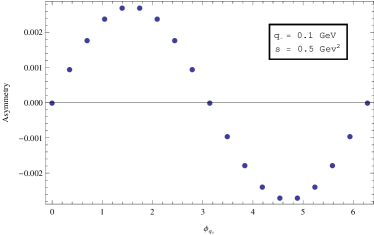
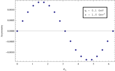
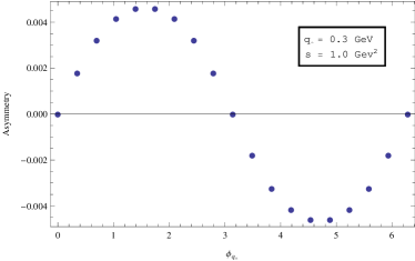
The figures below show the proton transverse target azimuthal SSA for various center of mass energies and momentum transfer. From the figures one notes that the asymmetry is positive and it increases with $q_{\perp}$ but decreases with the center of mass energy,as expected. On the other hand, the magnitudes of the amplitudes in the figures are consistent with the expected values for the transverse target SSA with unpolarized electrons beamย [2].

Refer to caption
Refer to caption
Refer to caption
Refer to caption
Figure 1: Proton transverse target azimuthal SSA for various center of mass energies and momentum transfers using GPD parametrization for the proton form factors

VI Conclusion

We study single spin azimuthal asymmetry in elastic electron-nucleon scattering for the case of transversely polarized nucleon with unpolarized electrons beam. The asymmetry in this case appears due to the interference between the $1\gamma$ and $2\gamma$ exchange amplitudes. To calculate the $(1)$ and $(2\gamma)$ Eikonal scattering amplitudes, we used the Coulomb/Eikonal phase associated with a transversely polarized nucleon, this phase is asymmetric in impact parameter space; consistent with the fact that the nucleon charge density (or the impact parameter dependent parton distribution function) is transversely distorted due to the transverse spin of the nucleon, which explains the existence of SSA in this case. Figure.1 shows the azimuthal target single spin asymmetry for different values of the center of mass energy and momentum transfer, as expected, the asymmetry increases with $q_{\perp}$ and decreases with the center of mass energy. The apmlitudes in the figures are consistent with the expected values of the transverse target SSA with unpolarized electrons beam. In the calculations, the transverse radius of the proton was taken from Ref.ย [20] and the GPD parametrization of the proton form factors from Ref.ย [21] while the integrals were evaluated numerically using the CUBA library for multidimensional numerical integrationย [22].

Appendix A Parametrization of Form Factors Using Generalized Parton Distributions

Generalized parton distribution (GPDs) can be considered as generalization of ordinary parton distributions. The formal definition of GPDs for transversely polarized nucleon but unpolarized quarks is given byย [23]

$\displaystyle\left<p^{\prime},S^{\prime}\vphantom{\hat{O}_{q}(x,\textbf{b}_{\perp})p,S}\right|\hat{O}_{q}(x,\textbf{b}_{\perp})\left|p,S\vphantom{p^{\prime},S^{\prime}\hat{O}_{q}(x,\textbf{b}_{\perp})}\right>\ =\ \frac{1}{2\bar{P}^{+}}\bar{u}(P^{\prime},S^{\prime})\left(\gamma^{+}\ H_{q}(x,\xi,t)\ +\ i\frac{\sigma^{+\nu}\Delta_{\nu}}{2M}E_{q}(x,\xi,t)\right)u(p,S)$ (27)

Where $\bar{P}^{\mu}=\frac{1}{2}(P^{\mu}+P^{\prime\mu})$ represents the average momentum of the target, $q^{\mu}=P^{\prime\mu}-P^{\mu}$ is the four momentum transfer, $t=q^{2}$ is the invariant momentum transfer and $\xi=-\frac{q^{+}}{2P^{+}}$ is the change in the longitudinal component of the target momentum and is called the skewness. The nucleons form factors can be decomposed as follows

Fip=euโ€‹Fiu+edโ€‹Fid+esโ€‹Fis,Fin=euโ€‹Fid+edโ€‹Fiu+esโ€‹Fisformulae-sequencesubscriptsuperscript๐น๐‘๐‘–subscript๐‘’๐‘ขsubscriptsuperscript๐น๐‘ข๐‘–subscript๐‘’๐‘‘subscriptsuperscript๐น๐‘‘๐‘–subscript๐‘’๐‘ subscriptsuperscript๐น๐‘ ๐‘–subscriptsuperscript๐น๐‘›๐‘–subscript๐‘’๐‘ขsubscriptsuperscript๐น๐‘‘๐‘–subscript๐‘’๐‘‘subscriptsuperscript๐น๐‘ข๐‘–subscript๐‘’๐‘ subscriptsuperscript๐น๐‘ ๐‘–\displaystyle F^{p}_{i}=e_{u}F^{u}_{i}+e_{d}F^{d}_{i}+e_{s}F^{s}_{i},\ \ \ \ F^{n}_{i}=e_{u}F^{d}_{i}+e_{d}F^{u}_{i}+e_{s}F^{s}_{i} (28)

Where $i=1,2$ and ย eu=23,ed=es=โˆ’13formulae-sequencesubscript๐‘’๐‘ข23subscript๐‘’๐‘‘subscript๐‘’๐‘ 13e_{u}=\frac{2}{3},\ e_{d}=e_{s}=\frac{-1}{3}. The Dirac and Pauli flavor form factors at zero skewness are give by the following sum rules

$\displaystyle F^{q}_{1}(t)=\int_{-1}^{1}dx\ H^{q}(x,\xi,t),\ \ \ \ F^{q}_{2}(t)=\int_{-1}^{1}dx\ E^{q}(x,\xi,t)$ (29)

The result of integration is independent of $\xi$. Also the integration region can be reduced to $0<x<1$ by introducing the non-forward parton densities

$\displaystyle\mathcal{H}^{q}(x,t)$ $\displaystyle=H^{q}(x,0,t)+H^{q}(-x,0,t),\ \ \ \ \mathcal{E}^{q}(x,t)=E^{q}(x,0,t)+E^{q}(-x,0,t)$ (30)

Where $q=u,d$ and $\mathcal{H}^{q}(x,t)$ reduces to the usual valence quark densities for $t\rightarrow 0$ for the up and down quarks. Thus, the form factors become

$\displaystyle F^{q}_{1}(t)=\int_{0}^{1}dx\ \mathcal{H}^{q}(x,t),\ \ \ \ F^{q}_{2}(t)=\int_{0}^{1}dx\ \mathcal{E}^{q}(x,t)$ (31)

The magnetic densities satisfies the following normalization conditions

$\displaystyle\kappa_{q}=\int_{0}^{1}dx\ \mathcal{E}^{q}(x),\ \ \ \kappa_{u}$ $\displaystyle=2\kappa_{p}+\kappa_{n}=+1.673,\ \ \ \kappa_{d}=\kappa_{p}+2\kappa_{n}=-2.033$ (32)
$\displaystyle F^{p}_{2}(t=0)$ $\displaystyle=1.793,\ \ \ \ F^{n}_{2}(t=0)=-1.913$

Followingย [21], the anzats for the Gโ€‹Pโ€‹Dโ€‹s๐บ๐‘ƒ๐ท๐‘ GPDs are The ansatz for the Gโ€‹Pโ€‹Dโ€‹s๐บ๐‘ƒ๐ท๐‘ GPDs isย [21]

$\displaystyle\mathcal{H}^{q}(x,t)$ $\displaystyle=q_{v}(x)x^{-\alpha^{\prime}(1-x)t},$ (33)
$\displaystyle\mathcal{E}^{q}(x,t)$ $\displaystyle=\frac{\kappa_{q}}{N_{q}}\left(1-x\right)^{\eta_{q}}q_{v}x^{-\alpha^{\prime}(1-x)t},$

The normalization constants $N_{q}$ satisfies

$$N_{q}=\int_{0}^{1}dx(1-x)^{\eta_{q}}q_{\nu}(x),$$ (34)

and the unpolarized parton distributions are parametrized as

$\displaystyle u_{\nu}(x)$ $\displaystyle=0.262x^{-0.69}(1-x)^{3.50}(1+3.83x^{0.5}+37.65x)$ (35)
$\displaystyle d_{\nu}(x)$ $\displaystyle=0.061x^{-0.65}(1-x)^{4.03}(1+49.05x^{0.5}+8.65x).$

The parameters used in this fit are $\alpha^{\prime}=1.105,\eta_{u}=1.713,\eta_{d}=0.566$. The following is a plot of $F_{1}$ and $F_{2}$ as a function of the momentum transfer.

References

  • [1] J.ย Arrington, P.G. Blunden, and W.ย Melnitchouk. Progress in Particle and Nuclear Physics, 66(4):782 โ€“ 833, 2011.
  • [2] Carlย E Carlson and Marc Vanderhaeghen. Two-photon physics in hadronic processes. arXiv preprint hep-ph/0701272, 2007.
  • [3] Andrei Afanasev, Mark Strikman, and Christian Weiss. Transverse target spin asymmetry in inclusive dis with two-photon exchange. Physical Review D, 77(1):014028, 2008.
  • [4] Marc Schlegel. Partonic description of the transverse target single-spin asymmetry in inclusive deep-inelastic scattering. Physical Review D, 87(3):034006, 2013.
  • [5] Dutta etย al. Measurements of target single-spin asymmetry in elastic ep scattering.
  • [6] F.E. Maas etย al. Phys.Rev.Lett., 94:082001, 2005.
  • [7] Androiฤ‡ etย al. Physical review letters, 107(2):022501, 2011.
  • [8] Armstrong etย al. Phys. Rev. Lett., 99:092301, Aug 2007.
  • [9] Matthias Burkardt. International Journal of Modern Physics A, 18(02):173โ€“207, 2003.
  • [10] Markus Diehl and Phย Hรคgler. The European Physical Journal C-Particles and Fields, 44(1):87โ€“101, 2005.
  • [11] Tareq Alhalholy and Matthias Burkardt. Impact parameter dependent potentials and average transverse momentum in inclusive dis. Phys. Rev. D, 93:125019, Jun 2016.
  • [12] Matthias Burkardt. Quark orbital angular momentum and final state interactions. In International Journal of Modern Physics: Conference Series, volumeย 25, page 1460029. World Scientific, 2014.
  • [13] A.ย Metz, D.ย Pitonyak, A.ย Schรคfer, M.ย Schlegel, W.ย Vogelsang, and J.ย Zhou. Phys. Rev. D, 86:094039, Nov 2012.
  • [14] A.ย De Rรบjula, J.M. Kaplan, and E.ย deย Rafael. Nuclear Physics B, 35(2):365 โ€“ 389, 1971.
  • [15] Andreiย V Afanasev, Stanleyย J Brodsky, Carlย E Carlson, Yu-Chun Chen, and Marc Vanderhaeghen. Physical Review D, 72(1):013008, 2005.
  • [16] Dmitry Borisyuk and Alexander Kobushkin. Phys. Rev. C, 72:035207, Sep 2005.
  • [17] Richardย C. Brower, Matthewย J. Strassler, and Chung-I Tan. Journal of High Energy Physics, 2009(03):050.
  • [18] Joseph Polchinski and Matthewย J. Strassler. Journal of High Energy Physics, 2003(05):012, 2003.
  • [19] Danielย N. Kabat. Validity of the Eikonal approximation. Comments Nucl. Part. Phys., 20(6):325โ€“335, 1992.
  • [20] Carlย E. Carlson and Marc Vanderhaeghen. Phys. Rev. Lett., 100:032004, Jan 2008.
  • [21] M.ย Guidal, M.ย V. Polyakov, A.ย V. Radyushkin, and M.ย Vanderhaeghen. Phys. Rev. D, 72:054013, Sep 2005.
  • [22] T.ย Hahn. Computer Physics Communications, 168(2):78 โ€“ 95, 2005.
  • [23] Geraldย A. Miller. Annual Review of Nuclear and Particle Science, 60(1):1โ€“25, 2010.