ExoMol molecular line lists - XVII The rotation-vibration spectrum of hot SO₃

Abstract

Sulphur trioxide (SO₃) is a trace species in the atmospheres of the Earth and Venus, as well as well as being an industrial product and an environmental pollutant. A variational line list for ³²S¹⁶O₃, named UYT2, is presented containing 21 billion vibration-rotation transitions. UYT2 can be used to model infrared spectra of SO₃ at wavelengths longwards of 2 $\mu$m ($\nu<5000$ cm^-1) for temperatures up to 800 K. Infrared absorption cross sections are also recorded at 300 and 500 C are used to validate the UYT2 line list. The intensities in UYT2 are scaled to match the measured cross sections. The line list is made available in electronic form as supplementary data to this article and at www.exomol.com.

1 Introduction

SO₃ known to exist naturally in the Earth’s atmosphere; its main source being volcanic emissions and hot springs (Michaud et al., 2005) but it also plays role in the formation of acid rain. The oxidisation of SO₂ to SO₃ in the atmosphere, followed by subsequent rapid reaction with water vapour results in the production of sulphuric acid (H₂SO₄) (Calvert et al., 1985) with many adverse environmental effects (Vahedpour et al., 2011; Kolb et al., 1994; Srivastava et al., 2004). So SO₃ is a natural product whose concentration in the atmosphere is significantly enhanced by human activity, particularly as a byproduct of industrialisation. SO₃ is observed in the products of combustion processes (Srivastava et al., 2004; Hieta & Merimaa, 2014) and selective catalytic reduction (SCR) units, where the presence of both is undesirable within flue gas chambers in large quantities, as well as other industrial exhausts (Rawlins et al., 2005; Fleig et al., 2012). The control of these outputs is therefore of great importance. The spectroscopic study of sulphur oxides can also provide insight into the history of the Earth’s atmosphere (Whitehill et al., 2013). All this means that observation of SO₃ spectra and hence concentrations provide a useful tool for understanding geological processes and controlling polution.

Sulphur oxide chemistry has been observed in a variety of astrophysical settings. Within the solar system, SO₃ is a constituent of the atmosphere of Venus (Craig et al., 1983; Zhang et al., 2010; Zhang et al., 2012). Although SO₃ has yet to be observed outside our solar system, it needs to be considered alongside other sulphur oxides namely, sulphur monoxide (SO) and SO₂, which are well-known in several astronomical environments (Na et al., 1990; Petuchowski & Bennett, 1992; Martin et al., 2003, 2005; Belyaev et al., 2012; Visscher et al., 2006; Belloche et al., 2013; Adande et al., 2013; Khayat et al., 2015). SO₃ chemistry has been considered in a number of enviroments including giant planets, brown dwarfs, and dwarf stars (Visscher et al., 2006). Unlike SO and SO₂, SO₃ is a symmetric species with no permanent dipole moment making it hard to detect in the interstellar medium. In practice, the identification of SO₃ in the infrared is hindered by the presence of interfering SO₂ where both species are found simultaneously; a number of their spectral features overlap, particularly the $\nu_{3}$ bands of both molecules in the 1300 - 1400 cm^-1 (7.4 $\mu$m) region. From this point of view SO₂ can also be seen as a spectral ‘weed’ with respect to the detection of SO₃. An understanding of the spectroscopic behaviour of both of these molecules within the same spectral window is therefore required to be able to correctly identify each species independently. In this context we note that a number of line lists are available for SO₂ isotopologues (Huang et al., 2014, 2016; Underwood et al., 2016); of particular relevence is the recent hot ExoAmes line list of Underwood et al. (2016).

The experimental spectroscopic studies of SO₃ have significant gaps, notably the absence of any measurement of absolute line intensities in the infrared. This may be attributed to its vigorous chemical reactivity which make measurements difficult. SO₃ is a symmetric planar molecule with equilibrium S-O bond lengths of 1.41732 Å and inter-bond angles of 120^∘ (Ortigoso et al., 1989), described by ${\mathcal{D}}_{3{\rm h}}$(M) symmetry. The $\nu_{1}$, $\nu_{2}$, $\nu_{3}$ and $\nu_{4}$ fundamental frequencies are attributed to the totally symmetric stretch at 1064.9 cm^-1(Barber et al., 2002), the symmetric bend at 497.5 cm^-1, and the asymmetric stretching and bending modes at 1391.5 and 530.1 cm^-1, respectively (Sharpe et al., 2003).

The infrared and coherent anti-stokes vibration-rotation spectra of a number of isotopologues of SO₃ have been extensively investigated in a series of papers by Maki and co-workers (Kaldor et al., 1973; Ortigoso et al., 1989; Chrysostom et al., 2001; Maki et al., 2001; Barber et al., 2002; Sharpe et al., 2003; Maki et al., 2004), reassessing and confirming fundamental constants and frequencies. 18 bands were analysed based on an empirical fitting to effective Hamiltonian models, yielding rovibrational constants and energy levels assigned by appropriate vibrational and rotational quantum numbers. Some temperature-dependent infrared cross sections are also available from laboratory studies (Grosch et al., 2013, 2015a), and we present new measurements in this work. Unlike all other measurements of SO₃ spectra, these cross sections are absolute. However, assigned spectra represented by line lists allow for the modelling of both absorption and emission spectra in different environments.

The “forbidden” rotational spectrum, for which centrifugal distortions can induce transitions, was investigated for the first time by Meyer et al. (1991) using microwave Fourier-transform spectroscopy. Assignments for 25 transitions were made, as well as the determination of a number of rotational constants, including the only direct measurement of the $C_{0}$ rotational constant. The work was analysed and extended theoretically (Underwood et al., 2014).

There have been a few studies on the ultraviolet spectrum of SO₃ by Fajans & Goodeve (1936), and Leroy et al. (1981), both between 220 and 270 nm where overlap with SO₂ is small. Burkholder & McKeen (1997) reported cross sections for the 195 to 330 nm range for the purposes of photolysis rate calculations of SO₃. All measurements were taken at room-temperature, and neither reported assignments for any of the bands, which exist as weak, diffuse vibrational band structures superimposed on a continuous background. As such, the rovibronic behaviour of SO₃ is much less well understood than for SO₂.

Prior to our studies, there was limited theoretical work on SO₃. Early work on anharmonic force constants (Dorney et al., 1973; Flament et al., 1992) for SO₃ led to first accurate, fully ab initio anharmonic quartic force field computed by Martin (1999). There have been no theoretical studies into the UV spectrum of SO₃. As for the experimental studies for SO₃, none of this work provided transition intensities. Our preliminary study for this project (Underwood et al., 2013), which produced the ab initio, room-temperature UYT line list, therefore provides the first absolute transition intensities for SO₃. These were used in the 2012 release of the HITRAN database (Rothman et al., 2013) to scale the relative experimental measurements allowing SO₃ to be included in the database for the first time. As discussed below, the present work suggest that these intensites may need to be reconsidered.

The present study on SO₃ was performed as part of the ExoMol project. ExoMol aims to provide comprehensive line lists of molecular transitions important for understanding hot atmospheres of exoplanets and other bodies (Tennyson & Yurchenko, 2012). Besides the ExoAmes SO₂ line list mentioned above, ExoMol has produced very extensive line lists for a number of polyatomic species including methane (CH₄) (Yurchenko & Tennyson, 2014), phosphine (PH₃) (Sousa-Silva et al., 2015), formaldehyde (H₂CO) (Al-Refaie et al., 2015b), hydrogen peroxide (HOOH) (Al-Refaie et al., 2015a) and nitric acid (HNO₃) (Pavlyuchko et al., 2015b). These line lists, all of which contain about 10 billion distinct vibration-rotation transitions, required the adoption of special computational procedures to make their calculation tractable. The UYT2 SO₃ line list presented here is the largest computed so far with 21 billion lines; as SO₃ is a system comprising four heavy atoms this meant considering rotation states up to $J=130$ as part of these calculations. These calculations therefore required further enhancement of our computational methods which are described below. The lack of measured SO₃ spectra at temperatures above 300 K on an absolute scale is clearly a problem for validating our calculations. Here we present infrared absorption cross sections for SO₃ measured at a range of temperatures up to 500 C.

The next section describes our theoretical procedures; our experiments are described in section 3. Section 4 presents the UYT2 line list. Section 5 compares the UYT2 line list with our measurements with a particular emphasis on intensity comparisons. The final section gives details on how to access the line list and our conclusions.

2 Theoretical method

To compute a variational line list requires three components (Lodi & Tennyson, 2010): a suitable potential energy surface (PES), dipole moment surfaces (DMS), and a nuclear motion program. Variational nuclear motion programs, which use basis functions to provide direct solutions of the rotation-vibration Schrödinger equation for a given PES, means that interactions between the levels associated with different vibrational states and the associated intensity stealing between these bands are automatically included in the calculation. In particular, the use of exact kinetic energy operators means that how well these effects are reproduced depends strongly on the PES used; the reader is refered to a recent study by Zak et al. (2016) for a discussion of this.

Here the nuclear motion calculations are performed with the flexible, polyatomic vibration-rotation nuclear motion program TROVE (Yurchenko et al., 2007). The ab initio DMS surface was adopted unaltered from our previous calculations (Underwood et al., 2013) (UYT); below we describe refinement of the PES. Both the ab initio PES and DMS were computed at the coupled-clusters level of theory (CCSD(T)-F12b) level of theory with appropriate triple-$\zeta$ basis sets, aug-cc-pVTZ-F12 and aug-cc-pV(T+d)Z-F12 for O and S, respectively.

The label F12 in the theoretical model denotes the use of explicitly correlated functions which are designed to accelarate basis set convergence. The F12b varient is an efficient F12 implementation due to Adler et al. (2007). Use of CCSD(T)-F12b methods have been shown to give improved vibrational frequencies compared to standard CCSD(T) calculations (Martin & Kesharwani, 2014) but their use for intensity calculations remains relatively untested. We return to this issue below.

2.1 Refining the Potential Energy Surface

The refinement of the ab initio  PES involved performing a least-squares fit to empirical rovibrational energies or observed transition frequencies. The procedure follows that described elsewhere (Yurchenko et al., 2011; Yachmenev et al., 2011; Sousa-Silva et al., 2013; Yurchenko & Tennyson, 2014) and is based on adding a correction, $\Delta V$, to the ab initio UYT PES, which is represented by an expansion

$$\Delta V = \sum_{ijklmn}\,\Delta f_{ijklmn}\xi_{1}^{i}\xi_{2}^{j}\xi_{3}^{k}\xi_{4}^{l}\xi_{5}^{m}\xi_{6}^{n}\,\$$ (1)

in terms of the same internal coordinates as UYT Underwood et al. (2013):

$$\xi_{k} = 1-\exp(-a(r_{k}-r_{\rm e}))\hbox{,}\;\;k=1,2,3,$$ (2)

$$\xi_{4} = \frac{1}{\sqrt{6}}\left(2\alpha_{23}-\alpha_{13}-\alpha_{12}\right)\hbox{,}$$ (3)

$$\xi_{5} = \frac{1}{\sqrt{2}}\left(\alpha_{13}-\alpha_{12}\right)\hbox{,}$$ (4)

$$\xi_{6} = \sin\rho_{e}-\sin{\bar{\rho}}\hbox{,}$$ (5)

where

$$\sin{\bar{\rho}}\,=\,\frac{2}{\sqrt{3}}\,\sin[(\alpha_{23}+\alpha_{13}+\alpha_{12})/6]$$ (6)

$\sin\rho_{e}$ is the equilibrium value of $\sin\bar{\rho}$, $a$ is a molecular parameter, and $\Delta f_{ijk\ldots}$ are expansion coefficients. Here $r_{i}$ is a bond length and $\alpha_{ij}$ is an interbond bond angle. Further details of this functional form and symmetry relations between $\Delta f_{ijk\ldots}$ can be found elsewhere (Yurchenko et al., 2005b; Underwood et al., 2013).

The refined potential coefficients $\Delta f_{ijk\ldots}$ were determined using a least squares fitting algorithm which uses the derivatives of energies with respect to $\Delta f_{ijk\ldots}$ computed via the Hellmann-Feynman theorem (Feynman, 1939). The process starts by setting all $\Delta f_{ijk\ldots}=0$. The resulting refined PES is only an ‘effective’ one since it depends on any approximation in the nuclear motion calculations; it is therefore dependent on the levels of kinetic energy (KE) and PES expansion, and basis set used (see below). As a result of this, improving the nuclear motion calculation may lead to worse agreement with the observations.

The experimental data for the energies is taken from the extensive high resolution infrared studies of Maki and co-workers (Kaldor et al., 1973; Ortigoso et al., 1989; Chrysostom et al., 2001; Maki et al., 2001; Barber et al., 2002; Sharpe et al., 2003; Maki et al., 2004). The majority of these studies provide upper and lower energy states labelled by their vibrational normal mode and rotational ($J$, $K$) quantum numbers, which were validated using effective Hamiltonians. However, the bands studied by Maki et al. (2004) label transitions by rotational and vibrational quantum numbers, but do not list upper and lower energy levels. Combination differences were used to obtain energies for these bands using the experimental line positions reported by the accompanying publications; these are highlighted in Table 1. In matching experimental and computed energies, a number of experimentally derived energies were not included in the fit; these correspond to transitions excluded by Maki et al. from their Hamiltonian fits. A total of 119 energy levels for $J\leq$ 5 were chosen from this set based on their reliability at reproducing the observed transitions, with the condition that they are physically accessible states with $A^{\prime}$ or $A^{\prime\prime}$ symmetry; any published values of experimentally-derived purely vibrational terms (i.e. band centres) that are inaccessible were not included. Table 3 lists all the $J$ = 5 levels used in the refinement process, comparing with their final computed counterparts.

Table 1: Comparison of RMS differences for the ab initio (UYT) and refined (UYT2) PES for observed vibrational band centres of SO₃. Values for band centres are the experimental ones of (Maki et al., 2001). All values are in cm^-1. Note: UYT does not cover transition frequencies above 4000 cm^-1.

Band	Band Centre	UYT	UYT2
2$\nu_{2}$ - $\nu_{2}$	497.45	0.73	0.09
$\nu_{2}$ - $\nu_{0}$	497.57	0.77	0.05
$\nu_{2}$ + $\nu_{4}$ - $\nu_{4}$	497.81	0.82	0.03
2$\nu_{4}^{(l_{4}=0)}$ - $\nu_{4}$	529.72	1.33	0.30
$\nu_{4}$ - $\nu_{0}$	530.09	1.41	0.09
$\nu_{2}$ + $\nu_{4}$ - $\nu_{2}$	530.33	0.22	0.08
2$\nu_{4}^{(l_{4}=2)}$ - $\nu_{4}$	530.36	1.54	0.37
$\nu_{1}$ - $\nu_{4}$	534.83	0.47	0.20
$\nu_{3}$ - $\nu_{0}$	1391.52	4.06	0.09
2$\nu_{2}$ + $\nu_{4}$ - $\nu_{0}$	1525.61	0.19	0.08
§$\nu_{2}$ + 2$\nu_{4}^{(l_{4}=0)}$ - $\nu_{0}$	1557.88	2.39	1.17
§$\nu_{2}$ + 2$\nu_{4}^{(l_{4}=2)}$ - $\nu_{0}$	1558.52	2.12	0.64
§$\nu_{1}$ + $\nu_{2}$ - $\nu_{0}$	1560.60	1.14	1.28
§3$\nu_{4}^{l_{4}=1}$ - $\nu_{0}$	1589.81	6.73	4.00
§$\nu_{1}$ + $\nu_{4}^{(l_{4}=1)}$ - $\nu_{0}$	1593.69	3.32	3.57
⋆§($\nu_{3}$ + $\nu_{4}$)(L=2) - $\nu_{0}$	1917.68	5.34	0.65
2$\nu_{3}^{(l_{3}=2)}-\nu_{0}$	2777.87	7.53	0.20
§3$\nu_{3}^{(l_{3}=1)}$ - $\nu_{0}$	4136.39	–	0.08

^⋆The value $L$ is given by $L$ = $|l_{3}+l_{4}|$, see Maki et al. (2004).

^§These bands are refined using energy levels obtained from the data by (Maki et al., 2001, 2004) via combination differences.

Table 2: Comparisons of vibrational ($J$ = 0) terms for SO₃, between experimental values (Maki et al., 2001), and the ab initio (UYT) and refined (UYT2) PES. All values are given in cm^-1.

	Obs.	UYT	UYT2
$\nu_{2}$	497.57	498.48	497.56
$\nu_{4}$	530.09	528.59	530.09
2$\nu_{2}$	995.02	995.35	993.67
$\nu_{2}$ + $\nu_{4}^{(l_{4}=1)}$	1027.90	1027.35	1027.33
2$\nu_{4}^{(l_{4}=0)}$	1059.81	1056.50	1059.48
2$\nu_{4}^{(l_{4}=2)}$	1060.45	1057.38	1060.45
$\nu_{1}$	1064.92	1065.75	1066.49
$\nu_{3}$	1391.52	1387.45	1391.51
3$\nu_{2}$	1492.35	1490.76	1488.47
2$\nu_{2}$ + $\nu_{4}^{(l_{4}=1)}$	1525.61	1524.48	1524.20
$\nu_{2}$ + 2$\nu_{4}^{(l_{4}=0)}$	1557.88	1555.59	1557.50
$\nu_{2}$ + 2$\nu_{4}^{(l_{4}=2)}$	1558.52	1556.45	1558.46
$\nu_{1}$ + $\nu_{2}$	1560.60	1565.33	1565.07
3$\nu_{4}^{(l_{4}=1)}$	1589.81	1586.46	1588.97
3$\nu_{4}^{(l_{4}=3)}$	1591.10	1586.43	1591.06
$\nu_{1}$ + $\nu_{4}^{(l_{4}=1)}$	1593.69	1593.36	1595.92
$\nu_{2}$ + $\nu_{3}^{(l_{3}=1)}$	1884.57	1881.53	1884.29
⋆($\nu_{3}$ + $\nu_{4}$)(L=2)	1917.68	1912.24	1917.68
⋆($\nu_{3}$ + $\nu_{4}$)(L=0)	1918.23	1914.56	1919.63
2$\nu_{3}^{(l_{3}=0)}$	2766.40	2759.12	2766.38
2$\nu_{3}^{(l_{3}=2)}$	2777.87	2770.29	2777.86
3$\nu_{3}^{(l_{3}=1)}$	4136.39	4126.78	4136.33

^⋆The value $L$ is given by $L$ = $|l_{3}+l_{4}|$, see Maki et al. (2004).

Table 3: Observed (Maki et al., 2001) minus Calculated residuals for the $J$ = 5 energy levels used in the refinement procedure. All values are in cm^-1. The corresponding values for $J\leq$ 5 are given in Underwood (2016).

State	$K$	Obs.	UYT2	Obs. - Calc.
$\nu_{0}$	3	8.885	8.886	-0.001
$\nu_{2}$	3	506.367	506.360	0.008
	0	507.900	507.893	0.007
	5	535.323	535.312	0.011
$\nu_{4}^{(l_{4}=1)}$	4	538.471	538.490	-0.020
	2	539.561	539.560	0.001
	1	540.677	540.685	-0.008
2$\nu_{2}$	3	1002.357	1002.411	-0.054
$\nu_{2}$ + $\nu_{4}^{(l_{4}=1)}$	5	1033.102	1033.058	0.044
	4	1036.241	1036.226	0.016
	2	1037.252	1037.219	0.033
	1	1038.243	1038.220	0.023
	5	1068.278	1068.303	-0.025
2$\nu_{4}^{(l_{4}=0)}$	3	1068.461	1068.456	0.005
2$\nu_{4}^{(l_{4}=2)}$	2	1071.024	1071.031	-0.007
	5	1398.427	1398.437	-0.010
$\nu_{3}^{(l_{3}=1)}$	2	1401.580	1401.581	-0.001
	1	1401.599	1401.591	0.009
	5	1529.365	1529.362	0.003
2$\nu_{2}$ + $\nu_{4}^{(l_{4}=1)}$	4	1532.498	1532.520	-0.022
	2	1533.442	1533.448	-0.006
$\nu_{1}$ + $\nu_{2}$	3	1573.870	1573.856	0.014
	0	1575.400	1575.387	0.013
3$\nu_{4}^{(l_{4}=1)}$	4	1597.408	1597.410	-0.002
$\nu_{1}$ + $\nu_{4}^{(l_{4}=1)}$	5	1601.162	1601.150	0.012
	4	1604.308	1604.322	-0.014
	2	1605.430	1605.426	0.004
	1	1606.574	1606.577	-0.002
	5	1923.797	1923.808	-0.011
⋆($\nu_{3}$ + $\nu_{4}$)(L=2)	4	1925.310	1925.318	-0.008
	0	1927.488	1927.422	0.066
	1	1927.982	1927.988	-0.006
	5	2782.262	2782.227	0.035
2$\nu_{3}^{(l_{3}=2)}$	4	2786.812	2786.837	-0.025
	2	2786.901	2786.888	0.014
	1	2788.419	2788.425	-0.006
3$\nu_{3}^{(l_{3}=1)}$	5	4143.316	4143.246	0.070
	2	4146.379	4146.329	0.050

^⋆The value $L$ is given by $L$ = $|l_{3}+l_{4}|$, see Maki et al. (2004).

Table 1 shows the effect of the final potential refinement on the bands used in the refining procedure. The root mean square (RMS) differences are calculated by matching all experimental lines for each band with calculated values via their quantum number assignments for all $J\leq$ 5 available.

The RMS differences calculated are slightly increased when including higher $J>5$ term values comparing to the residuals in Table 3 for a few bands as a result of the refinement, namely the $\nu_{1}$ + $\nu_{2}$ and $\nu_{1}$ + $\nu_{4}^{(l_{4}=1)}$ bands. The experimental energy levels used to refine these two bands were obtained using combination differences. However, for some rotationally excited levels within these bands, the quantum number labelling of the experimental transitions appears dubious: in particular there are a number of transition whose labels are duplicated. These transitions were not included in the RMS difference calculations but there must be some doubt about the validity of the quantum number assignments of the other transitions in these bands. This may well explain the increased the RMS difference.

Table 2 compares all published vibrational ($J$ = 0) term values with those calculated with TROVE before and after refinement. There are some discrepancies introduced by the refinement procedure and in some cases deteriorations from the pre-refined values (e.g 2$\nu_{2}$). The quality of the refinement can be assessed from Table 1, with the exception of 3$\nu_{2}$, for which there is no experimental band data available beyond the quoted vibrational term value (Maki et al., 2004).

Our refined PES is given as Supplementary Information to this article.

2.2 Calculation using TROVE

In specifying a calculation using TROVE, it is necessary to fix a number of parameters. In particular both the KE and PES are expanded as a Taylor series about the equilibrium geometry (Yurchenko et al., 2007). For UYT the expansions were truncated at 4^th and 8^th orders respectively. Here the KE expansion order was increased to 6^th in order to allow better convergence. For the detailed description of the basis set see Underwood et al. (2013). Here it suffices to define the maximal polyad number $P_{\rm max}$ used in TROVE to control the size of the basis set. The polyad number in case of SO₃ in terms of the normal mode quantum numbers is given by

$$P=2(n_{1}+n_{3})+n_{2}+n_{4},$$ (7)

where $n_{1},n_{2},n_{3}$ and $n_{4}$ are the normal mode quanta associated with the $\nu_{1},\nu_{2},\nu_{3}$ and $\nu_{4}$ vibrational modes. For the UYT2 calculations the value of $P_{\rm max}$ was set initially to $24$ for the 1D primitive basis functions to form a product-type basis set, which was then contracted to $P_{\rm max}=18$ after a set of prediagonalizations of reduced Hamiltonian matrices and symmetrized. The value of $P_{\rm max}$ used for UYT was 12. This increase was necessary to allow both better convergence of the increased number of energies which is needed for high temperature spectra. Only energies lying up to 10 000 cm^-1 above the ground state were considered as part of this study.

The high symmetry of ³²S¹⁶O₃, and the associated nuclear spin statistics, means that it is only necessary to consider transitions between $A_{1}^{\prime}$ and $A_{1}^{\prime\prime}$ symmetries of the ${\mathcal{D}}_{3{\rm h}}$ point group used for the calculations. The final UYT2 line list consists of all allowed transitions between 0 $<\nu\leq$ 5000 cm^-1, satisfying the conditions $E^{\prime}\leq 9000$ cm^-1, $E^{\prime\prime}\leq 4000$ cm^-1 and $J\leq$ 130. These parameters are designed to give a complete spectrum up to 5000 cm^-1 ($\lambda>2$ $\mu$m) for temperatures up to about 800 K. Generating a complete line list with these parameters is computationally demanding and therefore requires special measures to be taken.

In terms of memory, diagonalisation of the Hamiltonian matrices is the most computationally expensive part of the line list calculation. For each $J$, a matrix is built (Yurchenko et al., 2007; Yurchenko et al., 2009) and then stored in the memory for diagonalisation, using an appropriate eigensolver routine. TROVE uses a symmetry adapted basis set representation and allows splitting of each $J$ Hamiltonian matrix further into the six symmetry blocks ($A_{1}^{\prime}$, $A_{2}^{\prime}$, $E^{\prime}$, $A_{1}^{\prime\prime}$, $A_{2}^{\prime\prime}$, and $E^{\prime\prime}$) which are dealt with separately. Since only the $A_{1}^{\prime}$ and $A_{1}^{\prime\prime}$ symmetry species are allowed by the nuclear statistics of ³²S¹⁶O₃, only these symmetry blocks are diagonalized.

Memory requirements scale with the square of the dimension of the Hamiltonian matrix, $N^{\rm Ham}_{J}$. This is given roughly by $N^{\rm Ham}_{J}=N_{J=0}\times(2J+1)$, where $N_{J=0}$ is the dimension of the purely vibrational matrix. For UYT2, the combined dimension $N_{J=0}$ of both $A_{1}^{\prime}$ and $A_{1}^{\prime\prime}$ symmetries is 2692; for comparison, the UYT line list calculations used $N_{J=0}$ = 679. The size of the largest matrix considered in the room-temperature calculations (for $J$ = 85) is $N^{\rm Ham}_{85}=111~{}296$, which is already surpassed by $J$ = 21 for UYT2 for which the value of $N^{\rm Ham}_{85}=454~{}488$. It became quickly apparent that the diagonalisation techniques previously employed to determine the UYT wavefunctions would be impractical for UYT2.

Nuclear motion calculations were performed using both the Darwin and COSMOS HPC facilities in Cambridge, UK. Each of the computing nodes on the Darwin cluster provide 16 CPUs across two 2.60 GHz 8-core Intel Sandy Bridge E5-2670 processors, and a maximum of 64 Gb of RAM. The advantage of moving eigenfunction calculations to the Darwin cluster are that an entire node can be dedicated to one calculation, spread across the 16 CPUs. Since multiple nodes can be accessed by a single user at any time, multiple computations were carried out simultaneously.

Diagonalisation of matrices with $J\leq$ 32 was possible using the LAPACK DSYEV eigensolver (Anderson et al., 1999), optimised for OpenMP parallelisation across multiple (16) CPUs. For 32 $<J\leq$ 90 a distributed memory approach was used with an MPI-optimised version of the eigensolver, PDSYEVD, which allowed diagonalisations across multiple Darwin/COSMOS nodes in order to make use of their collective memory. In order to diagonalise the matrix within the 36 hour wall clock limit, it was necessary to perform this method in three steps. First, for a given $J$ and symmetry species $\Gamma$, the Hamiltonian matrix was constructed and saved to disk. Secondly, the matrix was then read and diagonalised using PDSYEVD across the number of nodes required to store of the matrix in their shared memory. This produces a set of eigenvectors which were read in again to convert into the TROVE eigenfunction format.

For $J>$ 90 yet another approach was developed for use on the COSMOS shared memory machine. This method employed the PLASMA DSYTRDX routine (Kurzak et al., 2013) and, unlike the above procedure, constructed, diagonalised and stored wavefunctions to disk in a single process by extending both the standard wallclock time and memory limits. For $J$ = 130 ($\Gamma$ = $A_{1}^{\prime}$) a total of 52 hours of real time was taken to construct and diagonalize the Hamiltonian matrix across 416 CPUs, and utilising 3140 Gb of RAM.

While matrix diagonalisation dominates the memory requirements of the calculation, computing the line strengths, $S(f\leftarrow i)$, is the major user of computer time. In principle line strengths for all transitions obeying the rigorous electric dipole selection rules, $\Delta J=J^{\prime}-J^{\prime\prime}=0,\pm 1\ (J^{\prime\prime}+J^{\prime}\geq 1)$ and $A_{1}^{\prime}\leftrightarrow A_{1}^{\prime\prime}$, were computed. In practice this was modified to reduce the computational demands. Firstly, calculations of the line strength only take into consideration the basis functions of the final state wavefunction whose coefficients are greater than 10^-14. In addition to this a threshold value for the Einstein A coefficient of 10^-74 s^-1 dictates which transitions are kept. However, the number of line strength calculations to be performed still remains very large and even with parallelisation across multiple Darwin CPUs, performing the calculations proved to be both computationally expensive and difficult.

To help expedite these computations, an adapted version of TROVE was used which is optimised for performing calculations on graphical processing units (GPUs). The use of this implementation, known as GAIN (GPU Accelarated INtensities) (Al-Refaie et al., 2016), allowed for the computation of transition strengths for the more computationally demanding parts of the calculations. These calculations were performed on the Emerald GPU cluster, based in Southampton. In general, the calculation of transition strengths across multiple GPUs was much faster than the Darwin CPUs. For example, there are a total of 349 481 979 transitions for $J^{\prime\prime}$ = 35, which took a total of 17 338 CPU hours to compute on the Darwin nodes, compared to 2053 GPU hours on the Emerald nodes for 346 620 894 transitions for the larger $J^{\prime\prime}$ = 59 case. These GPU calculations were carried out for those $J\leftrightarrow\ J+1$ pairs containing a large number of states, while the Darwin CPUs were reserved for the less computationally demanding sections.

21 billion transitions were calculated for UYT2, which is two orders of magnitude larger than UYT. Overall performing the computations needed for the UYT2 line list took us over 2 years.

3 Experiments

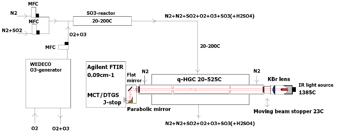
Figure 1: Set up used for SO₂/SO₃/O₃ infrared absorption measurements.

SO₃ absorbance measurements at temperatures up to 500 C were performed using a quartz high-temperature gas flow cell (q-HGC). The cell has been described in details by Grosch et al. (2013) and has recently been used for measurements with NH₃ (Barton et al., 2015), S-containing gases (Grosch et al., 2015a) and some PAH compounds (Grosch et al., 2015b).

Because SO₃ is an extremely reactive gas and normally contains traces of SO₂ if ordered from a gas supplier, it was decided to produce SO₃ directly in the set up. It is known that SO₂ can react with O₃ and form SO₃:

$${\rm SO}_{2}+{\rm O}_{3}\rightarrow{\rm SO}_{3}+{\rm O}_{2}.$$ (8)

The rate constant for the reaction (8) is temperature dependent: higher temperatures favour SO₃ formation. However at higher temperatures O₃ starts to decompose into O₂ and O:

$${\rm O}_{3}(+{\rm M})\rightarrow{\rm O}_{2}+{\rm O}(+{\rm M})$$ (9)

Some O and O₂ can contribute further in SO₃ formation and “re-cycle” O₃:

$${\rm SO}_{2}+{\rm O}(+{\rm M}) \rightarrow {\rm SO}_{3}(+M)$$

$${\rm O}+{\rm O}_{2}(+{\rm M}) \rightarrow {\rm O}_{3}(+{\rm M})$$

$${\rm O}+{\rm O}(+{\rm M}) \rightarrow {\rm O}_{2}(+{\rm M})$$ (10)

If any water traces are present in the system, SO₃ will rapidly be converted into sulfuric acid (H₂SO₄):

$${\rm SO}_{3}+{\rm H}_{2}{\rm O}(+{\rm M})\rightarrow{\rm H}_{2}{\rm SO}_{4}(+{\rm M}),$$ (11)

which is then followed by further surface-promoted reaction:

$${\rm H}_{2}{\rm SO}_{4}+{\rm surface}\rightarrow{\rm products}.$$ (12)

Other possible SO₃ removal channels are:

$${\rm SO}_{3}(+{\rm M}) \rightarrow {\rm SO}_{2}+{\rm O}(+{\rm M})$$

$${\rm SO}_{3}+{\rm surface} \rightarrow {\rm products}.$$ (13)

These reactions are very prominent in a clean set up with “active” surfaces.

In the presence of O₂, a reversible reaction (which is also temperature-dependent) takes place:

$$2{\rm SO}_{2}+{\rm O}_{2}(+{\rm M})\rightarrow 2{\rm SO}_{3}(+{\rm M}).$$ (14)

However SO₃ formation through reaction (14) takes place at temperatures higher than 500 C. The set-up is shown in Fig. 1. It can be divided into two parts: a SO₃ generation part and a part for optical measurements.

The optical part of the set up includes a high-resolution FTIR spectrometer (Agilent 660 with a linearized broad-band MCT detector), the q-HGC and a light-source (Hawkeye, IR-Si217, 1385C) with a KBr plano-convex lens. The light source is placed in the focus of the KBr lens. The FTIR and sections between the FTIR/q-GHC and q-HGC/IR light source have been purged by CO₂/H₂O-free air obtained from a purge generator.

The O₃-generation part consists of a set of high-end mass-flow controllers (MFC’s), O₃-generator and a unit called SO₃-reactor. MFC’s (Bronkhorst) have been used to keep constant gas flows and mix gas flows of N₂, N₂+SO₂ and O₂+O₃ in desirable ratios. An O₃-generator (WEDECO GSO 30, water cooled, rated capacity at full load 100 g hour^-1 of O₃ with use of O₂) was used to produce O₃ from O₂. Because of the high O₂ flow rate required for stable operation of the O₃-generator, only a part of the O₂+O₃ flow was used in the measurements. The ozone generator was operated at about 30% (225 W) of the full load. SO₃-reactor was a 50 cm heated quartz tube (20 – 200 C) with inner diameter of 50 mm. N₂+SO₂ was mixed in the SO₃-reactor with O₂+O₃ from the ozone-generator at 170 – 190 C. The gas residence time in the O₃-reactor was about 60 s at 1 l_n min^-1 (normal litres per minute) flow rate which was enough to convert about 50% of SO₂ into SO₃ and at the same time mostly decompose O₃. The SO₃-reactor was connected through a heated Teflon-line (inner diameter 4 mm, $T=$ 20 – 200 C) to the inlet of the q-HGC. The gas residence time in the Teflon-line was about 0.8 s (at 1 ln/min) and some further (minor) conversion of SO₂ to SO₃ took also place.

Bottles with premixed gas mixture, N₂ + SO₂ (5000ppm) (Strandmöllen) and N₂/O₂ (99.998%) (AGA) have been used for reference and SO₂/SO₃ absorbance measurements. The main flow in the q-HGC was balanced with the two buffer flows of N₂ from q-HGC’s buffer parts. Most of SO₂/SO₃ absorbance measurements have performed at 0.25-0.5 cm^-1 nominal spectral resolutions and around atmospheric pressure in the q-HGC. Few measurements have been performed at 0.09 cm^-1 spectra resolution. The measurements were performed in following steps:

1. N₂ + O₂ in q-HGC, reference spectra, ozone generator “off”;

2. N₂ + O₂ + SO₂ (2500 ppm) in q-HGC, absorption spectra, ozone generator “off”;

3. N₂ + O₂ + SO₂ + SO₃ + O₃ in q-HGC, absorption spectra, ozone generator “on”, initial SO₂ concentration 2500 ppm;

4. N₂ + O₂ + O₃, in q-HGC, ozone generator “on” in order to measure O₃ traces in the q-HGC (addition step used only for some measurements).

O₃ has several absorption bands in 400-6000 cm^-1, which do not interfere with SO₂/SO₃ absorption bands. At each step two measurements were made: with a light source (emission from the cell and light source) and without a light source (emission from the cell). Experimental absorption spectra SO₂/SO₃ were reconstructed in the way described in section 3.1 of Barton et al. (2015). Spectra of SO₂ measured in step 2 have been normalized and subtracted from the composite SO₂+SO₃ spectra obtained in step 3 in order to get the zero absorption signal in vicinity of the SO₂ bands as one can see in Fig. 2. It was further assumed that all SO₂ was consumed to produce SO₃ (i.e. no SO₃ losses channels). Note various log10-absorption scales on these figures. The extra (weak) broad feature in the region 1200-1285 cm^-1 is caused by the O₃ production in the O₃-generator.

Figure 3 gives a comparison of our newly measured cross sections in the 7.4 $\mu$m region with those available from the PNNL database for SO₂ (upper) and SO₃ (lower).

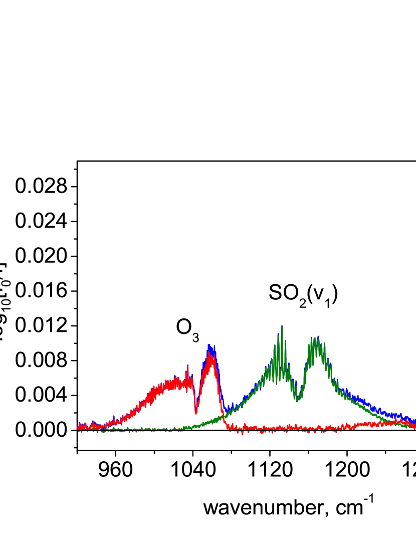
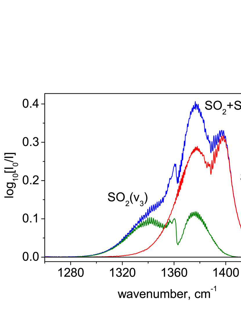
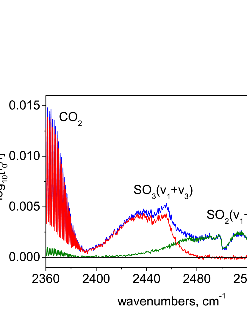
Figure 2: Composite SO₂+SO₃+O₃ absorption spectrum at 300 C (blue) together with (normalized) SO₂ spectrum (olive) and the result of subtraction of SO₂ spectrum from the composite one (red): The vicinity of the $\nu_{1}$ (upper), $\nu_{3}$ (middle) and $\nu_{1}+\nu_{3}$(lower) bands of SO₂.

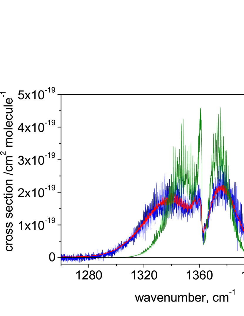
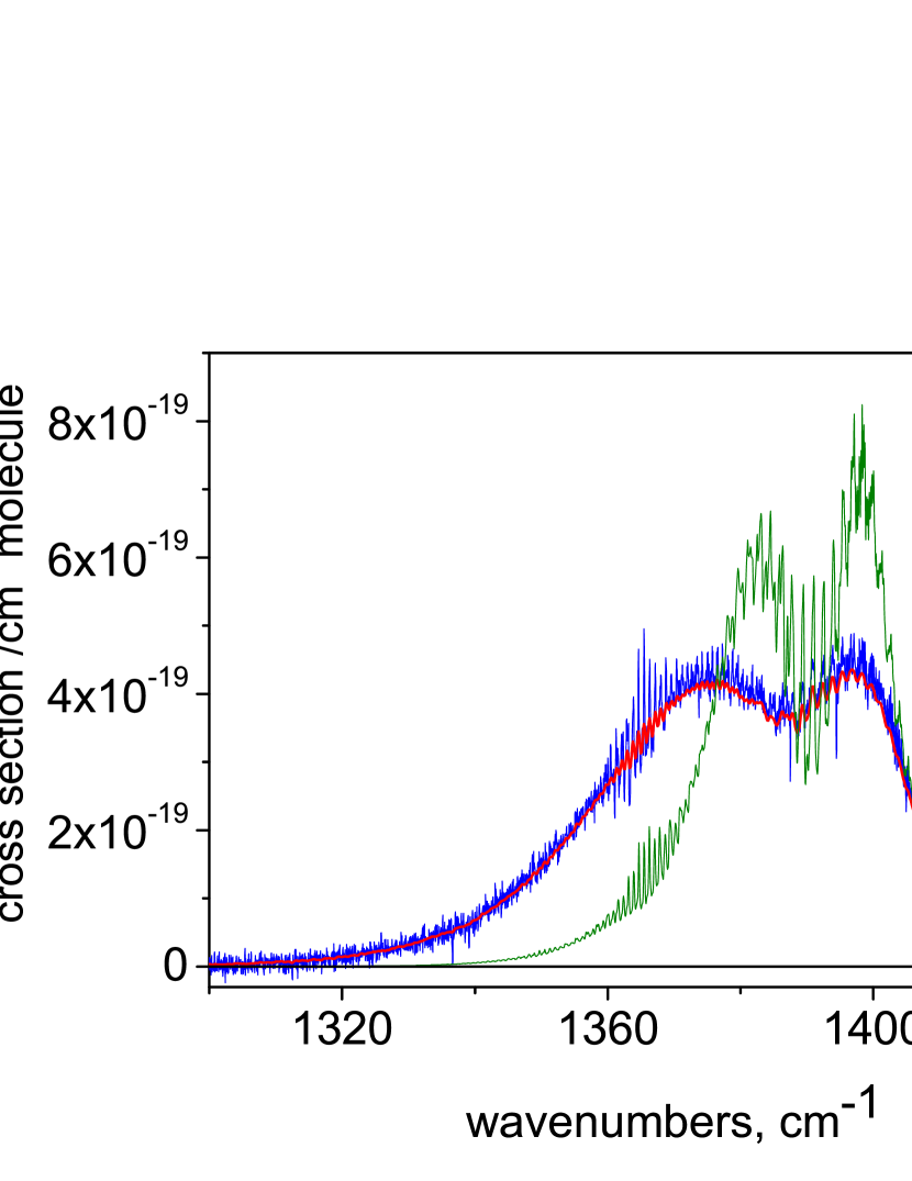
Figure 3: SO₂ (upper) and SO₃ (lower) absorption cross sections at 400 C: 0.09 cm^-1 (blue, boxcar), 0.5 cm^-1 (red, triangular). Cross section from PNNL database at 25 C (olive, 0.112 cm^-1, boxcar) are shown for comparison.

4 Overview of the UYT2 Line List

The UYT2 line list is presented in the ExoMol format (Tennyson et al., 2013, 2016) with main data contained in a states and a set of transtions files. Tables 4 and 6 give portions of these files. The complete files can be obtained via ftp://cdsarc.u-strasbg.fr/pub/cats/J/MNRAS/xxx/yy, or http://cdsarc.u-strasbg.fr/viz-bin/qcat?J/MNRAS//xxx/yy, as well as the exomol website, www.exomol.com.

Table 4: Extract from the UTY2 state file for SO₃; quantum numbers are specified in Table 5. The full table is available from http://cdsarc.u-strasbg.fr/cgi-bin/VizieR?-source=J/MNRAS/xxx/yy.

$n$	$\tilde{E}$	$g$	$J$	$\Gamma_{\rm Total}$	$K$	$\Gamma_{\rm Rot}$	$v_{1}$	$v_{2}$	$v_{3}$	$v_{4}$	$v_{5}$	$v_{6}$	$n_{1}$	$n_{2}$	$n_{3}$	$L_{3}$	$n_{4}$	$L_{4}$	$\Gamma_{\rm Vib}$
1	0.0000	1	0	1	0	1	0	0	0	0	0	0	0	0	0	0	0	0	1
2	993.6780	1	0	1	0	1	0	0	0	0	0	2	0	2	0	0	0	0	1
3	1059.4770	1	0	1	0	1	0	0	0	0	2	0	0	0	0	0	2	0	1
4	1066.4970	1	0	1	0	1	1	0	0	0	0	0	1	0	0	0	0	0	1
5	1591.0349	1	0	1	0	1	0	0	0	0	3	0	0	0	0	0	3	1	1
6	1919.6346	1	0	1	0	1	1	0	0	0	1	0	0	0	1	1	1	1	1
7	1981.9944	1	0	1	0	1	0	0	0	0	0	4	0	4	0	0	0	0	1
8	2054.0505	1	0	1	0	1	0	0	0	0	2	2	0	2	0	0	2	0	1
9	2061.9334	1	0	1	0	1	1	0	0	0	0	2	1	2	0	0	0	0	1
10	2117.4659	1	0	1	0	1	0	0	0	0	4	0	0	0	0	0	4	0	1
11	2124.4973	1	0	1	0	1	1	0	0	0	2	0	1	0	0	0	2	0	1
12	2129.3331	1	0	1	0	1	0	1	1	0	0	0	2	0	0	0	0	0	1
13	2444.1614	1	0	1	0	1	1	0	0	0	2	0	0	0	1	1	2	2	1
14	2586.0493	1	0	1	0	1	0	0	0	0	3	2	0	2	0	0	3	1	1
15	2648.2382	1	0	1	0	1	0	0	0	0	5	0	0	0	0	0	5	1	1
16	2655.7551	1	0	1	0	1	1	0	0	0	3	0	1	0	0	0	3	1	1
17	2766.3812	1	0	1	0	1	0	2	0	0	0	0	0	0	2	0	0	0	1
18	2904.3481	1	0	1	0	1	1	0	0	0	1	2	0	2	1	1	1	1	1

Table 5: Quantum numbers used in labelling energy states.

Quantum Number	Description
$n$	Counting index
$\tilde{E}$	Energy value (cm-1)
$g$	Total degeneracy of the state
$J$	Angular momentum quantum number
$\Gamma_{\rm Total}$	Total symmetry in ${\mathcal{D}}_{3{\rm h}}$(M): 1 = $A_{1}^{\prime}$, 4 = $A_{1}^{\prime\prime}$
$K$	Projection of $J$ on to the $z$-axis
$\Gamma_{\rm Rot}$	Rotational symmetry in ${\mathcal{D}}_{3{\rm h}}$(M): 1 = $A_{1}^{\prime}$, 2 = $A_{2}^{\prime}$, 3 = $E^{\prime}$ , 4 = $A_{1}^{\prime\prime}$, 5 = $A_{2}^{\prime\prime}$, 6 = $E^{\prime\prime}$
$v_{i},i=1-6$	Local mode vibrational quantum numbers
$n_{1}$, $n_{2}$, $n_{3}$, $n_{4}$	Normal mode vibrational quantum numbers
$L_{3}$, $L_{4}$	$L$ projections of the vibrational angular momenta
$\Gamma_{\rm Vib}$	Vibrational symmetry in ${\mathcal{D}}_{3{\rm h}}$(M): 1 = $A_{1}^{\prime}$, 2 = $A_{2}^{\prime}$, 3 = $E^{\prime}$ , 4 = $A_{1}^{\prime\prime}$, 5 = $A_{2}^{\prime\prime}$, 6 = $E^{\prime\prime}$

Table 6: Extract from the UTY2 transitions file for SO₃. The full table is available from http://cdsarc.u-strasbg.fr/cgi-bin/VizieR?-source=J/MNRAS/xxx/yy.

$f$	$i$	A
237007	249581	1.1253e-17
158430	148459	2.8358e-17
549592	568676	1.3725e-16
120670	112002	1.4546e-16
2080392	2117071	9.0696e-18
289088	302965	1.4938e-16
393104	377035	1.5764e-16
43637	49289	2.1375e-16
587986	607961	2.0370e-16
587868	647986	4.2068e-18
2007259	2043487	5.2490e-18
627725	648113	3.0673e-16

$f$: Upper state counting number; $i$: Lower state counting number; $A_{fi}$: Einstein-A coefficient in s^-1.

The energy levels listed in the states file are labelled with the quantum numbers summarised in Table 5 and are based on those recommended by Down et al. (2013) for ammonia with the simplification that one does not need to consider inversion. Only quantum numbers $J$, $g_{\rm Total}$, $\Gamma_{\rm Total}$ and the counting index, $n$ are rigorously defined. The remaining quantum numbers represent the largest contribution from rotational and vibrational components of the wavefunction expansion associated with a given state. TROVE provides local mode quantum numbers associated with the basis set construction scheme used (Underwood et al., 2013). The normal mode vibrational quantum numbers, $n_{1}$, $n_{2}$, $n_{3}$ and $n_{4}$, and or their angular momentum projections $L_{3}$ = $|l_{3}|$ and $L_{4}$ = $|l_{4}|$ were obtained from the local mode quantum numbers via the correlation rules

$$n_{1}+n_{3} = v_{1}+v_{2}+v_{3},$$ (15)

$$n_{2}+n_{4} = v_{4}+v_{5}+v_{6},$$ (16)

and

$$l_{3} = -v_{3},-v_{3}+2,...,v_{3}-2,v_{3},$$ (17)

$$l_{4} = -v_{4},-v_{4}+2,...,v_{4}-2,v_{4},$$ (18)

where $v_{1}$, $v_{2}$ and $v_{3}$ are three stretching, $v_{4}$ and $v_{5}$ are two deformational (asymmetric) bending and $v_{6}$ is inversion local mode (TROVE) quantum numbers. The mapping between these quantum numbers for a particular level also required knowledge of the energy value and symmetry, since multiple levels may be labelled with the same local mode quantum numbers. In these ambiguous cases, the symmetric modes quantum numbers $n_{1}$ and $n_{2}$ were chosen for the lower energies, and $n_{3}$ and $n_{4}$ with the higher, and that $L_{3}$ and $L_{4}$ increase proportionally with the energies, and are multiples of 3 in the case of $A_{1}$ or $A_{2}$ symmetries, or otherwise for the $E$-type symmetry. This mapping is performed by hand at the $J$ = 0 stage of the calculation, and then propagated to $J>$ 0.

The Einstein-$A$ coefficient for a particular transition from the initial state $i$ to the final state $f$ is given by:

$$A_{if}=\frac{8\pi^{4}\tilde{\nu}_{if}^{3}}{3h}(2J_{i}+1)\sum_{A=X,Y,Z}|\langle\Psi^{f}|\bar{\mu}_{A}|\Psi^{i}\rangle|^{2},$$ (19)

where $h$ is Planck’s constant, $\tilde{\nu}_{if}$ is the wavenumber of the line, ($hc\,\tilde{\nu}_{if}=E_{f}-E_{i}$), $J_{i}$ is the rotational quantum number for the initial state, $\Psi^{f}$ and $\Psi^{i}$ represent the TROVE eigenfunctions of the final and initial states respectively, $\bar{\mu}_{A}$ is the electronically averaged component of the dipole moment along the space-fixed axis $A=X,Y,Z$ (see also Yurchenko et al. (2005a)).

In order to calculate the absorption intensity for a given temperature $T$ only five quantities are required (all provided by UYT2), the transition wavenumber $\tilde{\nu}_{if}$, the Einstein coefficient $A_{if}$, the lower (initial) state energy term value $\tilde{E}_{i}$, the total degeneracy of the upper (final) state $g_{f}=g_{\rm ns}J_{f}(J_{f}+1)$, and the partition function $Q(T)$, as given by

$$I(f\leftarrow i)=\frac{A_{if}}{8\pi c}\frac{g_{f}}{Q\;\tilde{\nu}_{if}^{2}}\exp\left(-\frac{c_{2}\tilde{E}_{i}}{T}\right)\left[1-\exp\left(\frac{-c_{2}\tilde{\nu}_{if}}{T}\right)\right],$$ (20)

where $c_{2}$ is the second radiation constant, $g_{\rm ns}$ is the nuclear spin statistical weight factor ($g_{\rm ns}$ = 1 for ³²S¹⁶O₃), $c$ is the speed of light. The partition function $Q$ is given by:

$$Q=\sum_{i}g_{i}\exp\left({\frac{-c_{2}\tilde{E}_{i}}{T}}\right).$$ (21)

For a line list to be suitable for modelling spectra at a certain temperature it is necessary for the partition function, $Q$, to be converged at this temperature. This is equivalent to stating that all energy levels that are significantly populated at the given temperature, $T$, must be considered. This convergence gives a metric upon which line list completeness can be gauged (Neale et al., 1996).

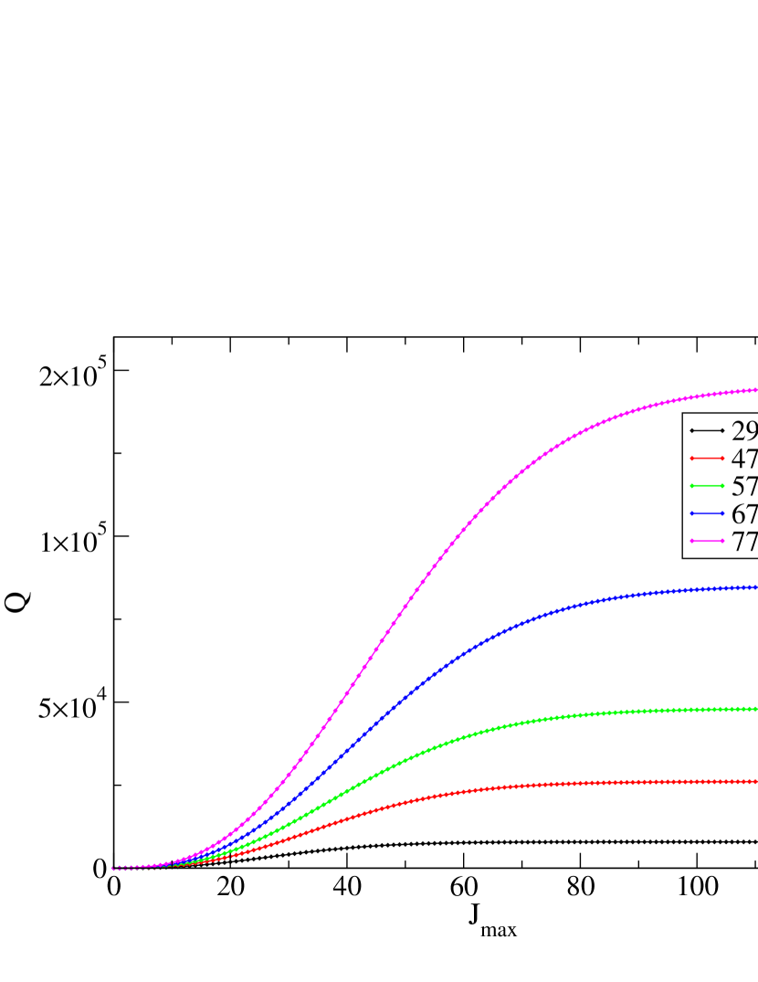
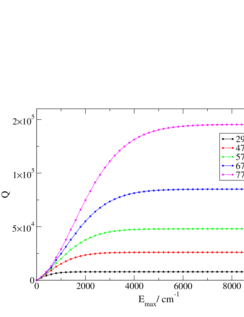
Figure 4: Convergence of partition function at different temperatures as a function of $J_{\rm max}$ (upper) and $E_{\rm max}$ (lower). The partition function increases monotonically with temperature.

Figure 4 shows convergence of the partition function with $J_{\rm max}$ for different temperatures, $T$. Upon inspection, the value of $Q$ is adequately converged at $J$ = 130 for $T\leq 800$ K. Table 7 shows the final values of $Q$ obtained for selected temperature alongside their estimated degree of convergence. As can be seen, the value of $Q$ = 7908.906 at $T$ = 298.15 K calculated from UYT2 is in agreement with the value of $Q$ = 7908.266 obtained from UYT.

Table 7: Values of the partition function, $Q$, for different temperatures, $T$. The degree of convergence is specified by $Q_{J_{130}}-Q_{J_{129}}/Q_{J_{130}}\times$ 100.

T (K)	Q	Degree of Convergence (%)
298.15	7908.906	6.27 $\times\ 10^{-6}$
473.15	26065.642	8.50 $\times\ 10^{-4}$
573.15	48007.866	3.62 $\times\ 10^{-3}$
673.15	85016.645	9.99 $\times\ 10^{-3}$
773.15	145389.574	2.12 $\times\ 10^{-2}$
1000	437353.233

For the purposes of determining completeness of the line list, it is more appropriate to view the convergence of $Q$ as a function of an energy cut-off, $E_{\rm max}$. This is also shown in Figure 4, from where it is clear from that imposing this limit will have a non-negligible effect on a spectral simulation at $T$ = 773.15 K, in particular; since the partition function is not fully converged at $E_{\rm max}$ = 4000 cm^-1 it is expected that levels with energies above this value will also be populated to some extent. This would be manifest as certain lines being missing from the spectrum, where transitions from levels contributing with some significance to the partition function are not included. Similarly, the truncation of calculations at $J$ = 130 means that a number of potentially contributing energy levels are omitted from the partition sum at $T$ = 773.15 K; at $J$ = 130 the lowest energy lies around 4000 cm^-1. This means that the high-$T$ partition function obtained will be slightly lower than the fully converged value.

It is possible to quantify the completeness of the line list by assuming that the value of $Q$ at $J$ = 130 is close enough to the ‘true’ value of the partition function at the given temperature. Figure 5 shows the ratio of the value of the partition function at the 4000 cm^-1 cut-off and the assumed total partition function, $Q_{\rm Total}$. At $T$ = 773.15 K, the line list is roughly 90% complete. In reality, this is an upper limit due to the fact that there is a slight underestimation of $Q_{\rm Total}$ at this temperature. However, the contribution from the missing energies with $J>$ 130, which all lie above 4000 cm^-1, can be estimated to be small enough not to affect $Q_{\rm Total}$ by more than 1% below $T=800$ K.

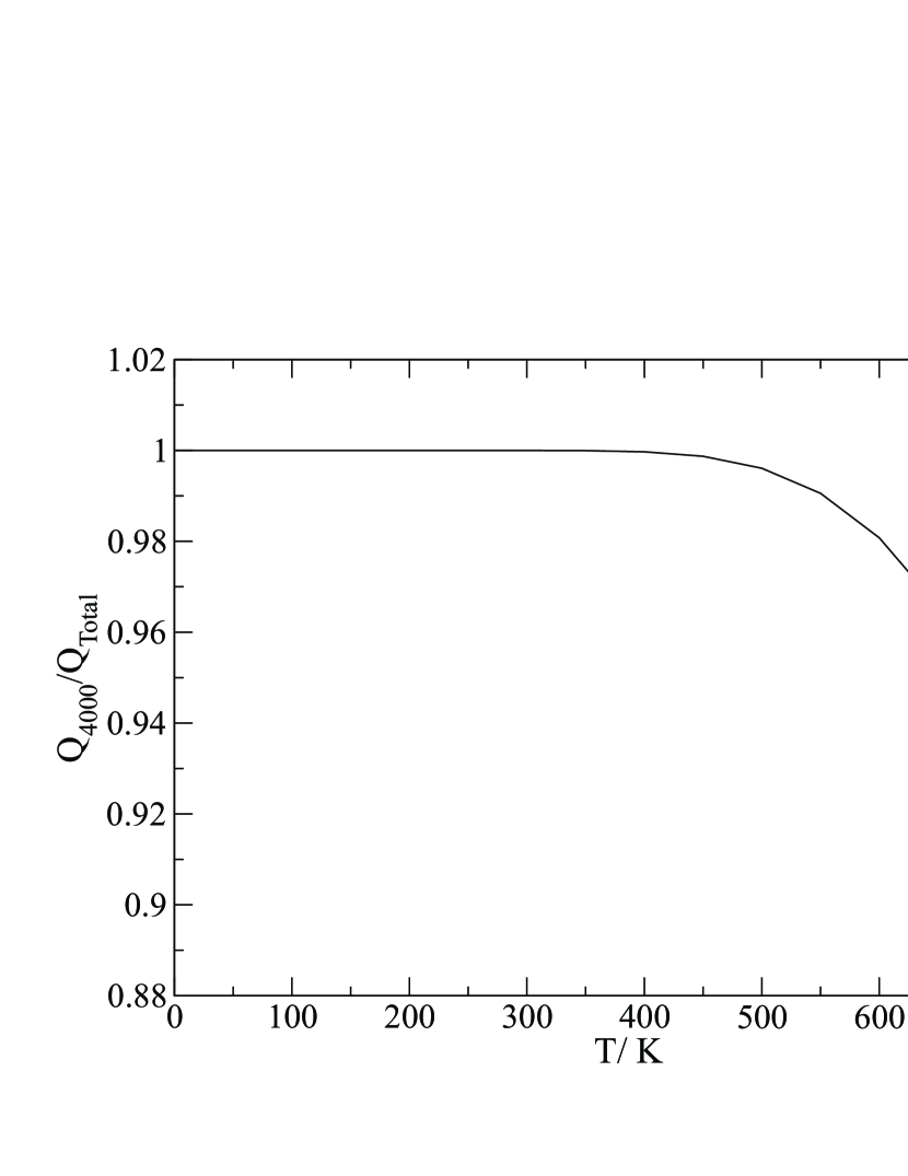
Figure 5: Ratios of $Q_{4000}$ to the assumed converged values $Q_{\rm Total}$ as a function of temperature.

5 Intensity Comparisons

UYT (Underwood et al., 2013) made extensive intensity comparisons with the available, room temperature, high resolution, infrared spectra due to Maki et al.; in general finding good agreement. However, these experimental spectra are not absolute so the comparison is only for relative intensities. A comparison of the intensities predicted by the UYT and UYT2 line lists are summarised in Table 8. This comparison essentially shows that UYT2 reproduces the band intensities of UYT, showing that adjusting PES does not significantly alter the computed intensities, as has occasionally been found to happen (Al-Refaie et al., 2015b).

Table 8: Comparison of calculated band intensities in cm/molecule$\times 10^{-18}$. Units are given in 10^-18 cm molecule^-1.

Band	Band Intensity
	UYT	UYT2
2$\nu_{2}$ - $\nu_{2}$	0.66	0.62
$\nu_{2}$	3.71	3.39
$\nu_{2}$ + $\nu_{4}$ -$\nu_{4}$	0.58	0.54
$\nu_{4}$	5.95	5.37
2$\nu_{4}^{(l_{4}=0)}$ - $\nu_{4}$	0.41	0.44
$\nu_{2}$ + $\nu_{4}$ - $\nu_{2}$	0.53	0.49
2$\nu_{4}^{(l_{4}=2)}$ - $\nu_{4}$	0.87	1.17
$\nu_{1}$ - $\nu_{4}$	0.10	0.22
$\nu_{3}$	44.44	43.21
2$\nu_{3}^{(l_{3}=2)}-\nu_{0}$	0.12	0.11

Since the comparison with the data of Maki et al. is only able to provide a measure of the quality of relative intensities within a particular band, an absolute intensity comparison is highly desirable. The new measured temperature-dependent DTU SO₃ cross section data plus the room-temperature cross sections in the PNNL (Pacific Northwest National Laboratory) database (Sharpe et al., 2004) provide this possibility. For both data sets there are discernible spectral features across four separate regions and it should be possible to make a semiquantitative analysis by comparing integrated intensities across a given spectral window. To make this comparison cross sections were generated from UYT2 using the ExoCross tool (Hill et al., 2013; Tennyson et al., 2016).

Figure 6 shows comparisons between recorded cross sections from PNNL at 298.15 K (25^∘C) and resolution 0.112 cm^-1, compared with simulated cross sections using the full UYT2 line list, based on a Gaussian profile of HWHM = 0.1 cm^-1. Figure 7 gives a similar comparison for the $\nu_{1}+\nu_{3}$ and 2$\nu_{3}$ bands.

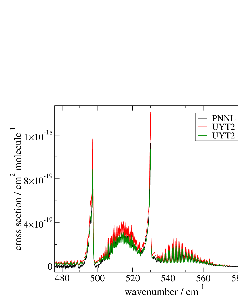
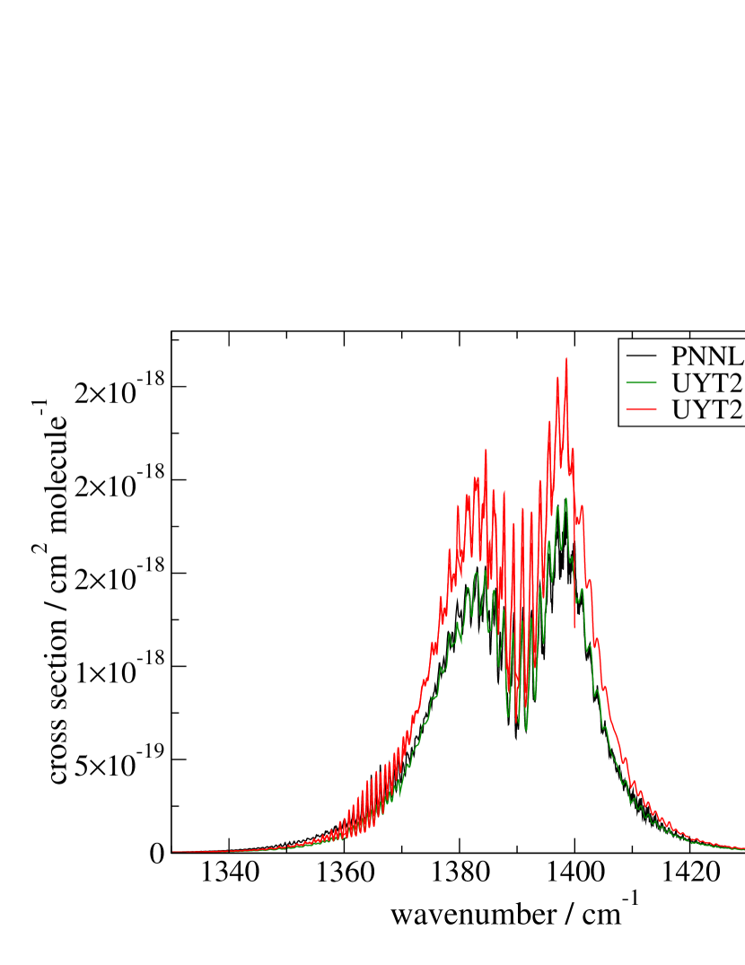
Figure 6: Comparisons of the $\nu_{2}$ and $\nu_{4}$ bands (upper) and the $\nu_{3}$ band (lower) for PNNL (Sharpe et al., 2004) and simulated cross sections at $T$ = 298.15 K.

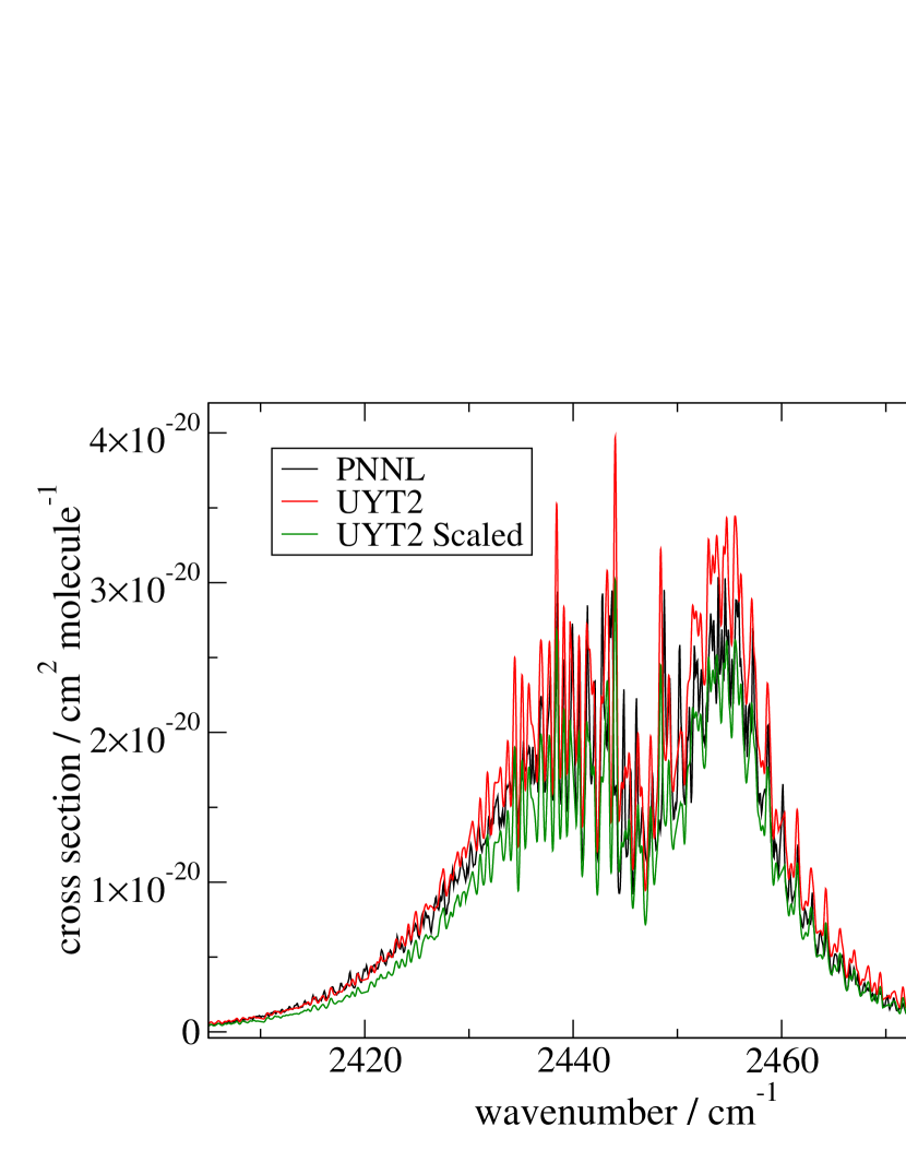
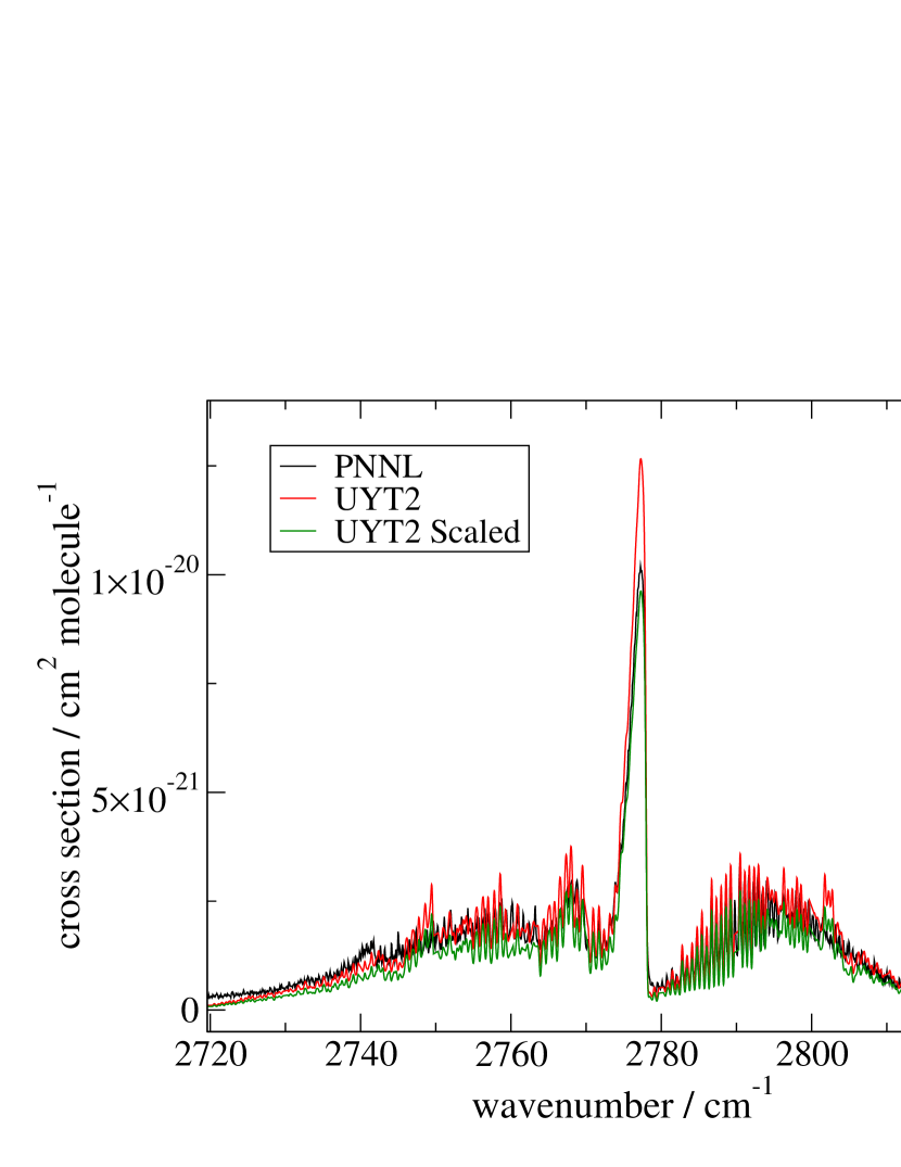
Figure 7: Comparisons of the $\nu_{1}+\nu_{3}$ bands (upper) and the 2$\nu_{3}$ band (lower) for PNNL (Sharpe et al., 2004) and simulated cross sections at $T$ = 298.15 K.

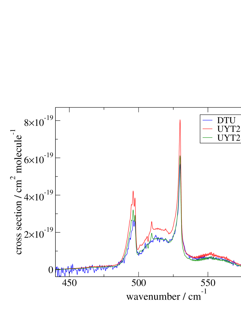
Figure 8: Comparisons of the $\nu_{2}$ and $\nu_{4}$ bands (upper) and the $\nu_{3}$ band (lower) for experimentally obtained (this work) and simulated cross sections at $T$ = 573.15 K.

Figure 8 shows a comparison of the the $\nu_{2}$ and $\nu_{4}$ complex and the $\nu_{3}$ band between cross sections recorded for SO₃ at 573.15 K (300^∘C) and those simulated using the UYT2 line list, based on a Gaussian profile of HWHM = 0.25 cm^-1, this value is the one which gives the best representation of the experimental spectra. In practice, the integrated intensity across the spectral region is largely independent of the HWHM value used. Figure 9 shows the same comparison for the $\nu_{1}+\nu_{3}$ band, which appears in a noisier region of the spectrum, and is also disturbed by a strong, foreign absorption feature resulting from the presence of CO₂. There is no data at $T$ = 573.15 K for the 2$\nu_{3}$ band due to noise contamination in the associated spectral region. Measurements of SO₃ were also made for 773.15 K (500^∘C), however it has not been possible to generate accurate experimental cross section values due to difficulties in estimating the concentration within the gas flow cell. The integrated absorption cross sections reconstructed from the experimental data at 500^∘C are larger values than those at lower temperatures ($<$ 500^∘C) suggesting non-conservation of the integrals over the various SO₃ bands. This might be explained by other, probably hetero-phase processes, which give rise to different SO₃ concentrations than one would expect from the assumption made that all SO₂ consumed in the reaction (8) gives raise of SO₃.

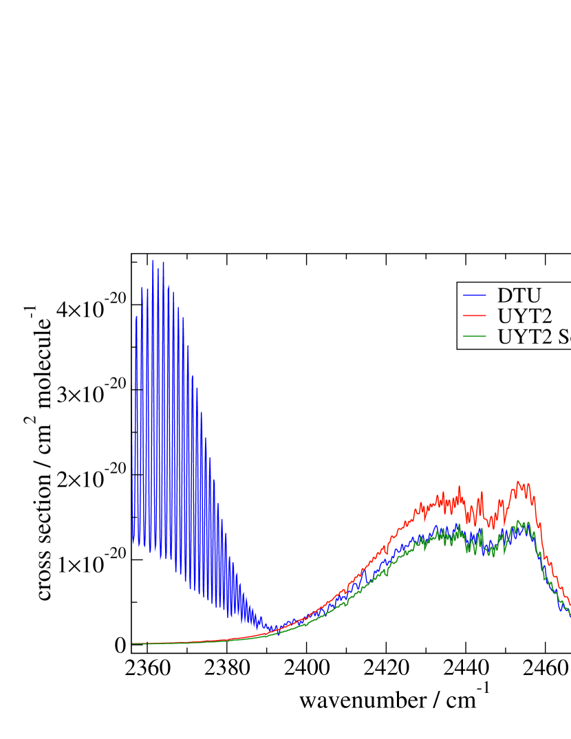
Figure 9: Comparisons of the $\nu_{1}$ + $\nu_{3}$ bands for experimental (this work) and simulated cross sections at $T$ = 573.15 K.

The comparisons reveals that although band positions and features are fairly well represented, there is a clear tendency for the UYT2 data to overestimate the line intensities for both temperatures considered. In our experience of computing ab initio intensities it is common for whole bands to have intensities which are over/underestimated by a constant factor (Lodi et al., 2008). However, we have not previously encountered a situation where the intensities of all the bands are shifted by a similar amount. There are a number of possibilities that could explain such a discrepancy. Firstly, it is possible that the experimental cross sections may be underestimated due to an overestimate of the SO₃ abundance; the calculation of cross sections requires the knowledge of the species concentration within the length of the absorption cell (Barton et al., 2015). However, the fact that measurements at room-temperature performed at DTU corroborate the PNNL data, and that similar discrepancies are observed for both data sets suggests that this is not the case. In this context it is worth noting that a similar comparison for SO₂ yields good agreement between measure and ab initio absolute cross sections (Underwood et al., 2016).

A second possible source of disagreement could be convergence issues with the partition function. Since the calculated intensities given by Eq. (20) depend on the scaling factor $Q(T)$ the incorrect computation of this value at the given temperature will lead to inaccurate values of absolute intensity. The difference in integrated cross section intensities observed suggest that, if the calculated value of $Q(T)$ is incorrect, then it is smaller than the ‘true’ value, since the theoretical cross sections are more intense than the experimentally observed values. This scenario can also be ruled out, due to two reasons. First, the agreement between $Q(T)$ for both UYT and UYT2 is very good at $T$ = 298.15 K, where they are both adequately converged; the increased basis set size underlaying the UYT2 calculations would undoubtedly account for any missing rovibrational energies in UYT. Secondly, and perhaps more interestingly, the analysis of several bands across different temperatures shows the cross section discrepancies to be almost independent of the value of $T$ (see below). This would not be expected if $Q(T)$ were the source of the disagreement, since partition sums can be expected to converge differently as a function of temperature.

This heavily implies that the problem lies with the DMS defects are by no means unknown (Al-Refaie et al., 2015b; Pavlyuchko et al., 2015a; Azzam et al., 2015), despite previous experience of obtaining accurate ab initio dipole surfaces (Lodi et al., 2011; Polyansky et al., 2015). We therefore undertook a small series of new ab initio calculations to see if we could identify the source of this problem. These calculations were all performed with MOLPRO (Werner et al., 2012) at the CCSD(T) level using finite differences. First we compared the original CCSD(T)-F12b with triple-$\zeta$ basis sets (aug-cc-pVTZ-F12 on O and aug-cc-pV(T+d)Z-F12 on S) results with calculations performed at the more traditional CCSD(T) with the same basis sets. The results were very similar suggesting that use of F12b what neither the cause of the problem nor was it providing improved convergence. Second we repeated the CCSD(T) using a larger quadrupole-zeta basis set (aug-cc-pVQZ-F12 on O and aug-cc-pV(Q+d)Z-F12 on S). The dipoles computed at this level proved to be somewhat smaller suggesting that the UYT DMS suffers from a lack of convergence in the one-particle basis set. Further work on this problem is left to future work. Here we adopt the more pragmatic approach of scaling our computed intensities.

It is not easy to make a rigorous analysis based on cross section data available for SO₃, as it is not immediately obvious what the contributions are from individual lines. In addition to this, both data sets contain varying degrees of noise within certain spectral regions, with the region around the $\nu_{3}$ band generally providing the best signal. Pavlyuchko et al. (2015a) performed a fit of their DMS based on experimental intensity data for nitric acid, to better improve simulated intensities. The lack of absolute intensity measurements for SO₃, coupled with the expensive computational demands of the line list calculation make this particularly difficult to perform here. Nevertheless, the best approach has been to compare integrated band intensities across fixed spectral windows to obtain scaling parameters for the each band. Table 9 summarises the ratios of integrated intensities between simulated and recorded cross sections for some available bands. These were obtained by explicit numerical integration over the wavenumber range of the corresponding regions.

Table 9: Intensities integrated over the corresponding band region for observed and calculated (UYT2) cross sections as a function of temperature, $T$. Intensity units are given in 10^-18 cm molecule^-1.

$T$ (K)	Band	Integrated Intensity		Obs./UYT2
		Obs.	UYT2
298.15	$\nu_{2}\ \&\ \nu_{4}$	9.95	13.13	0.76
	$\nu_{3}$	46.78	60.38	0.77
	$\nu_{1}+\nu_{3}$	0.71	0.82	0.87
	2$\nu_{3}$	0.15	0.16	0.97
573.15	$\nu_{2}\ \&\ \nu_{4}$	10.26	13.53	0.76
	$\nu_{3}$	46.79	59.62	0.78
	$\nu_{1}+\nu_{3}$	0.69	0.87	0.79

For most bands there appears to be a fairly consistent shift in intensity values across different temperatures, however the overtone bands for $T$ = 298.15 K suggest otherwise. The differences are quite subtle; for example, while the 2$\nu_{3}$ band has almost perfect agreement in integrated intensity across the band, the central $Q$-branch peak is not well represented by the UYT2 cross sections. On the other hand, the DTU data at 573.15 K for the $\nu_{1}+\nu_{3}$ band exhibits the same general shift as the $\nu_{2}$, $\nu_{3}$ and $\nu_{4}$ bands when care is taken exclude the intensity due to contamination in the integration, but the same is not true at room-temperature. The PNNL room-temperature cross sections are presented as a composite spectrum created from 8 individual absorbance spectra taken at various different pressures using both a mid-band MCT and wide-band-MCT detector, and uncertainties in intensity are listed as 10%. The measurements at DTU were performed several times and over different years, when the cell was used for other measurements. The data however are well-reproducible. Up to 400^∘C agreement in integrated absorption cross sections between DTU and PNNL is from 0 % to 13 % for strongest bands that is the same order as PNNL’s uncertainties in bands intensity. If the scaling factors for the two overtone bands at room-temperature are ignored, then the remaining factors may be averaged and applied to all simulated cross sections. This gives an average scaling factor of 0.76. The assumption made here is that the apparent better agreement in the room-temperature intensities for the $\nu_{1}+\nu_{3}$ and 2$\nu_{3}$ are ‘accidental’, while the wide, coverage-consistent high-temperature cross sections provide a more accurate description of the differences. Previous experience suggests that an ab initio DMS is more likely to overestimate rather than underestimate intensities (Schwenke & Partridge, 2000; Tennyson, 2014; Azzam et al., 2015). Without extra experimental data for more bands at different temperatures it is difficult to ascertain whether the intensity overestimates seen here are consistent for all bands or vary with different vibrational transitions.

Figures 6 and 7 show the various bands at room-temperature, with computed cross sections multiplied by the averaged scaling factor. Figures 8 and 9 show the same for $T$ = 573.15 K, which improve the simulated cross sections, and demonstrate the implied temperature independent nature of the discrepancy. As can be seen in Figure 7, using the averaged scaling factor (obtained from excluding the individual $\nu_{1}+\nu_{3}$ and 2$\nu_{3}$ Obs./UYT2 ratios) improves the reproduction of the central band peak, though the $P$-branch does show some intensity differences. This appears to be common for multiple bands and is possibly due to our neglecting of pressure broadening when generating the cross sections.

Figure 10 shows the cross sections calculated over the entire spectral range of 0 $<\nu\leq$ 5000 cm^-1, using a Gaussian profile of HWHM = 0.25 cm^-1, for a number of different temperatures. All simulated cross sections have been multiplied by the average scaling factor of 0.76. As can be seen, the region beyond 4500 cm^-1 shows some anomalies for higher temperatures, for this reason it is recommended that this region be treated with caution.

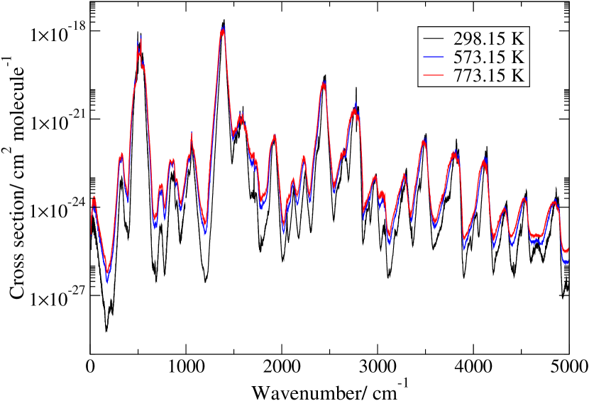
Figure 10: Overview of the simulated cross sections using UYT2, at $T$ = 298.15, 473.15 and 773.15 K, with a Gaussian profile of HWHM = 0.25 cm^-1. The dips in the cross sections are progressively smoothed out with increasing temperature. For higher temperatures, the region beyond 4500 cm^-1 appears anomalous, and should be treated with caution.

6 Conclusion

The UYT2 line list contains 21 billion transitions, and a total of 18 million energy levels below 10 000cm^-1. This provides an improvement upon the initial room-temperature line list, UYT, in terms of both line positions and temperature coverage. Table 1 provides a measure of the improvement introduced by the PES refinement present in the UYT2 line list. The total RMS deviation for the bands included in the potential adjustment is 1.35 cm^-1, compared to 3.23 cm^-1 for the unrefined PES of UYT. The majority of simulated line positions across these bands is improved by an order of magnitude.

It is difficult to ascertain the overall quality of the ab initio DMS used in the production of line intensities. However comparing with newly available cross section data at two different temperatures heavily suggests that the DMS used in the calculation of intensities is slightly overestimated, causing an apparently constant shift in all intensity values. The evidence suggesting this temperature- and band-independent scaling factor is certainly not conclusive, and one may wish to take care in which scaling factor to use for each band. In particular, bands for which there are no experimental intensity data available can not be considered to be truly represented well in UYT2 and the lack of exhaustive absolute intensity knowledge for SO₃ limits our ability to effectively correct for the disagreements observed. Nevertheless it is hoped that the scaling factor improves the ab initio intensity values produced in the UYT2 line list. Further work, probably starting with a systematic ab initio study of the type recently performed for H₂S by Azzam et al. (2015), is required in order to fully investigate the source of this discrepancy. An experimental determination of individual line intensities would also be extremely helpful.

The increased size of the basis set, the computation of rovibrational energies up to $J$ = 130, and the increased spectral range of line strength calculations allows for UYT2 to be used in the simulation of spectra between 0 $<\nu\leq$ 5000 cm^-1, with approximately 90% completion at $T$ = 773.15 K (500 C), however calculated cross sections for the region beyond 4500 cm^-1 should be treated cautiously, and will have to be further investigated. Given that this is the largest data set of its kind for SO₃, it is recommended that UYT2 be used in the production of cross sections at room-temperature, and up to $T$ = 773.15 K, for both astronomical and other applications.

The UYT2 line list contains 21 billion transitions. This makes it use in radiative transport modelling computationally challenging. Work on an even larger methane line list (Yurchenko et al., 2016) suggests that it should be possible to split the list into a temperature-dependent but pressure-independent, background cross section which is used to augment a hugely reduced list of stong line whose profiles are treated in detail. This idea will be explored further in the future.

References

- Adande et al. (2013) Adande G. R., Edwards J. L., Ziurys L. M., 2013, ApJ, 778, 22
- Adler et al. (2007) Adler T. B., Knizia G., Werner H.-J., 2007, J. Chem. Phys., 127, 221106
- Al-Refaie et al. (2015a) Al-Refaie A. F., Ovsyannikov R. I., Polyansky O. L., Yurchenko S. N., Tennyson J., 2015a, J. Mol. Spectrosc., 318, 84
- Al-Refaie et al. (2015b) Al-Refaie A. F., Yurchenko S. N., Yachmenev A., Tennyson J., 2015b, MNRAS, 448, 1704
- Al-Refaie et al. (2016) Al-Refaie A. F., Tennyson J., Yurchenko S. N., 2016, Comput. Phys. Commun.
- Anderson et al. (1999) Anderson E., et al., 1999, LAPACK Users’ Guide, third edn. Society for Industrial and Applied Mathematics, Philadelphia, PA
- Azzam et al. (2015) Azzam A. A. A., Lodi L., Yurchenko S. N., Tennyson J., 2015, J. Quant. Spectrosc. Radiat. Transf., 161, 41
- Barber et al. (2002) Barber J., Chrysostom E. T. H., Masiello T., Nibler J. W., Maki A., Weber A., Blake T. A., Sams R. L., 2002, J. Mol. Spectrosc., 216, 105
- Barton et al. (2015) Barton E. J., Yurchenko S. N., Tennyson J., Clausen S., Fateev A., 2015, J. Quant. Spectrosc. Radiat. Transf., 167, 126
- Belloche et al. (2013) Belloche A., Müller H. S. P., Menten K. M., Schilke P., Comito C., 2013, A&A, 559, A47
- Belyaev et al. (2012) Belyaev D. A., et al., 2012, Icarus, 217, 740
- Burkholder & McKeen (1997) Burkholder J. B., McKeen S., 1997, Geophys. Res. Lett., 24, 3201
- Calvert et al. (1985) Calvert J. G., Lazrus A., Kok G. L., Heikes B. G., WalegaAL J. G., Lind J., Cantrell C. A., 1985, Nature, 317, 27
- Chrysostom et al. (2001) Chrysostom E. T. H., Vulpanovici N., Masiello T., Barber J., Nibler J. W., Weber A., Maki A., Blake T. A., 2001, J. Mol. Spectrosc., 210, 233
- Craig et al. (1983) Craig R. A., Reynolds R. T., Ragent B., Carle G. C., Woeller F., Pollack J. B., 1983, Icarus, 53, 1
- Dorney et al. (1973) Dorney A. J., Hoy A. R., Mills I. M., 1973, J. Mol. Spectrosc., 45, 253
- Down et al. (2013) Down M. J., Hill C., Yurchenko S. N., Tennyson J., Brown L. R., Kleiner I., 2013, J. Quant. Spectrosc. Radiat. Transf., 130, 260
- Fajans & Goodeve (1936) Fajans E., Goodeve C. F., 1936, Trans. Faraday Soc., 32, 511
- Feynman (1939) Feynman R. P., 1939, Phys. Rev., 56, 340
- Flament et al. (1992) Flament J. P., Rougeau N., Tadjeddine M., 1992, Chem. Phys., 167, 53
- Fleig et al. (2012) Fleig D., Vainio E., Andersson K., Brink A., Johnsson F., Hupa M., 2012, Energy Fuels, 26, 5537
- Grosch et al. (2015a) Grosch H., Fateev A., Clausen S., 2015a, J. Quant. Spectrosc. Radiat. Transf., 154, 28
- Grosch et al. (2015b) Grosch H., Sarossy Z., Fateev A., Clausen S., 2015b, J. Quant. Spectrosc. Radiat. Transf., 156, 17
- Grosch et al. (2013) Grosch H., Fateev A., Nielsen K. L., Clausen S., 2013, J. Quant. Spectrosc. Radiat. Transf., 130, 392
- Hieta & Merimaa (2014) Hieta T., Merimaa M., 2014, Appl. Phys B, 117, 847
- Hill et al. (2013) Hill C., Yurchenko S. N., Tennyson J., 2013, Icarus, 226, 1673
- Huang et al. (2014) Huang X., Schwenke D. W., Lee T. J., 2014, J. Chem. Phys., 140, 114311
- Huang et al. (2016) Huang X., Schwenke D. W., Lee T. J., 2016, J. Mol. Spectrosc., 311, 19
- Kaldor et al. (1973) Kaldor A., Maki A. G., Dorney A. J., Mills I. M., 1973, J. Mol. Spectrosc., 45, 247
- Khayat et al. (2015) Khayat A. S., Villanueva G. L., Mumma M. J., Tokunaga A. T., 2015, Icarus, 253, 130
- Kolb et al. (1994) Kolb C. E., Jayne J. T., Worsnop D. R., 1994, J. Am. Chem. Soc., 116, 10314
- Kurzak et al. (2013) Kurzak J., et al., 2013, Multicore Computing: Algorithms, Architectures, and Applications, p. 119
- Leroy et al. (1981) Leroy B., Le Bras G., Rigaud P., 1981, Annales de Geophysique, 37, 297
- Lodi & Tennyson (2010) Lodi L., Tennyson J., 2010, J. Phys. B: At. Mol. Opt. Phys., 43, 133001
- Lodi et al. (2008) Lodi L., et al., 2008, J. Chem. Phys., 128, 044304
- Lodi et al. (2011) Lodi L., Tennyson J., Polyansky O. L., 2011, J. Chem. Phys., 135, 034113
- Maki et al. (2001) Maki A., et al., 2001, J. Mol. Spectrosc., 210, 240
- Maki et al. (2004) Maki A., et al., 2004, J. Mol. Spectrosc., 225, 109
- Martin (1999) Martin J. M. L., 1999, Spectrochimica Acta A, 55, 709
- Martin & Kesharwani (2014) Martin J. M. L., Kesharwani M. K., 2014, J. Chem. Theor. Comput., 10, 2085
- Martin et al. (2003) Martin S., Mauersberger R., Martin-Pintado J., Garcia-Burillo S., Henkel C., 2003, A&A, 411, L465
- Martin et al. (2005) Martin S., Martin-Pintado J., Mauersberger R., Henkel C., Garcia-Burillo S., 2005, ApJ, 620, 210
- Meyer et al. (1991) Meyer V., Sutter D. H., Dreizler H., 1991, Z. Naturforsch. A, 46, 710
- Michaud et al. (2005) Michaud J. P., Krupitsky D., Grove J. S., Anderson B. S., 2005, Neurotoxicology, 26, 555
- Na et al. (1990) Na C. Y., Esposito L. W., Skinner T. E., 1990, J. Geophys. Res., 95, 7485
- Neale et al. (1996) Neale L., Miller S., Tennyson J., 1996, ApJ, 464, 516
- Ortigoso et al. (1989) Ortigoso J., Escribano R., Maki A. G., 1989, J. Mol. Spectrosc., 138, 602
- Pavlyuchko et al. (2015a) Pavlyuchko A. I., Yurchenko S. N., Tennyson J., 2015a, J. Chem. Phys., 142, 094309
- Pavlyuchko et al. (2015b) Pavlyuchko A. I., Yurchenko S. N., Tennyson J., 2015b, MNRAS, 452, 1702
- Petuchowski & Bennett (1992) Petuchowski S. J., Bennett C. L., 1992, ApJ, 391, 137
- Polyansky et al. (2015) Polyansky O. L., Bielska K., Ghysels M., Lodi L., Zobov N. F., Hodges J. T., Tennyson J., 2015, Phys. Rev. Lett., 114, 243001
- Rawlins et al. (2005) Rawlins W. T., Hensley J. M., Sonnenfroh D. M., Oakes D. B., Allen M. G., 2005, Appl. Optics, 44, 6635
- Rothman et al. (2013) Rothman L. S., et al., 2013, J. Quant. Spectrosc. Radiat. Transf., 130, 4
- Schwenke & Partridge (2000) Schwenke D. W., Partridge H., 2000, J. Chem. Phys., 113, 6592
- Sharpe et al. (2003) Sharpe S. W., et al., 2003, J. Mol. Spectrosc., 222, 142
- Sharpe et al. (2004) Sharpe S. W., Johnson T. J., Sams R. L., Chu P. M., Rhoderick G. C., Johnson P. A., 2004, Appl. Spectrosc., 58, 1452
- Sousa-Silva et al. (2013) Sousa-Silva C., Yurchenko S. N., Tennyson J., 2013, J. Mol. Spectrosc., 288, 28
- Sousa-Silva et al. (2015) Sousa-Silva C., Al-Refaie A. F., Tennyson J., Yurchenko S. N., 2015, MNRAS, 446, 2337
- Srivastava et al. (2004) Srivastava R., Miller C., Erickson C., Jambheka R., 2004, J. Air Waste Management Assoc., 54:6, 750
- Tennyson (2014) Tennyson J., 2014, J. Mol. Spectrosc., 298, 1
- Tennyson & Yurchenko (2012) Tennyson J., Yurchenko S. N., 2012, MNRAS, 425, 21
- Tennyson et al. (2013) Tennyson J., Hill C., Yurchenko S. N., 2013, in 6th international conference on atomic and molecular data and their applications ICAMDATA-2012. AIP, New York, pp 186–195, doi:10.1063/1.4815853
- Tennyson et al. (2016) Tennyson J., et al., 2016, J. Mol. Spectrosc.
- Underwood (2016) Underwood D. S., 2016, PhD thesis, University College London
- Underwood et al. (2013) Underwood D. S., Tennyson J., Yurchenko S. N., 2013, Phys. Chem. Chem. Phys., 15, 10118
- Underwood et al. (2014) Underwood D. S., Yurchenko S. N., Tennyson J., Jensen P., 2014, J. Chem. Phys., 140, 244316
- Underwood et al. (2016) Underwood D. S., Tennyson J., Yurchenko S. N., Huang X., Schwenke D. W., Lee T. J., Clausen S., Fateev A., 2016, MNRAS
- Vahedpour et al. (2011) Vahedpour M., Goodarzi M., Hajari N., Nazari F., 2011, Structural Chemistry, 22, 817
- Visscher et al. (2006) Visscher C., Lodders K., Fegley Jr. B., 2006, ApJ, 648, 1181
- Werner et al. (2012) Werner H.-J., Knowles P. J., Knizia G., Manby F. R., Schütz M., 2012, WIREs Comput. Mol. Sci., 2, 242
- Whitehill et al. (2013) Whitehill A. R., Xie C., Hu X., Xie D., Guo H., Ono S., 2013, Proc. Nat. Acad. Sci., 110, 17697
- Yachmenev et al. (2011) Yachmenev A., Yurchenko S. N., Jensen P., Thiel W., 2011, J. Chem. Phys., 134, 11
- Yurchenko & Tennyson (2014) Yurchenko S. N., Tennyson J., 2014, MNRAS, 440, 1649
- Yurchenko et al. (2005a) Yurchenko S. N., Thiel W., Carvajal M., Lin H., Jensen P., 2005a, Adv. Quant. Chem., 48, 209
- Yurchenko et al. (2005b) Yurchenko S. N., Carvajal M., Jensen P., Lin H., Zheng J. J., Thiel W., 2005b, Mol. Phys., 103, 359
- Yurchenko et al. (2007) Yurchenko S. N., Thiel W., Jensen P., 2007, J. Mol. Spectrosc., 245, 126
- Yurchenko et al. (2009) Yurchenko S. N., Barber R. J., Yachmenev A., Thiel W., Jensen P., Tennyson J., 2009, J. Phys. Chem. A, 113, 11845
- Yurchenko et al. (2011) Yurchenko S. N., Barber R. J., Tennyson J., Thiel W., Jensen P., 2011, J. Mol. Spectrosc., 268, 123
- Yurchenko et al. (2016) Yurchenko S. N., Amundsen D. S., Tennyson J., 2016, A&A
- Zak et al. (2016) Zak E., Tennyson J., Polyansky O. L., Lodi L., Tashkun S. A., Perevalov V. I., 2016, J. Quant. Spectrosc. Radiat. Transf., 177, 31
- Zhang et al. (2010) Zhang X., Liang M.-C., Montmessin F., Bertaux J.-L., Parkinson C., Yung Y. L., 2010, Nat. Geosci., pp 834–837
- Zhang et al. (2012) Zhang X., Liang M. C., Mills F. P., Belyaev D. A., Yung Y. L., 2012, Icarus, 217, 714