A probabilistic tour of visual attention and gaze shift computational models

Abstract

In this paper a number of problems are considered which are related to the modelling of eye guidance under visual attention in a natural setting. From a crude discussion of a variety of available models spelled in probabilistic terms, it appears that current approaches in computational vision are hitherto far from achieving the goal of an active observer relying upon eye guidance to accomplish real-world tasks. We argue that this challenging goal not only requires to embody, in a principled way, the problem of eye guidance within the action/perception loop, but to face the inextricable link tying up visual attention, emotion and executive control, in so far as recent neurobiological findings are weighed up.

This research was partially supported by the project ”Interpreting emotions: a computational tool integrating facial expressions and biosignals based shape analysis and bayesian networks”, grant FIRB - Future in Research RBFR12VHR7
Author’s address: G. Boccignone, Department of Computer Science, University of Milan, via Comelico 39/41, 20135 Milano, Italy; email: giuseppe.boccignone@unimi.it

1 Introduction

As the french philosopher Merleau-Ponty put it, “vision is a gaze at grips with a visible world” [Merleau–Ponty (1945)]. Goals and purposes, either internal or external, press the observer to maximise his information intake over time, by moment-to-moment sampling the most informative parts of the world. In natural vision this endless endeavour is accomplished through a sequence of eye movements such as saccades and smooth pursuit, followed by fixations. Gaze shifts require visual attention to precede them to their goal, which has been shown to enhance the perception of selected part of the visual field (in turn related to the foveal structure of the human eye, see Kowler2011 for an extensive discussion of these aspects).

The computational counterpart of using gaze shifts to enable a perceptual-motor analysis of the observed world can be traced back to pioneering work on active or animate vision [Aloimonos et al. (1988), Ballard (1991), Bajcsy and Campos (1992)]. The main concern at the time was to embody vision in the action-perception loop of an artificial agent that purposively acts upon the environment, an idea that grounds its roots in early cybernetics [Cordeschi (2002)]. To such aim the sensory apparatus of the organism must be active and flexible, for instance, the vision system can manipulate the viewpoint of the camera(s) in order to investigate the environment and get better information from it. Surprisingly enough, the link between attention and active vision, notably when instantiated via gaze shifts (e.g, a moving camera), was overlooked in those early approaches, as lucidly remarked by rothenstein2008attention. Indeed, active vision, as it has been proposed and used in computer vision, must include attention as a sub-problem [Rothenstein and Tsotsos (2008)]. First and foremost when it must confront the computational load to achieve real-time processing (e.g., for autonomous robotics and videosurveillance).

Nevertheless, the mainstream of computer vision has not dedicated to attentive processes and, more generally, to active perception much consideration. This is probably due to the original sin of conceiving vision as a pure information-processing task, a reconstruction process creating representations at increasingly levels of abstraction, a land where action had no place: the “from pixels to predicates” paradigm [Aloimonos et al. (1988)].

To make a long story short, the research field had a sudden burst when the paper by IttiKoch98 was published. Their work provided a sound and neat computational model (and the software simulation) to contend with the problem: in a nutshell, derive a saliency map and generate gaze shifts as the result of a Winner-Take-All (WTA) sequential selection of most salient locations. Since then, proposals and techniques have flourished. Under these circumstances, a deceptively simple question arises: Where are we now?

A straight answer, which is the leitmotiv of this paper, is that whilst early active vision approaches overlooked attention, current approaches have betrayed purposive active perception.

In this perspective, here we provide a critical discussion of a number of models and techniques. It will be by no means exhaustive, and yet, to some extent, idiosyncratic. Our purpose is not to offer a review (there are excellent ones the reader is urged to consult, e.g., [Borji and Itti (2013), Borji et al. (2014), Bruce et al. (2015), Bylinskii et al. (2015)]), but rather to spell in a probabilistic framework the variety of approaches, so to discuss in a principled way current limitations and to envisage intriguing directions of research, e.g., the hitherto neglected link between oculomotor behavior and emotion.

In the following Section we highlight critical points of current approaches and open issues. In Section 3 we frame such problems in the language of probability. Section 4 discusses possible routes to reconsider the problem of oculomotor behaviour within the action/perception loop. In Section 5 we explore the terra incognita of gaze shifts and emotion.

2 A Mini review and open issues

The aim of a computational model of attentive eye guidance is to answer the question Where to Look Next? by providing:

1. at the computational theory level (following Marr), an account of the mapping from visual data of a natural scene, say $\mathbf{I}$ (raw image data representing either a static picture or a stream of images), to a sequence of time-stamped gaze locations $(\mathbf{r}_{F_{1}},t_{1}),(\mathbf{r}_{F_{2}},t_{2}),\cdots$, namely

   $$\mathbf{I}\mapsto\{\mathbf{r}_{F_{1}},t_{1};\mathbf{r}_{F_{2}},t_{2};\cdots\},$$ (1)

2. at the algorithmic level, a procedure that simulates such mapping.

A simple example of the problem we are facing is shown in Figure 1.

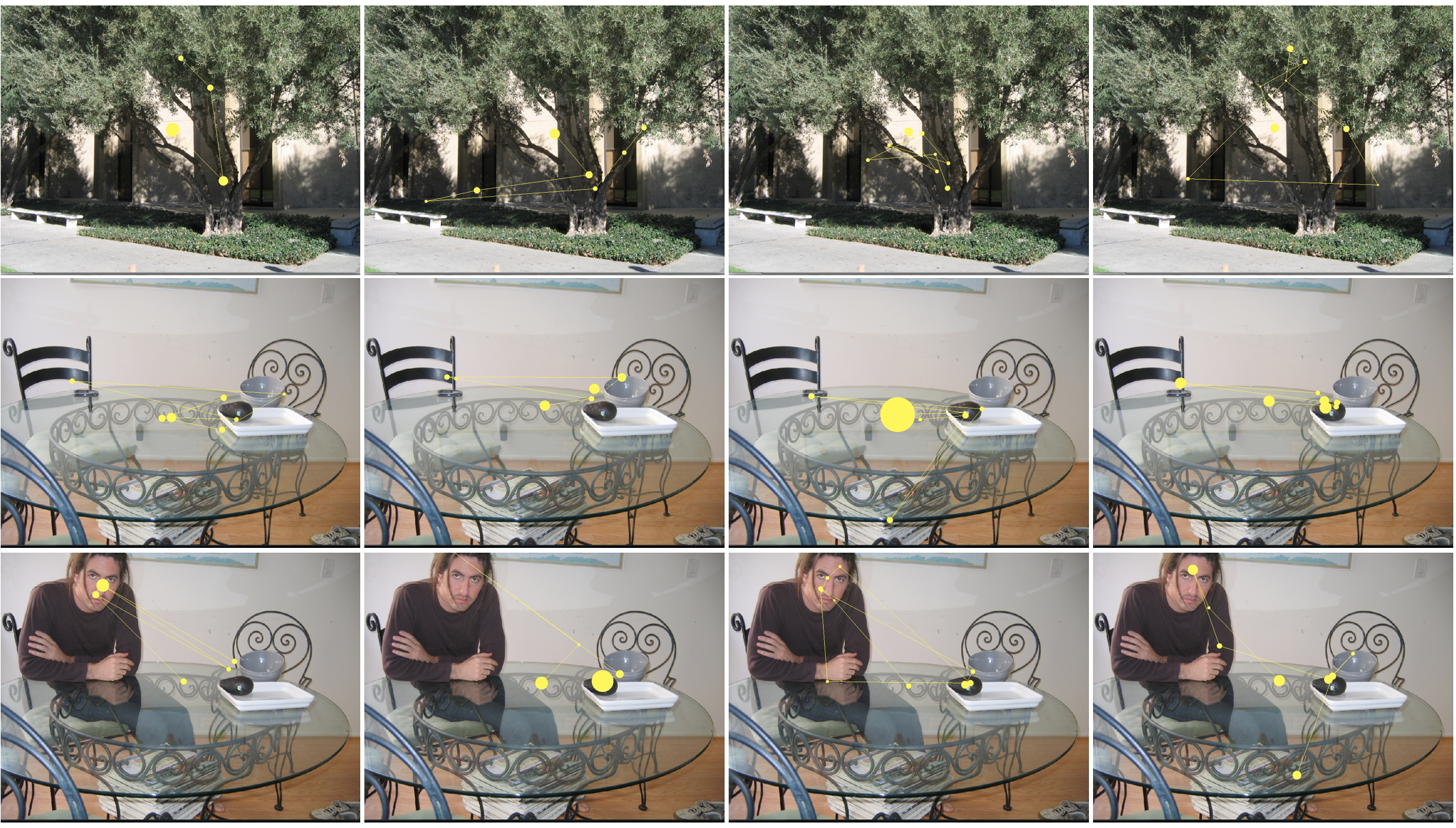
Figure 1: Scan paths eye tracked from different human observers while viewing three pictures of different information content: outdoor (top row), indoor with meaningful objects (middle row), indoor with high semantic content (person and face, bottom row). The area of yellow disks marking fixations between saccades is proportional to fixation time (images freely available from the Fixations in FAces dataset).

Under this conceptualization, when the input $\mathbf{I}$ is a static scene (a picture), the fixation duration time and saccade (lengths and directions) sequence are the only observables of the underlying guidance mechanism. When $\mathbf{I}$ stands for a time varying scene (e.g. a video), pursuit needs to be taken into account, too. We will adopt the generic terms of gaze shifts for either pursuit, saccades and fixational movements.

In the following, for notational simplicity, we will write the time series $\{\mathbf{r}_{F_{1}},t_{1};\mathbf{r}_{F_{2}},t_{2};\cdots\}$ as the sequence $\{\mathbf{r}_{F}(1),\mathbf{r}_{F}(2),\cdots\}$, unless the expanded form is needed. Also, we will generically refer to such sequence as scan path, though this term has a historically precise meaning in the eye movement literature [Privitera (2006)].

The common practice of computational approaches to derive the mapping (1) is to conceive it as a two step procedure:

1. obtaining a suitable perceptual representation $\mathcal{W}$, i.e., $\mathbf{I}\mapsto\mathcal{W}$;

2. using $\mathcal{W}$ to generate the scan path, $\mathcal{W}\mapsto\{\mathbf{r}_{F}(1),\mathbf{r}_{F}(2),\cdots\}$.

It is important to remark that each gaze position $\mathbf{r}_{F}(t)$ sets a new field of view for perceiving the world, thus $\mathcal{W}=\{\mathcal{W}_{\mathbf{r}_{F}(1)},\mathcal{W}_{\mathbf{r}_{F}(2)},\cdots\}$ should be a time-varying representation, even in the case of a static image input. This feedback effect of the moving gaze is hardly considered at the modelling stage [Zelinsky (2008), Tatler et al. (2011)].

By overviewing the field [Tatler et al. (2011), Borji and Itti (2013), Bruce et al. (2015), Bylinskii et al. (2015)], computational modelling has been mainly concerned with the first step: deriving a representation $\mathcal{W}$, typically in the form of a salience map. Yet, such step has recently evolved in a parallel research program, in which gaze shift prediction and simulation is not the focus, but salient object detection (for an in-depth review of this “second wave” of saliency-centered methods, see borji2014salient).

The second step, that is $\mathcal{W}\mapsto\{\mathbf{r}_{F}(1),\mathbf{r}_{F}(2),\cdots\}$, which actually brings in the question of how we look rather than where, is seldom taken into account. Surprisingly, in spite of the fact that the most cited work in the field [Itti et al. (1998)] clearly addressed the how issue (gaze shifts as the result of a WTA sequential selection of most salient locations), most models simply overlook the problem. As a matter of fact, the representation $\mathcal{W}$, once computed, is usually validated in respect of its capacity for predicting the image regions that would be explored by the overt attentional shifts of human observers (in a task designed to minimize the role of top-down factors). Predictability is assessed according to some established evaluation measures (see BorItti2012, and kummerer2015information, for a recent discussion).

In other cases, if needed for practical purposes, e.g. for robotic applications, the problem of oculomotor action selection is solved by adopting some simple deterministic choice procedure that usually relies on selecting the gaze position $\mathbf{r}$ as the argument that maximizes a measure on the given representation $\mathcal{W}$.

We will attack on the problem related to gaze shift generation in Sections 2.2 and 2.3. In the following Section we first discuss representational problems.

2.1 Levels of representation and control

The guidance of eye movements is likely to be influenced by a hierarchy of several interacting control loops, operating at different levels of processing. Each processing step exploits the most suitable representation of the viewed scene for its own level of abstraction. schutz2011eye, in a plausible portrayal, have sorted out the following representational levels: 1) salience, 2) objects, 3) values, and 4) plans.

Up to this date, the majority of computational models have retained a central place for low-level visual conspicuity [Tatler et al. (2011), Borji and Itti (2013), Bruce et al. (2015)]. The perceptual representation of the world $\mathcal{W}$ is usually epitomized in the form of a spatial saliency map, which is mostly derived bottom-up (early salience) following [Itti et al. (1998)].

The weakness of the bottom-up approach has been largely discussed (see, e.g. TatlerBallard2011eye,foulsham2008,EinhauserSpainPerona2008). Indeed, the effect of early salience on attention is likely to be a correlational effect rather than an causal one [Foulsham and Underwood (2008)], [Schütz et al. (2011)]. Few examples are provided in Fig. 2, where, as opposed to human scan paths (in free-viewing conditions), the scan path generated by using a salience-based representation [Itti et al. (1998)] does not spot semantically important objects (faces), the latter not being detected as regions of high contrast in colour, texture and luminance with respect to other regions of the picture.

Under these circumstances, early saliency can be modulated to improve its fixation prediction. Torralba has considered prior knowledge on the typical spatial location of the search target, as well as contextual information (the gist of a scene, rensink2000dynamic). Further, object knowledge can be used to top-down tune early salience. In particular, when dealing with faces, a face detection step [Cerf et al. (2008)], [deCroon et al. (2011)], [Marat et al. (2013)] or a prior for Bayesian integration with low level features [Boccignone et al. (2008)], can provide a reliable cue to complement early conspicuity maps. Indeed, faces drive attention in a direct fashion [Cerf et al. (2009)] and the same holds for text regions [Cerf et al. (2008), Clavelli et al. (2014)]. It has been argued that salience has only an indirect effect on attention by acting through recognised objects: observers attend to interesting objects and salience contributes little extra information to fixation prediction [Einhäuser et al. (2008)]. As a matter of fact, in the real world, most fixations are on task-relevant objects and this may or may not correlate with the saliency of regions of the visual array [Canosa (2009), Rothkopf et al. (2007)]. Notwithstanding, object-based information has been scarcely taken into account in computational models [Tatler et al. (2011)]. There are of course exceptions to this state of affairs, most notable ones those provided by Rao2002, Sun2008, the Bayesian models discussed by Poggio2010 and borji2012object.

The representational problem is just the light side of the eye guidance problem. When actual eye tracking data are considered, one has to confront with the dark side: regardless of the perceptual input, scan paths exhibit both systematic tendencies and notable inter- and intra-subject variability. As canosa2009real put it, where we choose to look next at any given moment in time is not completely deterministic, but neither is it completely random.

2.2 Biases in oculomotor behaviour

Systematic tendencies or “biases” in oculomotor behaviour can be thought of as regularities that are common across all instances of, and manipulations to, behavioural tasks [Tatler and Vincent (2008), Tatler and Vincent (2009)]. In that case case useful information about how the observers will move their eyes can be found. One remarkable example is the amplitude distribution of saccades and microsaccades that typically exhibit a positively skewed, long-tailed shape [Tatler et al. (2011), Dorr et al. (2010), Tatler and Vincent (2008), Tatler and Vincent (2009)]. Other paradigmatic examples of systematic tendencies in scene viewing are: initiating saccades in the horizontal and vertical directions more frequently than in oblique directions; small amplitude saccades tending to be followed by long amplitude ones and vice versa [Tatler and Vincent (2008), Tatler and Vincent (2009)].

Indeed, biases affecting the manner in which we explore scenes with our eyes are well known in the psychological literature (see le2016introducing for a thorough review), albeit underexploited in computational models. Such biases may arise from a number of sources. tatler2009prominence have suggested the following: biomechanical factors, saccade flight time and landing accuracy, uncertainty, distribution of objects of interest in the environment, task parameters.

Understanding biases in eye guidance can provide powerful new insights into the decision about where to look in complex scenes. In a remarkable study, tatler2009prominence provided striking evidence that a model based solely on these biases and therefore blind to current visual information can outperform salience-based approaches. Further, the predictive performance of a salience-based model can be improved from $56\%$ to $80\%$ by including the probability of gaze shift directions and amplitudes.

Failing to account properly for such characteristics results in scan patterns that are fairly different from those generated by human observers (which can be easily noticed in the example provided in Fig. 2) and eventually in distributions of saccade amplitudes and orientations that do not match those estimated from human eye behaviour.

2.3 Variability

When looking at natural images or movies [Dorr et al. (2010)] under a free-viewing or a general-purpose task, the relocation of gaze can be different among observers even though the same locations are taken into account. In practice, there is a small probability that two observers will fixate exactly the same location at exactly the same time. This effect is even more remarkable when free-viewing static images: consistency in fixation locations selected by observers decreases over the course of the first few fixations after stimulus onset [Tatler et al. (2011)] and can become idiosyncratic. Such variations in individual scan paths (as regards chosen fixations, spatial scanning order, and fixation duration) still hold when the scene contains semantically rich ”objects” (e.g., faces, see Figures 1 and 2). Variability is also exhibited by the same subject along different trials on equal stimuli.

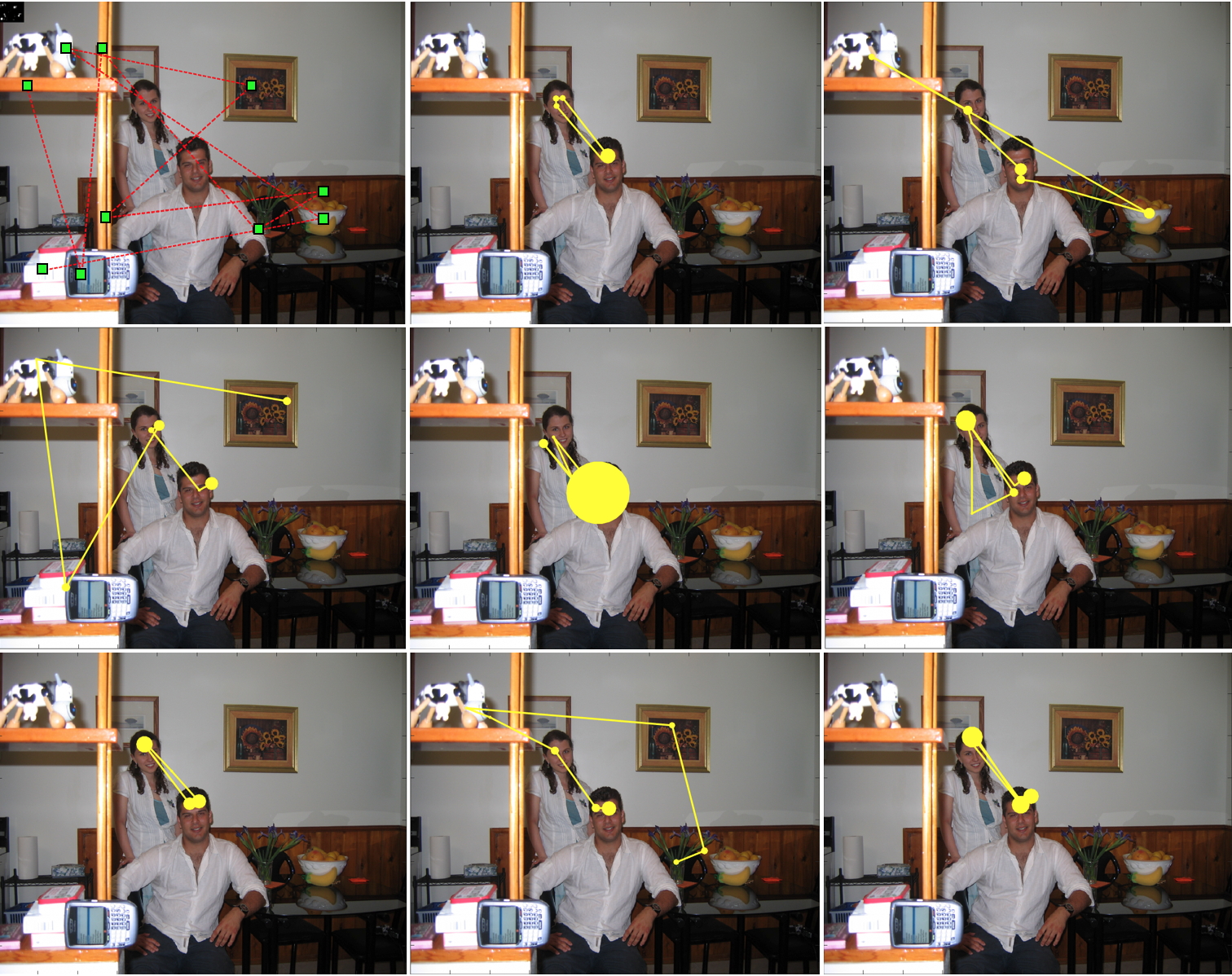
Figure 2: A worst case analysis of scan path generation based on early salience (top left image, via IttiKoch98) vs. scan paths eye tracked from human subjects. Despite of inter-subject variability concerning the gaze relocation pattern and fixation duration time, human observers consistently fixate on the two faces. The simulated scan path fails to spot such semantically important objects that have not been highlighted as regions of high contrast in colour, texture and luminance. The area of yellow disks marking human fixations is proportional to fixation time ( Fixations in FAces dataset).

Randomness in motor responses is likely to be originated from endogenous stochastic variations that affect each stage between a sensory event and the motor response: sensing, information processing, movement planning and executing [van Beers (2007)]. It is worth noting that uncertainty comes into play since the earliest stage of visual processing: the human retina evolved such that high quality vision is restricted to the small part of the retina (about $2^{0}-5^{0}$ degrees of visual angle) aligned with the visual axis, the fovea at the centre of vision. Thus, for many visually-guided behaviours the coarse information from peripheral vision is insufficient [Strasburger et al. (2011)]. In certain circumstances, uncertainty may promote almost “blind” visual exploration strategies [Tatler and Vincent (2009), Over et al. (2007)], much like the behaviour of a foraging animal exploring the environment under incomplete information; indeed when animals have limited information about where targets (e.g., resource patches) are located, different random search strategies may provide different chances to find them bartumeus2009optimal.

Indeed, few works have been trying to cope with the variability issue, after the early work by ellistark, hacisalihzade1992visual. The glorious WTA scheme [Itti et al. (1998)], or variants such as the selection of the proto-object with the highest attentional weight [Wischnewski et al. (2010)] are deterministic procedures. Even when probabilistic frameworks are used to infer where to look next, the final decision is often taken via the maximum a posteriori (MAP) criterion which again is a deterministic procedure (technically, an $\arg\max$ operation, see elazary2010bayesian,bocc08tcsvt,geisler2005,ChernyakStark), or variants like the robust mean (arithmetic mean with maximum value) over candidate positions [Begum et al. (2010)]. As a result, for a chosen visual input $\mathbf{I}$ the mapping $\mathcal{W}\mapsto\{\mathbf{r}_{F}(1),\mathbf{r}_{F}(2),\cdots\}$ will always generate the same scan path across different trials.

As a last remark, the variability of visual scan paths has been considered a nuisance rather than an opportunity from a modelling standpoint. Nevertheless, beside theoretical relevance for modelling human behavior, the randomness of the process can be an advantage in computer vision and learning tasks. For instance, martinezLungarella have reported that a stochastic attention selection mechanism (a refinement of the algorithm proposed in bfpha04) enables the i-Cub robot to explore its environment up to three times faster compared to the standard WTA mechanism [Itti et al. (1998)]. Indeed, stochasticity makes the robot sensitive to new signals and flexibly change its attention, which in turn enables efficient exploration of the environment as a basis for action learning [Nagai (2009b), Nagai (2009a)].

There are few notable exceptions to this current state of affairs, which will be discussed in Section 3.1.

3 Framing models in a probabilistic setting

We contend with the above issues by stating that observables such as fixation duration and gaze shift lengths and directions are random variables (RVs) that are generated by an underlying stochastic process. In other terms, the sequence $\{\mathbf{r}_{F}(1),\mathbf{r}_{F}(2),\cdots\}$ is the realization of a stochastic process, and the ultimate goal of a computational theory is to develop a mathematical model that describes statistical properties of eye movements as closely as possible. The problem of answering the question Where to Look Next? in a formal way can be conveniently set in a probabilistic Bayesian framework. tatler2009prominence have re-phrased this question in terms of the posterior probability density function (pdf) $P(\mathbf{r}\mid\mathcal{W})$, which accounts for the plausibility of generating the gaze shift $\mathbf{r}=\mathbf{r}_{F}(t)-\mathbf{r}_{F}(t-1)$, after the perceptual evaluation $\mathcal{W}$. Formally, via Bayes’ rule:

$$P(\mathbf{r}\mid\mathcal{W})=\frac{P(\mathcal{W}\mid\mathbf{r})}{P(\mathcal{W})}P(\mathbf{r}).$$ (2)

In Eq. 2, the first term on the r.h.s. accounts for the likelihood $P(\mathcal{W}\mid\mathbf{r})$ of $\mathbf{r}$ when visual data (e.g., features, such as edges or colors) are observed under a gaze shift $\mathbf{r}_{F}(t)\rightarrow\mathbf{r}_{F}(t+1)$, normalized by $P(\mathcal{W})$, the evidence of the perceptual evaluation. As they put it, “The beauty of this approach is that the data could come from a variety of data sources such as simple feature cues, derivations such as Itti’s definition of salience, object-or other high-level sources”. The second term is the pdf $P(\mathbf{r})$ incorporating prior knowledge on gaze shift execution.

The generative model behind Eq. 2 is shown in Fig. 4 shaped in the form of a Probabilistic Graphical Model (PGM, see murphy2012machine for an introduction). A PGM is a graph where nodes (e.g., $\mathbf{r}$ and $\mathcal{W}$) denote RVs and directed arcs (arrows) encode conditional dependencies between RVs, e.g $P(\mathcal{W}\mid\mathbf{r})$. A node with no input arcs (for example $\mathbf{r}$) is associated with a prior probability, e.g., $P(\mathbf{r})$. Technically, as a whole, the PGM specifies at a glance a chosen factorization of the joint probability of all nodes. Thus, in Fig. 4 we can promptly read that $P(\mathcal{W},\mathbf{r})=P(\mathcal{W}\mid\mathbf{r})P(\mathbf{r})$. The PGM in Fig. 4 represents the PGM in Fig. 4, but unrolled in time. Note that now the arc $\mathbf{r}_{F}(t)\rightarrow\mathbf{r}_{F}(t+1)$ makes explicit the dynamics of the gaze shift occurring with probability $P(\mathbf{r}_{F}(t+1)\mid\mathbf{r}_{F}(t))$.

Figure 3: The generative model in PGM form supporting the Bayesian inference specified via Eq 2

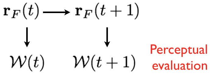
Figure 4: The dynamic PGM obtained by unrolling in time the PGM depicted in Fig. 4

The probabilistic model represented in Fig. 4 is generative in the sense that if all pdfs involved were fully specified, the attentive process could be simulated (via ancestral sampling, murphy2012machine) as:

1. Sampling the gaze shift from the prior:

   $$\mathbf{r}^{*}\sim P(\mathbf{r});$$ (3)

2. Sampling the observation of the world under the gaze shift:

   $$\mathcal{W}^{*}\sim P(\mathcal{W}\mid\mathbf{r}^{*}).$$ (4)

Inferring the gaze shift $\mathbf{r}$ when $\mathcal{W}$ is known boils down to the inverse probability problem (inverting the arrows), which is solved via Bayes’ rule (Eq. 2). In the remainder of this paper we will largely use PGMs to simplify the presentation and discussion of probabilistic models.

We will see in brief (Section 3.2) that many current approaches previously mentioned can be accounted for by the likelihood term alone. But, crucial, and related to issues raised in Section 2.2, is the Bayesian prior $P(\mathbf{r})$.

3.1 The prior, first

The prior $P(\mathbf{r})$ can be defined prima facie as the probability of shifting the gaze to a location irrespective of the visual information at that location, although the term “irrespective” should be used with some caution [Le Meur and Coutrot (2016)]. Indeed, the prior is apt to encapsulate any systematic tendency in the manner in which we explore scenes with our eyes. The striking result obtained by tatler2009prominence is that if we learn $P(\mathbf{r})$ from the actual observer’s behavior, then we can stochastically sample gaze shifts (Eq. 3) so to obtain scan paths that, blind to visual information, out-perform feature-based accounts of eye guidance.

Note that the apparent simplicity of the prior term $P(\mathbf{r})$ hides a number of subtleties. For instance, Tatler and Vincent expand the random vector $\mathbf{r}$ in terms of its components, amplitude $l$ and direction $\theta$. Thus, $P(\mathbf{r})=P(l,\theta)$. This simple statement paves the way to different options.

First easy option: such RVs are marginally independent, thus, $P(l,\theta)=P(l)P(\theta)$. In this case, gaze guidance, solely relying on biases, could be simulated by expanding Eq. 3 via independent sampling of both components, i.e. at each time $t$, $l(t)\sim P(l(t)),\theta(t)\sim P(\theta(t))$. Alternative option: conjecture some kind of dependency, e.g. amplitude on direction so that $P(l,\theta)=P(l\mid\theta)P(\theta)$. In this case, the gaze shift sampling procedure would turn into the sequence $\widehat{\theta}(t)\sim P(\theta(t)),l(t)\sim P(l(t)\mid\widehat{\theta}(t))$. Further: assume that there is some persistence in the direction of the shift, which give rise to a stochastic process in which subsequent directions are correlated, i.e., $\theta(t)\sim P(\theta(t)\mid\theta(t-1))$, and so on.

To summarize, by simply taking into account the prior $P(\mathbf{r})$, a richness of possible behaviors and analyses are brought into the game. Unfortunately, most computational accounts of eye movements and visual attention have overlooked this opportunity, with some exceptions. For instance, tavakoli2013stochastic propose a system model for saccade generation in a stochastic filtering framework. A prior on amplitude $P(l(t))$ is considered by learning a Gaussian mixture model from eye tracking data. This way one aspect of biases is indirectly taken into account. It is not clear if their model accounts for variability and whether and how oculomotor statistics compare to human data. In [Kimura et al. (2008)], simple eye-movements patterns are straightforwardly incorporated as a prior of a dynamic Bayesian network to guide the sequence of eye focusing positions on videos.

In a different vein, le2016introducing have recently addressed in-depth the bias problem and made the interesting point that viewing tendencies are not universal, but modulated by the semantic visual category of the stimulus. They learn the joint pdf $P(l,\theta)$ of saccade amplitudes and orientations via kernel density estimation; fixation duration is not taken into account. The model also brings in variability [Le Meur and Liu (2015)] by generating a number $N_{c}$ of random locations according to conditional probability $P(\mathbf{r}_{F}(t)\mid\mathbf{r}_{F}(t-1))$ and the location with the highest saliency gain is chosen as the next fixation point. $N_{c}$ controls the degree of stochasticity.

Others have tried to capture eye movements randomness [Keech and Resca (2010), Rutishauser and Koch (2007)] but limiting to specific tasks such as conjunctive visual search. A few more exceptions can be found, but only in the very peculiar field of eye-movements in reading (see feng2006eye, for a discussion).

The variability and bias issues have been explicitly addressed from first principles in the theoretical context of Lévy flights [Brockmann and Geisel (2000), Boccignone and Ferraro (2004)]. The perceptual component was limited to a minimal core (e.g., based on a bottom-up salience map) sufficient enough to support the eye guidance component. In particular in [Boccignone and Ferraro (2004)] the long tail, positively skewed distribution of saccade amplitudes was shaped as a prior in the form of a Cauchy distribution, whilst randomness was addressed at the algorithmic level by prior sampling $\mathbf{r}\sim P(\mathbf{r}(t))$ followed by a Metropolis-like acceptance rule based on a deterministic saliency potential field. The degree of stochasticity was controlled via the “temperature” parameter of the Metropolis algorithm. The underlying eye guidance model was that of a random walker exploring the potential landscape (salience) according to a Langevin-like stochastic differential equation (SDE). The merit of such equation is the joint treatment of both the deterministic and the stochastic (variability) components behind eye guidance.

This basic mechanism has been refined and generalized in [Boccignone and Ferraro (2013)] to composite $\alpha$-stable or Lévy random walks (the Cauchy law is but one instance of the class of $\alpha$-stable distributions), where, inspired by animal foraging behaviour, a twofold regime can be distinguished: local exploitation (fixational movements following Brownian motion) and large exploration/relocation (saccade following Lévy motion). What is interesting, with respect to the early model [Boccignone and Ferraro (2004)], is that the choice between the “feed” or “fly” states is made by sampling from a Bernoulli distribution, $Bern(z\mid\pi)$, with the parameter $\pi$ sampled from the conjugate prior $Beta(\pi\mid\alpha,\beta)$. In turn, the behaviour of the Beta prior can be shaped via its hyperparameters $(\alpha,\beta)$, which, in an Empirical Bayes approximation, can be tuned as a function of the class of perceptual data at hand (in the vein of le2016introducing) and of time spent in feeding (fixation duration). Most important, this approach paves the way to the possibility of treating visual exploration strategies in terms of foraging strategies [Wolfe (2013), Cain et al. (2012), Boccignone and Ferraro (2014), Clavelli et al. (2014), Napoletano et al. (2015)]. We will further expand on this in Section 4.

3.2 The unbearable lightness of the likelihood

We noticed before, by inspecting Eq. 2 that the term $\frac{P(\mathcal{W}\mid\mathbf{r})}{P(\mathcal{W})}$ could be related to many models proposed in the literature. This is an optimistic view. Most of the approaches actually discard the dynamics of gaze shifts implicitly captured by the shift vector $\mathbf{r}(t)$. In practice, they are more likely to be described by a simplified version of Eq. 2:

$$P(\mathbf{r}_{F}\mid\mathcal{W})=\frac{P(\mathcal{W}\mid\mathbf{r}_{F})}{P(\mathcal{W})}P(\mathbf{r}_{F}).$$ (5)

The difference between Eq. 2 and 5 is subtle. The posterior $P(\mathbf{r}_{F}\mid\mathcal{W})$ now answers the query “What is the probability of fixating at location $\mathbf{r}_{F}$ given visual data $\mathcal{W}$?” Further, the prior $P(\mathbf{r}_{F})$ simply accounts for the probability of spotting location $\mathbf{r}_{F}$. As a matter of fact, Eq. 5 bears no dynamics.

In probabilistic terms we may re-phrase this result as the outcome of an assumption of independence: $P(\mathbf{r})=P(\mathbf{r}_{F}(t)-\mathbf{r}_{F}(t-1))\simeq P(\mathbf{r}_{F}(t)\mid\mathbf{r}_{F}(t-1))=P(\mathbf{r}_{F}(t))$. To make things even clearer, let us explicitly substitute $\mathbf{r}_{F}$ with a RV $\mathbf{L}$ denoting locations in the scene, and $\mathcal{W}$ with RV $\mathbf{F}$ denoting features (whatever they may be); then, Eq. 5 boils down to

$$P(\mathbf{L}\mid\mathbf{F})=\frac{P(\mathbf{F}\mid\mathbf{L})}{P(\mathbf{F})}P(\mathbf{L}).$$ (6)

The PGM underlying this inferential step is a very simple one and is represented in Figure 8. A straightforward but principled use of Eq. 6, which has been exploited by approaches that draw upon techniques borrowed from statistical machine learning [Murphy (2012)] is the following: consider $\mathbf{L}$ as a binary RV taking values in $\left[0,1\right]$ (or $\left[-1,1\right]$), so that $P(\mathbf{L}=1\mid\mathbf{F})$ represents the probability for a pixel, a superpixel or a patch of being classified as salient.

Figure 5: PGM representing a feature-based perceptual evaluation component $\mathcal{W}$

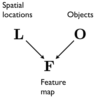
Figure 6: PGM representing a object-based perceptual evaluation component $\mathcal{W}$ [Torralba et al. (2006)]

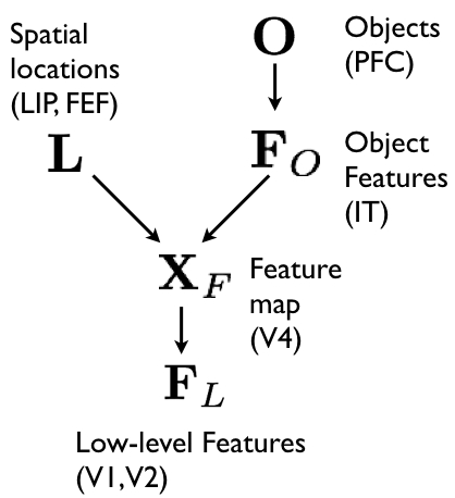
Figure 7: The Bayesian model by Poggio2010, which maps the PGM structure to brain areas underpinning visual attention: early visual areas V1 and V2, V4, lateral intraparietal (LIP), frontal eye fields (FEF), inferotemporal (IT), prefrontal cortex (PFC)

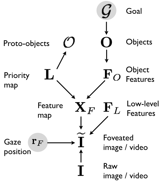
Figure 8: An extension of the PGM by Poggio2010, cfr. Fig. 8, adopted in [Clavelli et al. (2014)] and [Napoletano et al. (2015)]. In this case $\mathcal{W}$ explicitly depends on the current gaze position $\mathbf{r}_{F}$ and goal $\mathcal{G}$.

In the case the prior $P(\mathbf{L})$ is assumed to be uniform (no spatial bias, no preferred locations), then $P(\mathbf{L}=1\mid\mathbf{F})\simeq P(\mathbf{F}\mid\mathbf{L}=1)$. The likelihood function $P(\mathbf{F}\mid\mathbf{L}=1)$ can be determined in many ways; e.g., nonparametric kernel density estimation has been addressed by seo2009, who use center / surround local regression kernels for computing $\mathbf{F}$.

More generally, taking into account the ratio $f(\mathbf{L})=\frac{P(\mathbf{L}=1\mid\mathbf{F})}{P(\mathbf{L}=0\mid\mathbf{F})}$ (or, commonly, the log-ratio) casts the saliency detection problem in a classification problem, in particular a discriminative one [Murphy (2012)], for which a variety of learning techniques are readily available. kienzle2006nonparametric pioneered this approach by learning the saliency discriminant function $f(\mathbf{L})$ directly from human eye tracking data using a support vector machine (SVM). Their approach has paved the way to a relevant number of works from [Judd et al. (2009)] – who trained a linear SVM from human fixation data using a set of low, middle and high-level features to define salient locations–, to most recent ones that wholeheartedly endorse machine learning trends. Henceforth, methods have been proposed relying on sparse representation of “feature words” (atoms) encoded in salient and non-salient dictionaries; these are either learned from local image patches [Yan et al. (2010), Lang et al. (2012)] or from eye tracking data of training images [Jiang et al. (2015)]. Graph-based learning is one other trend, from the seminal work of harel2007graph to yu2014maximal (see the latter, for a brief review of this field). Crucially, for the research practice, data-driven learning methods allow to contend with large scale dynamic datasets. mathe2015actions in the vein of kienzle2006nonparametric and judd2009learning use SVM, but they remarkably exploit state-of-the art computer vision datasets (Hollywood-2 and UCF Sports) annotated with human eye movements collected under the ecological constraints of a visual action recognition task.

As a general comment on (discriminative) machine learning-based methods, on the one hand it is embraceable the criticism by BorItti2012, who surmise that these techniques make “models data-dependent, thus influencing fair model comparison, slow, and to some extent, black-box.” But on the other hand, one important lesson of these approaches lies in that they provides a data-driven way of deriving the most relevant visual features as optimal predictors. The learned patterns can shape receptive fields (filters) that have equivalent or superior predictive power when compared against hand-crafted (and sometimes more complicated) models [Kienzle et al. (2009)]. Certainly, this lesson is at the base of the current exponentially growth of methods based on deep learning techniques [LeCun et al. (2015)], in particular Convolutional Neural Networks (CNN, cfr. deepTaxonomy2016 for a focused review), where the computed features seem to outperform, at least from an engineering perspective, most of, if not all, the state-of-the art features conceived in computer vision.

Again, CNNs, as commonly exploited in the current practice, bring no significant conceptual novelty as to the use of Eq. 6: fixation prediction is formulated as a supervised binary classification problem (in some case, regression is addressed, wang2016deep). For example, vig2014large use a linear SVM for learning the saliency discriminant function $f(\mathbf{L})$ after a large-scale search for optimal features $\mathbf{F}$. Similarly, shenZhao2014learning detect salient region via linear SVM fed with features computed from multi-layer sparse network model. [Lin et al. (2014)] use the simple normalization step [Itti et al. (1998)] to approximate $P(\mathbf{L}=1\mid\mathbf{F})$, where [Kruthiventi et al. (2015)] use the last $1\times 1$ convolutional layer of a fully convolutional net. Cogent here is the outstanding performance of CNN in learning and representing features that correlate well with eye fixations, like objects, faces, context.

Clearly, one problem is the enormous amount of training data necessary to train these networks, and the engineering expertise required, which makes them difficult to apply for predicting saliency. However, kummerer2014deep by exploiting the well known network from [Krizhevsky et al. (2012)] as starting point, have given evidence that deep CNN trained on computer vision tasks like object detection boost saliency prediction. The network by AlexNetNIPS2012 has been optimized for object recognition using a massive dataset consisting of more than one million images, and results reported by kummerer2014deep on static pictures are impressive when compared to state-of-the-art methods, even to previous CNN-based proposals [Vig et al. (2014)].

Apart from the straightforward implementation via popular machine-learning algorithms, the “light” model described by Eq. 6 is further amenable to a minimal model, which, surprisingly enough, is however capable of accounting for a large number of approaches. This can be easily appreciated by setting $P(\mathbf{F}\mid\mathbf{L})=const.,P(\mathbf{L})=const.$ so that Eq. 6 reduces to

$$P(\mathbf{L}\mid\mathbf{F})\propto\frac{1}{P(\mathbf{F})}.$$ (7)

Eq. 7 states that the probability of fixating a spatial location $\mathbf{L}=(x,y)$ is higher when “unlikely” features (unlikeliness $\approx\frac{1}{P(\mathbf{F})}$) occur at that location. In a natural scene, it is typically the case of high contrast regions (with respect to either luminance, color, texture or motion). This is nothing but the salience-based component of the most prominent model in the literature [Itti et al. (1998)], which Eq. 7 re-phrases in probabilistic terms.

A thorough reading of the review by BorItti2012 is sufficient to gain the understanding that a great deal of computational models so far proposed (47 over 63 models) are much or less variations of this theme (albeit experimenting with different features, different weights for combining them, etc.) even when sophisticated probabilistic techniques are adopted to shape the distribution $P(\mathbf{F})$ (e.g., nonparametric Bayes techniques, BoccICPR08). Clearly, there are works that have tried to avoid weaknesses related to such a light-modelling of the perceptual input, and have tried to climb up the levels of the representation hierarchy [Schütz et al. (2011)]. Some examples are summarized at a glance in Figure 8 (but see BorItti2012).

Nevertheless, in spite of its simplicity, Eq. 7 is apt to pave the way to interesting frameworks. For instance, by noting that $\log\frac{1}{P(\mathbf{F})}$ is nothing but Shannon’s Self- Information, information theoretic approaches become available at the algorithmic level. These approaches set computational constraints under the general assumption that saliency computation serves to maximize information sampled from the environment [Bruce and Tsotsos (2009)].

Keeping on with the information theory framework, and going back to Eq. 6, a simple manipulation,

$$\log P(\mathbf{L}\mid\mathbf{F})-\log P(\mathbf{L})=\log\frac{P(\mathbf{F}\mid\mathbf{L})}{P(\mathbf{F})}$$ (8)

sets the focus on the discrepancy, or dissimilarity, $\log P(\mathbf{L}\mid\mathbf{F})-\log P(\mathbf{L})=\log\frac{P(\mathbf{L}\mid\mathbf{F})}{P(\mathbf{L})}$ between the log-posterior and the log-prior. A (non-commutative) measure, formalizing this notion of dissimilarity is readily available in information theory, namely the Kullback-Leibler (K-L) divergence between two distributions $P(X)$ and $Q(X)$ [MacKay (2002)]:

$$D_{KL}(P(X)||Q(X))=\int_{X}\log\frac{P(x)}{Q(x)}P(x)dx$$ (9)

Measuring differences between posterior and prior beliefs of the observers is however a general concept applicable across different levels of abstraction. For instance, one might consider the object-based model [Torralba et al. (2006)] in Fig. 8, which can be used for inferring the joint posterior of gazing at certain kinds of objects $\mathbf{O}$ at location $\mathbf{L}$ of a viewed scene, namely, $P(\mathbf{O},\mathbf{L}\mid\mathbf{F})\propto P(\mathbf{F}\mid\mathbf{O},\mathbf{L})P(\mathbf{O},\mathbf{L})$. Then, $D_{KL}(P(\mathbf{O},\mathbf{L}\mid\mathbf{F})||P(\mathbf{O},\mathbf{L}))$ is the average of the log-odd ratio, measuring the divergence between observer’s prior belief distribution on $(\mathbf{O},\mathbf{L})$ and his posterior belief distributions after perceptual data $\mathbf{F}$ have been gathered. Indeed, this is a statement that can be generalized to any model $\mathbf{M}$ in a model space $\mathcal{M}$ and new data observation $\mathbf{D}$ so to define the Bayesian surprise [Baldi and Itti (2010)] $\mathcal{S}(\mathbf{D},\mathbf{M})$: $\mathbf{D}$ is surprising if the posterior distribution resulting from observing $\mathbf{D}$ significantly differs from the prior distribution, i.e., $S(\mathbf{D},\mathbf{M})=D_{KL}(P(\mathbf{M}\mid\mathbf{D})||P(\mathbf{M}))$. itti2009bayesian have shown that Bayesian surprise attracts human attention in dynamic natural scenes. To recap, Bayesian surprise is a measure of salience based on the K–L divergence.

Eventually, note that the K-L divergence (9) is a flexible tool and can be used for different purposes. For instance, when dealing with models of perceptual evaluation such as those specified in Figs 8, 8, and 8, once the model has been detailed at the computational theory level via its PGM, then using the latter for learning inference and prediction brings in the algorithmic level. Indeed, for any Bayesian generative model other than trivial ones, such steps are usually performed in approximate form [Murphy (2012)]. Stochastic approximation resorting to algorithms such as Markov-chain Monte Carlo (MCMC) and Particle Filtering (PF) is one possible choice; the alternative choice is represented by deterministic optimization algorithms [Murphy (2012)] such as variational Bayes (VB) or belief propagation (BP, a message passing scheme exchanging beliefs between PGM nodes). For example, the model by Poggio2010, following the work of rao2005, relies upon BP message passing for inferential steps. Interestingly enough, rao2005 has argued for a plausible neural implementation of BP. VB algorithms, on the other hand, are based on Eq. 9, where $P$ usually stands for a complete distribution and $Q$ is the approximating distribution; then, parameter (or model) learning is accomplished by minimizing the K-L divergence (as an example, the well known Expectation-Maximization algorithm, EM, can be considered a specific case of the VB algorithm, Mackay,murphy2012machine). In Section 4 we will also touch on a deeper interpretation of the K-L minimization / VB algorithm.

But at this point a simple question arises: where have the eye movements gone?

4 Making a step forward: back to the beginning of active vision

Visual perception coupled with gaze shifts should be considered the Drosophila of perception-action loops. Among the variety of active behaviors the organism can fluently engage to purposively act upon and perceive the world (e.g, moving the body, turning the head, manipulating objects), oculomotor behavior is the minimal, least energy, unit. To perform $3$-$4$ saccades per second, the organism roughly spends $300$ msecs to close the loop ($200$ msecs for motor preparation and execution, $100$ msecs left for perception).

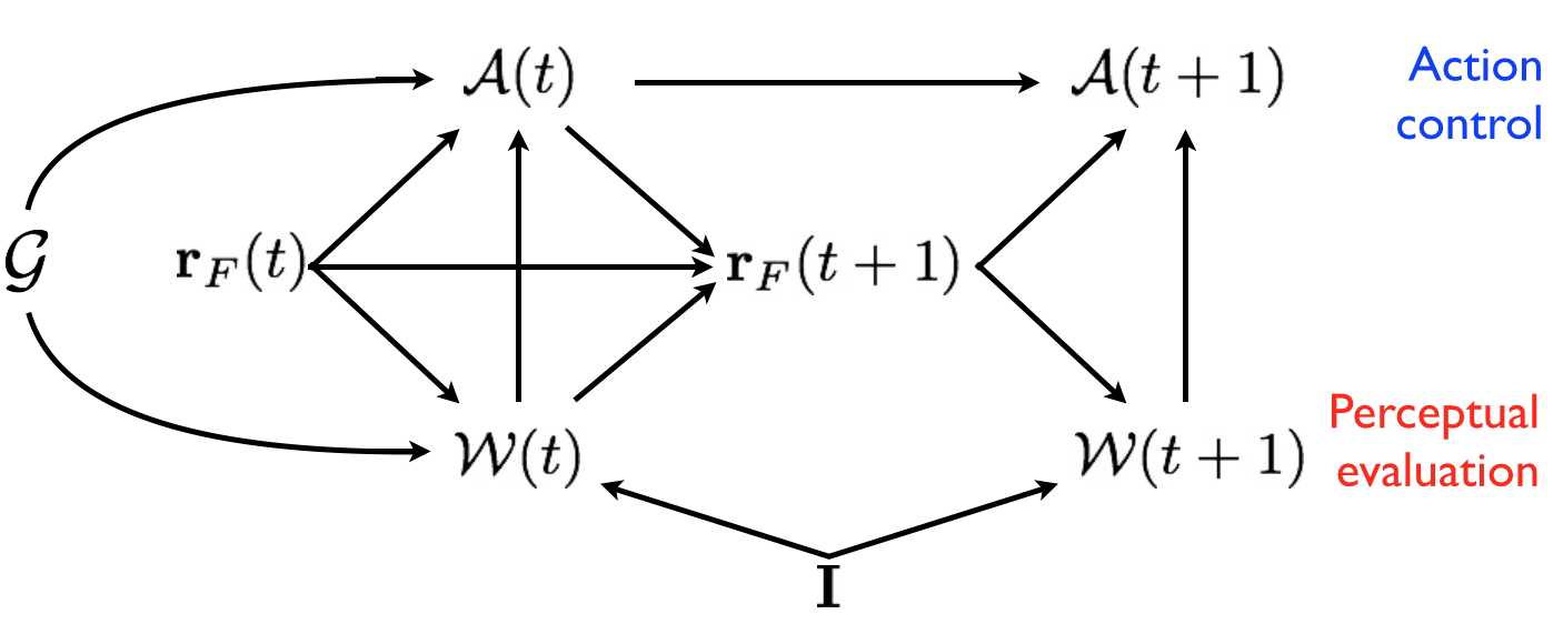
Figure 9: The perception-action loop unfolded in time as a dynamic PGM. $\mathcal{A}(t)$ denotes the ensemble of time-varying RVs defining the oculomotor action setting; $\mathcal{W}(t)$ stands for the ensemble of time-varying RVs characterising the scene as actively perceived by the observer; $\mathcal{G}$ summarizes the given goal(s), To simplify the graphics, conditional dependencies $\mathcal{G}\rightarrow\mathcal{A}(t+1)$ and $\mathcal{G}\rightarrow\mathcal{W}(t+1)$ have been omitted.

One way to make justice of this forgotten link is going back to first principles by re-shaping the problem as the action-perception loop, which is presented in Figure 9 in the form of a dynamic PGM. The model relies upon the following assumptions:

• The scene that will be perceived at time $t+1$, namely $\mathcal{W}(t+1)$ is inferred from the raw data $\mathbf{I}$, gazed at $\mathbf{r}_{F}(t+1)$, under the goal $\mathcal{G}$ assigned to the observer, and is conditionally dependent on current perception $\mathcal{W}(t)$. Thus, the perceptual inference problem is summarised by the conditional distribution $P(\mathcal{W}(t+1)|\mathcal{W}(t),\mathbf{r}_{F}(t+1),\mathbf{I},\mathcal{G})$;

• The external goal $\mathcal{G}$ being assigned, the oculomotor action setting at time $t+1$, $\mathcal{A}(t+1)$, is drawn conditionally on current action setting $\mathcal{A}(t)$ and the perceived scene $\mathcal{W}(t+1)$ under gaze position $\mathbf{r}_{F}(t+1)$; thus, its evolution in time is inferred according to the conditional distribution $P(\mathcal{A}(t+1)|\mathcal{A}(t),\mathcal{W}(t+1),\mathbf{r}_{F}(t+1),\mathcal{G})$.

Note that the action setting dynamics $\mathcal{A}(t)\rightarrow\mathcal{A}(t+1)$ and the scene perception dynamics $\mathcal{W}(t)\rightarrow\mathcal{W}(t+1)$ are intertwined with one another by means of the gaze shift process $\mathbf{r}_{F}(t)\rightarrow\mathbf{r}_{F}(t+1)$: on the one hand next gaze position $\mathbf{r}_{F}(t+1)$ is used to define a distribution on $\mathcal{W}(t+1)$ and $\mathcal{A}(t+1)$; meanwhile, the probability distribution of $\mathbf{r}_{F}(t+1)$ is conditioned on current gaze position, $\mathcal{W}(t)$ and $\mathcal{A}(t)$, namely $P(\mathbf{r}_{F}(t+1)|\mathcal{A}(t),\mathcal{W}(t),\mathbf{r}_{F}(t))$.

We have previously discussed the perceptual evaluation component $\mathcal{W}(t)$. A general way of defining the oculomotor executive control component $\mathcal{A}(t)$ is through the following ensemble of RVs:

• $\{\mathbf{V}(t),\mathbf{R}(t)\}$: $\mathbf{V}(t)$ is a spatially defined RV used to provide a suitable probabilistic representation of value; $\mathbf{R}(t)$ is a binary RV defining whether or not a payoff (either positive or negative) is returned;

• $\{\pi(t),z(t),\xi(t)\}$: an oculomotor state representation as defined via the multinomial RV $z(t)$, occurring with probability $\pi(t)$, and determining the choice of motor parameters $\xi(z,t)$ guiding the actual gaze relocation (e.g., lenght and direction of a saccade as opposed to those driving a smooth pursuit) ;

• $\mathcal{D}(t)$: a set of state-dependent statistical decision rules to be applied on a set of candidate new gaze locations $\mathbf{r}_{new}(t+1)$ distributed according to the posterior pdf of $\mathbf{r}_{F}(t+1)$.

In the end, the actual shift can be summarised as the statistical decision of selecting a particular gaze location $\mathbf{r}^{\star}_{F}(t+1)$ on the basis of $P(\mathbf{r}_{F}(t+1)|\mathcal{A}(t),\mathcal{W}(t),\mathbf{r}_{F}(t))$ so to maximize the expected payoff under the current goal $\mathcal{G}$, and the action/perception cycle boils down to the iteration of the following steps:

1. Sampling the gaze-dependent current perception:

   $$\mathcal{W}^{*}(t)\sim P(\mathcal{W}(t)|\mathbf{r}_{F}(t),\mathbf{F}(t),\mathbf{I}(t),\mathcal{G});$$ (10)

2. Sampling the appropriate motor behavior (e.g., fixation or saccade):

   $$\mathcal{A}(t)^{*}\sim P(\mathcal{A}(t)|\mathcal{A}(t-1),\mathcal{W}^{*}(t),\mathcal{G});$$ (11)

3. Sampling where to look next:

   $$\mathbf{r}_{F}(t+1)\sim P(\mathbf{r}_{F}(t+1)|\mathcal{A}(t)^{*},\mathcal{W}^{*}(t),\mathbf{r}_{F}(t)).$$ (12)

It is worth noticing that we have chosen to describe the observer’s action / perception cycle in terms of stochastic sampling based on the probabilistic model in Figure 9. However, one can recast the inferential problems in terms of deterministic optimization: in brief, optimising the probabilistic model $\mathcal{W}$ of how sensations are caused, so that the resulting predictions can select the optimal $\mathcal{A}$ to guide active sampling (gaze shift) of sensory data. One such approach, which is well known in theoretical neuroscience but, surprisingly, hitherto unconsidered in computer vision, relies on the free-energy principle [Friston (2010), Feldman and Friston (2010), Friston et al. (2013)]. Free-energy $\mathcal{F}$ is a quantity from statistical physics and information theory [MacKay (2002)] that bounds the negative log-evidence of sensory data. Under simplifying assumptions, it boils down to the amount of prediction error of sensory data under a model. In such context, the action / perception cycle is the result of a dual minimization process: i) action reduces $\mathcal{F}$ by changing sensory input, namely by sampling (via gaze shifts) what one expects consistent with perceptual inferences; ii) perception reduces $\mathcal{F}$ by making inferences about the causes of sampled sensory signals and changing predictions. Friston defines this process “active inference”. To make a connection with Section 3.2, by minimizing the free-energy, Bayesian surprise is maximised; indeed, in Bayesian learning, free energy minimization is a common rationale behind many optimisation techniques such as VB and BP [MacKay (2002), Murphy (2012)]

The sampling scheme proposed is a general one and can be instantiated in different ways. For instance, in [Boccignone and Ferraro (2014)] the sampling step of Eq. 12 is performed through a generalization of the Langevin SDE equation used in [Boccignone and Ferraro (2013)]. Biases and variability are accounted for by the stochastic component of the equation. Since dealing with image sequences, the SDE provides operates in different dynamic modes: pursuit needs to be taken also into account in addition to saccades and fixational movements. Each mode is governed by a specific set of parameters of the $\alpha$-stable distribution estimated from eye tracking data. The choice among modes is accomplished by generalizing the method proposed in [Boccignone and Ferraro (2014)], using a Multinoulli distribution on $z(t)$ and with parameters $\pi(t)$ sampled from the conjugate prior, the Dirichlet distribution. In addition, the sampling step is used to accomplish an internal simulation step, where a number of candidates shifts is proposed and the most convenient is selected according to a decision rule. Also, the gaze dependent perception $\mathcal{W}$ can be modeled at any level of complexity (cfr. example in Figure 13, Section 5). In BocFerSMCB2013 it is based on proto-objects sampled from time-varying saliency. Figure 10 shows an excerpt of typical results of the model simulation, which compares human variability in gazing (top row) with that of two “simulated observers” (bottom rows) while viewing the monica03 clip from the CRCNS eye-1 dataset.

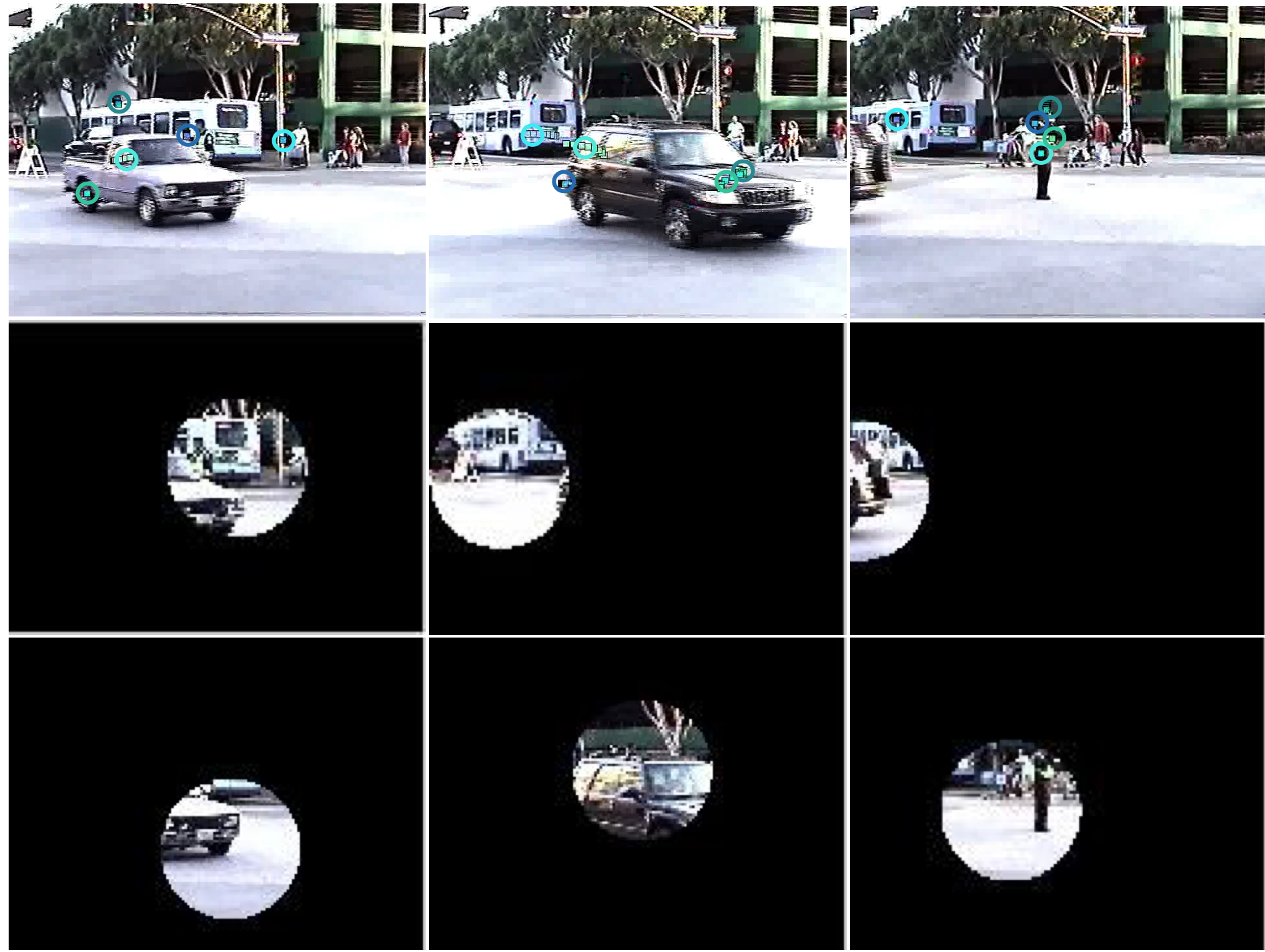
Figure 10: Top row: gaze positions (centers of the enhanced colored circles ) recorded from different observers on different frames of the monica03 clip from the CRCNS eye-1 dataset, University of South California (freely available online). Middle and bottom rows show, on the same frames, the fovea position of two “observers” simulated by the method described in [Boccignone and Ferraro (2014)].

In BocCOGN2014 and napboc_TIP2015 the perceptual evaluation component is extended to handle objects and task (external goal) levels by expanding on Poggio2010 (cfr. Figure 8), and the decision rule $\mathcal{D}(t)$ concerning the selection of the gaze is based on the expected reward according to the given goal $\mathcal{G}$ (see Section 5).

Meanwhile, nothing prevents to conceive more general perceptual evaluation and executive control components, by considering perceptual and action modalities other than the visual ones in the vein of coen2009visuomotor,cagli2008draughtsman, where eye movements and hand actions have been coupled with the goal of performing a drawing task.

But most important, the action-perception cycle is by and large conceived in the foraging framework (see bartumeus2009optimal, for a thorough introduction), which at the most general level is summarized in Table 4. Visual foraging corresponds to the time-varying overt deployment of visual attention achieved through oculomotor actions, namely, gaze shifts. The forager feeds on patchily distributed preys or resources, spends its time traveling between patches or searching and handling food within patches. While searching, it gradually depletes the food, hence, the benefit of staying in the patch is likely to gradually diminish with time. Moment to moment, striving to maximize its foraging efficiency and energy intake, the forager should make decisions: Which is the best patch to search? Which prey, if any, should be chased within the patch? When to leave the current patch for a richer one?

The spatial behavioral patterns exhibited by foraging animals (but also those detected in human mobility data) are remarkably close to those generated by gaze shifts [Viswanathan et al. (2011)]. Figure 11 presents an intriguing example in this respect.

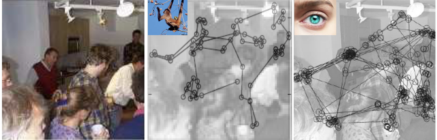
Figure 11: Monkey or human: can you tell the difference? The center image has been obtained by superimposing a typical trajectory of spider monkeys foraging in the forest of the Mexican Yucatan, as derived from [Ramos-Fernandez et al. (2004)], on the “party picture” (left image) used in [Brockmann and Geisel (2000)]. The right image is an actual human scan path (modified after brockgeis)

The fact that the physics underlying foraging overlaps with that of several other kinds of complex random searches and stochastic optimization problems [Viswanathan et al. (2011)], and notably with that of visual exploration via gaze shifts [Viswanathan et al. (2011), Marlow et al. (2015), Brockmann and Geisel (2000)], makes available a variety of analytical tools beyond classic metrics exploited in computer vision or psychology. For instance, in Figure 12, it is shown how the gaze shift amplitude modes from human observers can be compared with those generated via simulation by using the complementary Cumulative Distribution Function (CCDF), which provides a precise description of the distribution of the gaze shift by considering its upper tail behavior. This can be defined as $\overline{F}(x)=P(|\mathbf{r}|>x)=1-F(x)$, where $F$ is the cumulative distribution function (CDF) of amplitudes. Consideration of the upper tail, i.e. the CCDF of jump lengths is a standard convention in foraging, human mobility, and anomalous diffusion research [Viswanathan et al. (2011)].

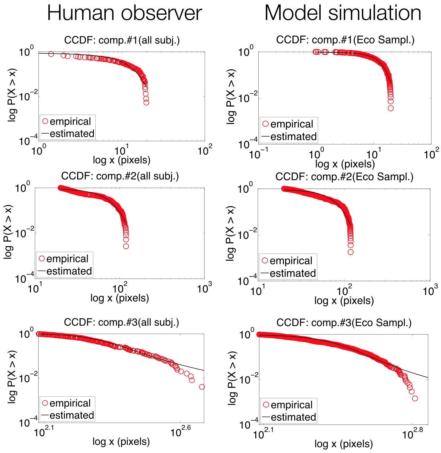
Figure 12: Analysis of gaze shift dynamics from the monica03 video. The left column shows the double log plot of the CCDF obtained from the gaze magnitude distribution of all subjects: i) the smooth-pursuit mode (top row); ii) the small saccade mode (middle); iii) large saccades (bottom). The right column presents the equivalent CCDFs obtained via model simulation.

To sum up, foraging offers a novel perspective for formulating models and related evaluations of visual attention and oculomotor behavior [Wolfe (2013)]. Unifying hypotheses such as the oculomotor continuum from exploration to fixation by otero2013oculomotor can be reconsidered in the light of fundamental theorems of statistical mechanics [Weron and Magdziarz (2010)].

Relationship between Attentive vision and Foraging Video stream attentive processing Patchy landscape foraging Observer Forager Observer’s gaze shift Forager’s relocation Region of interest Patch Proto-object Candidate prey Detected object Prey Region selection Patch choice Deploying attention to object Prey choice and handling Disengaging from object Prey leave Region leave Patch leave or giving-up

Interestingly enough, the reformulation of visual attention in terms of foraging theory is not simply an informing metaphor. It has been argued that what was once foraging for tangible resources in a physical space became, over evolutionary time, foraging in cognitive space for information related to those resources [Hills (2006)], and such adaptations play a fundamental role in goal-directed deployment of visual attention [Wolfe (2013)].

5 Bringing value into the game: a doorway to affective modulation

The introduction of a goal level, either exogenous (originating from outside the observer’s organism) or endogenous (internal) is not an innocent shift.

From a classical cognitive perspective, the assignment of a task to the observer implicitly defines a value for every point of the space, in the sense that information in some points is more relevant than in others for the completion of the task; the shifting of the gaze on a particular point, in turn, determines the payoff that can be gained.

There is a number of psychological and neurobiological studies showing the availability of value maps and loci of reward influencing the final gaze shift [Platt and Glimcher (1999), Leon and Shadlen (1999), Ikeda and Hikosaka (2003), Hikosaka et al. (2006)]. The payoff is nothing else that the value, with respect to the completion of the task, obtained by moving the fovea in a given position. Thus points associated with high values produce, when fixated, high payoffs since these fixations bring the observer closer to her/his goal. For instance, in [Clavelli et al. (2014)] and in [Napoletano et al. (2015)], reward was introduced to make a choice among the candidate gaze shifts stochastically sampled according to Eq. 12, in terms of expected reward (e.g., tuned by the probability of finding the task-assigned object).

Figure 13 presents one example of the different scan paths obtained by progressively reducing the levels of representation in the perceptual evaluation component presented in Figure 8 [Clavelli et al. (2014), Napoletano et al. (2015)].

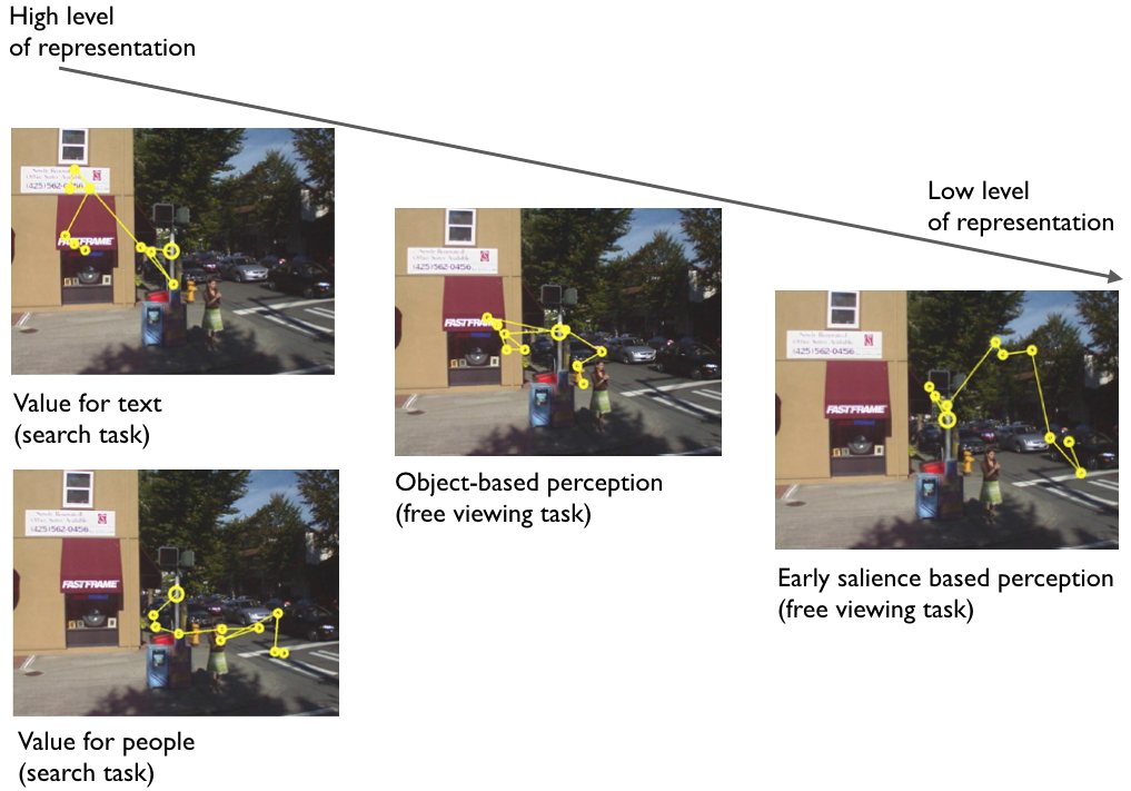
Figure 13: Different scan paths originated from the progressive reduction of representation levels in the perceptual evaluation component presented in Figure 8.

Value set by the given goal can weight differently the objects within the scene, thus purposively biasing the scan path. Gaze is still uniformly deployed to relevant items within the scene (people, text) when object-based representation is exploited. When salience alone is used, the generated scan path fails in accounting for the relevant items and bears no relation with the semantics which can be attributed to the scene.

The use of value and reward endow attentive models with the capability of handling complex task. For instance, BocCOGN2014 considered the goal of text spotting in unconstrained urban environments, and its validation encompassed data gathered from a mobile eye tracking device [Clavelli (2014)]. napboc_TIP2015 extended the foraging framework to cope with the difficult problem of attentive monitoring of multiple video streams in a videosurveillance setting.

Yet, developing eye guidance models based on reward is a difficult endeavour and computational models that use reward and uncertainty as central components are still in their infancy (but see the discussion by TatlerBallard2011eye). In this respect the remarkable work by Ballard and collegues counters the stream. Whilst salience, proto-objects and objects are representations that have been largely addressed in the context of human eye movements, albeit with different emphasis, in contrast, value has been neglected until recently [Schütz et al. (2011)]. One reason is that in the real world there is seldom direct payoff (no orange juice for a primary reward) for making good eye movements or punishment for bad ones.

However, the high attentional priority of ecologically pertinent stimuli can also be explained by mechanisms that do not implicate learning value through repeated pairings with reward. For example, a bias to attend to socially relevant stimuli is evident from infancy [Anderson (2013)]. More generally, the selection of stimuli by attention has important implications for the survival and wellbeing of an organism, and attentional priority reflects the overall value of such selection (see anderson2013value for a discussion). Indeed, engaging attention with potentially harmful and beneficial stimuli guarantees that the relevant ones are selected early so to gauge the exact nature of the potential threat or opportunity and to readily initiate defensive or approach behavior.

Under these circumstances, maunsell2004neuronal has proposed a broad definition of reward, which includes “not only the immediate primary rewards, but also other factors: the preference for a novel location or stimulus, the satisfaction of performing well or the desire to complete a given task.” Such definition is consistent with the different psychological facets of reward [Berridge and Robinson (2003)]: i) learning (including explicit and implicit knowledge produced by associative conditioning and cognitive processes); ii) affect or emotion (implicit “liking” and conscious pleasure); iii) motivation (implicit incentive salience “wanting” and cognitive incentive goals). Thus, value representation level is central to both goal-driven affective and cognitive engagement with stimuli in the outside world.

In this broader perspective, the effort to put value and reward into the game shows his inner worth in that, by accounting for the many aspects of “biological value” - salience, significance, unpredictability, affective content - , it paves the way to a wider dimension of information processing, as most recent results on the affective modulation of the visual processing stream advocate [Pessoa (2008), Pessoa and Adolphs (2010)], and to the effective exploitation of computational attention models in the emerging domain of social signal processing [Vinciarelli et al. (2009)].

A number of important studies in the psychological literature (see, for a discussion, calvo2006eye,Humphrey_lamb) have addressed the relationship between overt attention behavior and emotional content of pictures. Many of them investigate specific issues related to individuals such as trait anxiety, social anxiety, spider phobia, and exploit restricted sets of stimuli such as emotional faces or spiders. In turn, the study by calvo2006eye has exploited natural images and normal subjects, demonstrating an emotional bias both in attentional orienting and engagement among normal participants and using a wider range of emotional pictures. Results might be summarised as follows: i) emotionally pleasant and unpleasant pictures capture attention more readily than neutral pictures; ii) the emotional bias can be observed early in initial orienting and subsequent engagement of attention; iii) the early stimulus-driven attentional capture by emotional stimuli can be counteracted by goal-driven control in later stages of picture processing.

Peculiarly relevant to our case, Humphrey_lamb have shown that visual saliency does influence eye movements, but the effect is reliably reduced when an emotional object is present. Pictures containing negative objects were recognized more accurately and recalled in greater detail, and participants fixated more on negative objects than positive or neutral ones. Initial fixations were more likely to be on emotional objects than more visually salient neutral ones. Consistently with calvo2006eye, the overall result suggest that the processing of emotional features occurs at a very early stage of perception.

As a matter of fact, emotional factors are completely neglected in the realm of computational models of attention and gaze shifts. Some efforts have been spent in the field of social robotics, where motivational drives have an indirect influence on attention by influencing the behavioral context, which, in turn, is used to directly manipulate the gains of the attention system (e.g. by tuning the gains of different bottom-up saliency map, breazeal2001active). Yet, beyond these broadly related attempts, taking into account the specific influence of affect on eye-behaviour is not a central concern within this field (for a wide review, see ferreira2014attentional). Recent works in the image processing and pattern recognition community use eye tracking data for the inverse problem of the recognition of emotional content of images (e.g.,tavakoli2014emotional,Tavakoli_PONE2015) or implicit tagging of videos [Soleymani et al. (2012)]. Thus, they do not address the generative problem of how emotional factors contribute to the generation of gaze shifts in visual tasks.

By contrast, neuroscience has shown that, crucially, cognitive and emotional contributions cannot be separated, as outlined in Figure 14.

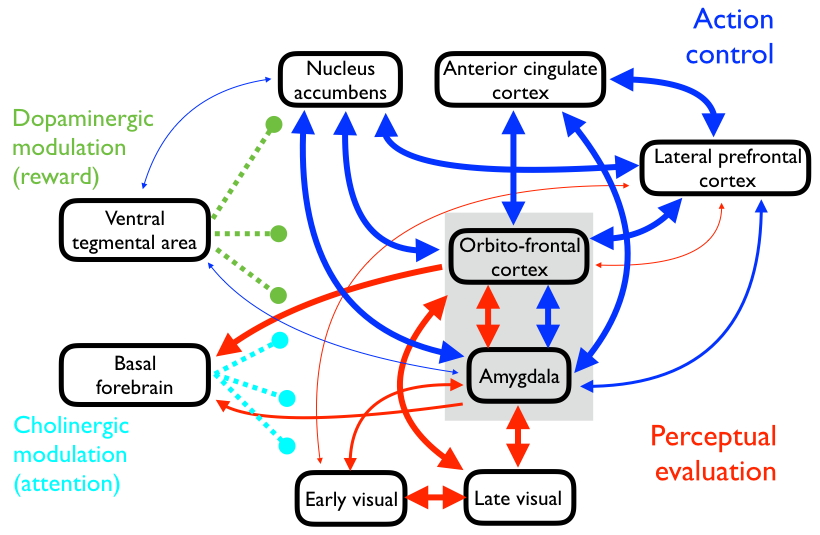
Figure 14: Circuits for the processing of visual information and for the executive control [Pessoa (2008)] show that action and perception components are inextricably linked through the mediation of the amygdala and the posterior orbitofrontal cortex (OFC). These structures are considered to be the neural substrate of emotional valence and arousal [Salzman and Fusi (2010)]. The ventral tegmental area (vTA) and the basal forebrain are responsible for diffuse neuromodulatory effects related to reward and attention. Anterior cingulate cortex (ACC) is likely to be involved in conflict detection and/or error monitoring but also in in computing the benefits and costs of acting by encoding the probability of reward. Nucleus accumbens is usually related to motivation.The lateral prefrontal cortex (LPFC) plays a central role at the cognitive level in maintaining and manipulating information, but also integrates this content with both affective and motivational information. Line thickness depicts approximate connection strength

The scheme presented, which summarises an ongoing debate [Pessoa (2008)], shows that responses from early and late visual cortex reflecting stimulus significance will be a result of simultaneous top-down modulation from fronto-parietal attentional regions (LPFC) and emotional modulation from the amygdala [Mohanty and Sussman (2013)]. On the one hand, stimulus’ affective value appears to drive attention and enhance the processing of emotionally modulated information. On the other hand, exogenously driven attention influences the outcome of affectively significant stimuli [Pessoa (2008)]. As a prominent result, the cognitive or affective origin of the modulation is lost and stimulus’ effect on behaviour is both cognitive and emotional. At the same time, the cognitive control system (LPFC, ACC) guides behaviour while maintaining and manipulating goal-related information; however strategies for action dynamically incorporate value through the mediation of the nucleus accumbens, the amygdala, and the OFC. Eventually, basal forebrain cholinergic neurons provide regulation of arousal and attention [Goard and Dan (2009)], while dopamine neurons located in the vTA modulate the prediction and expectation of future rewards [Pessoa (2008)].

It is to be noted in Figure 14 the central role of the amygdala and the OFC. It has been argued [Salzman and Fusi (2010)] that their tight interaction provides a suitable ground for representing, at the psychological level the core affect dimensions [Russell (2003)] of valence (pleasure–displeasure conveyed by the visual stimuli) and arousal (activation–deactivation). From a computational standpoint, the observer’s core affect can in principle be modelled as a dynamic latent space [Vitale et al. (2014)], which we surmise might be readily embedded within the loop as proposed in Fig. 15. This way, gaze shifts would benefit from the crucial emotional mediation between the action control and perceptual evaluation components.

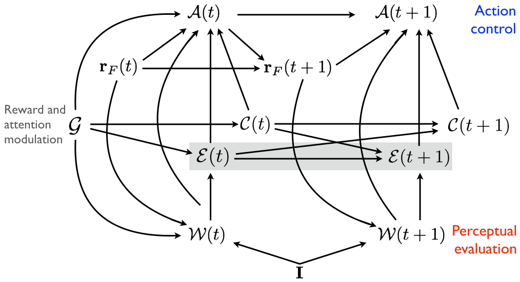
Figure 15: The perception-action loop unfolded in time as a dynamic PGM as in Figure 9, but integrated with the core affect latent dimension abstracted as the RV $\mathcal{E}(t)$. $\mathcal{C}(t)$ stands for a higher cognitive control RV. To simplify the graphics, conditional dependencies $\mathcal{G}\rightarrow\mathcal{A}(t+1)$ and $\mathcal{G}\rightarrow\mathcal{W}(t+1)$ have been omitted.

6 Conclusion

Time is ripe to abandon the marshland of mass production and evaluation of bottom-up saliency techniques. Such boundless effort is partially based on a fatally flawed assumption [Santini and Dumitrescu (2008)]: that visual data have a meaning per se, which can be derived as a function of a certain representation of the data themselves. Meaning is an outcome of an interpretative process rather than a property of the viewed scene. It is the act of perceiving, contextual and situated, that gives a scene its meaning [Wittgenstein (2010)].

The course of modelling can be more fruitfully directed not only to climb the hierarchy of representation levels and to cope with overlooked aspects of eye guidance, but to eventually reappraise the observer within his natural setting: an active observer compelled to purposively exploit visual attention for accomplishing real-world tasks [Merleau–Ponty (1945)].

References

- [1]
- Aloimonos et al. (1988) John Aloimonos, Isaac Weiss, and Amit Bandyopadhyay. 1988. Active vision. International journal of computer vision 1, 4 (1988), 333–356.
- Anderson (2013) Brian A Anderson. 2013. A value-driven mechanism of attentional selection. Journal of vision 13, 3 (2013).
- Bajcsy and Campos (1992) Ruzena Bajcsy and Mario Campos. 1992. Active and exploratory perception. CVGIP: Image Understanding 56, 1 (1992), 31–40.
- Baldi and Itti (2010) P. Baldi and L. Itti. 2010. Of bits and wows: A Bayesian theory of surprise with applications to attention. Neural Networks 23, 5 (2010), 649–666.
- Ballard (1991) D.H. Ballard. 1991. Animate vision. Artificial intelligence 48, 1 (1991), 57–86.
- Bartumeus and Catalan (2009) F. Bartumeus and J. Catalan. 2009. Optimal search behavior and classic foraging theory. Journal of Physics A: Mathematical and Theoretical 42 (2009), 434002.
- Begum et al. (2010) M. Begum, F. Karray, G.K.I. Mann, and R.G. Gosine. 2010. A probabilistic model of overt visual attention for cognitive robots. Systems, Man, and Cybernetics, Part B: Cybernetics, IEEE Transactions on 40, 5 (2010), 1305–1318.
- Berridge and Robinson (2003) Kent C Berridge and Terry E Robinson. 2003. Parsing reward. Trends in neurosciences 26, 9 (2003), 507–513.
- Boccignone (2008) G. Boccignone. 2008. Nonparametric Bayesian attentive video analysis. In Proc. 19th International Conference on Pattern Recognition, ICPR 2008. IEEE Press, 1–4.
- Boccignone and Ferraro (2004) G. Boccignone and M. Ferraro. 2004. Modelling gaze shift as a constrained random walk. Physica A: Statistical Mechanics and its Applications 331, 1-2 (2004), 207–218.
- Boccignone and Ferraro (2013) Giuseppe Boccignone and Mario Ferraro. 2013. Feed and fly control of visual scanpaths for foveation image processing. annals of telecommunications-annales des télécommunications 68, 3-4 (2013), 201–217.
- Boccignone and Ferraro (2014) Giuseppe Boccignone and Mario Ferraro. 2014. Ecological Sampling of Gaze Shifts. IEEE Trans. on Cybernetics 44, 2 (Feb 2014), 266–279.
- Boccignone et al. (2008) G. Boccignone, A. Marcelli, P. Napoletano, G. Di Fiore, G. Iacovoni, and S. Morsa. 2008. Bayesian integration of face and low-level cues for foveated video coding. IEEE Transactions on Circuits and Systems for Video Technology 18, 12 (2008), 1727–1740.
- Borji et al. (2014) Ali Borji, Ming-Ming Cheng, Huaizu Jiang, and Jia Li. 2014. Salient object detection: A survey. arXiv preprint arXiv:1411.5878 (2014).
- Borji and Itti (2013) A. Borji and L. Itti. 2013. State-of-the-Art in Visual Attention Modeling. IEEE Transactions on Pattern Analysis and Machine Intelligence 35, 1 (2013), 185–207.
- Borji et al. (2012) Ali Borji, Dicky N Sihite, and Laurent Itti. 2012. An Object-Based Bayesian Framework for Top-Down Visual Attention. In Twenty-Sixth AAAI Conference on Artificial Intelligence.
- Breazeal et al. (2001) Cynthia Breazeal, Aaron Edsinger, Paul Fitzpatrick, and Brian Scassellati. 2001. Active vision for sociable robots. IEEE Transactions on Systems, Man and Cybernetics, Part A: Systems and Humans 31, 5 (2001), 443–453.
- Brockmann and Geisel (2000) D. Brockmann and T. Geisel. 2000. The ecology of gaze shifts. Neurocomputing 32, 1 (2000), 643–650.
- Bruce and Tsotsos (2009) Neil DB Bruce and John K Tsotsos. 2009. Saliency, attention, and visual search: An information theoretic approach. Journal of vision 9, 3 (2009), 5–5.
- Bruce et al. (2015) Neil DB Bruce, Calden Wloka, Nick Frosst, Shafin Rahman, and John K Tsotsos. 2015. On computational modeling of visual saliency: Examining what’s right, and what’s left. Vision research 116 (2015), 95–112.
- Bylinskii et al. (2015) Z Bylinskii, EM DeGennaro, R Rajalingham, H Ruda, J Zhang, and JK Tsotsos. 2015. Towards the quantitative evaluation of visual attention models. Vision research 116 (2015), 258–268.
- Cain et al. (2012) Matthew S Cain, Edward Vul, Kait Clark, and Stephen R Mitroff. 2012. A Bayesian optimal foraging model of human visual search. Psychological science 23, 9 (2012), 1047–1054.
- Canosa (2009) R.L. Canosa. 2009. Real-world vision: Selective perception and task. ACM Transactions on Applied Perception 6, 2 (2009), 11.
- Cerf et al. (2009) M. Cerf, E.P. Frady, and C. Koch. 2009. Faces and text attract gaze independent of the task: Experimental data and computer model. Journal of Vision 9, 12 (2009).
- Cerf et al. (2008) M. Cerf, J. Harel, W. Einhäuser, and C. Koch. 2008. Predicting human gaze using low-level saliency combined with face detection. Advances in neural information processing systems 20 (2008).
- Chernyak and Stark (2001) D. A. Chernyak and L. W. Stark. 2001. Top–Down Guided Eye Movements. IEEE Trans. Systems Man Cybernetics - B 31 (2001), 514–522.
- Chikkerur et al. (2010) S. Chikkerur, T. Serre, C. Tan, and T. Poggio. 2010. What and where: A Bayesian inference theory of attention. Vision research 50, 22 (2010), 2233–2247.
- Clavelli (2014) Antonio Clavelli. 2014. A computational model of eye guidance, searching for text in real scene images. Ph.D. Dissertation. Universitat Autónoma de Barcelona. Departament de Ciéncies de la Computació. http://ddd.uab.cat/record/127173
- Clavelli et al. (2014) Antonio Clavelli, Dimosthenis Karatzas, Josep Lladós, Mario Ferraro, and Giuseppe Boccignone. 2014. Modelling Task-Dependent Eye Guidance to Objects in Pictures. Cognitive Computation 6, 3 (2014), 558–584.
- Coen-Cagli et al. (2008) Ruben Coen-Cagli, Paolo Coraggio, Paolo Napoletano, and Giuseppe Boccignone. 2008. What the draughtsman’s hand tells the draughtsman’s eye: A sensorimotor account of drawing. International Journal of Pattern Recognition and Artificial Intelligence 22, 05 (2008), 1015–1029.
- Coen-Cagli et al. (2009) Ruben Coen-Cagli, Paolo Coraggio, Paolo Napoletano, Odelia Schwartz, Mario Ferraro, and Giuseppe Boccignone. 2009. Visuomotor characterization of eye movements in a drawing task. Vision research 49, 8 (2009), 810–818.
- Cordeschi (2002) Roberto Cordeschi. 2002. The discovery of the artificial: Behavior, mind and machines before and beyond cybernetics. Vol. 28. Springer Science & Business Media.
- deCroon et al. (2011) G.C.H.E. deCroon, E.O. Postma, and H. J. van den Herik. 2011. Adaptive Gaze Control for Object Detection. Cognitive Computation 3 (2011), 264–278.
- Dorr et al. (2010) M. Dorr, T. Martinetz, K.R. Gegenfurtner, and E. Barth. 2010. Variability of eye movements when viewing dynamic natural scenes. Journal of Vision 10, 10 (2010).
- Einhäuser et al. (2008) Wolfgang Einhäuser, Merrielle Spain, and Pietro Perona. 2008. Objects predict fixations better than early saliency. Journal of Vision 8, 14 (2008). DOI:http://dx.doi.org/10.1167/8.14.18
- Elazary and Itti (2010) Lior Elazary and Laurent Itti. 2010. A Bayesian model for efficient visual search and recognition. Vision research 50, 14 (2010), 1338–1352.
- Ellis and Stark (1986) S.R. Ellis and L. Stark. 1986. Statistical dependency in visual scanning. Human Factors: The Journal of the Human Factors and Ergonomics Society 28, 4 (1986), 421–438.
- Feldman and Friston (2010) Harriet Feldman and Karl Friston. 2010. Attention, uncertainty, and free-energy. Frontiers in human neuroscience 4 (2010), 215.
- Feng (2006) G. Feng. 2006. Eye movements as time-series random variables: A stochastic model of eye movement control in reading. Cognitive Systems Research 7, 1 (2006), 70–95.
- Ferreira and Dias (2014) Joao Filipe Ferreira and Joana Dias. 2014. Attentional Mechanisms for Socially Interactive Robots–A Survey. IEEE Transactions on Autonomous Mental Development 6, 2 (2014), 110–125.
- Foulsham and Underwood (2008) Tom Foulsham and Geoffrey Underwood. 2008. What can saliency models predict about eye movements? Spatial and sequential aspects of fixations during encoding and recognition. Journal of Vision 8, 2 (2008).
- Friston (2010) Karl Friston. 2010. The free-energy principle: a unified brain theory? Nature Reviews Neuroscience 11, 2 (2010), 127–138.
- Friston et al. (2013) Karl Friston, Philipp Schwartenbeck, Thomas Fitzgerald, Michael Moutoussis, Tim Behrens, and Raymond J Dolan. 2013. The anatomy of choice: active inference and agency. Frontiers in Human Neuroscience 7 (2013), 598.
- Goard and Dan (2009) Michael Goard and Yang Dan. 2009. Basal forebrain activation enhances cortical coding of natural scenes. Nature neuroscience 12, 11 (2009), 1444–1449.
- Hacisalihzade et al. (1992) S.S. Hacisalihzade, L.W. Stark, and J.S. Allen. 1992. Visual perception and sequences of eye movement fixations: A stochastic modeling approach. IEEE Trans. Syst., Man, Cybern. 22, 3 (1992), 474–481.
- Harel et al. (2007) J. Harel, C. Koch, and P. Perona. 2007. Graph-based visual saliency. In Advances in neural information processing systems, Vol. 19. MIT Press, Cambridge, MA, 545–552.
- Hikosaka et al. (2006) Okihide Hikosaka, Kae Nakamura, and Hiroyuki Nakahara. 2006. Basal Ganglia Orient Eyes to Reward. Journal of Neurophysiology 95, 2 (2006), 567–584.
- Hills (2006) Thomas T Hills. 2006. Animal Foraging and the Evolution of Goal-Directed Cognition. Cognitive Science 30, 1 (2006), 3–41.
- Humphrey et al. (2012) Katherine Humphrey, Geoffrey Underwood, and Tony Lambert. 2012. Salience of the lambs: A test of the saliency map hypothesis with pictures of emotive objects. Journal of Vision 12, 1 (2012), 22. DOI:http://dx.doi.org/10.1167/12.1.22
- Ikeda and Hikosaka (2003) Takuro Ikeda and Okihide Hikosaka. 2003. Reward-dependent gain and bias of visual responses in primate superior colliculus. Neuron 39, 4 (2003), 693–700.
- Itti and Baldi (2009) L. Itti and P. Baldi. 2009. Bayesian surprise attracts human attention. Vision research 49, 10 (2009), 1295–1306.
- Itti et al. (1998) L. Itti, C. Koch, and E. Niebur. 1998. A Model of Saliency-based Visual Attention for Rapid Scene Analysis. IEEE Transactions on Pattern Analysis and Machine Intelligence 20 (1998), 1254–1259.
- Jiang et al. (2015) Lai Jiang, Mai Xu, Zhaoting Ye, and Zulin Wang. 2015. Image Saliency Detection With Sparse Representation of Learnt Texture Atoms. In Proceedings of the IEEE International Conference on Computer Vision Workshops. 54–62.
- Judd et al. (2009) Tilke Judd, Krista Ehinger, Frédo Durand, and Antonio Torralba. 2009. Learning to predict where humans look. In IEEE 12th International conference on Computer Vision. IEEE, 2106–2113.
- Keech and Resca (2010) TD Keech and L. Resca. 2010. Eye movements in active visual search: A computable phenomenological model. Attention, Perception, & Psychophysics 72, 2 (2010), 285–307.
- Kienzle et al. (2009) Wolf Kienzle, Matthias O Franz, Bernhard Schölkopf, and Felix A Wichmann. 2009. Center-surround patterns emerge as optimal predictors for human saccade targets. Journal of vision 9, 5 (2009), 7–7.
- Kienzle et al. (2006) Wolf Kienzle, Felix A Wichmann, Matthias O Franz, and Bernhard Schölkopf. 2006. A nonparametric approach to bottom-up visual saliency. In Advances in neural information processing systems. 689–696.
- Kimura et al. (2008) A. Kimura, D. Pang, T. Takeuchi, J. Yamato, and K. Kashino. 2008. Dynamic Markov random fields for stochastic modeling of visual attention. In Proc. ICPR ’08. IEEE, 1–5.
- Kowler (2011) E. Kowler. 2011. Eye movements: The past 25 years. Vision Research 51, 13 (2011), 1457–1483. 50th Anniversary Special Issue of Vision Research - Volume 2.
- Krizhevsky et al. (2012) Alex Krizhevsky, Ilya Sutskever, and Geoffrey E. Hinton. 2012. ImageNet Classification with Deep Convolutional Neural Networks. In Advances in Neural Information Processing Systems 25, F. Pereira, C. J. C. Burges, L. Bottou, and K. Q. Weinberger (Eds.). Curran Associates, Inc., 1097–1105. http://papers.nips.cc/paper/4824-imagenet-classification-with-deep-convolutional-neural-networks.pdf
- Kruthiventi et al. (2015) Srinivas SS Kruthiventi, Kumar Ayush, and R Venkatesh Babu. 2015. DeepFix: A Fully Convolutional Neural Network for predicting Human Eye Fixations. arXiv preprint arXiv:1510.02927 (2015).
- Kümmerer et al. (2014) Matthias Kümmerer, Lucas Theis, and Matthias Bethge. 2014. Deep Gaze I: Boosting saliency prediction with feature maps trained on ImageNet. arXiv preprint arXiv:1411.1045 (2014).
- Kümmerer et al. (2015) Matthias Kümmerer, Thomas SA Wallis, and Matthias Bethge. 2015. Information-theoretic model comparison unifies saliency metrics. Proceedings of the National Academy of Sciences 112, 52 (2015), 16054–16059.
- Lang et al. (2012) Congyan Lang, Guangcan Liu, Jian Yu, and Shuicheng Yan. 2012. Saliency detection by multitask sparsity pursuit. IEEE Transactions on Image Processing 21, 3 (2012), 1327–1338.
- Le Meur and Coutrot (2016) Olivier Le Meur and Antoine Coutrot. 2016. Introducing context-dependent and spatially-variant viewing biases in saccadic models. Vision Research 121 (2016), 72–84.
- Le Meur and Liu (2015) Olivier Le Meur and Zhi Liu. 2015. Saccadic model of eye movements for free-viewing condition. Vision research 116 (2015), 152–164.
- LeCun et al. (2015) Yann LeCun, Yoshua Bengio, and Geoffrey Hinton. 2015. Deep learning. Nature 521, 7553 (2015), 436–444.
- Leon and Shadlen (1999) Matthew I Leon and Michael N Shadlen. 1999. Effect of expected reward magnitude on the response of neurons in the dorsolateral prefrontal cortex of the macaque. Neuron 24, 2 (1999), 415–425.
- Lin et al. (2014) Yuetan Lin, Shu Kong, Donghui Wang, and Yueting Zhuang. 2014. Saliency detection within a deep convolutional architecture. In Workshops at the Twenty-Eighth AAAI Conference on Artificial Intelligence.
- MacKay (2002) D.J.C. MacKay. 2002. Information Theory, Inference and Learning Algorithms. Cambridge University Press, Cambridge, UK.
- Marat et al. (2013) Sophie Marat, Anis Rahman, Denis Pellerin, Nathalie Guyader, and Dominique Houzet. 2013. Improving Visual Saliency by Adding Face Feature Map and Center Bias . Cognitive Computation 5, 1 (2013), 63–75.
- Marlow et al. (2015) Colleen A Marlow, Indre V Viskontas, Alisa Matlin, Cooper Boydston, Adam Boxer, and Richard P Taylor. 2015. Temporal Structure of Human Gaze Dynamics Is Invariant During Free Viewing. PloS one 10, 9 (2015), e0139379.
- Marr (1982) D. Marr. 1982. Vision: A Computational Investigation into the Human Representation and Processing of Visual Information. W.H. Freeman, New York.
- Martinez et al. (2008) H. Martinez, M. Lungarella, and R. Pfeifer. 2008. Stochastic Extension to the Attention-Selection System for the iCub. University of Zurich, Tech. Rep (2008).
- Mathe and Sminchisescu (2015) Stefan Mathe and Cristian Sminchisescu. 2015. Actions in the eye: dynamic gaze datasets and learnt saliency models for visual recognition. Pattern Analysis and Machine Intelligence, IEEE Transactions on 37, 7 (2015), 1408–1424.
- Maunsell (2004) John HR Maunsell. 2004. Neuronal representations of cognitive state: reward or attention? Trends in cognitive sciences 8, 6 (2004), 261–265.
- Merleau–Ponty (1945) Maurice Merleau–Ponty. 1945. Phénoménologie de la perception. Gallimard, Paris.
- Mohanty and Sussman (2013) Aprajita Mohanty and Tamara J Sussman. 2013. Top-down modulation of attention by emotion. Frontiers in Human Neuroscience 7, 102 (2013). http://www.frontiersin.org/human_neuroscience/10.3389/fnhum.2013.00102/full
- Murphy (2012) Kevin P Murphy. 2012. Machine learning: a probabilistic perspective. MIT press, Cambridge, MA.
- Nagai (2009a) Y. Nagai. 2009a. From bottom-up visual attention to robot action learning. In Proceedings of 8 IEEE International Conference on Development and Learning. IEEE Press.
- Nagai (2009b) Y. Nagai. 2009b. Stability and sensitivity of bottom-up visual attention for dynamic scene analysis. In Proceedings of the 2009 IEEE/RSJ international conference on Intelligent robots and systems. IEEE Press, 5198–5203.
- Najemnik and Geisler (2005) J. Najemnik and W.S. Geisler. 2005. Optimal eye movement strategies in visual search. Nature 434, 7031 (2005), 387–391.
- Napoletano et al. (2015) P. Napoletano, G. Boccignone, and F. Tisato. 2015. Attentive monitoring of multiple video streams driven by a Bayesian foraging strategy. IEEE Trans. on Image Processing 24, 11 (Nov. 2015), 3266 – 3281.
- Nummenmaa et al. (2006) Lauri Nummenmaa, Jukka Hyönä, and Manuel G Calvo. 2006. Eye movement assessment of selective attentional capture by emotional pictures. Emotion 6, 2 (2006), 257.
- Otero-Millan et al. (2013) Jorge Otero-Millan, Stephen L Macknik, Rachel E Langston, and Susana Martinez-Conde. 2013. An oculomotor continuum from exploration to fixation. Proceedings of the National Academy of Sciences 110, 15 (2013), 6175–6180.
- Over et al. (2007) E.A.B. Over, I.T.C. Hooge, B.N.S. Vlaskamp, and C.J. Erkelens. 2007. Coarse-to-fine eye movement strategy in visual search. Vision Research 47 (2007), 2272–2280.
- Pessoa (2008) Luiz Pessoa. 2008. On the relationship between emotion and cognition. Nature Reviews Neuroscience 9, 2 (2008), 148–158.
- Pessoa and Adolphs (2010) Luiz Pessoa and Ralph Adolphs. 2010. Emotion processing and the amygdala: from a’low road’to’many roads’ of evaluating biological significance. Nature Reviews Neuroscience 11, 11 (2010), 773–783.
- Platt and Glimcher (1999) Michael L Platt and Paul W Glimcher. 1999. Neural correlates of decision variables in parietal cortex. Nature 400, 6741 (1999), 233–238.
- Privitera (2006) Claudio M Privitera. 2006. The scanpath theory: its definitions and later developments. In Electronic Imaging 2006. International Society for Optics and Photonics, 60570A–60570A.
- R.-Tavakoli et al. (2015) Hamed R.-Tavakoli, Adham Atyabi, Antti Rantanen, Seppo J. Laukka, Samia Nefti-Meziani, and Janne Heikkil? 2015. Predicting the Valence of a Scene from Observers? Eye Movements. PLoS ONE 10, 9 (09 2015), 1–19. DOI:http://dx.doi.org/10.1371/journal.pone.0138198
- Ramos-Fernandez et al. (2004) G. Ramos-Fernandez, J.L. Mateos, O. Miramontes, G. Cocho, H. Larralde, and B. Ayala-Orozco. 2004. Lévy walk patterns in the foraging movements of spider monkeys (Ateles geoffroyi). Behavioral Ecology and Sociobiology 55, 3 (2004), 223–230.
- Rao (2005) R.P.N. Rao. 2005. Bayesian inference and attentional modulation in the visual cortex. Neuroreport 16, 16 (2005), 1843.
- Rao et al. (2002) Rajesh P.N. Rao, Gregory J. Zelinsky, Mary M. Hayhoe, and Dana H. Ballard. 2002. Eye movements in iconic visual search. Vision Research 42, 11 (2002), 1447 – 1463.
- Rensink (2000) R.A. Rensink. 2000. The dynamic representation of scenes. Visual Cognition 1, 3 (2000), 17–42.
- Rothenstein and Tsotsos (2008) Albert L Rothenstein and John K Tsotsos. 2008. Attention links sensing to recognition. Image and Vision Computing 26, 1 (2008), 114–126.
- Rothkopf et al. (2007) C.A. Rothkopf, D.H. Ballard, and M.M. Hayhoe. 2007. Task and context determine where you look. Journal of Vision 7, 14 (2007).
- Russell (2003) James A Russell. 2003. Core affect and the psychological construction of emotion. Psychological review 110, 1 (2003), 145.
- Rutishauser and Koch (2007) U. Rutishauser and C. Koch. 2007. Probabilistic modeling of eye movement data during conjunction search via feature-based attention. Journal of Vision 7, 6 (2007).
- Salzman and Fusi (2010) C Daniel Salzman and Stefano Fusi. 2010. Emotion, cognition, and mental state representation in amygdala and prefrontal cortex. Annual review of neuroscience 33 (2010), 173.
- Santini and Dumitrescu (2008) Simone Santini and Alexandra Dumitrescu. 2008. Context as a non-ontological determinant of semantics. In Semantic Multimedia. Springer, 121–136.
- Schütz et al. (2011) A.C. Schütz, D.I. Braun, and K.R. Gegenfurtner. 2011. Eye movements and perception: A selective review. Journal of Vision 11, 5 (2011).
- Seo and Milanfar (2009) HJ Seo and P. Milanfar. 2009. Static and space-time visual saliency detection by self-resemblance. Journal of Vision 9, 12 (2009), 1–27.
- Shen and Zhao (2014) Chengyao Shen and Qi Zhao. 2014. Learning to predict eye fixations for semantic contents using multi-layer sparse network. Neurocomputing 138 (2014), 61–68.
- Soleymani et al. (2012) Mohammad Soleymani, Jeroen Lichtenauer, Thierry Pun, and Maja Pantic. 2012. A multimodal database for affect recognition and implicit tagging. Affective Computing, IEEE Transactions on 3, 1 (2012), 42–55.
- Srinivas et al. (2016) Suraj Srinivas, Ravi Kiran Sarvadevabhatla, Konda Reddy Mopuri, Nikita Prabhu, Srinivas Kruthiventi, and Venkatesh Babu Radhakrishnan. 2016. A taxonomy of Deep Convolutional Neural Nets for Computer Vision. Frontiers in Robotics and AI 2, 36 (2016). DOI:http://dx.doi.org/10.3389/frobt.2015.00036
- Strasburger et al. (2011) Hans Strasburger, Ingo Rentschler, and Martin Jüttner. 2011. Peripheral vision and pattern recognition: A review. Journal of Vision 11, 5 (2011).
- Sun et al. (2008) Yaoru Sun, Robert Fisher, Fang Wang, and Herman Martins Gomes. 2008. A computer vision model for visual-object-based attention and eye movements. Computer Vision and Image Understanding 112, 2 (2008), 126 – 142.
- Tatler et al. (2011) B.W. Tatler, M.M. Hayhoe, M.F. Land, and D.H. Ballard. 2011. Eye guidance in natural vision: Reinterpreting salience. Journal of vision 11, 5 (2011).
- Tatler and Vincent (2008) B.W. Tatler and B.T. Vincent. 2008. Systematic tendencies in scene viewing. Journal of Eye Movement Research 2, 2 (2008), 1–18.
- Tatler and Vincent (2009) B.W. Tatler and B.T. Vincent. 2009. The prominence of behavioural biases in eye guidance. Visual Cognition 17, 6-7 (2009), 1029–1054.
- Tavakoli et al. (2013) Hamed Rezazadegan Tavakoli, Esa Rahtu, and Janne Heikkilä. 2013. Stochastic bottom–up fixation prediction and saccade generation. Image and Vision Computing 31, 9 (2013), 686–693.
- Tavakoli et al. (2014) Hamed R Tavakoli, Victoria Yanulevskaya, Esa Rahtu, Janne Heikkila, and Nicu Sebe. 2014. Emotional Valence Recognition, Analysis of Salience and Eye Movements. In 2014 22nd International Conference on Pattern Recognition (ICPR). IEEE, 4666–4671.
- Torralba (2003) A Torralba. 2003. Contextual priming for object detection. Int. J. of Comp. Vis. 53 (2003), 153–167.
- Torralba et al. (2006) A. Torralba, A. Oliva, M.S. Castelhano, and J.M. Henderson. 2006. Contextual guidance of eye movements and attention in real-world scenes: the role of global features in object search. Psychological review 113, 4 (2006), 766.
- van Beers (2007) R.J. van Beers. 2007. The sources of variability in saccadic eye movements. The Journal of Neuroscience 27, 33 (2007), 8757–8770.
- Vig et al. (2014) Eleonora Vig, Michael Dorr, and David Cox. 2014. Large-scale optimization of hierarchical features for saliency prediction in natural images. In Proceedings of the IEEE Conference on Computer Vision and Pattern Recognition. 2798–2805.
- Vinciarelli et al. (2009) Alessandro Vinciarelli, Maja Pantic, and Hervé Bourlard. 2009. Social signal processing: Survey of an emerging domain. Image and Vision Computing 27, 12 (2009), 1743–1759.
- Viswanathan et al. (2011) Gandhimohan M Viswanathan, Marcos GE Da Luz, Ernesto P Raposo, and H Eugene Stanley. 2011. The physics of foraging: an introduction to random searches and biological encounters. Cambridge University Press, Cambridge, UK.
- Vitale et al. (2014) Jonathan Vitale, Mary-Anne Williams, Benjamin Johnston, and Giuseppe Boccignone. 2014. Affective facial expression processing via simulation: A probabilistic model. Biologically Inspired Cognitive Architectures Journal 10 (2014), 30–41.
- Wang et al. (2016) Kang Wang, Shen Wang, and Qiang Ji. 2016. Deep eye fixation map learning for calibration-free eye gaze tracking. In Proceedings of the Ninth Biennial ACM Symposium on Eye Tracking Research & Applications. ACM, 47–55.
- Weron and Magdziarz (2010) Aleksander Weron and Marcin Magdziarz. 2010. Generalization of the Khinchin theorem to Lévy flights. Physical review letters 105, 26 (2010), 260603.
- Wischnewski et al. (2010) Marco Wischnewski, Anna Belardinelli, Werner Schneider, and Jochen Steil. 2010. Where to Look Next? Combining Static and Dynamic Proto-objects in a TVA-based Model of Visual Attention. Cognitive Computation 2, 4 (2010), 326–343.
- Wittgenstein (2010) Ludwig Wittgenstein. 2010. Philosophical investigations. John Wiley & Sons.
- Wolfe (2013) Jeremy M Wolfe. 2013. When is it time to move to the next raspberry bush? Foraging rules in human visual search. Journal of vision 13, 3 (2013), 10.
- Yan et al. (2010) Junchi Yan, Mengyuan Zhu, Huanxi Liu, and Yuncai Liu. 2010. Visual saliency detection via sparsity pursuit. Signal Processing Letters, IEEE 17, 8 (2010), 739–742.
- Yu et al. (2014) Jin-Gang Yu, Ji Zhao, Jinwen Tian, and Yihua Tan. 2014. Maximal entropy random walk for region-based visual saliency. IEEE Transactions on Cybernetics 44, 9 (2014), 1661–1672.
- Zelinsky (2008) Gregory J Zelinsky. 2008. A theory of eye movements during target acquisition. Psychological review 115, 4 (2008), 787.