Learning the semantic structure of objects
from Web supervision

Abstract

While recent research in image understanding has often focused on recognizing more types of objects, understanding more about the objects is just as important. Recognizing object parts and attributes has been extensively studied before, yet learning large space of such concepts remains elusive due to the high cost of providing detailed object annotations for supervision. The key contribution of this paper is an algorithm to learn the nameable parts of objects automatically, from images obtained by querying Web search engines. The key challenge is the high level of noise in the annotations; to address it, we propose a new unified embedding space where the appearance and geometry of objects and their semantic parts are represented uniformly. Geometric relationships are induced in a soft manner by a rich set of non-semantic mid-level anchors, bridging the gap between semantic and non-semantic parts. We also show that the resulting embedding provides a visually-intuitive mechanism to navigate the learned concepts and their corresponding images.

David Novotny¹     Diane Larlus²     Andrea Vedaldi¹

¹Visual Geometry Group
University of Oxford
{david,andrea}@robots.ox.ac.uk

²Computer Vision Group
Xerox Research Centre Europe
diane.larlus@xrce.xerox.com

1 Introduction

Modern deep learning methods have dramatically improved the performance of computer vision algorithms in selected tasks such as image classification [1] and object detection [2]. Parallel advances in tasks such as image captioning [3, 4], activity recognition [5], and many others have ventured far beyond classification and detection in order to extract richer information from visual scenes. Even so, image understanding remains rather crude, oblivious to most of the nuances of real world images. Consider for example the notion of object category, which is a basic unit of understanding in computer vision. Modern benchmarks consider an increasingly large number of such categories, from thousands in the ILSVRC challenge [6] to hundred thousands in the full ImageNet [7]. However, there is only limited understanding of their internal semantic structure and geometry.

In this paper we aim at filling this gap by jointly learning about objects, their semantic parts, and their geometric relationship. Semantic nameable parts play a crucial role in visual understanding. However, learning them on a large scale using standard methods faces the difficulty of collecting vast quantities of corresponding annotated example images. Instead, scalable algorithms must be designed to discover this information, with minimal or no supervision.

As others have done for the problem of learning visual objects, in this paper we look at Web supervision to learn object parts from thousands of images obtained automatically by querying search engines (crf. fig. 1). However, this poses two significant challenges: identifying images of the parts in very noisy Web results (crf. fig. 2) while, at the same time, bridging the scale difference between parts seen in the context of the whole object or in isolation. The latter suggests in fact that parts have a dual nature: as components of an object as well as objects in their own right (fig. 1 right), and models should be able to capture both. In order to address such challenges, we propose a new method to reason robustly about visual concepts and their geometric relationships.

Our first idea is to use the same representation for both objects and parts, thinking them as generic “semantic visual entities”. Differently from methods such as Deformable Part Models (DPM) [8, 9], our representation does not differentiate between objects and subordinate parts, promoting flexibility and robustness. Our second idea is to leverage non-semantic parts to learn about semantic ones; methods such as DPMs seek in fact visually stable parts, that are often non-semantic. While these are not very interesting for semantic abstraction, they may provide reliable geometric anchors to represent object deformations.

These two ideas come together in the two main contributions of the paper. The first contribution (section 2.1) is a novel embedding that captures appearance and geometry of all visual entities, either objects or semantic parts, in the same space. Geometry is expressed robustly against an object-centric reference frame implicitly captured by non-semantic anchor parts. The second contribution (section 2.2) is an effective method to learn these non-semantic anchors, which is an alternative to significantly more complex part discovery methods.

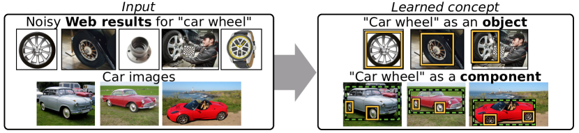
Figure 1: Our goal is to learn the semantic structure of objects automatically using Web supervision. For example, given noisy images obtained by querying an Internet search engine for “car wheel” and for “cars”, we aim at learning the “car wheel” concept, and its dual nature: as an object in its own right, and as a component of another object.

A byproduct of our method is a large collection of images annotated with objects, semantic parts, and their geometric relationships, that we refer to as a visual semantic atlas (section 4). This atlas allows to visually navigate images based on conceptual and geometric relations. It also emphasizes the dual nature of parts, as components of an object and as semantic categories, by naturally bridging images that zooms on a part or that contain the object as a whole.

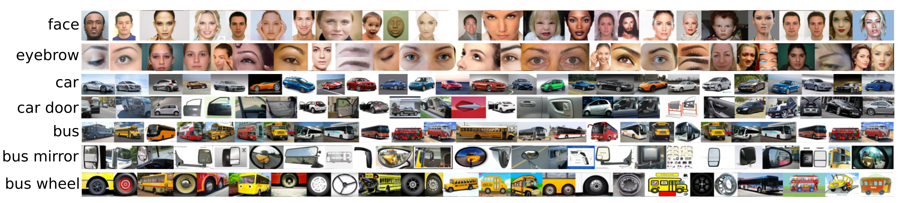
Figure 2: Top images retrieved from an Internet search engine for some example queries. Note that part results are more noisy than full object results (the remaining collected images get even noisier, not shown here).

1.1 Related work

Our work touches on several active research areas: localizing objects with weak supervision, learning with Web images, and discovering or learning mid-level features and object parts.

Localizing objects with weak supervision. When training models to localize objects or parts, it is impractical to expect large quantities of bounding box annotations. Recent works have tackled the localization problem with only image-level annotations. Among them, weakly supervised object localization methods [10, 11, 12, 13, 14, 15, 16] assume for each image a list of every object type it contains. In the co-detection [17, 18, 19, 20] and co-segmentation [21, 22, 23, 24] problems, the algorithm is given a set of images that all contain at least one instance of a particular object. They differ in their output: co-detection predicts bounding boxes, while segmentation predicts pixel-level masks. Yet, co-detection, co-segmentation and weakly-supervised object localization (WSOL) are different flavors of the localization problem with weak supervision. For co-detection and WSOL, the task is nearly always formulated as a multiple instance learning (MIL) problem [10, 11, 25, 19, 26]. The formulation in [14, 15] departs from MIL by leveraging the strong annotations for some categories to transfer knowledge to the remaining categories. A few approaches model images using topic models [13, 20]. Recently, CNN architectures were also proved to work well in weakly supervised scenarios [27]. We will compare with [27] in the experiments section. None of these works have considered semantic parts. Closer to our work, the method of [28] proposes unsupervised discovery of dominant objects using part-based region matching. Because of its unsupervised process, this method is not suited to name the discovered objects or matched regions, and hence lack semantics. Yet we also compare with this approach in our experiments.

Learning from Web supervision. Most previous works [29, 30, 31, 32] that learn from noisy Web images have focused on image classification. Usually, they adopt an iterative approach that jointly learns models and finds clean examples of a target concept. Only few works have looked at the problem of localization. Some approaches [33, 24] discover common segments within a large set of Web images, but they do not quantitatively evaluate localization. The recent method of [34] localizes objects with bounding boxes, and evaluate the learnt models, but as the previous two, it does not consider object parts. Closer to our work, [35] aims at discovering common sense knowledge relations between object categories from Web images, some of which correspond to the “part-of” relation. In the process of organizing the different appearance variations of Webly mined concepts, [36] uses a “vocabulary of variance” that may include part names, but those are not associated to any geometry.

Unsupervised parts, mid-level features, and semantic parts. Objects are modeled using the notion of parts since the early work on pictorial structure [37], in the constellation [38] and ISM [39] models, and more recently the DPM [9]. Parts are most commonly defined as localized components with consistent appearance and geometry in an object. All these works have in common to discover object parts without naming them. In practice, only some of these parts have an actual semantic interpretation. Mid-level features [40, 41, 42, 43, 44, 45] are discriminative [43, 46] or rare [40] blocks, which are leveraged for object recognition. Again, these parts lack semantic. The non-semantic anchors that we use share similarities with [47] and [44], that we discuss in section 2.2. Semantic parts have triggered recent interest [48, 49, 50]. These works require strong annotations in the form of bounding boxes [48] or segmentation masks [49, 50] at the part level. Here we depart from existing work and aim at mining semantic nameable parts with as little supervision as possible.

2 Method

This section introduces our method to learn semantic parts using weak supervision from Web sources. The key challenge is that search engines, when queried for object parts, return many outliers containing other parts as well, the whole object, or entirely unrelated things (fig. 2). In this setting, standard weakly-supervised detection approaches fail (section 3). Our solution is a novel, robust, and flexible representation of object parts (section 2.1) that uses the output of a simple but very effective non-semantic part discovery algorithm (section 2.2).

2.1 Learning semantic parts using non-semantic anchors

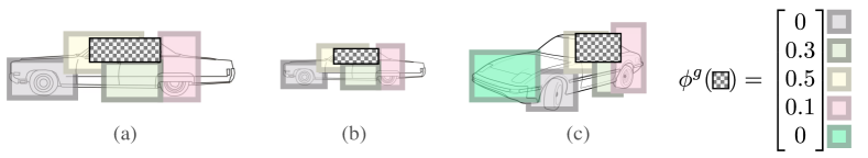
Figure 3: Anchor-induced geometry. (a) A set of anchors (light boxes) are obtained from a large number of unsupervised non-semantic part detectors. The geometry of a semantic part or object is then expressed as a vector $\phi^{g}$ of anchor overlaps. (b) The representation is scale and translation invariant. (c) The representation implicitly codes for multiple aspects.

In this section, we first flesh out our method for weakly-supervised part learning and then dive into the theoretical justification of our choices.

MIL: baseline, context, and geometry-aware. As standard in weakly-supervised object detection, our method starts from the Multiple Instance Learning (MIL) [51] algorithm. Let $\mathbf{x}_{i}$ be an image and let $\mathcal{R}(\mathbf{x}_{i})$ be a shortlist of image regions $R$ that are likely to contain objects or parts, obtained for instance using selective search [52]. Each image $\mathbf{x}_{i}$ can be either positive $y_{i}=+1$ if it is deemed to contain a certain part or negative $y_{i}=-1$ if not. MIL fits to this data a (linear) scoring function $\langle\phi(\mathbf{x}_{i}|R),\mathbf{w}\rangle$, where $\mathbf{w}$ is a vector of parameters and $\phi(\mathbf{x}_{i}|R)\in\mathbb{R}^{d}$ is a descriptor of the region $R$ of image $\mathbf{x}_{i}$, by minimizing:

$$\min_{\mathbf{w}\in\mathbb{R}^{d}}\frac{\lambda}{2}\|\mathbf{w}\|^{2}+\frac{1}{n}\sum_{i=1}^{n}\max\{0,1-y_{i}\max_{R\in\mathcal{R}(\mathbf{x}_{i})}\langle\phi(\mathbf{x}_{i}|R),\mathbf{w}\rangle\}$$ (1)

In practice, eq. 1 is optimized by alternatively selecting the maximum scoring region for each image (also known as “re-localization”) and optimizing $\mathbf{w}$ for a fixed selection of the regions. In this manner, MIL should automatically discover regions that are most predictive of a given label, and which therefore should correspond to the sought visual entity (object or semantic part). However, this process may fail if descriptors are not sufficiently strong.

For baseline MIL the descriptor $\phi(\mathbf{x}|R)=\phi^{a}(\mathbf{x}|R)\in\mathbb{R}^{d_{a}}$ captures the region’s appearance. A common improvement is to extend this descriptor with context information by appending a descriptor of a region $R^{\prime}=\mu(R)$ surrounding $R$, where $\mu(R)$ isotropically enlarges $R$; thus in context-aware MIL, $\phi(\mathbf{x}|R)=\operatorname{stack}(\phi^{a}(\mathbf{x}|R),\phi^{a}(\mathbf{x}|\mu(R)))$.

Neither baseline or context-aware MIL leverage the fact that objects have a well-defined geometric structure, which significantly constrains the search space for parts. DPM uses such constraints, but as a fixed set of geometric relationships between part pairs that are difficult to learn when examples are extremely noisy. Furthermore, DPM-like approaches learn the most visually-stable parts, which often are not the semantic ones.

We propose here an alternative method that captures geometry indirectly, on top of a rich set of unsupervised mid-level non-semantic parts $\{p_{1},...,p_{K}\}$, which we call anchors (fig. 3). Let us assume that, given an image $\mathbf{x}$, we can locate the (selective search) regions $R_{p_{k},\mathbf{x}}$ containing each anchor $p_{k}$. We define the following geometric embedding $\phi^{g}$ of a region $R$ with respect to the anchors:

$$\phi^{g}(\mathbf{x}|R)=\begin{bmatrix}\rho(R,R_{p_{1},\mathbf{x}})\\ \vdots\\ \rho(R,R_{p_{K},\mathbf{x}})\end{bmatrix}.$$ (2)

Here $\rho$ is a measure such as intersection-over-union (IoU) that tells whether two regions overlap. By choosing a function $\rho$ such as IoU which is invariant to scaling, rotation, and translation of the regions, so is the embedding $\phi^{g}$. Hence, as long as anchors stay attached to the object, $\phi^{g}(\mathbf{x}|R)$ encodes the location of $R$ relative to an object-centric frame. This representation is robust because, even if some anchors are missing or misplaced, the vector $\phi^{g}(\mathbf{x}|R)$ is not greatly affected. The geometric encoding $\phi^{g}(\mathbf{x}|R)$ is combined with the appearance descriptor $\phi^{a}(\mathbf{x}|R)$ in a joint appearance-geometric embedding

$$\phi^{ag}(\mathbf{x}|R)=\phi^{a}(\mathbf{x}|R)\otimes\phi^{g}(\mathbf{x}|R)$$ (3)

where $\otimes$ is the Kronecker product. After vectorization, this vector is used as a descriptor $\phi(\mathbf{x}|R)=\phi^{ag}(\mathbf{x}|R)$ of region $R$ in geometry-aware MIL. The next few paragraphs discuss its properties.

Modeling multiple parts. Plugging $\phi^{ag}$ of eq. (3) into eq. (1) of MIL results in the scoring function $\langle\mathbf{w},\phi^{ag}(\mathbf{x}|R)\rangle=\sum_{k=1}^{K}\langle\mathbf{w}_{k},\phi^{a}(\mathbf{x}|R)\rangle\rho(R,R_{p_{k},\mathbf{x}})$ which interpolates between $K$ appearance models based on how the region $R$ is geometrically related to the anchors $R_{p_{k},\mathbf{x}}$. In particular, by selecting different anchors this model may capture simultaneously the appearance of all parts of an object. In order to control the capacity of the model, the smoothness of the interpolator can be increased by replacing IoU with a softer version, which we do next.

Smoother overlap measure. The IoU measure is a special case of the following family of PD kernels (proof in the appendix):

Theorem 2.1

Let $R$ and $Q$ be vectors in a Hilbert $\mathcal{H}$ space such that $\langle R,R\rangle+\langle Q,Q\rangle-\langle R,Q\rangle>0$. Then the function $\rho(R,Q)=\frac{\langle R,Q\rangle}{\langle R,R\rangle+\langle Q,Q\rangle-\langle R,Q\rangle}$ is a positive definite kernel.

The IoU is obtained when $R$ and $Q$ are indicator functions of the respective regions (because $\langle R,Q\rangle=\int R(x,y)Q(x,y)\,dx\,dy=|R\cap Q|$). This suggests a simple modification to construct a Soft IoU (SIoU) version of the latter. For a region $R=[x_{1},x_{2}]\times[y_{1},y_{2}]$, the indicator can be written as $R(x,y)=H(x-x_{1})H(x_{2}-x)H(y-y_{1})H(y_{2}-y)$ where $H(z)=[z\geq 0]$ is the Heaviside step function. SIoU is obtained by replacing the indicator by the smoother function $H_{\alpha}(z)=\exp(\alpha z)/(1+\exp(\alpha z))$ instead. Note that SIoU is non-zero even when regions do not intersect.

Theorem 2.1 provides also an interpretation of the geometric embedding $\phi^{g}$ of eq. (2) as a vector of region coordinates relative to the anchors. In fact, its entries can be written as $\rho(R,R_{p_{k},\mathbf{x}})=\langle\psi_{\text{SIoU}}(R),\psi_{\text{SIoU}}(R_{p_{k},\mathbf{x}})\rangle$ where $\psi_{\text{SIoU}}(R)\in\mathcal{H}_{\text{SIoU}}$ is the linear embedding (feature map) induced by the kernel $\rho$.

Modeling multiple aspects. So far, we have assumed that all parts are always visible; however, anchors also provide a mechanism to deal with the multiple aspects of 3D objects. As depicted in fig. 3.c, as the object rotates out of plane, anchors naturally appear and disappear, therefore activating and de-activating aspect-specific components in the model. In turn, this allows to model viewpoint-specific parts or appearances. In practice, we extract the $L$ highest scoring detections $R_{l}$ of the same anchor $p_{k}$, and keep the one closest to $R$.

In order to allow anchors to turn off in the model, the geometric embedding is modified as follows. Let $s_{k}(R_{l}|\mathbf{x})$ be the detection score of anchor $k$ in correspondence of the region $R_{l}$; then

$$\rho(R,R_{p_{k},\mathbf{x}})=\max_{l\in\{1,\dots,L\}}\operatorname{SIoU}(R,R_{l})\times\max\{0,s_{k}(R_{l}|\mathbf{x})\}.$$ (4)

If the anchor is never detected ($s_{k}(R_{l}|\mathbf{x})\leq 0$ for all $R_{l}$) then $\rho(R,R_{p_{k},\mathbf{x}})=0$. Furthermore, this expression also disambiguates ambiguous anchor detections by picking the one closest to $R$. Note that in eq. (4) one can still interpret the factors $\operatorname{SIoU}(R,R_{l})$ as projections $\langle\psi_{\text{SIoU}}(R),\psi_{\text{SIoU}}(R_{l})\rangle$.

Relation to DPM. DPM is also a MIL method using a joint embedding $\phi^{\text{DPM}}(\mathbf{x}|R_{1},\dots,R_{K})$ that codes simultaneously for the appearance of $K$ parts and their pairwise geometric relationships. Our Webly-supervised learning problem requires a representation that can bridge object-focused images (where several parts are visible together as components) and part-focused images (where parts are regarded as objects in their own right). This is afforded by our embedding $\phi^{ag}(\mathbf{x}|R)$ but not by the DPM one. Besides bridging parts as components and parts as objects, our embedding is very robust (important in order to deal with very noisy training labels), automatically codes for multiple object aspects, and bridges unsupervised non-semantic parts (the anchors) with semantic ones.

2.2 Anchors: weakly-supervised non-semantic parts

The geometric embedding in the previous section leverages the power of an intermediate representation: a collection of anchors $\{p_{k}\}_{k=1}^{K}$, learned automatically using weak supervision. While there are many methods to discover discriminative non-semantic mid-level parts from image collections (section 1.1), here we propose a simple alternative that, empirically, works better in our context.

We learn the anchors using a formulation similar to the MIL objective (eq. (1)):

$$\min_{\boldsymbol{\omega}_{1},\dots,\boldsymbol{\omega}_{K}}\sum_{i=1}^{K}\left[\frac{\lambda}{2}\|\boldsymbol{\omega}_{k}\|^{2}-\frac{1}{n}\sum_{i=1}^{n}y_{i}\left[\max_{R\in\mathcal{R}(\mathbf{x}_{i})}\langle\phi^{a}(\mathbf{x}_{i}|R),\boldsymbol{\omega}_{k}\rangle\right]_{+}\right]+\gamma\sum_{k\not=q}\left\langle\frac{\boldsymbol{\omega}_{k}}{\|\boldsymbol{\omega}_{k}\|},\frac{\boldsymbol{\omega}_{q}}{\|\boldsymbol{\omega}_{q}\|}\right\rangle^{2},$$ (5)

where $[z]_{+}=\max\{0,z\}$. Intuitively, anchors are learnt as discriminative mid-level parts using weak supervision. Anchor scores $s_{k}(R|\mathbf{x})=\langle\phi^{a}(\mathbf{x}|R),\boldsymbol{\omega}_{k}\rangle$ are parametrized by vectors $\boldsymbol{\omega}_{1},\dots,\boldsymbol{\omega}_{K}$; the first term in eq. 5 is akin to the baseline MIL formulation of section 2.1 and encourages each anchor $p_{k}$ to score highly in images $\mathbf{x}_{i}$ that contain the object ($y_{i}=+1$) and to be inactive otherwise ($y_{i}=-1$). The last term is very important and encourages the learned models $\{\boldsymbol{\omega}_{k}\}_{k=1}^{K}$ to be mutually orthogonal, enforcing diversity. Note that anchors use the pure appearance-based region descriptor $\phi^{a}(\mathbf{x})$ since the geometric-aware descriptor $\phi^{ag}(\mathbf{x})$ can be computed only once anchors are available. Optimization uses stochastic gradient descent with momentum.

This formulation is similar to the MIL approach of [47] which, however, does not contain the orthogonality term. When this term is removed, we observed that the solution degenerates to detecting the most prominent object in an image. [41] uses instead a significantly more complex formulation inspired by mode seeking; in practice we opted for our approach due to its simplicity and effectiveness.

2.3 Incorporating strong annotations in MIL

While we are primarily interested in understanding whether semantic object parts can be learned from Web sources alone, in some cases the precise definition of the extent of a part is inherently ambiguous (e.g. what is the extent of a “human nose”?). Different benchmark datasets may use somewhat different definition of these concepts, making evaluation difficult. In order to remove or at least reduce this dataset-dependent ambiguity, we also explore the idea of using a single strongly annotated example to fix this degree of freedom.

Denote by $(\mathbf{x}_{a},R_{a})$ the single strongly-annotated example of the target part. This is incorporated in the MIL formulation, eq. (1), by augmenting the score with a factor that compares the appearance of a region to that of $R_{a}$:

$$\langle\phi(\mathbf{x}_{i}|R),\mathbf{w}\rangle\times\begin{cases}\frac{1}{C}\exp\beta\langle\phi^{a}(\mathbf{x}_{i}|R),\phi^{a}(\mathbf{x}_{a}|R_{a})\rangle,&y_{i}=+1,\\ 1,&y_{i}=-1.\end{cases}$$ (6)

where $C=\operatornamewithlimits{avg}_{i:y_{i}=+1}\exp\beta\langle\phi^{a}(\mathbf{x}_{i}|R),\phi^{a}(\mathbf{x}_{a}|R_{a})\rangle$ is a normalizing constant. In practice, this is used only during re-localization rounds of the training phase to guide spatial selection; at test time, bounding boxes are scored solely by the model of eq. (1) without the additional term. Other formulations, that may use a mixture of strongly and Webly supervised examples, are also possible. However, this is besides our focus, which is to see whether parts are learnable from the Web automatically, and the single supervision is only meant to reduce the ambiguity in the task for evaluation.

3 Experiments

This section thoroughly evaluates the proposed method. Our main evaluation is a comparison with existing state-of-the-art techniques on the task of Webly-supervised semantic part learning. In section 3.1 we show that our method is substantially more accurate than existing alternatives and, in some cases, close to fully-supervised part learning.

Having established that, we then evaluate the weakly-supervised mid-level part learning (section 2.2) that is an essential part of our approach. It compares favorably in terms of simplicity, scalability, and accuracy against existing alternatives for discriminability as well as spatial matching of object categories (table 4).

Datasets. The Labeled Face Parts in the Wild (LFPW) dataset [53] contains about 1200 face images annotated with outlines for landmarks. Outlines are converted into bounding box annotations and images with missing annotations are removed from the test set. These test images are used to locate the following entities: face, eye, eyebrow, nose, and mouth.

The PascalParts dataset [49] augments the PASCAL VOC 2010 dataset with segmentation masks for object parts. Segmentation masks are converted into bounding boxes for evaluation. Parts of the same type (e.g. left and right wheels) are merged in a single entity (wheel). Objects marked as truncated or difficult are not considered for evaluation. The evaluation focuses on the bus and car categories with 18 entity types overall: car, bus, and their door, front, headlight, mirror, rear, side, wheel, and window parts. This dataset is more challenging, as entities have large intra-class appearance and pose variations. The evaluation is performed on images from the validation set that contain at least one object instance. Furthermore, following [50], object occurrences are roughly localized before detecting the parts using their localization procedure. Finally, objects whose bounding box larger side is smaller than 80 pixels are removed as several parts are nearly invisible below that scale.

The training sets from both datasets are utilized solely for training the fully supervised baselines (section 3.1), and they are not used by MIL approaches.

Experimental details. Regions are extracted using selective search [52], and described using $\ell_{2}$-normalized Decaf [54] fc6 features to compute the appearance embedding $\phi^{a}(\mathbf{x}|R)$. The context descriptor $\mu(R)$ is extracted from a region double the size of $R$. The joint appearance-geometric embedding $\phi^{ag}(\mathbf{x}|R)$ is obtained by first extracting the top $L=5$ non-overlapping detections of each anchor and then applying eqs. 4 and 3.

A separate mid-level anchor dictionary $\{p_{1},...,p_{K}\}$ is learnt for each object class using the Web images for all the semantic parts for the target object (including images of the object as a whole) as positive images and the background clutter images of [55] as negative ones. Eq. (5) is optimized using stochastic gradient descend (SGD) with momentum for 40k iterations, alternating between positive and negative images. We train 150 anchor detectors per object class.

MIL semantic part detectors are trained solely on the Web images and the background class of [55] is used as negative bag for all the objects. The first five relocalization rounds are performed using the appearance only and the following five use the joint appearance-geometry descriptor (the joint embedding performs better with these two distinct steps). The MIL $\lambda$ hyperparameter is set by performing leave-one-category-out cross-validation.

Web images for parts are acquired by querying the BING image search engine. For car and bus parts, the query concatenates the object and the part names (e.g. ”car door”). For face parts, we do not use the object name. We retrieve 500 images of the class corresponding to the object itself and 100 images of all other semantic part classes.

3.1 Webly supervised localization of objects and semantic parts

This section evaluates the detection performance of our approach. We gradually incorporate the proposed improvements, i.e. the context descriptor (C) and the geometrical embedding (G) to the basic MIL baseline (B) as defined in section 2.1 and monitor their impact.

We compare our method to the state-of-the-art co-localization algorithm of Cho et al. [28] and the state-of-the-art weakly supervised detection method from Bilen and Vedaldi [27]. To detect a given part with [28], we run their code on all images that contain that part (e.g. for co-localizing eyes we consider face and eye images). As reference, we also report a fully supervised detector, trained using bounding-boxes from the training set, for all objects and parts (F). For this, we use the R-CNN method of [2] on top of the same features used in MIL.

We mainly report the Average Precision (AP) per part/object class and its average (mAP) over all parts in each class. We also report the CorLoc (for correct localization) measure, as it is often used in the co-localization literature [56, 17]. As most parts in both datasets are relatively small, following [49], the $\operatorname{IoU}$ threshold for correct detection is set to 0.4.

measure	mAP			averageCorLoc
Parent class	{face}	{car}	{bus}	{face}	{car}	{bus}
Cho et al. [28]	16.6	16.9	12.4	31.4	29.9	15.5
Bilen & Vedaldi [27]	2.7	12.0	4.7	7.2	15.3	6.7
B	20.6	29.1	22.7	22.0	38.1	29.4
B+C	22.4	27.3	21.4	29.1	37.6	28.4
B+G	29.0	34.1	23.3	33.1	45.5	31.5
B+C+G	44.9	34.4	23.0	52.5	47.8	29.6
F	53.7	51.2	48.2	60.5	62.9	63.8
F+C+G	61.4	60.3	54.1	67.8	71.8	66.0

Table 1: Part detection results averaged for the face, car, and bus parent classes. mAP and average CorLoc for the MIL baseline (B), our improved versions that use context (C), geometrical embedding (G) compared to the fully supervised R-CNN (F).

Class		door	rear	wheel	wind.	side	car	front	headl.	mirror	mean{car}
Web	B	0.4	10.8	34.9	3.6	63.1	92.6	55.2	0.7	0.3	29.1
	B+C	0.8	11.4	31.3	4.9	58.8	83.0	54.0	1.0	0.2	27.3
	B+G	0.7	11.8	47.9	22.7	71.3	97.8	54.5	0.2	0.2	34.1
	B+C+G	5.1	14.7	43.6	22.6	72.3	95.7	54.7	0.3	0.2	34.4
Full	F	17.0	39.0	66.3	53.3	83.2	95.1	75.9	25.3	5.5	51.2
	F+C+G	31.1	30.7	72.3	67.3	90.1	98.7	82.9	48.1	21.3	60.3

Table 2: Individual part detection results for car: APs for the MIL baseline (B), our improved versions that use context (C), geometrical embedding (G) and the different flavors of the fully supervised R-CNN (F).

Results. Table 1 reports the average AP and CorLoc over all parts of a given object class for all these methods. First, we observe that even the MIL baseline (B) outperforms off-the-shelf methods such as [28] and [27]. For [27], we have observed that the part detectors degrade to detecting subparts of semantic parts, suggesting that [27] lacks robustness to drastic scale variations and to the large amount of noise present in our dataset. Second, we see that using the geometric embedding (+G) always improves the baseline results by $1-10$ mAP points. On top of geometry, using context (+C) helps for face and car parts, but not for buses. Overall the unified embedding brings a large improvement for faces (+24.3 mAP) and for cars (+5.3 mAP) and more contained for buses (+0.6 mAP). Importantly, these improvements significantly reduce the gap between using noisy Web supervision and the fully supervised R-CNN (F); overall, Webly supervision achieves respectively 84%, 67%, and 48% of the performance of (F).

Last but not least, we extended the fully supervised R-CNN method with the joint appearance-geometry embedding and the context descriptor (F+C+G), which improves part detections by +7.7, +9.1, +5.9 mAP points respectively. This suggests that our representation may be applicable well beyond weakly supervised learning.

Table 2 shows per-part detection results for the car parts. We see that geometry helps for 6 parts out of 9. Out of the three remaining parts, two are cases for which the MIL baseline failed completely. In the less ambiguous fully-supervised scenario, the geometric embedding improves the performance in 8 out of 9 cases.

measure	mAP			averageCorLoc
Parent class	{face}	{car}	{bus}	{face}	{car}	{bus}
A	29.4 $\pm$ 2.6	25.1 $\pm$ 2.7	24.5 $\pm$ 2.7	38.2 $\pm$ 2.5	39.8 $\pm$ 3.2	39.6 $\pm$ 3.2
A+B	27.3 $\pm$ 3.1	33.3 $\pm$ 1.1	26.9 $\pm$ 1.3	34.6 $\pm$ 3.7	46.6 $\pm$ 1.5	40.0 $\pm$ 2.3
A+B+C	38.2 $\pm$ 3.1	32.4 $\pm$ 1.2	26.6 $\pm$ 1.6	51.7 $\pm$ 3.2	49.4 $\pm$ 1.5	43.9 $\pm$ 3.0
A+B+G	34.5 $\pm$ 4.3	35.7 $\pm$ 1.1	28.1 $\pm$ 1.2	43.5 $\pm$ 4.8	48.8 $\pm$ 1.6	42.2 $\pm$ 2.2
A+B+C+G	43.0 $\pm$ 3.6	36.4 $\pm$ 1.0	30.1 $\pm$ 1.8	54.7 $\pm$ 3.2	51.6 $\pm$ 1.6	45.9 $\pm$ 2.8

Table 3: Part detection results using a single strong annotation (A): mAP and average CorLoc for the MIL baseline (B), our improved versions that use context (C), geometrical embedding (G). Mean and standard deviation over 25 random annotations.

Leveraging a single annotation. As noted in section 2.3, one issue with weakly supervised part learning is the inherent ambiguity in the part extent, that may differ from dataset to dataset. Here we address the ambiguity by adding a single strong annotation to the mix using the method described in section 2.3. We asked an annotator to select 25 representative part annotations per part class from the training sets of each dataset. We retrain every part detector for each of the annotations and report mean and standard deviation of mAP. As a baseline, we also consider an exemplar detector trained using the single annotated example (A).

Results are reported in table 3. Compared to pure Web supervision (B+C+G) in table 1, the single annotation (A+B+C+G) does not help for faces, for which the proposed method was already working very well, but there is a +2 mAP point improvement for cars and +6.8 mAP for buses, which are more challenging. We also note that the complete method (A+B+C+G) is substantially superior to the exemplar detector (A).

3.2 Validation of weakly-supervised mid-level anchors

This section validates the mid-level anchors (section 2.2) against alternatives in terms of discriminative information content and its ability of establishing meaningful matches between images, which is a key requirement in our application.

Discriminative power of anchors. Since most of the existing methods for learning mid-level patches are evaluated in terms of discriminative content in a classification setting, we adopt the same protocol here. In particular, we evaluate the anchors as mid-level patches on the MIT Scene 67 indoor scene classification task [57]. The pipeline first learns 50 mid-level anchors for each of the 67 scene classes. Then, similar to [45], images are split into spatial grids (2x2 and 1x1) and described by concatenating the maximum scores attained by each anchor detector inside each bin of the grid. All the grid descriptors are then concatenated to form a global image descriptor which is $\ell_{2}$ normalized. 67 one-vs-rest SVM classifiers are trained on top of these descriptors. To be comparable with other methods, we consider both Decaf fc6 and VGG-VD fc7 [58] descriptors.

Table 4 contains the results of the classification experiment. Our weakly-supervised anchors clearly outperform other mid-level element approaches that are not based on CNN features [42, 41, 47, 46]. Among CNN based approaches, our method outperforms the state-of-the-art mid-level feature based method from [45] on both VGG-VD and Decaf features. Remarkably, using our part detectors improves over the baseline which uses the global image CNN descriptor (FC) by 13.8 and 8.7 average accuracy points for Decaf and VGG-VD features respectively. Compared to other methods which are not based on detecting mid-level elements, our pipeline outperforms state-of-the-art FV-CNN for Decaf features and is inferior for VGG-VD.

method	BoP† [42]	DMS† [41]	Jian et al.† [47]	RFDC† [46]	FC Decaf [54]	FC VGG-VD [58]
accuracy (%)	46.1	64.0	58.1	54.4	57.7	68.9
method	BoE† Decaf [45]	ours† Decaf	FV-CNN Decaf [59]	BoE† VGG-VD [45]	ours† VGG-VD	FV-CNN VGG-VD [59]
accuracy (%)	69.7	71.5	69.7	77.6	77.8	81.6

Table 4: Classification results on MIT Scenes [57]. Methods using mid-level elements are marked with ^†. For CNN-based approaches, features rely on Decaf or VGG-VD.

Ability of anchors to establish semantic matches. The previous experiment assessed favorably the mid-level parts in terms of discriminative content; however, in the embedding $\phi^{g}$, these are used as geometric anchors. Hence, here we validate the ability of the mid-level anchors to induce good semantic matches between pairs of images (before learning the semantic part models).

To perform semantic matching between a source image $x_{S}$ and a target image $x_{T}$, we consider each part annotation $R_{S}$ in the source and predict its best match $\hat{R}_{T}$ in the target. The quality of the match is evaluated by measuring the IoU between the predicted $\hat{R}_{T}$ and ground-truth $R_{T}$ part. When a part appears more than once (e.g. eyes often appear twice), we choose the most overlaping pair. Performance is reported by averaging the match IoU for all part occurrences and pairs of images in the test set, reporting the results for each object category.

Given a source part $R_{S}$, the joint appearance-geometry embedding (anchor-ag) is extracted for the source part $\phi^{ag}(\mathbf{x}_{S}|R_{S})$ and the target region $\hat{R}_{T}$ that maximizes the inner product $\langle\phi^{ag}(\mathbf{x}_{S}|R_{S}),\phi^{ag}(\mathbf{x}_{T}|\hat{R}_{T})\rangle$ is returned as the predicted match. We also compare anchor-g that uses only the geometric embedding $\phi^{g}(\mathbf{x}|R)$ and the baseline a that uses only the appearance embedding $\phi^{a}(\mathbf{x}|R)$.

We also compare two strong off-the-shelf baselines: DSP [60], state-of-the-art pairwise semantic matching method, and the method of [61], state-of-the-art for joint alignment. To perform box matching with [60] and [61] we fit an affine transformation to the disparity map contained inside a given source bounding box and apply this transform to move this box to the target image. Due to scalability issues, we were unable to apply [61] to the full dataset, so we perform this comparison on a random subset of 50 images.

Table 5 presents the results of our benchmark. On the small subset of 50 images the costly approach of [61] performs better than our embedding only on the LFPW faces, where the viewpoint variation is limited. On the car and bus categories our method outperforms [61] by 10% and 16% average IoU respectively. Our method is also consistently better than DSP [60] on both the small and full test set. We also note that the matching using geometric embeddings alone (anchor-g) achieves similar performance than the appearance-geometry matching (anchor-ag) which validates our intuition that the local geometry of an object is well-captured by the anchors.

		Matching method
Set	Parent class	anchor-ag	anchor-g	a	Flowweb [61]	DSP [60]
50 images	{car}	0.36	0.36	0.31	0.34	0.23
	{bus}	0.37	0.36	0.31	0.31	0.22
	{face}	0.41	0.39	0.33	0.43	0.19
Full	{car}	0.36	0.36	0.30	-	0.22
	{bus}	0.35	0.35	0.29	-	0.21
	{face}	0.41	0.39	0.34	-	0.21

Table 5: Semantic matching. For every parent class, we report average overlap (IoU) over all semantic parts. The face class results are obtained on the LFPW dataset while bus and car results come from the PascalParts dataset.

4 An atlas for visual semantic

As a byproduct of Webly-supervised learning, our method annotates the Web images with semantic parts. By endowing an image dataset with such concepts, we show here that it is possible to browse these annotated images. All of this composes our visual semantic atlas (see a subset of the atlas in Figure 4) that allows to navigate from one image to another, even between an image of a full object and a zoomed-in image of one of its parts.

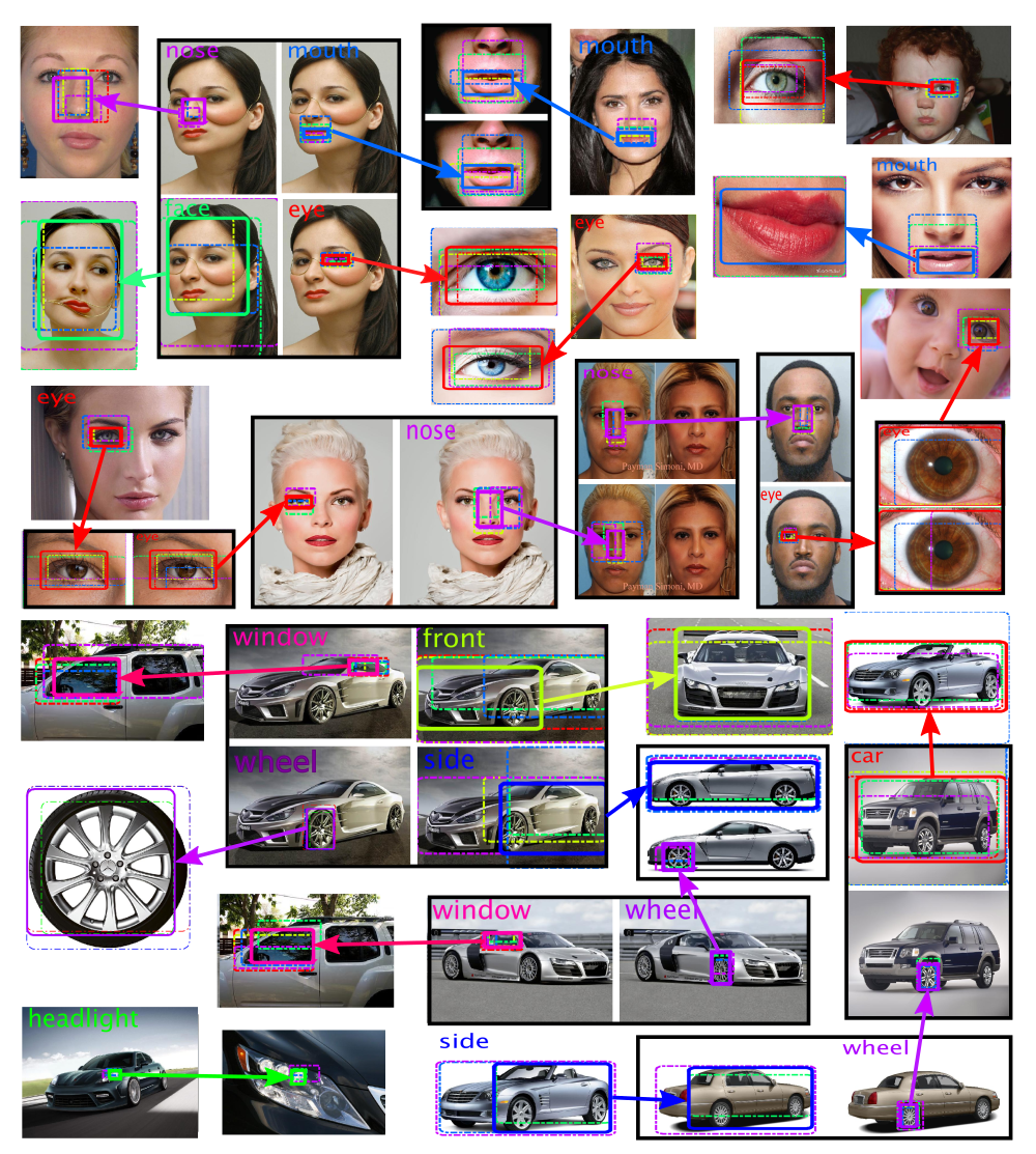
Figure 4: Navigating the visual semantic atlas. Each pair of solid bounding boxes connected by an arrow denotes a preselected part bounding box (near the starting point of an arrow) as detected by our algorithm and the most similar semantic match (the endpoint of the arrow). The best matching bounding box is the detection with highest appearance-geometry descriptor similarity among all the detections in our database of web images. The dashed boxes denote anchors that contributed the most to the similarity. Please note that the matching gracefully occurs across scales.

5 Conclusions

We have proposed a novel method for learning about objects, their semantic parts, and their geometric relationships, from noisy Web supervision. This is achieved by first learning a weakly supervised dictionary of mid-level visual elements which define a robust object-centric coordinate frame. Such property theoretically motivates our approach. The geometric projections are then used in a novel appearance-geometry embedding that improves learning of semantic object parts from noisy Web data. We showed improved performance over co-localization [28], deep weakly supervised approach [27] and a MIL baseline on all benchmarked datasets. Extensive evaluation of our proposed mid-level elements shows comparable results to state-of-the-art in terms of their discriminative power and superior results in terms of the ability to establish semantic matches between images. Finally, our method also provides a visually intuitive way to navigate Web images and predicted annotations.

Acknowledgments.

We are grateful for support by XRCE and ERC StG 638009-IDIU.

Appendix 0.A Appendix

Proof (Proof of Theorem 1)

The function $\langle R,Q\rangle$ is the linear kernel, which is PD. This kernel is multiplied by the factor $-1/\bar{k}$ where $\bar{k}(R,Q)=\langle R,Q\rangle-\langle R,R\rangle-\langle Q,Q\rangle$; if this factor is also a PD kernel, then the result holds as the product of PD kernels is PD. According to Lemma 3.2 of [62], $-1/\bar{k}$ is PD if, and only if, $\bar{k}$ is strictly negative (point-wise) and conditionally definite positive (CDP). The first condition is part of the assumptions. To show the second condition that $\bar{k}$ is CDP pick $n$ vectors $R_{1},\dots,R_{n}$ and real numbers $c_{1},\dots,c_{n}$ summing to zero $c_{1}+\dots+c_{n}=0$; then

$$\sum_{ij}c_{i}\bar{k}(R_{i},Q_{i})c_{j}=\sum_{ij}c_{i}\langle R_{i},Q_{j}\rangle c_{j}\geq 0$$

where we used the fact that the terms $\langle R_{i},R_{i}\rangle$ cancel out and the fact that $\langle R_{i},Q_{j}\rangle$ is PD.

References

- [1] Krizhevsky, A., Sutskever, I., Hinton, G.E.: Imagenet classification with deep convolutional neural networks. In: Proc. NIPS. (2012)
- [2] Girshick, R., Donahue, J., Darrell, T., Malik, J.: Rich feature hierarchies for accurate object detection and semantic segmentation. In: Proc. CVPR. (2014)
- [3] Frome, A., Corrado, G.S., Shlens, J., Bengio, S., Dean, J., Ranzato, M.A., Mikolov, T.: Devise: A deep visual-semantic embedding model. In: Proc. NIPS. (2013)
- [4] Karpathy, A., Joulin, A., Fei-Fei, L.: Deep fragment embeddings for bidirectional image-sentence mapping. In: Proc. NIPS. (2014)
- [5] Simonyan, K., Zisserman, A.: Two-stream convolutional networks for action recognition in videos. In: Proc. NIPS. (2014)
- [6] Russakovsky, O., Deng, J., Su, H., Krause, J., Satheesh, S., Ma, S., Huang, Z., Karpathy, A., Khosla, A., Bernstein, M., Berg, A.C., Fei-Fei, L.: ImageNet Large Scale Visual Recognition Challenge. IJCV (2015) 1–42
- [7] Deng, J., Dong, W., Socher, R., Li, L.J., Li, K., Fei-Fei, L.: ImageNet: A Large-Scale Hierarchical Image Database. In: Proc. CVPR. (2009)
- [8] Fischler, M.A., Elschlager, R.A.: The representation and matching of pictorial structures. IEEE Trans. Comput. 22(1) (January 1973) 67–92
- [9] Felzenszwalb, P.F., Girshick, R.B., McAllester, D., Ramanan, D.: Object detection with discriminatively trained part based models. PAMI 32(9) (2010) 1627–1645
- [10] Nguyen, M.H., Torresani, L., de la Torre, F., Rother, C.: Weakly supervised discriminative localization and classification: a joint learning process. In: Proc. ICCV. (2009)
- [11] Pandey, M., Lazebnik, S.: Scene recognition and weakly supervised object localization with deformable part-based models. In: Proc. ICCV. (2011)
- [12] Deselaers, T., Alexe, B., Ferrari, V.: Weakly supervised localization and learning with generic knowledge. Proc. ICCV (2012)
- [13] Wang, C., Ren, W., Huang, K., Tan, T.: Weakly supervised object localization with latent category learning. In: Proc. ECCV. (2014)
- [14] Hoffman, J., Guadarrama, S., Tzeng, E.S., Hu, R., Donahue, J., Girshick, R., Darrell, T., Saenko, K.: Lsda: Large scale detection through adaptation. In Ghahramani, Z., Welling, M., Cortes, C., Lawrence, N., Weinberger, K., eds.: Proc. NIPS. (2014)
- [15] Hoffman, J., Pathak, D., Darrell, T., Saenko, K.: Detector discovery in the wild: Joint multiple instance and representation learning. In: Proc. CVPR. (2015)
- [16] Cinbis, R.G., Verbeek, J., Schmid, C.: Weakly Supervised Object Localization with Multi-fold Multiple Instance Learning. PAMI (September 2015)
- [17] Joulin, A., Tang, K., Fei-Fei, L.: Efficient image and video co-localization with frank-wolfe algorithm. In: Proc. ECCV. (2014)
- [18] Tang, K., Joulin, A., Li, L.J., Fei-Fei, L.: Co-localization in real-world images. In: Proc. CVPR. (2014)
- [19] Ali, K., Saenko, K.: Confidence-rated multiple instance boosting for object detection. In: Proc. CVPR. (2014)
- [20] Shi, Z., Hospedales, T., Xiang, T.: Bayesian joint modelling for object localisation in weakly labelled images. PAMI 37(10) (Oct 2015) 1959–1972
- [21] Joulin, A., Bach, F., Ponce, J.: Efficient optimization for discriminative latent class models. In: Proc. NIPS. (2010)
- [22] Vicente, S., Rother, C., Kolmogorov, V.: Object cosegmentation. In: Proc. CVPR. (2011)
- [23] Joulin, A., Bach, F., Ponce, J.: Multi-class cosegmentation. In: Proc. CVPR. (2012)
- [24] Rubinstein, M., Joulin, A., Kopf, J., Liu, C.: Unsupervised joint object discovery and segmentation in internet images. Proc. CVPR (2013)
- [25] Song, H.O., Girshick, R., Jegelka, S., Mairal, J., Harchaoui, Z., Darrell, T.: On learning to localize objects with minimal supervision. In: Proc. ICML. (2014)
- [26] Li, Q., Wu, J., Tu, Z.: Harvesting mid-level visual concepts from large-scale internet images. In: Proc. CVPR. (2013)
- [27] Bilen, H., Vedaldi, A.: Weakly supervised deep detection networks. arXiv preprint arXiv:1511.02853 (2015)
- [28] Cho, M., Kwak, S., Schmid, C., Ponce, J.: Unsupervised Object Discovery and Localization in the Wild: Part-based Matching with Bottom-up Region Proposals. In: Proc. CVPR. (2015)
- [29] Fergus, R., Fei-Fei, L., Perona, P., Zisserman, A.: Learning object categories from google”s image search. In: Proc. ICCV. (2005) 1816–1823
- [30] Parkhi, O.M., Vedaldi, A., Zisserman, A.: On-the-fly specific person retrieval. In: International Workshop on Image Analysis for Multimedia Interactive Services, IEEE (2012)
- [31] Schroff, F., Criminisi, A., Zisserman, A.: Harvesting image databases from the web. In: Proc. ICCV. (2007)
- [32] Tsai, D., Jing, Y., Liu, Y., Rowley, H., Ioffe, S., Rehg, J.: Large-scale image annotation using visual synset. In: Proc. ICCV. (2011) 611–618
- [33] Kim, G., Xing, E.P.: On Multiple Foreground Cosegmentation. In: Proc. CVPR. (2012)
- [34] Chen, X., Gupta, A.: Webly supervised learning of convolutional networks. In: Proc. ICCV. (2015)
- [35] Chen, X., Shrivastava, A., Gupta, A.: Neil: Extracting visual knowledge from web data. In: Proc. ICCV. (2013)
- [36] Divvala, S.K., Farhadi, A., Guestrin, C.: Learning everything about anything: Webly-supervised visual concept learning. In: Proc. CVPR. (2014)
- [37] Felzenszwalb, P.F., Huttenlocher, D.P.: Pictorial structures for object recognition. IJCV 61 (2003) 2005
- [38] Fergus, R., Perona, P., Zisserman, A.: Object class recognition by unsupervised scale-invariant learning. In: Proc. CVPR. Volume 2. (June 2003) 264–271
- [39] Leibe, B., Leonardis, A., Schiele, B.: Robust object detection with interleaved categorization and segmentation. IJCV 77(1-3) (2008) 259–289
- [40] Singh, S., Gupta, A., Efros, A.A.: Unsupervised discovery of mid-level discriminative patches. In: Proc. ECCV. (2012)
- [41] Doersch, C., Gupta, A., Efros, A.A.: Mid-level visual element discovery as discriminative mode seeking. In: Proc. NIPS. (2013)
- [42] Juneja, M., Vedaldi, A., Jawahar, C.V., Zisserman, A.: Blocks that shout: Distinctive parts for scene classification. In: Proc. CVPR. (2013)
- [43] Endres, I., Shih, K.J., Jiaa, J., Hoiem, D.: Learning collections of part models for object recognition. In: Proc. CVPR. (2013)
- [44] Doersch, C., Gupta, A., Efros, A.A.: Unsupervised visual representation learning by context prediction. In: Proc. ICCV. (2015)
- [45] Li, Y., Liu, L., Shen, C., van den Hengel, A.: Mid-level deep pattern mining. In: Computer Vision and Pattern Recognition (CVPR), 2015 IEEE Conference on, IEEE (2015) 971–980
- [46] Bossard, L., Guillaumin, M., Van Gool, L.: Food-101–mining discriminative components with random forests. In: Proc. ECCV. (2014)
- [47] Sun, J., Ponce, J.: Learning dictionary of discriminative part detectors for image categorization and cosegmentation. Submitted to International Journal of Computer Vision, under minor revision (2015)
- [48] Zhang, N., Donahue, J., Girshick, R., Darrell, T.: Part-based R-CNNs for fine-grained category detection. In: Proc. ECCV. (2014)
- [49] Chen, X., Mottaghi, R., Liu, X., Fidler, S., Urtasun, R., Yuille, A.: Detect what you can: Detecting and representing objects using holistic models and body parts. In: Proc. CVPR. (2014)
- [50] Wang, P., Shen, X., Lin, Z.L., Cohen, S., Price, B.L., Yuille, A.L.: Joint object and part segmentation using deep learned potentials. In: Proc. ICCV. (2015)
- [51] Dietterich, T.G., Lathrop, R.H., Lozano-Pérez, T.: Solving the multiple instance problem with axis-parallel rectangles. Artificial Intelligence 89(1-2) (1997) 31 – 71
- [52] Uijlings, J., van de Sande, K., Gevers, T., Smeulders, A.: Selective search for object recognition. IJCV (2013)
- [53] Belhumeur, P.N., Jacobs, D.W., Kriegman, D.J., Kumar, N.: Localizing parts of faces using a consensus of exemplars. PAMI (2013)
- [54] Jia, Y., Shelhamer, E., Donahue, J., Karayev, S., Long, J., Girshick, R., Guadarrama, S., Darrell, T.: Caffe: Convolutional architecture for fast feature embedding. arXiv preprint arXiv:1408.5093 (2014)
- [55] Fei-Fei, L., Fergus, R., Perona, P.: Learning generative visual models from few training examples: An incremental bayesian approach tested on 101 object categories. CVIU (2007)
- [56] Deselaers, T., Alexe, B., Ferrari, V.: Localizing objects while learning their appearance. In: Proc. ECCV. (2010)
- [57] Quattoni, A., Torralba, A.: Recognizing indoor scenes. In: Proc. CVPR. (2009)
- [58] Simonyan, K., Zisserman, A.: Very deep convolutional networks for large-scale image recognition. arXiv:1409.1556 (2014)
- [59] Cimpoi, M., Maji, S., Vedaldi, A.: Deep filter banks for texture recognition and segmentation. In: Proc. CVPR. (2015)
- [60] Kim, J., Liu, C., Sha, F., Grauman, K.: Deformable spatial pyramid matching for fast dense correspondences. In: Proc. CVPR. (2013)
- [61] Zhou, T., Jae Lee, Y., Yu, S.X., Efros, A.A.: Flowweb: Joint image set alignment by weaving consistent, pixel-wise correspondences. In: Proc. CVPR. (2015)
- [62] Hein, M., Bousquet, O.: Hilbertian metrics and positive definite kernels on probability measures. In: Proc. AISTATS. (2005) 136–143