Robust clustering tools based on optimal transportation.

Abstract

A robust clustering method for probabilities in Wasserstein space is introduced. This new ‘trimmed $k$-barycenters’ approach relies on recent results on barycenters in Wasserstein space that allow intensive computation, as required by clustering algorithms. The possibility of trimming the most discrepant distributions results in a gain in stability and robustness, highly convenient in this setting. As a remarkable application we consider a parallelized estimation setup in which each of $m$ units processes a portion of the data, producing an estimate of $k$-features, encoded as $k$ probabilities. We prove that the trimmed $k$-barycenter of the $m\times k$ estimates produces a consistent aggregation. We illustrate the methodology with simulated and real data examples. These include clustering populations by age distributions and analysis of cytometric data.

AMS Subject Classification: Primary: 62H30, 62G35. Secondary: 62G20, 62P99.

Keywords: Cluster prototypes, $k$-barycenter, trimmed barycenter, robust aggregation, Wasserstein distance, Monge-Kantorovich problem, transport maps, trimmed distributions, parallelized inference, bragging, subragging, trimmed $k$-means algorithm.

1 Introduction.

Cluster Analysis belongs to the class of statistical procedures which are most required by practitioners. Even being simple to describe its scope, the fine details involved in the admissible shapes for clusters, the determination of the number of clusters and the habitual unexistence of exact algorithms to get the solution to relatively basic problems are difficulties intrinsic to the theory. But today, the enormous sizes of data sets and the increasing interest in structured complex data have also increased the interest and the inherent difficulties of the theory. On the whole, these facts make cluster analysis a challenging theory demanding new tools for the statistical analysis (see e.g. Hennig et al. [33] for the current state of the art and a panoramic view of the theory). In particular, data available as probability distributions are the focus of several disciplines such as demography or weather forecasting. In such cases, the natural space to describe or analyze the data must preserve their intrinsic structure, leading to consider abstract spaces where the elements are probability distributions. Although this would suffice to justify developing cluster analysis on these spaces, meta-analysis or aggregation of cluster analyses as well as parallelization of some cluster procedures can be also addressed from such a perspective, giving an unexplored added value to the theory. In fact, a main goal of this paper is to provide some tools for clustering in Euclidean spaces that arise by resorting to clustering in suitable metric spaces constituted by probability distributions.

By the way, $k$-means is an unquestionable reference in the clustering framework (see e.g. [33] to get a general perspective, in particular chapter 3 by B. Mirkin and chapter 5 by P. Awasthi and M.F. Balcan), being the simplest partitional clustering procedure generalizable to metric spaces. $k$-means in abstract spaces have been considered in Sverdrup-Thygeson [43], Cuesta-Albertos and Matrán [18], Pärna [39] and [40], Luschgy and Pagès [38] or Lember [36], although their settings do not properly cover the current objective. For a general metric space $(E,d)$, a $k$-mean or $k$-barycenter of the points $e_{1},\dots,e_{n}$ in $E,$ would be any set $\{\bar{m}_{1},\dots,\bar{m}_{k}\}\subset E$ verifying

$$\frac{1}{n}\sum_{i=1}^{n}\min_{j\in\{1,\dots,k\}}d^{2}(e_{i},\bar{m}_{j})\leq\frac{1}{n}\sum_{i=1}^{n}\min_{j\in\{1,\dots,k\}}d^{2}(e_{i},m_{j})\mbox{ for every set }\{m_{1},\dots,m_{k}\}\subset E.$$ (1)

The $k$-means procedure shares many of the merits of the mean, as well as its drawbacks, showing a very bad behaviour in presence of outliers or even bridge-points between clusters (see Cuesta-Albertos et al. [16]). Trimmed $k$-means were introduced in [16] in Euclidean spaces as a way of robustifying $k$-means. Given a trimming level $\alpha\in(0,1)$ and the set of $n$ points $e_{1},\dots,e_{n}$ in $E$, trimmed $k$-means (see Definition 2.1) look for a set $\{\bar{m}_{1},\dots,\bar{m}_{k}\}\subset E$ and a partition, $\mathcal{C}_{0},\mathcal{C}_{1},\dots,\mathcal{C}_{k}$, of $E$ that mimimize the trimmed dispersion, namely,

$$\frac{1}{n-[n\alpha]}\sum_{j=1}^{k}\sum_{e_{i}\in\mathcal{C}_{j}}d^{2}(e_{i},\bar{m}_{j}),$$ (2)

where $\mathcal{C}_{0}$, the set of trimmed elements, has $[n\alpha]$ elements. A minimizing set $\{\bar{m}_{1},\dots,\bar{m}_{k}\}$ will be called a trimmed $k$-barycenter of $e_{1},\dots,e_{n}$. We note that trimmed $k$-means in linear functional spaces have been considered in Cuesta-Albertos and Fraiman [17] and in García-Escudero and Gordaliza [27]. Our framework, in contrast, focuses on the case where each of $m$ units, possibly after some preprocessing, gives an estimated distribution, resulting in a meta-sample $\hat{P}_{1},\dots,\hat{P}_{m}$ of distributions or sets of distributions. These objects naturally live in $\mathcal{P}_{2}(\mathbb{R}^{d})$, the set of probabilities on $\mathbb{R}^{d}$ with finite second moment, which we endow with the $L_{2}$-Wasserstein distance, defined by

$$\mbox{$\mathcal{W}_{2}$}(P,Q):=\inf\left\{\left(\mbox{$\mathbf{E}$}\|U-V\|^{2}\right)^{1/2}:\ \mathcal{L}(U)=P,\ \mathcal{L}(V)=Q\right\},$$ (3)

where we use $\mathcal{L}(X)$ to denote the distribution law of a r.v. $X$ and $\mbox{$\mathbf{E}$}(X)$ for its mean.

In this work we consider $k$-barycenters and trimmed $k$-barycenters in this metric space, the $L_{2}-$Wasserstein space. This space has deserved notable interest by its connection with the celebrated Monge-Kantorovich transport problem, and provides a suitable setting for statistical analyses of structured data such as histograms, density functions or probabilities. For $k=1$, existence, uniqueness and characterizations of (1-)barycenters (or Fréchet means) in this space have been considered in Agueh and Carlier [1], while consistency results can be found in Le Gouic and Loubes [34] or Bigot and Klein [8] and trimmed barycenters have been introduced in Álvarez-Esteban et al [4]. Some recent additional references that resort to Wasserstein spaces with an statistical motivation are [5], [14], [15]. Being of indubitable mathematical interest, this approach could be considered just as the introduction of an additional abstract space where clustering of probabilities could be carried with more or less success. However, as already announced, through the paper we will stress mainly on other applications of the theory: We will address the consensus or aggregation of model-based cluster analyses through a kind of cluster prototypes, where the prototypes are probability distributions.

Focusing on the aggregation of structured data, there can hardly be any doubt (beyond its lack of robustness) about the good properties of the mean as a summary of a set of elements in a linear space. However, when we move to a shaped space the use of the mean can be unfeasible or produce undesirable effects (for example, the point-wise mean of several normal densities is no longer a normal density and the normal shape could be largely distorted). This kind of problem has been already pointed out in the statistical setting by several authors, notably by Kneip and Gasser [32], and more recently, proposing solutions based on Wasserstein spaces by Boissard et al. [10].

Consensus procedures in Cluster Analysis have a long story, but generally suffer from the lack of feasible ways to measure the similarity between several clustering proposals (see e.g. “A survey of Consensus Clustering” by Ghosh and Acharya in [33]). The use of the $L_{2}$-Wasserstein distance allows to measure in a non-heuristic way how close the consensus is to each base solution. Also, the trimmed nature of our aggregation process provides robustness to the proposal. Trimming procedures have always been at the core of Robust Statistics as an easily understandable way of limiting the effects of (in some sense) extreme observations.

A main difficulty avoiding a broader use of Wasserstein metrics in applications is of computational nature. Computation of Wasserstein distances and barycenters for multivariate probabilities can be a hard task, although the efforts made in the last years predict better future. Cuturi and Doucet [19], Benamou et al [7], Carlier, Oberman and Oudet [13] or Anderes, Borgward and Miller [2] develop optimization procedures for such a hard goal that often involve intensive computation and are rather time-consuming, a major drawback if one is planning to use these procedures for a distance based clustering methodology. However, when the probabilities share a common shape, that is, when they belong to a location-scatter family, as it frequently happens in model-based clustering, we can now resort to a very efficient algorithm introduced in Álvarez-Esteban et al. [3] to compute barycenters. This will result in a feasible computation of $k$-barycenters as well as the robust trimmed $k$-barycenters of our proposal in general dimension.

Here we explore the use of trimmed $k$-barycenters in the Wasserstein space, providing theoretical support as well as showing the feasibility and suitability of the approach to get an understandable clusterization. As our main goal, we will consider the adaptation of trimmed $k$-barycenters to allow aggregation of clusters. The idea is simple. Often clustering procedures are related to shapes that allow the interpretation in terms of, say, Gaussian distributions. Thus, under a well-clusterized problem, each unit would produce $k$ Gaussian distributions, having, as a result, a total of $m\times k$ Gaussian distributions. Now, these can be naturally clustered in Wasserstein space into $k$ groups, and the $k$ probabilities obtained through the trimmed $k$-barycenter (which, remarkably, will also be Gaussian) would be the consensus representation of the reports of the different units. We give a result on the consistency of this procedure (see Theorem 2.5). We stress that this seems to be the first consistency result on parallelization in the $k$-means setting, being valid in very general metric spaces. The procedure allows adaptations to cover other settings, but to simplify the exposition we will consider the aggregation just in a parallelized setup.

The remaining sections of this paper are organized as follows. Section 2 introduces $k$-barycenters and trimmed $k$-barycenters in Wasserstein space, including relevant results about existence, consistency and error bounds for aggregation based on these trimmed $k$-barycenters. Computational issues are discussed in Section 3. It is well known that in Euclidean spaces, the usual $k$-means type algorithms produce iterations that converge to some stationary point, which coupled with a moderate number of random starts provide probabilistic guarantee of convergence to the global minimizer. We prove that the geometry of Wasserstein spaces allows to get the same conclusion in this setup. A real data application to population clustering by age distributions is described in Section 4. Section 5 discusses several applications of trimmed $k$-barycenters to model-based clustering. It covers aggregation issues, like parallelization and resampling procedures, but it also includes improvements on initialization steps for clustering algorithms and exploratory tools, showed on a troubling data set of cytometries. Finally, we include an Appendix with a short account of some relevant facts related to Wasserstein spaces as well as proofs for the main results in this paper.

2 Trimmed $k$-barycenters in Wasserstein space

In this section we present some relevant results about $k$-barycenters and trimmed $k$-barycenters in Wasserstein space. Recall that it is the space $\mathcal{P}_{2}(\mathbb{R}^{d})$ of probabilities on $\mathbb{R}^{d}$ with finite second moment equipped with the metric $\mathcal{W}_{2}$ defined in (3). This is a complete and separable metric space. Further details about it can be found in the Appendix. For convenience we consider a general setup generalizing the one in (1), based on a sample distribution $\mu$ (giving uniform mass to $\{e_{1},\dots,e_{n}\}$), and consider (Borel) probabilities, $\mu$, over $\mathcal{P}_{2}(\mathbb{R}^{d})$ such that

$$\int_{\mbox{$\mathcal{P}_{2}(\mathbb{R}^{d})$}}\mathcal{W}_{2}^{2}(P,Q)\mu(dP)<\infty,\ \mbox{ for some (hence, for every) }Q\in\mbox{$\mathcal{P}_{2}(\mathbb{R}^{d})$}.$$ (4)

We write $W_{2}(\mbox{$\mathcal{P}_{2}(\mathbb{R}^{d})$})$ for the set of such $\mu$’s. Now, a $k$-barycenter of $\mu\in W_{2}(\mbox{$\mathcal{P}_{2}(\mathbb{R}^{d})$})$ is a set $\{\bar{M}_{1},\dots,\bar{M}_{k}\}\subset\mbox{$\mathcal{P}_{2}(\mathbb{R}^{d})$}$ such that

$$\int\min_{i=1,\dots,k}\mbox{$\mathcal{W}_{2}^{2}$}(P,\bar{M}_{i})\mu(dP)\leq\int\min_{i=1,\dots,k}\mbox{$\mathcal{W}_{2}^{2}$}(P,Q_{i})\mu(dP)$$ (5)

for any set $\{Q_{1},\dots,Q_{k}\}\subset\mbox{$\mathcal{P}_{2}(\mathbb{R}^{d})$}$. Existence of a $k$-barycenter for any $\mu\in W_{2}(\mbox{$\mathcal{P}_{2}(\mathbb{R}^{d})$})$ is proved in Theorem 6.3 in the Appendix. In fact, (23) and (24) there show that the minimal value (the left-hand side) in (5), to be denoted by $V_{k}(\mu)$ in the sequel, has the meaning of a dispersion measure with respect to an optimal $k$-set. Simple conditions guaranteeing uniqueness of $k$-barycenters are not available even for distributions on the real line. In contrast, uniqueness of $k$-barycenters is often used as a natural assumption to state consistency results. Alternatively, consistency results are sometimes stated through limit points of convergent subsequences, as in [34]. Under this type of assumption we prove in Theorem 6.4 consistency of $k$-barycenters.

To introduce a trimmed version of the $k$-barycenter we proceed as in [16] (see also [4] for trimmed barycenters in Wasserstein space) and consider the following abstract definition. Given a level $0\leq\alpha\leq 1$ and a probability $P$ on a measurable space $(\Omega,\sigma)$, a probability $P^{*}$ on $\sigma$, is an $\alpha$-trimming of $P$ if there exists a measurable function $\tau:\Omega\to\mbox{$\mathbb{R}$}$ such that $0\leq\tau(\omega)\leq 1$ for every $\omega\in\Omega$ and $P^{*}(A)=\frac{1}{1-\alpha}\int_{A}\tau(\omega)P(d\omega)$ for every $A\in\sigma$. Such a function is often called an $\alpha$-trimming function. In the sequel, the set of all $\alpha$-trimmings of $P$ will be denoted by ${\cal T}_{\alpha}(P)$. Note that a hard $0-1$ trimming of a probability $P$ (the case when $\tau\in\{0,1\}$) corresponds to the conditional probability $P$ given a set $A$, with $P(A)=1-\alpha$, but we are also including the possibility of partial trimming of any point $\omega$ through the trimming function $\tau(\omega)\in[0,1]$. Also note that no-trimming is included in our definition as a trimming function (take $\tau\equiv 1-\alpha$), thus $P$ is a trimmed version of itself for any $\alpha$. We can now define trimmed $k$-barycenters in Wasserstein space.

Definition 2.1.

An ($\alpha$-)trimmed $k$-barycenter of $\mu\in W_{2}(\mbox{$\mathcal{P}_{2}(\mathbb{R}^{d})$})$ is any set ${\bf\bar{M}}=\{\bar{M}_{1},\dots,\bar{M}_{k}\}\subset\mbox{$\mathcal{P}_{2}(\mathbb{R}^{d})$}$ such that for some $\mu^{\alpha}\in{\cal T}_{\alpha}(\mu):$

$$V_{k,\alpha}(\mu) := \int\min_{i\in\{1,\dots,k\}}\mbox{$\mathcal{W}_{2}^{2}$}(P,\bar{M}_{i})\mu^{\alpha}(dP)$$

$$= \inf\left\{\int\min_{i\in\{1,\dots,k\}}\mbox{$\mathcal{W}_{2}^{2}$}(P,Q_{i})\mu^{*}(dP):\ \ \mu^{*}\in{\cal T}_{\alpha}(\mu),\{Q_{1},\dots,Q_{k}\}\subset\mbox{$\mathcal{P}_{2}(\mathbb{R}^{d})$}\right\}.$$

The related trimmed probability, $\mu^{\alpha}$, will be called an optimally trimmed probability and its corresponding trimming function, $\tau_{\mu}^{\alpha}$, an optimal trimming function (associated to ${\bf\bar{M}}$). We will also refer to the minimum value in (2.1), $V_{k,\alpha}(\mu)$, as the ($\alpha$-)trimmed $k$-variation of $\mu$. Note that in terms of trimming functions we have

$$V_{k,\alpha}(\mu)=\frac{1}{1-\alpha}\int\min_{i\in\{1,\dots,k\}}\mbox{$\mathcal{W}_{2}^{2}$}(P,\bar{M}_{i})\tau_{\mu}^{\alpha}(P)\mu(dP).$$ (7)

We collect in the following proposition some main facts concerning trimmed $k$-barycenters, including existence and a simple characterization of optimal trimming functions. Existence arises from easy modifications to the arguments in [4] to prove existence of trimmed barycenters once existence of barycenters is known. In this case we need the support of the result concerning existence of $k$-barycenters, that we include as Theorem 6.3 in the Appendix. All other claims can be proved following available proofs for trimmed $k$-means (in [16]) with minor changes (as in the proofs in [4] for trimmed barycenters). For a nicer statement we denote the (generalized) open ball in $\mathcal{P}_{2}(\mathbb{R}^{d})$ centered at ${\bf M}=\{M_{1},\ldots,M_{k}\}$ by $B({\bf M},r):=\cup_{i=1}^{k}B(M_{i},r),$ (and write $\overline{B}({\bf M},r)$ for its closure) and set

$$r_{\alpha}({\bf M})=\inf\left\{r\geq 0:\ \mu(B({\bf M},r))\leq 1-\alpha\leq\mu(\overline{B}({\bf M},r))\right\}.$$

Proposition 2.2.

Given $\alpha\in(0,1)$ and $\mu\in W_{2}(\mbox{$\mathcal{P}_{2}(\mathbb{R}^{d})$})$, there exists a trimmed $k$-barycenter, ${\bf\bar{M}}=\{\bar{M}_{1},\dots,\bar{M}_{k}\}$ of $\mu$. Furthermore,

• If $\tau_{\mu}^{\alpha}$ is an optimal trimming function associated to ${\bf\bar{M}}$, then

  $$I_{B({\bf\bar{M}},r_{\alpha}({\bf\bar{M}}))}\leq\tau_{\mu}^{\alpha}\leq I_{\overline{B}({\bf\bar{M}},r_{\alpha}({\bf\bar{M}}))}\mbox{ }\mu-\mbox{a.s.}$$

• If $0<\alpha<\beta<1$, then $V_{k,\alpha}(\mu)\geq V_{k,\beta}(\mu)$, with equality if and only if there is a common solution, ${\bf\bar{M}}$, to the $\alpha$ and $\beta$ trimmed $k$-barycenter problems, that additionally should satisfy $r_{\alpha}({\bf\bar{M}})=r_{\beta}({\bf\bar{M}})$ and $\mu[\bar{B}({\bf M},r_{\alpha}({\bf M}))^{C}]=0.$

• $V_{k,\alpha}(\mu)\geq V_{k+1,\alpha}(\mu)$ and the inequality is strict unless $V_{k,\alpha}(\mu)=0$.

Note that the consideration of trimmed probabilities allows to guarantee the existence of trimmed $k$-barycenters without any integrability condition on $\mu$ (which would be necessary to guarantee existence of $k$-barycenters). We note also that Proposition 2.2 is the key link between quantizers (the trimmed $k$-barycenters) and clustering. Item i) establishes that an optimal trimming function, say $\tau_{\mu}^{\alpha}$, associated to a trimmed $k$-barycenter, $\bar{\bf M}$, is essentially an indicator set of the union of $k$ balls with the same radii. Moreover, the $k$-set $\bar{\bf M}$ induces a partition of the set $\overline{B}(\bar{\bf M},r_{\alpha}(\bar{\bf M}))$ into $k$ clusters, $C_{1},\dots,C_{k}$, with $C_{i}$ consisting of those probabilities in $\overline{B}(\bar{\bf M},r_{\alpha}(\bar{\bf M}))$ which are closer to $\bar{M}_{i}$, $i=1,\dots,k$ (probabilities equidistant to several $M_{i}$’s can be arbitrarily assigned without changing the value $V_{k,\alpha}(\mu)$). This induces a decomposition of the trimmed $k$-variation of $\mu$ as

$$V_{k,\alpha}(\mu)=\frac{1}{1-\alpha}\sum_{i=1}^{k}\int_{C_{i}}\mbox{$\mathcal{W}_{2}^{2}$}(P,\bar{M}_{i})\tau_{\mu}^{\alpha}(P)\mu(dP).$$ (8)

From this expression we see that each $\bar{M}_{i}$ in the optimal $k$-set must be the barycenter of its cluster, namely, the barycenter of $\mu^{*}$, given by $d\mu^{*}=\frac{\tau_{\mu}^{\alpha}}{1-\alpha}d\mu$, conditioned to $C_{i}$. We note also that items ii) and iii) establish that, apart from some degenerate cases, the $\alpha$-trimmed $k$-variation, $V_{k,\alpha}(\mu)$, decreases by increasing $\alpha$ or $k$.

Trimmed $k$-barycenters share the consistency properties of trimmed $k$-means. This is just a minimal requirement for model-based clustering procedures. A proof of the next results can be obtained combining the arguments used in [4] to prove consistency of trimmed barycenters with Theorem 6.5 in the Appendix, about consistency of untrimmed $k$-barycenters. Convergence of sets of $k$-barycenters in the following statements must be understood in the Hausdorff distance, namely,

$$d_{H}(A,B)=\max\Big{(}\sup_{P\in A}\inf_{Q\in B}\mathcal{W}_{2}(P,Q),\sup_{Q\in B}\inf_{P\in A}\mathcal{W}_{2}(P,Q)\Big{)}.$$

Theorem 2.3.

Assume that $(\mu_{n})_{n},\mu\in W_{2}(\mbox{$\mathcal{P}_{2}(\mathbb{R}^{d})$})$ are such that $\mu_{n}\rightarrow_{w}\mu$. For a fixed $\alpha\in(0,1)$, let ${\bf\bar{M}}_{n}$ be any $\alpha$-trimmed $k$-barycenter of $\mu_{n}$. Then the trimmed clusterized variations of $\mu_{n}$ converge, namely, $V_{k,\alpha}(\mu_{n})\rightarrow V_{k,\alpha}(\mu),$ the sequence $({\bf\bar{M}}_{n})_{n}$ is precompact and any limit is a trimmed $k$-barycenter of $\mu$. If $\mu$ has a unique trimmed $k$-barycenter, ${\bf\bar{M}}$, then $d_{H}({\bf\bar{M}}_{n},{\bf\bar{M}})\to 0$.

Theorem 2.4.

Consider $\alpha\in(0,1)$ and assume that $\mu\in W_{2}(\mbox{$\mathcal{P}_{2}(\mathbb{R}^{d})$})$ has a unique $\alpha$-trimmed $k$-barycenter, ${\bf\bar{M}}$. If $\mu_{n}$ is the empirical measure giving mass $1/n$ to probabilities $P_{1},\ldots,P_{n}$ obtained as independent realizations of $\mu$, then the trimmed $k$-barycenters and trimmed clusterized variations are strongly consistent, that is, $V_{k,\alpha}(\mu_{n})\rightarrow V_{k,\alpha}(\mu)$ a.s. and, if ${\bf\bar{M}}_{n}$ is any trimmed $k$-barycenter of $\mu_{n}$, then $d_{H}({\bf\bar{M}}_{n},{\bf\bar{M}})\to 0$ a.s..

A main application of trimmed $k$-barycenters in Wasserstein space concerns aggregation of clustering procedures, either in a parallelization or distributed inference setup or through the use of subagging or other resampling strategies to allow or improve computation. The parallelization setup refers to the case in which data come from $m$ units $U_{j}$, $j=1,\dots,m$. Each unit processes its own samples, that we assume to consist of $n_{j}$ i.i.d. observations from some $P$. We write ${\hat{P}}_{j}$ for the empirical measure observed by the $j$-th unit. Through the use of some statistical engine (think of a mixture estimation method, for instance) the $j$-th unit produces the $k$-features $\mathbb{F}({P}_{j})=\{\hat{N}_{1}^{j},\dots,\hat{N}_{k}^{j}\},\ j=1,\dots,m$, consisting of $k$ distributions in $\mathcal{P}_{2}(\mathbb{R}^{d})$. We write $\mathbb{F}(P)=\{N_{1},\dots,N_{k}\}$ for the $k$-feature associated to $P$. We assume that $\mathbb{F}(P)$ is uniquely defined and consists of $k$ different elements. We write

$$r(\eta):=\sup_{Q\in B(P,\eta)}d_{H}(\mathbb{F}(P),\mathbb{F}(Q))$$ (9)

for the modulus of continuity of $\mathbb{F}$ at $P.$ We assume also that the involved random elements are defined on the same probability space $(\Omega,\mathcal{F},\mbox{Pr})$. Then the following result shows that trimmed $k$-barycenters in Wasserstein space can be used for consistent aggregation of the $k$-features. To avoid technicallities we consider only the case when $\alpha km$ is integer.

Theorem 2.5.

Assume that $\mathbb{F}$, $P$ and $\hat{P}_{j}$ are as above and that samples from different units are independent. Assume further that $\alpha\in(0,\frac{1}{2k})$ and $\alpha km$ is an integer. Set $H=2\big{(}1+k\sqrt{\frac{1-\alpha}{1-(k+1)\alpha}}\big{)}$. If $\eta>0$ is such that

$$r(\eta)<\frac{1}{H}\min_{i\neq i^{\prime}}\mathcal{W}_{2}(N_{i},N_{i^{\prime}}),$$ (10)

$\mbox{\em Pr}(\mathcal{W}_{2}(\hat{P}_{j},P)>\eta)<\alpha/2$, $j=1,\ldots,k$, and ${\bf M}_{n_{1},\dots,n_{m};m}$ is an $\alpha$-trimmed $k$-barycenter of the set $\cup_{j=1}^{m}\{\hat{N}_{1}^{j},\dots,\hat{N}_{k}^{j}\}$ (with equal weights $\frac{1}{mk}$), then

$$\mbox{\em Pr}\Big{[}d_{H}\left({\bf M}_{n_{1},\dots,n_{m};m},\{N_{1},\dots,N_{k}\}\right)>{\textstyle\frac{r(\eta)H}{2}}\Big{]}\leq ke^{-\frac{\alpha^{2}}{2}m},\quad m\geq 1.$$ (11)

We see from Theorem 2.5 that the aggregation procedure based on trimmed $k$-barycenters shows a stable behavior with respect to variations in the trimming size and that, in this setup, aggregation does not introduce any (asymptotic) bias. We note also that $\mathcal{W}_{2}({\hat{P}}_{j},P)\to 0\mbox{ a.s.},$ as the sample sizes $n_{j}\to\infty$ (this follows from the strong law of large numbers and (21), see the Appendix for details). In particular, for any $\eta>0$, $\mbox{Pr}[\mathcal{W}_{2}(\mathbb{\hat{P}}_{j},\mathbb{P})>\eta]<\frac{\alpha}{2},\ j=1,\dots,k$, provided the sample sizes, $n_{j}$, are not too small. Also, if $\mathbb{F}$ is continuous at $P$ then $r(\eta)\to 0$ as $\eta\to 0$ and we can ensure that (10) holds by taking $\eta$ small enough. Condition (10) concerns the degree of separation among the $N_{i}$ and shows that consistent aggregation is simpler when the $N_{i}$’s are well separated. The upper bound (11) can be made more precise with further assumptions on $P$ and $\mathbb{F}$. For instance, if $d\geq 3$ and $P$ satisfies some regularity requirements (see [21]) then $\mathcal{W}_{2}(\hat{P}_{j},P)=O_{\mbox{\scriptsize Pr}}(n_{j}^{-1/d})$. Hence, for some constant $C=C(P)$ we have $\mbox{Pr}[\mathcal{W}_{2}(\mathbb{\hat{P}}_{j},\mathbb{P})>CN^{-1/d}]<\frac{\alpha}{2}$ with $N=\min(n_{1},\ldots,n_{k})$. If, further, $r(\eta)=O(\eta^{\beta})$ for some $\beta>0$, then, for some constant $\tilde{C}=\tilde{C}(P,\mathbb{F})$ we conclude that, with probability at least $1-ke^{-\frac{\alpha^{2}}{2}m}$,

$$d_{H}\left({\bf M}_{n_{1},\dots,n_{m};m},\{N_{1},\dots,N_{k}\}\right)\leq\tilde{C}N^{-\frac{\beta}{d}},$$

and we see the influence of the number of units, the sample sizes and the smoothness of $\mathbb{F}$ on the quality of aggregation.

The scope of Theorem 2.5 can be enlarged assuming that the parent distributions that produce the data processed by the units are slightly different. In this case, under continuity of the statistical engine $\mathbb{F}$, we could assume that the $k$-features associated to the parent distributions are within some small, $r_{0}$, $d_{H}$-distance from $\{N_{1},\ldots,N_{k}\}$ and obtain a similar upper bound with $\frac{r(\eta)H}{2}$ replaced by $\frac{r(\eta)H}{2}+r_{0}$.

Remark 2.6.

Often, the statistical engines providing the k-set of features also give associated weights that are necessary to define the clusters (and should be not confused with the weights appearing in the definition of the k-barycenter). This is also the case for the procedure TCLUST (introduced in [29]), that we use in the applications in Section 5. Let us to introduce our proposal for the estimates of the weights associated to the aggregated solution obtained through the trimmed $k$-barycenter.

Since our trimming procedure will discard the most discrepant distributions reported by the units, its effect will be notably apparent just for the less clearly defined clusters. This suggests that we should not estimate the weights merely through the average of the weights associated to each barycenter from those corresponding to the distributions reported by the units. This assignment would produce an overload effect on the sharpest barycenters. However, we can consider the average rescaled by resorting just to the weights which rely on untrimmed distributions. More precisely, additionally to the already introduced notation, let $\pi_{i}^{j}$ the weight that unit $U_{j}$ reported for $\hat{N}_{i}^{j}$ and let ${\bf M}_{n_{1},\dots,n_{m};m}=\{\bar{N}_{1},\dots,\bar{N}_{k}\}$ be the $\alpha$-trimmed $k$-barycenter of $\{\hat{N}_{i}^{j},i=1,\dots,k,\ k=1,\dots,m\}$. For those $\hat{N}_{t}^{j}$ non-trimmed in the trimming process to get $\{\bar{N}_{1},\dots,\bar{N}_{k}\}$, define $g^{t}_{j}:=\arg\min_{s=1,...,k}{\cal W}_{2}(\bar{N}_{s},\hat{N}^{i}_{j})$ and $\pi_{i}^{*}:=\mbox{\bf mean}\{\pi_{t}^{j}:g_{t}^{j}=i\},\ i=1,\dots,k.$ Our estimates for the weights associated to the $k$-barycenters are:

$$\bar{\pi}_{i}=\pi_{i}^{*}\left(\sum_{r=1}^{k}\pi_{r}^{*}\right)^{-1},\ i=1,\dots,k.$$ (12)

On the basis offered by Theorem 2.5 and an additional consistency assumption for the weights reported by the procedure, it is easy to show the consistency of these aggregated estimates to the same limit weights.

As already noted, computation of Wasserstein distances or barycenters can be a hard task and of course this applies also to trimmed $k$-barycenters. We close this section with a result that can simplify this problem. It concerns location-scatter families, that is, families of distributions on $\mathbb{R}^{d}$ that can be obtained from positive definite affine transformations from a standard representative. More precisely, given $\bf{X}_{0}$, a random vector with probability law $P_{0}\in\mathcal{P}_{2,ac}(\mbox{$\mathbb{R}^{d}$})$ (the subset of $\mathcal{P}_{2}(\mbox{$\mathbb{R}^{d}$})$ containing the absolutely continuous distributions) and ${\cal M}_{d\times d}^{+}$ the set of $d\times d$ symmetric positive definite matrices, the set

$$\mathcal{F}(P_{0}):=\{\mathcal{L}(A{\bf X}_{0}+m):A\in{\cal M}_{d\times d}^{+},m\in\mbox{$\mathbb{R}^{d}$}\},$$

is a location-scatter family. It is easy to check (see [4]) that these families can be re-parameterized in terms of the vector of means and the covariance matrix and also that we can assume w.l.o.g. (as we do in the sequel) that $P_{0}$ is centered and has the identity $I_{d}$ as covariance matrix. These families are often involved in model-based clustering procedures, particularly when we are looking for elliptically shaped clusters (elliptical families belong to this class, but the definition includes the possibility of non-elliptical families). Location-scatter families are closed for Wasserstein barycenters, that is, if $\mu\in W_{2}(\mbox{$\mathcal{P}_{2}(\mathbb{R}^{d})$})$ is supported in $\mathcal{F}(P_{0})$ then the barycenter of $\mu$ belongs to $\mathcal{F}(P_{0})$ (Theorem 3.11 in [4]). From this fact and the comments following equation (8) we obtain the following result.

Proposition 2.7.

Let $\mu$ be a probability on $\mathcal{P}_{2}(\mathbb{R}^{d})$ which is supported in the location-scatter family $\mathcal{F}(P_{0})$, for any $P_{0}\in\mathcal{P}_{2,ac}(\mbox{$\mathbb{R}^{d}$})$. Then any trimmed $k$-barycenter of $\mu$ is a set of $k$ probabilities that belong to $\mathcal{F}(P_{0})$.

3 Computation of trimmed $k$-barycenters in Wasserstein space

We discuss now the problem of (approximate) computation of trimmed $k$-barycenters of a set of probabilities $P_{1},\dots,P_{r}\in\mbox{$\mathcal{P}_{2}(\mathbb{R}^{d})$}$ with weights $w_{1},\dots,w_{r}$. This corresponds to the case where $\mu\in W_{2}(\mbox{$\mathcal{P}_{2}(\mathbb{R}^{d})$})$ is concentrated on the finite set $\{P_{1},\dots,P_{r}\}$ with probabilities $w_{i}$, $i=1,\ldots,r$ and covers the case of empirical trimmed $k$-barycenters considered in Theorem 2.4. Hence, our goal is to compute $k$ probabilities, $\bar{P}_{1},\dots,\bar{P}_{k}\in\mbox{$\mathcal{P}_{2}(\mathbb{R}^{d})$}$, and weights $\bar{w}=(\bar{w}_{1},\dots,\bar{w}_{r})\in\mathcal{C}_{\alpha}(w)$ such that

$$\sum_{i=1}^{r}\bar{w}_{i}\min_{j=1,\dots,k}\mbox{$\mathcal{W}_{2}^{2}$}(P_{i},\bar{P}_{j})=\min_{Q_{i}\in\mbox{$\mathcal{P}_{2}(\mathbb{R}^{d})$},w^{*}\in\mathcal{C}_{\alpha}(w)}\sum_{i=1}^{r}w_{i}^{*}\min_{j=1,\dots,k}\mbox{$\mathcal{W}_{2}^{2}$}(P_{i},Q_{j}),$$ (13)

where $\mathcal{C}_{\alpha}(w)=\{w^{*}=(w_{1}^{*},\ldots,w_{r}^{*}):0\leq w^{*}_{i}\leq w_{i}/(1-\alpha),\,\sum_{i=1}^{r}w_{i}^{*}=1\}$. Below, we present an iterative procedure for computing a solution to (13). In fact, it is a suitable adaptation of available algorithms for obtaining trimmed $k$-means, with updates of weights and distances in each concentration step. Of course its utility is conditioned by feasibility of the computation of Wasserstein distances and barycenters, which we consider later.

Algorithm (trimmed $k$-barycenters with weights):

1. Random start: Take $n=0$ and draw $k$ random initial centers $P_{1}^{n},\ldots,P_{k}^{n}$, (say from the original sample).

2. Concentration step:

   1. For every $i=1,\ldots,r$, compute the values

      $$d^{n}_{i}=\min_{j=1,\ldots,k}{\cal W}_{2}^{2}(P_{j}^{n},P_{i}),\hskip 28.45274ptg_{i}^{n}=\arg\min_{j=1,\ldots,k}{\cal W}_{2}^{2}(P_{j}^{n},P_{i}).$$

   2. Consider the permutation $((1),\ldots,(r))$ such that $d^{n}_{(1)}\leq\ldots\leq d^{n}_{(r)}$.

   3. Set $h_{n}=\inf\{h\in\mbox{$\mathbb{N}$}:\sum_{i\leq h}w_{(i)}\geq 1-\alpha\}$ and define

      $$\delta_{(i)}^{n}=\left\{\begin{array}[]{ll}w_{(i)}&\mbox{ if }i<h_{n}\\ 1-\alpha-\sum_{i\leq h_{n}}w_{(i)}&\mbox{ if }i=h_{n}\\ 0&\mbox{ if }i>h_{n},\end{array}\right.$$

      and take the weights $w_{(i)}^{n}=\delta_{(i)}^{n}/(1-\alpha)$.

3. Set $n=n+1$ and update the centers taking as new center $P^{n+1}_{j}$ the barycenter of the probabilities in $\{P_{i}:g_{i}^{n}=j\}$ with weights $w_{(i)}^{n}$.

4. Repeat steps 2 and 3 until $g^{n}_{(i)}=g^{n+1}_{(i)}$ for $i\leq h_{n}$ and $w^{n+1}_{(i)}=w^{n}_{(i)}$.

5. Repeat several times steps 1 to 4 and keep the best solution in the sense of minimizing the objective function given in (13).

Even in its simpler version of $k$-means, it is well known that minimizing an objective function like (13) is an NP-hard problem and that with a greedy algorithm such as $k$-means only convergence to a local minimum is guaranteed. However, if a large amount of random initializations are considered, there is enough empirical evidence of the nice behavior of this kind of algorithms suggesting convergence to the global optimum. In the Appendix, we will provide evidence that steps 2 to 4 of the algorithm will produce stationary partitions (no loops in the process may occur). This is a well known fact for the non-trimmed $k$-means algorithm on non-weighted data sets on Euclidean spaces (see e.g. page 38 in [33]), but some extra effort is needed in our current setting. Broadly speaking, we need to assure that the barycenter of $\{P_{1},\dots,P_{r}\}$ with weights $\{w_{1},\dots,w_{r}\}$ changes as soon as we trim one of the involved probabilities. This goal will be carried through Propositions 6.6, 6.8 and 6.9, covering the case of absolutely continuous probabilities, but also that of discrete probabilities with finite supports. By now, let us begin stressing some distinctive facts about the presented algorithm:

1. In Step 2.(b) we obtain a permutation such that $d^{n}_{(1)}\leq\ldots\leq d^{n}_{(r)}$ in which the ties are not broken arbitrarily. The way in which they are broken is irrelevant, but it is important to fix one. In this case, we have chosen the same order as in the initial sample.

   The effect of this previously selected order is to determine only a point which is going to be partially trimmed. Notice that this has no effect in the value of the objective function. It is obvious that if $d_{(i)}^{n}<d_{(h_{n})}^{n}$, then the probability $P_{(i)}$ should not be trimmed, and that if $d_{(i)}^{n}>d_{(h_{n})}^{n}$, then the probability $P_{(i)}$ should be fully trimmed. Thus, the only concern is how to split the amount of trimming $1-\alpha-\sum_{i<h_{n}}w_{(i)}$ between the probabilities whose indices satisfy that $d_{(i)}^{n}=d_{(h_{n})}^{n}$. However, since all the distances $d_{(i)}^{n}$ for the indices in this group coincide, the way in which these probabilities are trimmed does not affect the value of the objective function.

   Anyway, it is important to take into account that in practice it is quite strange to have two identical values for $d_{(i)}^{n}$.

2. The reason to choose the stopping criteria based on the stationarity of the partition instead of that one of the $k$-barycenters, is due to the possibility of lack of uniqueness of the barycenters, that would lead to the possibility of getting a partition with more than one possibility for the $k$-barycenters and, consequently, to a non-ending algorithm.

   However, as already noted, if the involved probabilities are absolutely continuous, then the barycenter is unique, and, consequently, the stationarity of the partition and that of the $k$-barycenters would be equivalent.

The algorithm can be efficiently improved to address several kinds of problems, and this is the case for aggregation. Concerning the first step of initializations, as we will discuss later, for aggregation problems random initializations can be advantageously substituted by handling the solutions provided by the units as initializations. Also the use of weights can be highly recommended to improve the merging effect in parallelized schemes when the sizes of the subsamples are highly inhomogeneous.

Steps 2 and 3 of the algorithm above involve a large amount of computations of distances and barycenters in Wasserstein space. This limits a practical use of the algorithm to cases where these computations can be efficiently done. Of course, as we will show next, it covers the case of probability measures on the real line. Remarkably, it also covers the case of location-scatter families, which play a pivotal role in statistical applications. In the model-based cluster analysis setup, our algorithm mainly addresses the problem of clustering based on elliptical shapes. Moreover, recent progress in the computation of optimal transportation through regularization/discretization ideas is enlarging the range of problems which could be addressed with our approach (recall [19], [7], [2]).

For probabilities on $\mbox{$\mathbb{R}$},$ Wasserstein distance is simply the $L_{2}$-distance between quantile functions (see (19) in the Appendix). Furthermore, if $F_{1}^{-1},\ldots,F_{r}^{-1}$ are the quantile functions associated to the probabilities $P_{1},\ldots,P_{r}$ then $\sum_{i=1}^{r}w_{r}F^{-1}_{i}$ is the quantile of the barycenter of $P_{1},\ldots,P_{r}$ with weights $w_{1},\ldots,w_{r}$ (see [1]). This allows to use the algorithm to compute trimmed $k$-barycenters. We illustrate this application through the analysis of a dataset of population densities in Section 4.

In higher dimension there is no simple general way to compute Wasserstein distances and barycenters. However, an important exception to this claim is given by the case where $P_{1},\ldots,P_{r}$ are probabilities in the same location-scatter family as introduced in Section 2. A relevant fact (see Theorem 2.3 in [3]) is that distances between distributions $P,Q\in\mathcal{F}(P_{0})$, depend only on their means $m_{P},m_{Q}$ and covariance matrices $\Sigma_{P},\Sigma_{Q}$ and can be computed through

$$\mbox{$\mathcal{W}_{2}^{2}$}(P,Q)=\|m_{P}-m_{Q}\|^{2}+trace\left(\Sigma_{P}+\Sigma_{Q}-2\left(\Sigma_{P}^{1/2}\Sigma_{Q}\Sigma_{P}^{1/2}\right)^{1/2}\right).$$ (14)

On the other hand, by Proposition 2.7, we know that in these families the barycenters also belong to the family. Hence, if in the random start step of the trimmed $k$-barycenter algorithm we choose initial centers within the family $\mathcal{F}(P_{0})$, then all the subsequent centers will belong to $\mathcal{F}(P_{0})$ and all distances can be computed using (14). Moreover, for the computation of updated centers in Step 3 it suffices to use the facts that (see [3, 4]) if $\mu$ is the probability giving weights $w_{1},\dots,w_{r}$ to the probabilities $\mathbb{P}_{m_{1},\Sigma_{1}},\dots,\mathbb{P}_{m_{r},\Sigma_{r}}\in\mathcal{F}(P_{0})$ then,

• its barycenter is the probability $\mathbb{P}_{\bar{m},\bar{\Sigma}}\in\mathcal{F}(P_{0}),$ where $\bar{m}=\sum_{i=1}^{r}w_{i}m_{i}$ and $\bar{\Sigma}$ is the unique positive definite matrix satisfying

  $$\sum_{i=1}^{r}w_{i}\left(\bar{\Sigma}^{1/2}\Sigma_{i}\bar{\Sigma}^{1/2}\right)^{1/2}=\bar{\Sigma}.$$ (15)

• starting from any positive definite matrix $S_{0}$, the iterative procedure

  $$S_{n+1}=S_{n}^{-1/2}\Big{(}\sum_{i=1}^{r}w_{i}(S_{n}^{1/2}\Sigma_{i}S_{n}^{1/2})^{1/2}\Big{)}^{2}S_{n}^{-1/2},$$ (16)

  converges to the solution of (15), $\bar{\Sigma}=\lim_{n\to\infty}S_{n}$,

• the (generalized) variance of $\mu$, $\mbox{Var}(\mu):=\sum_{i=1}^{r}w_{i}\mbox{$\mathcal{W}_{2}^{2}$}(\mathbb{P}_{m_{i},\Sigma_{i}},\mathbb{P}_{\bar{m},\bar{\Sigma}}),$ takes the value

  $$\mbox{Var}(\mu)=\sum_{i=1}^{r}w_{i}(\|m_{i}\|^{2}+\mbox{trace}(\Sigma_{i}))-(\|\bar{m}\|^{2}+\mbox{trace}(\bar{\Sigma})).$$

Section 5 will explore some possibilities of the new clustering methodology in this setup of location-scatter families, including the parallelization setup of Theorem 2.5. Our choice for $\mathbb{F}$ is the TCLUST algorithm for model based clustering introduced in [29]. Although, to simplify the exposition, Theorem 2.5 assumed equal weights for the distributions of the different units, it is natural to be more confident with the reports based on larger samples. Thus, we propose to compute trimmed $k$-barycenters with weights proportional to sample sizes, that is,

$$\omega_{i}^{j}:=\frac{n_{j}}{\sum_{j=1}^{m}n_{j}},i=1,\dots,k,\ j=1,\dots,m.$$

For the initialization steps we will consider every set $\{N_{i}^{1},\dots,$ $N_{i}^{k}\}$ for $i=1,\dots,m$.

Remark 3.1.

By clustering the $k\times m$ distributions obtained from the $m$ units, the parallelization procedure of Theorem 2.5 avoids to address the label correspondence problem. In a well separated configuration of the true $k$-feature, it should be expected that any of the $k$ distributions reported by every unit has an unambiguous classification. In such cases, trimming has only a mild impact and the procedure can even be seen as an alignment-by-groups tool.

When some clusters are not well separated or their relative sizes are very different, parallelization or analysis with distinct procedures will generally produce serious troubles for getting a consensus. We want to stress that, in such cases, trimming following our scheme would mainly act on the troubling clusters, eliminating the more discrepant distributions. In some way this is consistent with the idea of consensus by voting. Since the trimming procedure is not based on a labeling of the $k\times m$ distributions according to the reporting units, the real trimming size on the troubling clusters will be notably increased allowing to get the consensus just among the more similar distributions in the meta-sample. In contrast, the proposal resorts to that labeling for the initialization steps of the algorithm. For moderate values of $m$, the number of units processing the data, it would be convenient to try all the solutions reported by the units as an initialization for the algorithm. In this way the final solution will be the best (wide) consensus that any initial proposal could produce through the ‘negotiation’.

Finally, we note that by varying the trimming level $\alpha$ we can obtain a picture of the stability of the solution provided by the method. In fact, a joint analysis of the influence of $\alpha$ and $k$ on the output of the procedure could lead to reconsider the number of clusters present in the sample. This strategy was introduced in García-Escudero et al [28] and can be suitably adapted to this setup.

4 Clustering probabilities on the real line

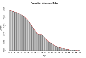
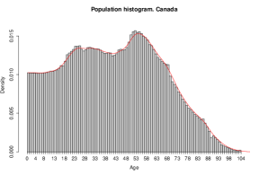
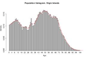
In this section we illustrate the application of trimmed $k$-barycenters in Wasserstein space to clustering age distributions of countries in the Americas. Our dataset has been downloaded (13/08/2015) from http://www.census.gov, which provides population estimates with real-time updates. This database has been used in [20] for illustration of functional PCA of densities and in [9] to show different PCA techniques, including geodesic PCA in Wasserstein space. We have excluded very small countries from our analysis and considered the 36 countries with population at least 100000. After some preprocessing (see [6] for details) for each country in the study our dataset consists of the total population numbers by age, with age ranging from 0 to 104. From this we compute an approximation to the sample quantile function for each country, which is all the information required by our methods. In Figure 1 we include three (pre-processed) population histograms. Although our computations involve only quantile functions we have added a kernel density estimate and this is what we show in subsequent figures in this section.

Figure 1: Histograms of some populations.

Our goal is to obtain a simple, but comprehensive enough description of the types of age distributions of the countries in the dataset, a task that we carry out by looking for a (small) number of age distributions that play the role of ‘main profiles’ of ‘representative types’. In the case of multivariate data this is often done with the aid of clustering techniques (see e.g. Flury [24] for an example). Here we will use trimmed $k$-barycenters for clustering this dataset of distributions. Since we are just interested in the different age-distribution profiles we will assume equal weights for all countries. In our analysis we will deal simultaneously with the choice of the number of centers, $k$, needed for a succesful summary of the profiles and of the number of outliers. Intuitively, if one distribution represents a true sector of the population, increasing the level of trimming should not lead to sharp changes of the center of this sector. In contrast, if a cluster were artificial it would consist of points belonging to different true clusters and the trimming process would result in a greater displacement of the barycenter. Also, if a point $x$ is an outlier, it should be separated from the true clusters and, once the points in the dataset which are more outlying than $x$ have been trimmed, $x$ himself should be trimmed for every reasonable choice $k$. Thus, if $x$ is really an outlier, there should exist a trimming threshold $\alpha_{0}$ such that $x$ should be trimmed in the $\alpha$-trimmed $k$-barycenter problem for $\alpha>\alpha_{0}$, independently of $k$, and if $k$-barycenters are to give a good description the dataset then the $k$ barycenters should not change much with small changes of the trimming level.

We have used the algorithm introduced in Section 3 with $\alpha\in\{\frac{1}{36},\ldots,\frac{6}{36}\}$ and $k=2,\ldots,6$. Table 1 reports the total number of times that countries were trimmed (if any) in the process. Note that for each $\alpha$ there are 5 choices of $k$, hence, the maximum number times that a country can be trimmed is 30.

Country	# of times	Country	# of times
Virgin Islands	28	Canada	22
Argentina	7	Nicaragua	7
Trinidad and Tobago	7	Uruguay	6
Jamaica	5	Guatemala	4
Belize	3	Haiti	3
Honduras	3	St Vincent & Grenadines	3
Puerto Rico	2	Grenade	2
Bolivia	1	Chile	1
Saint Lucia	1

Table 1: Number of removals from analysis, by country

For $\alpha=1/36$, the trimmed countries were Virgin Islands (V.I.), four times, and Argentina (once). For $\alpha=2/36$ only Canada and V.I. were trimmed (five times each). With $\alpha=3/36$, apart of Canada and V.I. (5 times each), Argentina (twice), Guatemala, Nicaragua and Trinidad and Tobago (T.T.) were also trimmed. At level $\alpha=4/36$ Canada and V.I. were trimmed (four times each), Argentina and Nicaragua were trimmed twice and there were eight countries trimmed once. For $\alpha=5/36$, V.I. was trimmed five times; Canada four; Jamaica, Nicaragua, T.T. and Uruguay twice and there were 8 countries trimmed only once. Finally, for $\alpha=6/36$, V.I. was trimmed five times and Canada four; T.T. and Uruguay were trimmed three times and Jamaica and Nicaragua were trimmed twice. 11 countries were trimmed once. From this table we see that the age distributions of V.I. and Canada deviate from the distributions of all the other countries and should be trimmed. The next candidates for trimming are Argentina, Nicaragua and T.T. However, for $\alpha\in\{3/36,\ldots,6/36\}$ these countries are trimmed only one third of times and we, therefore, decided to trim only two countries, that is, choose $\alpha=2/36$.

Turning to the choice of $k$, we would accept that there exist at least $k$ groups in our dataset if the variation of the $k$ barycenters, when $\alpha$ changes is small.

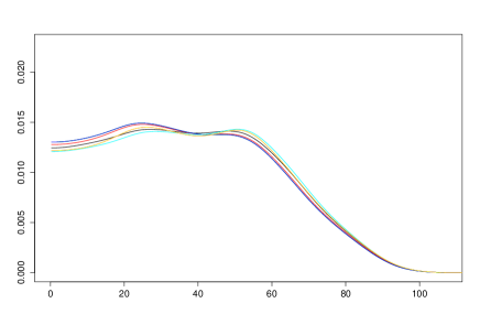
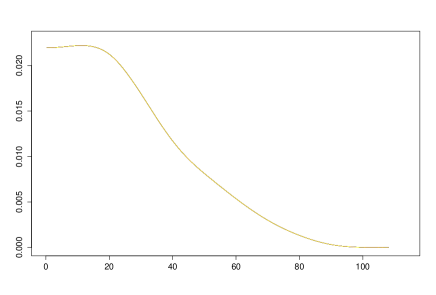
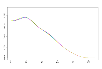
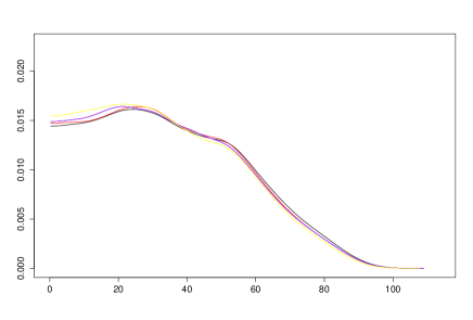
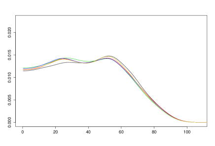
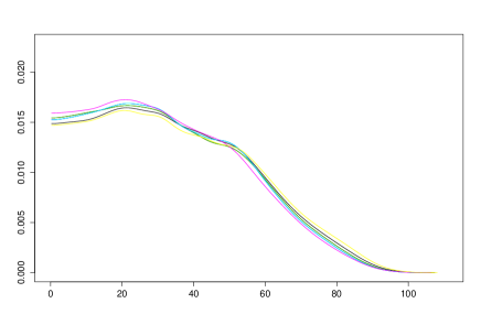
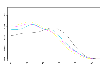
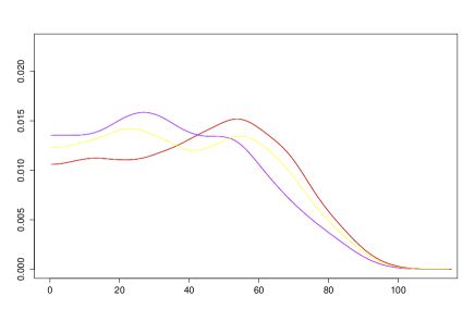
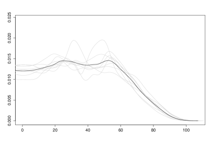
For $k=2$, letting $\alpha=0,1/36,\ldots,6/36$, we obtain seven pairs of 2-barycenters. We have grouped them by similarity. This is shown in Figure 2. Each graph includes seven barycenters, corresponding to the different trimming levels and stability becomes apparent. We conclude that $k\geq 2$. The cases $k=3$ and $k=4$ produce similar ouputs. We only comment the case $k=4$. Figure 3 contains the 4-barycenters obtained for $\alpha=0,1/36,\ldots,6/36$, with younger countries represented in the upper left corner, moving to older countries as we move left to right and from the first to the second row. We notice the very small variation among profiles in each group (in particular, there is no variation at all in the young countries group) and we conclude that $k\geq 4$. The picture changes if we take $k=5$ or $k=6$. In the first case, four of the five groups remain stable (an example appears in the upper left hand side graph in Figure 4), but we observe a new group (see the upper right graph in Figure 4) which is not stable at all. Similarly, with $k=6$ we have two unstable groups (bottom row in Figure 4). This suggests that $k=4$ is a good choice for this dataset.

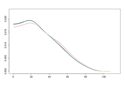
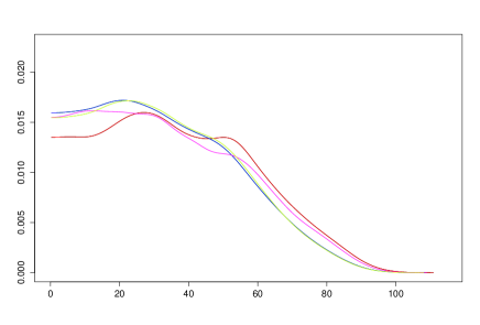
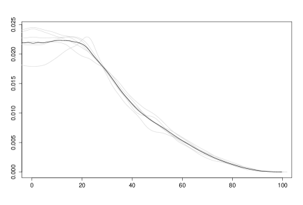
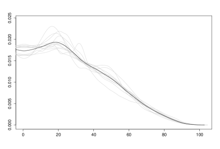
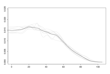
As a final summary, for the choice $\alpha=2/36$ and $k=4$ the composition of the clusters is shown in Table 2, while Figure 5 shows the density functions of the four barycenters, and those of the countries included in each group (groups I and II in top row, III and IV in bottom). We recall that trimmed countries are shown in Figure 1.

Figure 2: $2$-barycenters when $\alpha=0,1/36,\ldots,6/36$. Colors refer to different values of $\alpha$

Figure 3: $4$-barycenters when $\alpha=0,1/36,\ldots,6/36$. Colors refer to different values of $\alpha$

Figure 4: Two $5$-barycenters (resp. $6$ barycenters), first (resp. second) row, when $\alpha=0,1/36,\ldots,6/36$. Colors refer to different values of $\alpha$

Group I	Belize, Bolivia, Guatemala, Haiti, Honduras, Nicaragua
Group II	Colombia, Dominican Republic, Ecuador, El Salvador, Guyana, Jamaica,
	Mexico, Panama, Paraguay, Peru, Suriname, Venezuela
Group II	Argentina, Bahamas, Brazil , Chile, Costa Rica, Grenada, St Lucia,
	St Vincent and Grenadines
Group IV	Aruba, Barbados, Cuba, Curacao, Puerto Rico, Trinidad and Tobago,
	United States, Uruguay
Trimmed	Canada, Virgin Islands

Table 2: Barycenters and members of the groups. $k=4$ and $\alpha=2/36$

Figure 5: The $4$-barycenters (black curves) and the countries associated to each of them (grey curves)

5 Clustering aggregation in location-scatter

We present now some applications of trimmed $k$-barycenters in Wasserstein space in the aggregation of model based clustering. It is widely known that the success of a model-based clustering procedure depends strongly on the number, $k$, of ‘clusters’ (underlying distributions) and the degree of separation among them, the dimension of the space, $d$, and the sample size. Our proposal can be used with any model-based clustering statistical engine. We emphasize that our goal here is not to provide arguments for or against any particular statistical engine, but, rather, to present applications showing the positive effects that the trimmed $k$-barycenter approach can provide.

Our choice for the statistical engine in this section is TCLUST (see [29] and [25] for details). It is a consistent procedure that applied to a sample of $d$- dimensional data yields clusters obtained from estimates of centers and shapes of the clusters based on ellipsoidal regions. It involves the maximization of a pseudo-likelihood function through a natural generalization of the spurious-outlier model introduced in [26]. It is based on $k$ Gaussian distributions, allowing different scatter matrices, and assumes the presence of some underlying positive weights associated to the distributions generating the set of ‘regular’ Gaussian observations. Additionally, to avoid degeneration of solutions, TCLUST includes contraints on the eigenvalues of the covariance matrices to control the relative shapes of the clusters. For a given trimming level $\alpha$, the method discards the proportion $\alpha$ of data consisting of points with a worse fit to the model and reports the $k$ normal distributions (determined by their mean vectors, covariance matrices and associated weights) that best summarize the remaining data. We recall that the aggregation of the involved weights will be carried through (12).

We will measure the deviation between outputs of the TCLUST algorithm in terms of

$$D^{2}(\{P_{1},\dots,P_{k}\},\{Q_{1},\dots,Q_{k}\})=\min_{\sigma}\Big{\{}\frac{1}{k}\sum_{j=1}^{k}\mathcal{W}_{2}^{2}(P_{j},Q_{\sigma(j)})\Big{\}},$$ (17)

where $\sigma$ ranges in the set of permutations of $\{1,\dots,k\}$. We note that when $A_{n}$, $A\subset\mbox{$\mathcal{P}_{2}(\mathbb{R}^{d})$}$ are subsets with $k$ elements $d_{H}(A_{n},A)\to 0$ if and only if $D(A_{n},A)\to 0$, but $D$ seems more appropriate from a computational point of view.

5.1 Parallelization

In this setup we compare the performance of TCLUST applied to a large sample versus that obtained when we apply trimmed $k$-barycenters to the set of $m$ solutions obtained by TCLUST from $m$ subsamples produced through a partition of the sample.

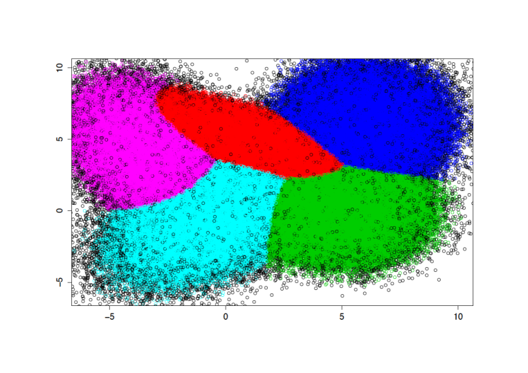
Figure 6 shows the output of TCLUST with $k=5$ and trimming level $\gamma=0.05$ on a simulated sample of size $n=10^{6}$. This sample has been obtained from 5 normal distributions $N_{i},i=1,\dots,5$ with respective proportions of the data 15%, 15%, 15%, 20% and 33% and parameters:

$$m_{1}=(0,0),\Sigma_{1}=(4,2,2,4),m_{2}=(-3,4),\Sigma_{2}=(2,-1,-1,4),m_{3}=(6,6),$$

$$\Sigma_{3}=(2,0,0,3),m_{4}=(5,0),\Sigma_{4}=(2,0,0,2),m_{5}=(1,5),\Sigma_{5}=(2,-1,-1,1).$$ (18)

The remaining 2%, to be considered merely as noise, has been obtained from a normal distribution with parameters $m_{0}=(2,2.5)$, $\Sigma_{0}=(4,0,0,4),$ playing a troubling ‘bridge-effect’ among clusters. Additionally, to explore the effect of higher dimension, we added independent observations of a standard normal distribution to fill $8$ additional variables, completing a data set of dimension $10$. We notice that the configuration of this problem presents difficulties for TCLUST, because the underlying normal distributions present a big overlap, being better suited for a mixture model. A succesful clustering analysis requires very large sample sizes. This will allow us to stress on the usefulness of parallelized computation.

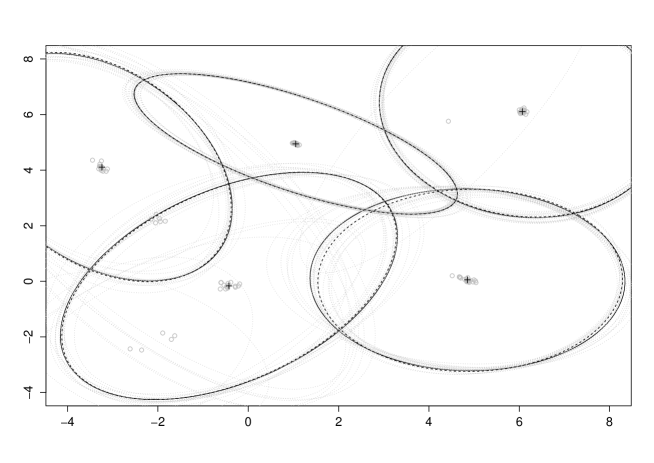
We have also applied TCLUST 100 times, with the same parameters, on the 100 subsamples of equal sizes, $10^{4}$, obtained through a partition of the large sample, thus we are just considering a parallelization of the above problem based on 100 units. To get a solution based on the ones given by the 100 units, we resort to the 0.1-trimmed $5$-barycenters. The procedure has been applied to the meta-sample of the $500=5\times 100$ provided Gaussian distributions, giving the consensus solution. The labels which relate those 5 distributions reported by the same unit have been used only to design the (non-random) initialization steps of the algorithm. This is a natural and much more efficient alternative to random initializations because we are guaranteeing that in most cases we are choosing one distribution of every detected cluster (at least by one of the units).

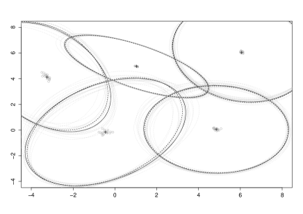
In Figure 7 we show (in gray) the ellipses corresponding to the solutions, as well as those based on the consensus solution (solid dark) and on the large sample solution (dotted dark). We note the instability of the solutions given by TCLUST for the two clusters on the left, that for a very large sample has less effect, but is clear for several solutions provided for the $10^{4}$ sized problems. We must stress the role of trimming in the $k$-barycenter step, being able to discard the most outlying solutions. In this sense, we would suggest to analyze the sensibility of the final solutions against changes in the trimming level, with stability as evidence of a succesful clustering.

As Figure 7 shows, there is complete agreement between the solution obtained from the full data set and that obtained from the parallelized version (with squared distance, $D^{2}=0.00175$). It is worth to mention that the computation time in the parallelized case is considerably shorter than that for the complete sample (33m vs 2h 8m in a MacBook Pro with a 2,5 Ghz processor Intel Core i7, using the library “parallel” in R with 8 cores). Regarding the reported weights and the aggregated obtained through (12), the greatest difference was 0.0035, corresponding to the SE cluster.

Figure 6: First and second coordinates of the TCLUST classification ($k=5$, $\alpha=0.05$, nstart = 150, restr.fact = 50, iter.max = 100, equal.weights = F) applied to simulated sample of size $10^{6}$ from model (5.1) in dimension 10. Black circles represent trimmed points.

Figure 7: Gray: first two coordinates of 95% level ellipses (with their centers) of normal distributions reported by TCLUST on 100 subsamples of size $10^{4}$ (a random partition of the full sample in Figure 6); solid black: ellipses for 0.1-trimmed $5$-barycenters of the $5\times 100$ normal distributions reported by TCLUST; dotted dark: TCLUST output for the full sample

5.2 Resampling aggregation

The use of resampling methods to improve accuracy of statistical prediction begins with the seminal works by Breiman (see e.g. [11]). In the clustering setting, ‘bagged clustering’ was initiated in Leisch [35], using an aggregation of the bootstrapped solutions based on a combination of partitioning and hierarchical methods. Later, Dudoit and Fridlyand [23] introduced other variants, resorting to plurality voting or to modifications of the dissimilarity matrix to get the final cluster solution. Subagging is a term considered in Bühlmann [12] as a ‘sobriquet for subsample aggregating where subsampling is used instead of the bootstrap for the aggregation’, while ‘subragging’ is a robust version which chooses the median instead of the mean in the aggregation step. Since our aggregation procedure is based on a robustified version of the $k$-barycenter, in the spirit, the following examples could be considered also as a bragging and subragging approaches.

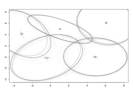
We have applied these principles to a simulated dataset generated from model (5.1), but now we consider 18 additional independent N(0,1) variables to get a data set in dimension 20. We consider a sample of size 15000 and 100 samples of size 8000 obtained by resampling in each of two scenarios: with and without replacement. Figure 8 is similar to the display in Figure 7. In each case we applied TCLUST ($k=5$, $\alpha=0.05$, nstart = 150, restr.fact = 10, iter.max = 100, equal.weights = F) to get the solution based on the full sample (dotted lines) and on 100 resamples (gray lines) of size 8000 in each case with (left) or without (right) replacement. The aggregated solutions (solid lines) are given by the trimmed $k$-barycenter procedure ($\alpha=0.1$, $k=5$) applied to the $5\times 100$ estimations.

We see in Figure 8 that subsampling looks more stable than bootstrap, but the aggregated solutions are similar by the effect of trimming. We note that the maximum difference between global and aggregated (through (12)) weights was 0.006 (resp. 0.002) for resampling with (resp. without) replacement, while the squared distances between the $k$-sets obtained between the solution obtained for the complete sample and the obtained by aggregation were respectively 0.023 and 0.012. By considering bootstrap samples (i.e. resampling with replacement and resample size equal to the original sample size), $D^{2}$ changed from 0.023 to 0.010.

Figure 8: Dotted: ellipses provided by TCLUST ($k=5$, $\alpha=0.05$, nstart = 150, restr.fact = 10, iter.max = 100, equal.weights = F) for the full dataset in subsection 5.2; Gray: 100 estimations provided by TCLUST (with the same parameters) for resamples of sizes 8000 Solid: bragging (left) and subragging (right) solutions given by the $\alpha$-trimmed $k$-barycenters procedure (for $k=5$ and $\alpha=0.1$)

5.3 Improving clustering initializations

Performance of model based clustering procedures depends on the initializations. Since most of these clustering methods involve random initializations, the number of initial random starts should be dramatically increased to get guarantee of a successful identification of the components. As we will see, our robust aggregation proposal can be also helpful in this task by combining even unfortunate solutions. We will present their effects in a simulated example which is not based on an isolated data set, but in a batch of them, which share components with common patterns. We will show how trimmed $k$-barycenters could provide smart initial solutions to clustering procedures, allowing to increase the number of well-identified populations.

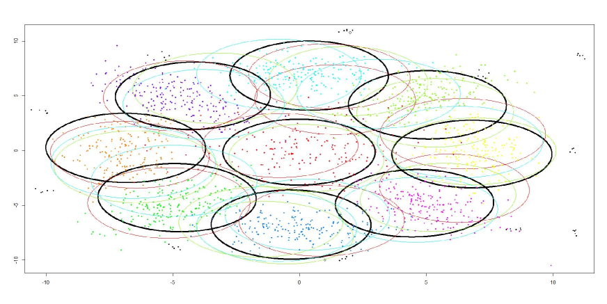
We consider 100 data sets of same sizes generated in the same way. Any data set contains 100 observations from 9 fixed normal distributions on $\mbox{$\mathbb{R}$}^{25}$. They also include a 5% of contamination data. Only the two first coordinates of the involved distributions present differences. The distribution for each observation in the other 23 variables is $N(0,I_{23})$. In Figure 9 we include the representation of a data set, where the different colors show the distributional origin of the observations. The central component is $N(0,2.25\times I_{2})$, the other main components are centered at the vertices of a regular octagon centered at the origin with radius 7. Their covariance matrices are characterized by their eigenvalues, $(\sqrt{3},\sqrt{2})$, and their eigenvectors, one corresponding to the direction joining the center and the origin and the other to its orthogonal direction. The contaminated observations correspond to data obtained from a mixture of 8 normal distributions with equal weights and covariance matrices $0.2\times I_{2}$, whose centers are uniform perturbations of the coordinates of the vertices of a regular centered octagon. For this octagon the radius is the maximum distance observed from the regular observations to the center.

The dependence of TCLUST solutions with respect to the input parameters (trimming level and restriction factor) has been studied in [30] and [31] providing evidence on stability as well as practical tools to assist in the choice of parameters. The choice of trimming level is a compromise between robustness and efficiency. It should be big enough for eliminating the effect of outliers, but not so big as to eliminate an entire cluster. For small sample sizes and high dimensions, low levels of restriction factor (controlling the relative shapes between clusters) are required for avoiding spurious solutions. These considerations lead to our choices of 0.05 for the trimming level and 4 for the restriction factor for applying TCLUST ($k=9$, $\alpha=0.05$, nstart = 50, restr.fact = 4, iter.max = 20, equal.weights = F) to each data set in this batch. After we computed the trimmed $k$-barycenters (for $k=9$) corresponding to the $9\times 100$ TCLUST estimations, for different trimming levels ranging values from 0.50 to 0.05. We find also stability with respect to the trimming level for the $k$-barycenter estimation, but, as this trimming level approaches 50% the $k$-barycenter is no longer able to find the central population and with low trimming levels the inaccuracies of TCLUST in identifying the true components are inherited by trimmed $k$-barycenter. The best performance of $k$-barycenters corresponded to trimming levels around 20%. A summary of the results is shown in Figure 9. Later we use this solution as the initial solution for TCLUST.

Figure 9: Black lines: ellipsoids of 20% trimmed $9$-barycenter of the $9\times 100$ TCLUST estimations from the 100 samples described in subsection 5.3; other colors: ellipsoids of TCLUST solutions for first 5 datasets in batch (ellipses with same color come from the TCLUST solution for the same dataset)

Now we will compare the behavior of standard TCLUST estimations based on random initial starts, with those based on the start given by the aggregation just obtained through the trimmed $k$-barycenter (kB TCLUST). For a better comparison, we also include (Oracle TCLUST) the behavior when the initial start is based just on the true parameters, a kind of oracle information not available when applying clustering in real applications. For the evaluation of these TCLUST proposals, we reutilize the batch of 100 data sets and three criteria. The first one corresponds to the overall percentage of rightly classified observations (overall %). For the second we consider the percentage of datasets in which there is a bijection between estimated clusters and real components, in the sense than more than 50% of the observations from each true component are rightly identified by the associated cluster (bijection$>50\%$). The third one is related with the overall percentage of true components, whose associated clusters identify more than the 75% of the true observations from the component (% components$>75\%$). Table 3 gives the values obtained by the mentioned proposals when applied to the batch of 100 datasets. In relation with the performance of the mentioned proposals, kB TCLUST reached a similar performance than the reference given by oracle TCLUST corresponding to right identification of the 9 components and better performance than standard TCLUST that failed in two of the 9 main populations.

	Overall	Bijection $>50\%$	% (Components $>75\%$)
kB TCLUST	86.34%	98%	88.33%
Standard TCLUST	63.10%	1%	41%
Oracle TCLUST	94.70%	100%	99.22%

Table 3: Performance comparison of TCLUST for different initial starts

5.4 Application to cytometric analysis

The automated analysis of flow cytometry data is an active field in several research areas. While traditional methods of analysis rely on subjective manual gating, in the last years, different groups have developed computational methods for identifying cell populations in multidimensional data. However, the task is by no means easy, because to the expected variability between individuals we must add noises from diverse sources. In fact, “the lack of statistical and bioinformatics tools to parallel recent high-throughput technological advancements has hindered this technology from reaching its full potential” (sic, see [37]).

Our goal here is to provide evidence of the usefulness of statistical tools, arising from the trimmed $k$-barycenters approach, in connection with this topic. We use the T cell phosphorylation dataset analyzed in Pyne et al. [41], [42] and available in the Genepattern website (http://www.broadinstitute.org/cancer/software/genepattern/FLAME-view-publish ed-data). This data set contains cytometric samples of 30 subjects in CD4, CD45RA, SLP76 and ZAP70 before (B - 13 samples) and 5 min after stimulation (A - 30 samples). There are differences in these variables for B and A samples as shown in [42], [41] and references therein. It is worth noting the recent availability of multilevel methodologies designed for simultaneous modeling and registration of cytometric data as the JCM proposal considered in [42].

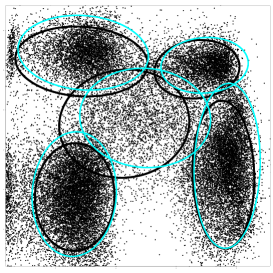
We applied trimmed $k$-baricenters (for k=5) to TCLUST estimation corresponding to each available sample in A and B sets. The three plots in Figure 10 represent observations in two samples contained in A (left and center panels) and one sample in B (right panel). It is possible appreciate in them the high variability between samples, even when they belong to the same set, as it is the case for the two samples on the left and the center panels. The plots show blue ellipsoids for representing the TCLUST estimation and black ellipsoids corresponding to the 30% trimmed $k$-barycenter based on the 30 cytometries of group A. Since the data are 4-dimensional, notice that in all the graphics in this subsection, we use the plots based on the 2 first canonical components corresponding to this trimmed $k$-barycenter and the black ellipsoids are kept as a reference.

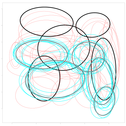
Since we have two batches of 30 (A) and 13 (B) samples, we expect that an application of trimmed $k$-barycenter with a high level of trimming (50%), allows to identify the most common pattern in the A set, which represents nearly 70% of the samples. Trimming was able to identify most of the A samples when we applied 50% trimmed $k$-barycenters to the full set of estimations provided from the samples. The procedure was able to eliminate 89.2% of samples from B, while 67.3% of samples from A survived as non-trimmed. In Figure 11, the left plot shows the trimmed k-barycenters of the B samples obtained, for $k=5$ at different levels of trimming. We should stress on the stability for most of the components estimations when using different trimming levels and the changes in the configuration of these components between A and B. The plot on the right shows the ellipsoids corresponding to 50% trimmed $k$-barycenters (gray) summarizing samples in B. The plot also includes the ellipsoids corresponding to the TCLUST solutions (non-trimmed in blue and trimmed in red).

Figure 10: Left and middle: cytometries of two individuals after stimulation (group A); right: cytometry of an individual in group B. Blue ellipsoids: TCLUST (k=5, $\alpha=0.15$, nstart=400, iter.max=50, restr.fact =25); black ellipsoids: trimmed $k$-barycenter ($k=5$, $\alpha=0.3$) based on the $30\times 5$ estimations obtained through TCLUST from the 30 cytometries of group A.

Figure 11: In the canonical coordinates of the 30% trimmed $5$-barycenters corresponding to the A samples. Left: trimmed $5$-barycenters of B samples for different trimming levels (50%, 40%, 30%, 20%, 10% and 5%; gray level ranging from black to white). Right: trimmed $5$-barycenters for both sets of estimations and trimming level $50\%$, and different estimations provided by TCLUST, in red the trimmed ones.

6 Appendix

Here we present the proofs of the main results in the paper. Most of the proofs make use of some well-known features of transportation cost metrics. For the sake of readability we include also some relevant facts concerning the $L_{2}$-Wasserstein distance defined in (3) in connection with the present work. We refer to [44] for a comprehensive approach.

We note first that the infimum in (3) is attained, that is, there exists a pair $(X,Y)$, defined on some probability space, with ${\cal L}(X)=P$ and ${\cal L}(Y)=Q$ such that $\mbox{$\mathbf{E}$}\|X-Y\|^{2}=\mathcal{W}_{2}^{2}(P,Q)$. Such a pair $(X,Y)$ is called a optimal transportation plan (o.t.p.) or optimal coupling for $(P,Q)$. If the probability $P$ has a density, the o.t.p. $(X,Y)$ for $(P,Q)$ can be represented as $(X,T(X))$ for some suitable map $T$. This optimal transport map, minimizing the transportation cost for $(P,Q)$ is the $P$-a.s. unique cyclically monotone map that transports $P$ to $Q$. Thus, optimality is a feature of the map itself and cyclically monotone maps are always optimal maps from $P$ to the image measure. As an example, an affine map, $T:\mbox{$\mathbb{R}^{d}$}\to\mbox{$\mathbb{R}^{d}$}$, written in matrix notation as $T(x)=Ax+b$, is an optimal map if and only if $A$ is a (symmetric) positive semidefinite matrix. Optimality of maps is not generally preserved by composition. However, some kind of operations like positive linear combinations and point-wise limits of optimal maps keep optimality.

For probabilities on the real line, if $F_{P}^{-1}$ and $F_{Q}^{-1}$ are the quantile functions associated to $P$ and $Q$, they are an $\mathcal{W}_{2}$-o.t.p., that is,

$$\mbox{$\mathcal{W}_{2}$}(P,Q)=\left(\int_{0}^{1}\left(F_{P}^{-1}(t)-F_{Q}^{-1}(t)\right)^{2}dt\right)^{1/2}.$$ (19)

In higher dimension there is no equivalent simple expression. However, if $m_{P},m_{Q}$ are the means of $P$ and $Q$, and $P^{*},Q^{*}$ are the corresponding centered in the mean probabilities, then we can focus on the case of centered probabilities because

$$\mbox{$\mathcal{W}_{2}^{2}$}(P,Q)=\|m_{P}-m_{Q}\|^{2}+\mbox{$\mathcal{W}_{2}^{2}$}(P^{*},Q^{*}).$$ (20)

Recall that $\mathcal{P}_{2}(\mathbb{R}^{d})$ is the set of probabilities on $\mathbb{R}^{d}$ with finite second moment. Convergence in the $\mathcal{W}_{2}$ metric on $\mathcal{P}_{2}(\mathbb{R}^{d})$, $\mbox{$\mathcal{W}_{2}$}(P_{n},P)\rightarrow 0$, is characterized by

$$P_{n}\rightarrow_{w}P\ \ \mbox{ and }\ \int_{\mbox{$\mathbb{R}^{d}$}}\|x\|^{2}P_{n}(dx)\rightarrow\int_{\mbox{$\mathbb{R}^{d}$}}\|x\|^{2}P(dx).$$ (21)

Finally, we mention that if $(P_{n})_{n},(Q_{n})_{n}$ are sequences in $\mathcal{P}_{2}(\mathbb{R}^{d})$, such that $P_{n}\rightarrow_{w}P$ and $Q_{n}\rightarrow_{w}Q$, then $\mbox{$\mathcal{W}_{2}$}(P,Q)\leq\liminf\mbox{$\mathcal{W}_{2}$}(P_{n},Q_{n})$.

A main tool for proving convergence results in the space $W_{2}(\mbox{$\mathcal{P}_{2}(\mathbb{R}^{d})$})$ (recall the definition (4) in Section 2) is given by the next couple of results, extending (21) and the subsequent comment for $\mathcal{W}_{2}$ (see e.g. Theorem 6.9 and Remark 6.12 in [44]) to the Wasserstein distance, $\mathcal{W}_{\mathcal{P}_{2}}$, defined on $W_{2}(\mbox{$\mathcal{P}_{2}(\mathbb{R}^{d})$})$ .

Theorem 6.1.

Assume $(\mu_{n})_{n},\mu\in W_{2}(\mbox{$\mathcal{P}_{2}(\mathbb{R}^{d})$})$, and consider the probability concentrated at zero, $\delta_{\{0\}}$ (that can be substituted by any other fixed probability in $\mathcal{P}_{2}(\mathbb{R}^{d})$). Convergence $\mathcal{W}_{\mathcal{P}_{2}}(\mu_{n},\mu)\rightarrow 0$ holds if and only if

$$\mu_{n}\rightarrow_{w}\mu\ \ \mbox{ and }\lim_{R\rightarrow\infty}\limsup_{n\to\infty}\int_{\mathcal{W}_{2}(\delta_{\{0\}},P)>R}\mbox{$\mathcal{W}_{2}^{2}$}(\delta_{\{0\}},P)\mu_{n}(dP)=0.$$ (22)

Proposition 6.2.

(Lower semicontinuity). If the sequences $(\mu_{n})_{n},(\nu_{n})_{n}$ in $W_{2}(\mbox{$\mathcal{P}_{2}(\mathbb{R}^{d})$})$ are such that $\mu_{n}\rightarrow_{w}\mu$ and $\nu_{n}\rightarrow_{w}\nu$, then $\mathcal{W}_{\mathcal{P}_{2}}(\mu,\nu)\leq\liminf\mathcal{W}_{\mathcal{P}_{2}}(\mu_{n},\nu_{n})$.

Now we prove the main results concerning existence and consistency of $k$-barycenters.

Theorem 6.3.

(Existence of $k-$barycenters) Let $\mu\in W_{2}(\mbox{$\mathcal{P}_{2}(\mathbb{R}^{d})$})$ and, for $k\geq 1$, define

$$V_{k}(\mu):=\inf\left\{\int\min_{i\in\{1,\dots,k\}}\mbox{$\mathcal{W}_{2}^{2}$}(P,Q_{i})\mu(dP),\{Q_{1},\dots,Q_{k}\}\subset\mbox{$\mathcal{P}_{2}(\mathbb{R}^{d})$}\right\}.$$ (23)

Then $V_{k}(\mu)\leq V_{k-1}(\mu)\leq\dots\leq V_{1}(\mu)<\infty$ and all the inequalities are strict unless $\mu$ is supported on less than $k$ elements of $\mathcal{P}_{2}(\mathbb{R}^{d})$. Moreover, there exists a $k$-barycenter of $\mu$, say ${\bf\bar{M}}=\{\bar{M}_{1},\ldots,\bar{M}_{k}\}\subset\mbox{$\mathcal{P}_{2}(\mathbb{R}^{d})$},$ that satisfies

$$\int\min_{i\in\{1,\dots,k\}}\mbox{$\mathcal{W}_{2}^{2}$}(P,\bar{M}_{i})\mu(dP)=V_{k}(\mu).$$ (24)

Proof: From the assumption $\mu\in W_{2}(\mbox{$\mathcal{P}_{2}(\mathbb{R}^{d})$})$ we see that

$$0\leq V_{k}(\mu)\leq V_{k-1}(\mu)\leq\ldots\leq V_{1}(\mu)\leq\int\mbox{$\mathcal{W}_{2}^{2}$}(P,\delta_{\{0\}})\mu(dP)<\infty.$$

Let $\{{\bf H}_{n}\}_{n}=(\{Q_{1}^{n},\ldots,Q_{k}^{n}\})_{n}$ be a minimizing sequence of $k$-sets, namely, such that

$$\int\mbox{$\mathcal{W}_{2}^{2}$}(P,{\bf H}_{n})\mu(dP)\rightarrow V_{k}(\mu).$$

We first prove that the sequence $\{{\bf H}_{n}\}_{n}$ is bounded. After a rearrangement, if necessary, we can assume that $\mathcal{W}_{2}(Q_{1}^{n},\delta_{0})\leq\cdots\leq\mathcal{W}_{2}(Q_{k}^{n},\delta_{0})$. Now, since $\mathcal{W}_{2}^{2}({\bf H}_{n},\delta_{0})\leq 2\mathcal{W}_{2}^{2}({\bf H}_{n},P)+2\mathcal{W}_{2}^{2}\mbox{$\mathcal{W}_{2}$}(P,\delta_{\{0\}})$ we see, integrating, that $\mathcal{W}_{2}^{2}({\bf H}_{n},\delta_{0})$ is a bounded sequence, that is, $\mathcal{W}_{2}^{2}(Q_{1}^{n},\delta_{0})$ is bounded, and, consequently, $\{Q_{1}^{n}\}_{n}$ is a tight sequence. Taking subsequences we can assume that for some $l\in\{2,\ldots,k\}$, $Q_{i}^{n}\to_{w}Q_{i}$, $i=1,\ldots,l$, while $\mathcal{W}_{2}^{2}(Q_{i}^{n},\delta_{0})\to\infty$ for $i\geq l+1$. By lower semicontinuity and Fatou’s Lemma we find that

$$V_{l}(\mu)\leq\int\min_{i=1,\dots,l}\mbox{$\mathcal{W}_{2}^{2}$}(P,Q_{i})\mu(dP)\leq\int\liminf_{n\to\infty}\min_{i=1,\dots,k}\mbox{$\mathcal{W}_{2}^{2}$}(P,Q_{i}^{n})\mu(dP)\leq$$

$$\liminf_{n\to\infty}\int\min_{i=1,\dots,k}\mbox{$\mathcal{W}_{2}^{2}$}(P,Q_{i}^{n})\mu(dP)=\liminf_{n\to\infty}\int\mbox{$\mathcal{W}_{2}^{2}$}(P,{\bf H}_{n})\mu(dP)=V_{k}(\mu)\leq V_{l}(\mu).$$

Therefore $\{Q_{1},\ldots,Q_{l}\}$ is a $l$-barycenter of $\mu$ and, for any choice of $\{Q_{l+1},\ldots,Q_{k}\}$, $\{Q_{1},\ldots,Q_{k}\}$ is a $k$-barycenter of $\mu$. If $\mu$ is not supported on an $l$-set then given an $l$-barycenter of $\mu$ there exists $Q_{l+1}$ and $r>0$ such that $\mathcal{W}_{2}(Q_{i},Q_{l+1})>2r$, $i=1,\ldots,l$ and $\mu(B_{\mathcal{W}_{2}}(Q_{l+1},r))>0$. But then, on the ball $B_{\mathcal{W}_{2}}(Q_{l+1},r)$, we have $\min_{i=1,\dots,l+1}\mbox{$\mathcal{W}_{2}^{2}$}(P,Q_{i})<\min_{i=1,\dots,l}\mbox{$\mathcal{W}_{2}^{2}$}(P,Q_{i})$ and, as a consequence $V_{l+1}(\mu)<V_{l}(\mu)$. $\bullet$

We note at this point that for $\mu\in W_{2}(\mbox{$\mathcal{P}_{2}(\mathbb{R}^{d})$})$ and $Q\in\mbox{$\mathcal{P}_{2}(\mathbb{R}^{d})$}$,

$$\mathcal{W}_{\mathcal{P}_{2}}^{2}(\mu,\delta_{Q})=\int\mbox{$\mathcal{W}_{2}^{2}$}(P,Q)\mu(dP).$$

In particular, for $P,Q\in\mbox{$\mathcal{P}_{2}(\mathbb{R}^{d})$}$, $\mathcal{W}_{\mathcal{P}_{2}}(\delta_{P},\delta_{Q})=\mbox{$\mathcal{W}_{2}$}(P,Q)$. We note also that the set of probabilities with support on the $k$-set $\bar{\bf Q}=\{Q_{1},\dots,Q_{k}\}$, that we will denote by $\mbox{$\mathbf{P}$}(\bar{\bf Q})$, is a closed convex set in $W_{2}(\mbox{$\mathcal{P}_{2}(\mathbb{R}^{d})$})$ and

$$\mathcal{W}^{2}_{\mathcal{P}_{2}}(\mu,\mbox{$\mathbf{P}$}(\bar{\bf Q})):=\inf\{\mathcal{W}^{2}_{\mathcal{P}_{2}}(\mu,\nu),\nu\in\mbox{$\mathbf{P}$}(\bar{\bf Q})\}=\int\min_{i=1,\dots,k}\mbox{$\mathcal{W}_{2}^{2}$}(P,Q_{i})\mu(dP).$$ (25)

In particular, when ${\bf\bar{M}}$ is a $k$-barycenter of $\mu$, this and (24) yield the characterization

$$V_{k}(\mu)=\mathcal{W}^{2}_{\mathcal{P}_{2}}(\mu,\mbox{$\mathbf{P}$}(\bar{\bf M})).$$ (26)

Theorem 6.4.

(Consistency of $k$-barycenters) Let $(\mu_{n})_{n},\mu$ be probabilities on $W_{2}(\mbox{$\mathcal{P}_{2}(\mathbb{R}^{d})$})$ such that $\mathcal{W}_{\mathcal{P}_{2}}(\mu_{n},\mu)\to 0$. Then the $k$-variations of $\mu_{n}$ converge, $V_{k}(\mu_{n})\rightarrow V_{k}(\mu)$. If $\mu$ is not supported on a $(k-1)$-set of $W_{2}(\mbox{$\mathcal{P}_{2}(\mathbb{R}^{d})$})$ and ${\bf\bar{M}}_{n}$ is any $k$-barycenter of $\mu_{n}$, the sequence $({\bf\bar{M}}_{n})_{n}$ is sequentially compact and any limit is a $k$-barycenter of $\mu$. If $\mu$ has a unique $k$-barycenter, ${\bf\bar{M}}$, then ${\bf\bar{M}}_{n}$ converges to ${\bf\bar{M}}$ in Hausdorff distance.

Proof: If ${\bf\bar{M}_{0}}$ is a $k$-barycenter of $\mu$, the convergence $\mathcal{W}_{\mathcal{P}_{2}}(\mu_{n},\mu)\to 0$ implies the convergence of the distances to the closed set $\mbox{$\mathbf{P}$}(\bar{\bf M}_{0})$, $\mathcal{W}^{2}_{\mathcal{P}_{2}}(\mu_{n},\mbox{$\mathbf{P}$}(\bar{\bf M}_{0}))\rightarrow\mathcal{W}^{2}_{\mathcal{P}_{2}}(\mu,\mbox{$\mathbf{P}$}(\bar{\bf M}_{0}))$. Hence, recall (26)

$$\int\min_{i=1,\dots,k}\mbox{$\mathcal{W}_{2}^{2}$}(P,M_{i}^{0})\mu_{n}(dP)\rightarrow\int\min_{i=1,\dots,k}\mbox{$\mathcal{W}_{2}^{2}$}(P,M_{i}^{0})\mu(dP)=V_{k}(\mu).$$ (27)

It the degenerate case of $\mu$ supported on a $(k-1)$-set, we know that $V_{k}(\mu)=V_{k-1}(\mu)=0$ and the argument leading to (27) would give $V_{k}(\mu_{n})\leq V_{k-1}(\mu_{n})\to 0$. Therefore, let us assume that $V_{k-1}(\mu)>0$ and denote by $M_{i}^{n}$, $i=1,\dots,k$ the probabilities in ${\bf\bar{M}}_{n}$. Arguing as in the proof of Theorem 6.3, the assumption $\mathcal{W}_{\mathcal{P}_{2}}(\mu_{n},\mu)\to 0$ easily leads to guarantee that the sequences $\{M_{i}^{n}\}_{n}$ are tight. Therefore, any subsequence has a subsequence (for which we keep the same notation) with weakly convergent components $M_{i}^{n}\rightarrow_{w}M_{i}$ for $i=1,\dots,k$. We write ${\bf\bar{M}}=\{M_{1},\ldots,M_{k}\}$.

On the other hand, since $\mu_{n}\rightarrow_{w}\mu$, we can apply Skorohod’s Representation Theorem (see, e.g., Theorem 11.7.2 in Dudley [22]), and assume that there are $W_{2}(\mbox{$\mathcal{P}_{2}(\mathbb{R}^{d})$})$-valued random elements $Z_{n},Z$, defined on some probability space $(\Omega,\sigma,\varUpsilon)$ with laws $\mathcal{L}(Z_{n})=\mu_{n},\mathcal{L}(Z)=\mu,$ such that $Z_{n}\rightarrow Z\ \varUpsilon-$a.s. By lower semi-continuity (Proposition 6.2), this leads to

$$\mbox{$\mathcal{W}_{2}$}(Z(\omega),M_{i})\leq\liminf_{n\to\infty}\mbox{$\mathcal{W}_{2}$}(Z_{n}(\omega),M_{i}^{n}),\ i=1,\dots,k\mbox{ for }\varUpsilon-\mbox{a. e. }\omega,$$ (28)

thus

$$\min_{i=1,\dots,k}\mbox{$\mathcal{W}_{2}$}(Z,M_{i})\leq\liminf_{n\to\infty}\min_{i=1,\dots,k}\mbox{$\mathcal{W}_{2}$}(Z_{n},M_{i}^{n})\ \varUpsilon-\mbox{ a.s..}$$ (29)

From this, Fatou’s theorem, (25) and (27) we get

$$\mathcal{W}^{2}_{\mathcal{P}_{2}}(\mu,\mbox{$\mathbf{P}$}(\bar{\bf M}))=\int\min_{i\in\{1,\dots,k\}}\mbox{$\mathcal{W}_{2}^{2}$}(P,M_{i})\mu(dP)\leq\liminf_{n\to\infty}\int\min_{i=1,\dots,k}\mbox{$\mathcal{W}_{2}$}(P,M_{i}^{n})\mu_{n}(dP)$$

$$\leq\limsup_{n\to\infty}\int\min_{i=1,\dots,k}\mbox{$\mathcal{W}_{2}$}(P,M_{i}^{n})\mu_{n}(dP)\leq\lim_{n\to\infty}\int\min_{i=1,\dots,k}\mbox{$\mathcal{W}_{2}$}(P,M_{i}^{0})\mu_{n}(dP)=V_{k}(\mu),$$ (30)

hence $V_{k}(\mu_{n})\to V_{k}(\mu)$ and any weak limit ${\bf\bar{M}}$ of a weakly convergent subsequence of ${\bf\bar{M}}_{n}$ is a $k$-barycenter of $\mu$.

It only remains to show that, in fact, these weakly convergent subsequences are convergent (through subsequences) in the $\mathcal{W}_{2}$-sense. For this, observe that inequalities in (30) are, in fact, equalities. But then (29) must be also an equality. From this, taking into account that the support of $\mu$ is not degenerated in a $(k-1)-$set and (28), we conclude that the sets $\Omega_{i}:=\left\{\omega:\mbox{$\mathcal{W}_{2}$}(Z(\omega),M_{i})=\liminf_{n\to\infty}\mbox{$\mathcal{W}_{2}$}(Z_{n}(\omega),M_{i}^{n})\right\}$ have positive probability, $\varUpsilon(\Omega_{i})>0,i=1,\dots,k.$ Choose any subsequence and take $\omega\in\Omega_{i}$ satisfying also $Z_{n}(\omega)\to Z(\omega)$. Then there exists a new subsequence for which we additionally have $\mbox{$\mathcal{W}_{2}$}(Z_{n}(\omega),M_{i}^{n})$ $\to\mbox{$\mathcal{W}_{2}$}(Z(\omega),M_{i})$. But then, by Lemma 14 in [34], $\mathcal{W}_{2}(M_{i}^{n},M_{i})\to 0$. This shows that from every subsequence we can extract a further subsequence such that $d_{H}({\bf\bar{M}}_{n},{\bf\bar{M}})\to 0$. All the other claims follow from this fact. $\bullet$

When $\mu_{n}$ are the sample distributions obtained from $n$ realizations, $P_{1},\dots,P_{n}$, of the random probability measure $\mu\in W_{2}(\mbox{$\mathcal{P}_{2}(\mathbb{R}^{d})$}),$ Varadarajan’s Theorem guarantees that $\mu_{n}\rightarrow_{w}\mu$ almost surely. Taking the probability degenerated at zero, $\delta_{\{0\}},$ the classical Strong Law of Large Numbers applied to the i.i.d. random variables $\mbox{$\mathcal{W}_{2}^{2}$}(P_{i},\delta_{\{0\}})$ states

$$\int_{\mbox{$\mathcal{P}_{2}(\mathbb{R}^{d})$}}\mbox{$\mathcal{W}_{2}^{2}$}(P,\delta_{\{0\}})\mu_{n}(dP)=\frac{1}{n}\sum_{i=1}^{n}\mbox{$\mathcal{W}_{2}^{2}$}(P_{i},\delta_{\{0\}})\rightarrow_{\mbox{a.s.}}\int_{\mbox{$\mathcal{P}_{2}(\mathbb{R}^{d})$}}\mbox{$\mathcal{W}_{2}^{2}$}(P,\delta_{\{0\}})\mu(dP),$$

hence the characterization in Theorem 6.1 of convergence in the $\mathcal{W}_{\mathcal{P}_{2}}$ sense, and Theorem 6.4, prove the Strong Law of Large Numbers for $k$-barycenters.

Theorem 6.5.

Assume that $\mu\in W_{2}(\mbox{$\mathcal{P}_{2}(\mathbb{R}^{d})$})$. If $\mu_{n}$ is the sample probability giving mass $1/n$ to the probabilities $P_{1},\ldots,P_{n}$ obtained as independent realizations of $\mu$, then $V_{k}(\mu_{n})\rightarrow V_{k}(\mu)$ a.s.. If the $k$-barycenter of $\mu$, ${\bf\bar{M}}$, is unique and ${\bf\bar{M}}_{n}$ is a sample $k$-barycenter, then the $k$-barycenters are consistent, i.e. ${\bf\bar{M}}_{n}\rightarrow_{\mbox{a.s.}}{\bf\bar{M}}$ in Hausdorff distance.

Once the existence and consistency for $k$-barycenters have been proved, the adaptation to cover the trimmed versions relies on the same arguments as those employed in Section 5.5 of [4]. Therefore we omit the proofs for Proposition 2.2 and Theorems 2.3 and 2.4. In particular it must be stressed that, in the trimmed setting, the integrability condition on the $\mu_{n}$ and $\mu$ probability measures is unnecessary. In contrast we give the following proof because it involves a different way of looking at clustering of clusters.

Proof of Theorem 2.5. We write $r=r(\eta)$ and note that $H>2$. Since

$$\bigcup_{i=1}^{k}\left(\mathbb{F}({\hat{P}}_{j})\cap B(N_{i},r)=\emptyset\right)=\Big{(}\max_{1\leq i\leq k}\min_{1\leq l\leq k}\mathcal{W}_{2}(\hat{N}_{l}^{j},N_{i})>r\Big{)}\subset\Big{(}d_{H}(\mathbb{F}(\hat{P}_{j}),\mathbb{F}({P}))>r\Big{)},$$

we see that,

$$\mbox{Pr}\left[\bigcup_{i=1}^{k}\left(\mathbb{F}({\hat{P}}_{j})\cap B(N_{i},r)=\emptyset\right)\right]\leq\mbox{Pr}\left[\mathcal{W}_{2}({\hat{P}}_{j},P)>\eta\right]<\frac{\alpha}{2},\ j=1,\dots.$$ (31)

Let us set now $X_{i}^{j}=I\{\sharp\big{(}\mathbb{F}(\mathbb{\hat{P}}_{j})\cap B(N_{i},r)\big{)}=1\}$. Observe that, for fixed $i$, $X_{1}^{1},\ldots,X_{i}^{m}$ are independent Bernoulli random variables. Call $p_{i}^{j}=\mbox{Pr}(X_{i}^{j}=1)$. The balls $B(N_{i},r)$ are pairwise disjoint (recall that $H>2$) and therefore, $\left[\bigcup_{i=1}^{k}\left(\mathbb{F}({\hat{P}}_{j})\cap B(N_{i},r)=\emptyset\right)\right]^{C}\subset(X_{i}^{j}=1)$, which implies that $p_{i}^{j}>1-\frac{\alpha}{2}$. But then, if $B_{k}$ denotes a binomial r.v. with parameters $m$ and $1-\frac{\alpha}{2},$ we see from Hoeffding’s inequality that $\mbox{Pr}\big{(}\sum_{j=1}^{m}X_{i}^{j}<m(1-\alpha)\big{)}\leq\mbox{Pr}\big{(}B_{k}<m(1-\alpha)\big{)}\leq e^{-\frac{\alpha^{2}}{2}m}$. As a consequence,

$$\mbox{Pr}\bigg{\{}\bigcup_{i=1}^{k}\bigg{[}\#\bigg{(}\bigcup_{j=1}^{m}\mathbb{F}({\hat{P}}_{j})\cap B(N_{i},r)\bigg{)}<m(1-\alpha)\bigg{]}\bigg{\}}$$

$$\leq \mbox{Pr}\big{(}\sum_{j=1}^{m}X_{i}^{j}<m(1-{\textstyle\alpha})\big{)}\leq ke^{-\frac{\alpha^{2}}{2}m}.$$

From (6) we see that, with probability at least $1-ke^{-\frac{\alpha^{2}}{2}m}$, each ball $B(N_{i},r)$ contains, at least, $m(1-\alpha)$ sample points $\hat{N}_{i}^{j}$ and, in particular, the number of points outside $\cup_{i=1}^{k}B(N_{i},r)$ is less than $\alpha km$. Hence, the optimal $\alpha$-trimmed $k$-variation is upper bounded by $r^{2}$ (take a trimming of the empirical measure concentrated on $\cup_{i=1}^{k}B(N_{i},r)$ and use the $N_{i}$’s as centers). To ease notation let us write $\mathbf{M}=\mathbf{M}_{n_{1},\ldots,n_{m};m}$ and $\hat{r}_{\alpha}$ for the associated optimal trimming radius as in Proposition 2.2. Since, by assumption, $\alpha km$ is an integer, we can assume that the optimal trimming function, $\tau_{\alpha}$ takes values in $\{0,1\}$. We write $\tilde{B}(\mathbf{M},\hat{r}_{\alpha})=\{x\in\bar{B}(\mathbf{M},\hat{r}_{\alpha}):\,\tau_{\alpha}(x)=1\}$ and similarly for $\tilde{B}(N,\hat{r}_{\alpha})$ for $N\in\mathbf{M}$. Now, the number of points outside $\tilde{B}(\mathbf{M},\hat{r}_{\alpha})$ is $\alpha km$. Hence, each ball $B(N_{i},r)$ contains, at least, $m(1-\frac{\delta}{k}-\alpha k)=m(1-(k+1)\alpha)$ points in $\tilde{B}(\mathbf{M},\hat{r}_{\alpha})$. Let us focus on the ball $B(N_{1},r)$. There exists $N\in\mathbf{M}$ such that $\tilde{B}(N,\hat{r}_{\alpha})$ contains at least a fraction $\frac{1}{k}$ of the points in $B(N_{1},r)\cap\tilde{B}(\mathbf{M},\hat{r}_{\alpha})$. But then $C:=B(N_{1},r)\cap\tilde{B}(N,\hat{r}_{\alpha})$ contains at least $\frac{m}{k}(1-(k+1)\alpha)$ points and, from equation (8), denoting $s=\mathcal{W}_{2}(N,B(N_{1},r))$ we conclude

$$r^{2}\geq\frac{1}{km(1-\alpha)}\sum_{i,j:\hat{N}_{i}^{j}\in C}{\cal W}_{2}^{2}(\hat{N}_{i}^{j},N)\geq s^{2}\frac{(1-\alpha(k+1))m}{k^{2}m(1-\alpha)}$$

and, therefore,

$$\mathcal{W}_{2}(N,B(N_{1},r))\leq rk\left(\frac{1-\alpha}{1-\alpha(k+1)}\right)^{1/2}.$$

This, in turn, implies that $\mathcal{W}_{2}(N,N_{1})\leq r\frac{H}{2}$ (recall that $H=2\big{(}1+k\big{(}\frac{1-\alpha}{1-\alpha(k+1)}\big{)}^{1/2}\big{)}$). Observe that the choice of $r$ guarantees that the balls $\bar{B}(N_{i},r\frac{H}{2})$ are disjoint. Since the choice of $N_{1}$ was arbitrary, we conclude that for every $i=1,\ldots,k$ there exists $\tilde{N}_{i}\in\mathbb{M}$ such that $W_{2}(N_{i},\tilde{N}_{i})\leq r\frac{H}{2}$. The fact that the balls $\bar{B}(N_{i},r\frac{H}{2})$ are disjoint ensures that $\{\tilde{N}_{1},\ldots,\tilde{N}_{k}\}$ is just a relabeling of $\mathbf{M}$ and, as a consequence that, with probability at least $1-ke^{-\frac{\alpha^{2}}{2}m}$,

$$d_{H}(\mathbf{M},\{N_{1},\ldots,N_{k}\})\leq\frac{rH}{2}.$$

This completes the proof. $\bullet$

Next we prove that the algorithm introduced in Section 3 converges when applied to a finite set of absolutely continuous or to discrete (with finite support) probabilities. This will be the consequence of the following propositions.

Proposition 6.6.

Let $P_{i},\ i=0,\ldots,r$ be probability measures in ${\cal P}_{2}(\mbox{$\mathbb{R}$}^{d})$ with associated weights $w_{i},\ i=0,\ldots,r$, with $\sum_{i=0}^{r}w_{i}=1.$ Let $\overline{P}$ be the barycenter of $P_{i},\ i=1,\ldots,r$ with weights $w_{i}^{*}=w_{i}(\sum_{i=1}^{r}w_{i})^{-1},\ i=1,\ldots,r$ and $\overline{P}_{0}$ be the barycenter of $P_{i},\ i=0,\ldots,r$. If we assume that $w_{0}>0$, that $P_{0}\neq\overline{P}$, and that $\overline{P}$ is absolutely continuous, then $\overline{P}_{0}\neq\overline{P}$.

Proof: Since $\overline{P}$ is absolutely continuous, there exist maps $T_{i}:\mbox{$\mathbb{R}$}^{d}\to\mbox{$\mathbb{R}$}^{d},i=0,\ldots,k$ pushing forward $\overline{P}$ to $P_{i}$, such that ${\cal W}^{2}(\overline{P},P_{i})=\int_{\mathbb{R}^{d}}\|x-T_{i}(x)\|^{2}d\overline{P}.$ Moreover, by Proposition 3.3 in [3], it must be

$${\sum_{i=1}^{r}w_{i}^{*}T_{i}(x)}=x,\ \overline{P}-\mbox{a.s.}$$

On the other hand,

$${\sum_{i=0}^{r}w_{i}T_{i}(x)}=\sum_{i=1}^{r}w_{i}x+{w_{0}}T_{0}(x)=:T^{*}(x),\ \overline{P}-\mbox{a.s.}$$

Since $T_{0}$ is not the identity $\overline{P}$-a.s., and $w_{0}>0$, it is clear that $\overline{P}\{T_{0}(x)\neq x\}>0$, and consequently (see the proof of Proposition 3.3 in [3]) we get:

$$\sum_{i=0}^{r}w_{i}{\cal W}^{2}(\overline{P},P_{i}) = \sum_{i=0}^{r}w_{i}\int\|x-T_{i}(x)\|^{2}d\overline{P}>\sum_{i=0}^{r}w_{i}\int\|T^{*}(x)-T_{i}(x)\|^{2}d\overline{P}$$

$$\geq \sum_{i=0}^{r}w_{i}{\cal W}^{2}(P_{T^{*}(x)},P_{i})\geq\sum_{i=0}^{r}w_{i}{\cal W}^{2}(\overline{P}_{0},P_{i}).\hskip 128.0374pt\bullet$$

Recall that the condition $\overline{P}$ is absolutely continuous is verified if we know that $P_{i},\ i=1,\ldots,r$ are absolutely continuous. Concerning the discrete case, let us retain the notation of the previous proposition and let $\{a^{i}_{1}\ldots,a^{i}_{h_{i}}\}$ be the support of $P_{i},i=0,1,\dots,r$. As stated in Lemma 6.7 below, $\overline{P}$ also has a finite support, say $\{b_{1},\ldots,b_{h}\}$. In this case, the optimal coupling between $\overline{P}$ and $P_{i},\ i=0,\ldots,r$, is determined by a family of positive numbers $p^{i}_{s,t},\ s=1,\ldots,h;\ t=1,\ldots,h_{i}$ which satisfy

$$\sum_{i=1}^{r}p^{i}_{s,t}=\overline{P}[b_{s}]\mbox{ and }\sum_{s=1}^{h}p^{i}_{s,t}=P_{i}[a_{t}^{i}].$$

Slight modifications of the proof of Theorem 1 in [2] lead to the following lemma.

Lemma 6.7.

With the notation above, we have that,

1. The support of $\overline{P}$ is finite.

2. For every $s=1,\ldots,h$, and $i=1,\ldots,r$, it holds: $\#\{s:p^{i}_{s,t}>0\}=1$. Moreover, if $k_{i}$ denotes the only index such that $p^{i}_{s,k_{i}}>0$, then

   $$b_{s}=\sum_{i}w_{i}^{*}a^{i}_{k_{i}},\ \mbox{ and }P_{i}[a^{i}_{k_{i}}]\geq\overline{P}[b_{s}].$$

3. There exist maps $T_{i}:\mbox{$\mathbb{R}$}^{d}\to\mbox{$\mathbb{R}$}^{d}$ such that, if the distribution of $X$ is $\overline{P}$, then the distribution of $T_{i}(X)$ is $P_{i}$ and ${\cal W}^{2}(\overline{P},P_{i})=\int_{\mathbb{R}^{d}}\|x-T_{i}(x)\|^{2}d\overline{P}.$

Item 3 in Lemma 6.7 allows to repeat the proof of Proposition 6.6 to obtain:

Proposition 6.8.

Assume the same notation as in the previous proposition, and let $P_{i},\ i=0,\ldots,r$ be probability measures with finite support. If $w_{0}>0$ and $P_{0}\neq\overline{P}$, then $\overline{P}_{0}\neq\overline{P}$.

Proposition 6.9.

Let $k\in\mbox{$\mathbb{N}$}$ fixed, and consider a family of probabilities $P_{1},\ldots,P_{r}$ with weights $w_{i}\geq 0$ and $\sum_{i}w_{i}=1$. The proposed algorithm to compute trimmed $k$-barycenters with weights converges to a local minimum of the objective function given in (13) either if the involved probabilities are absolutely continuous or if all their supports are finite.

Proof: Notice that Step 4 in the algorithm provides a partition of the set $\{1,\ldots,r\}$ in the finite family of subsets

$$T^{n} = \{i:w^{n}_{i}=0\}$$

$$R_{j}^{n} = \{i:w^{n}_{i}=1\mbox{ and }g_{i}^{n}=j\},\ j=1,\ldots,k$$

$$Q_{j}^{n} = \{i:0<w^{n}_{i}<1\mbox{ and }g_{i}^{n}=j\},\ j=1,\ldots,k.$$

Thus, $T^{n}$ contains the indices of the probabilities which are completely trimmed and $R_{j}^{n}$ those of the probabilities which are not trimmed and are associated to group $j$. After this, at most one index $i_{q}$ remains. In such a case, it belongs to one of the sets $Q_{j}^{n}$, while the remaining sets are empty. Moreover, once the two sets $\cup_{j}R_{j}^{n}$ and $T^{n}$ have been fixed, the value of $w_{i_{q}}^{n}$ is also fixed, and, then, only the index $g_{i_{q}}^{n}$ can vary. Thus, Step 4 only has a finite number of possibilities. Therefore, if we show that each time we run steps 2 and 3 the value of the objective function strictly decreases, the result will be proved because this implies that we cannot visit twice the same solution. But this is trivial because, if the probabilities are absolutely continuous, then Proposition 6.6 implies that if the stopping condition is not fulfilled, then at least a barycenter $P_{j}^{n+1}$ will vary and we will have a reduction of the objective function. The same happens using Proposition 6.8 if the supports of the probabilities are finite. $\bullet$

References

- [1] Agueh, M. and Carlier, G. (2011). Barycenters in the Wasserstein space. SIAM J. Math. Anal., 43 (2), 904–924.
- [2] Anderes, E., Borgwardt, S., and Miller, J. (2016). Discrete Wasserstein Barycenters: Optimal Transport for Discrete Data. Mathematical Methods of Operations Research, 84, 389–409.
- [3] Álvarez-Esteban, P. C., del Barrio, E., Cuesta-Albertos, J. A., and Matrán, C. (2016). A fixed-point approach to barycenters in Wasserstein space. Jour. Math. Anal. and Appl. 441(2), 744–762
- [4] Álvarez-Esteban, P. C., del Barrio, E., Cuesta-Albertos, J. A., and Matrán, C. (2016). A Wide Consensus approach to aggregation in the Wasserstein Space. Preprint.
- [5] del Barrio, E., Lescornel, H., and Loubes, J.M. (2015). A statistical analysis of a deformation model with Wasserstein barycenters: estimation procedure and goodness of fit test. Preprint. http://arxiv.org/abs/1508.06465
- [6] del Barrio, E., Cuesta-Albertos, J. A., and Matrán, C. (2016). Profiles of Pyramid Ages in American countries: A trimmed -barycenters approach. Technical Report.
- [7] Benamou, J. D., Carlier, G., Cuturi, M., Nenna, L., and Peyre, G. (2015). Iterative Bregman projections for regularized transportation problems. SIAM J. Sci. Comput., 37(2), 1111–1138.
- [8] Bigot, J. and Klein, T. (2015). Consistent estimation of a population barycenter in the Wasserstein space. ArXiv e-prints, arXiv:1212.2562v5, March 2015.
- [9] Bigot, J., Gouet, R., Klein, T., and López, A. (2013). Geodesic PCA in the Wasserstein space by Convex PCA. To appear in Ann. Inst. Henri Poincaré, Probab. Statist.
- [10] Boissard, E., Le Gouic, T. and Loubes, J-M. (2015). Distribution’s template estimate with Wasserstein metrics. Bernoulli, 21(2), 740–759.
- [11] Breiman, L. (1996) Bagging predictors. Machine Learning, 24, 123–140.
- [12] Bühlmann, P. (2012). Bagging, Boosting and Ensemble Methods. In Handbook of Computational Statistics: Concepts and Methods. Eds. Gentle, E.J., Härdle, K.W. and Mori, Y., pp. 985–1022. Springer. Berlin
- [13] Carlier, G., Oberman, A. and Oudet, E. (2015). Numerical methods for matching for teams and Wasserstein barycenters, ESAIM Math. Model. Numer.Anal., 49(6), 1621–1642.
- [14] Carlier, G., Chernozhukov, V., and Galichon, A. (2015). Vector Quantile Regression: An Optimal Transport Approach. Ann. Statist., to appear.
- [15] Chernozhukov, V., Galichon, A., Hallin, M., and Henry, M. (2014). Monge-Kantorovich Depth, Quantiles, Ranks, and Signs. Ann. Statist., to appear.
- [16] Cuesta-Albertos, J. A., Gordaliza, A., and Matrán, C. (1997). Trimmed k-means: An attempt to robustify quantizers. Ann. Statist., 25(2), 553–576.
- [17] Cuesta-Albertos, J. A., and Fraiman, R. (2007). Impartial trimmed k-means for functional data. Computational Statistics and Data Analysis, 51(10), 4864–4877.
- [18] Cuesta-Albertos, J. A. and Matrán, C. (1988) The Strong Law of Large Numbers for -means and best possible nets of Banach valued random variables. Probab. Theo. Related Fields 78, 523–534
- [19] Cuturi, M. and Doucet, A. (2014). Fast computation of Wasserstein barycenters, in Proceedings of the 31st International Conference on Machine Learning, Beijing, China, 2014. JMLR: W&CP vol 32.
- [20] Delicado, P. (2011). Dimensionality reduction when data are density functions. Computational Statistics and Data Analysis, 55(1), 401–420.
- [21] Dobric, V. and Yukich, J.E. (1995). Asymptotics for transportation cost in high dimensions. J. Theor. Probab., 8 97–118.
- [22] Dudley, R. M. (1989). Real Analysis and Probability. Wadsworth & Brooks.
- [23] Dudoit, S., and Fridlyand, J. (2003). Bagging to improve the accuracy of a clustering procedure. Bioinformatics, 19(9), 1090–1099.
- [24] Flury, B. (1993) Estimation of principal points. Appl. Statist., 42(1), 139–151
- [25] Fritz, H., García-Escudero, L. A., and Mayo-Iscar, A. (2012). tclust: An R Package for a Trimming Approach to Cluster Analysis. Journal of Statistical Software, 47(12).
- [26] Gallegos, M.T. and Ritter, G. (2005), A robust method for cluster analysis, Ann. Statist., 33, 347-380.
- [27] García-Escudero, L. A., and Gordaliza, A. (2005). A Proposal for Robust Curve Clustering. Journal of Classification, 22(2), 185–201.
- [28] García-Escudero, L. A., Gordaliza, A., and Matrán, C. (2003). Trimming Tools in Exploratory Data Analysis. Journal of Computational and Graphical Statistics, 12(2), 434–449.
- [29] García-Escudero, L. A., Gordaliza, A., Matrán, C., and Mayo-Iscar, A. (2008). A general trimming approach to robust cluster analysis. Ann. Statist., 36(3), 1324–1345.
- [30] García-Escudero, L. A., Gordaliza, A., Matrán, C., and Mayo-Iscar, A. (2011). Exploring the number of groups in robust model-based clustering. Statistics and Computing, 21, 585–599
- [31] García-Escudero, L. A., Gordaliza, A., Matrán, C., and Mayo-Iscar, A. (2015). Avoiding Spurious Local Maximizers in Mixture Modeling. Statistics and Computing 25, 619–633
- [32] Kneip, A., and Gasser, T. (1992). Statistical Tools to analyze Data Representing a Sample of Curves. Ann. Statistics, 20(3), 1266–1305.
- [33] Hennig, C; Meila, M.; Murtagh, F.; and Rocci, R. Eds. (2016). Handbook of Cluster Analysis. Chapman and Hall/CRC
- [34] Le Gouic, T. and Loubes, J.M. (2016). Existence and consistency of Wasserstein barycenters. To appear in Probab. Theo. Related Fields
- [35] Leisch, F.(1999) Bagged clustering. Technical report. http://www.ci.tuwien.ac.at/ ?leisch/papers/ fl-techrep.html
- [36] Lember, J. (2003). On minimizing sequences for k-centres. Journal of Approximation Theory, 120(1), 20–35.
- [37] Lo, K., Brinkman, R. R., and Gottardo, R. (2008). Automated gating of flow cytometry data via robust model-based clustering. Cytometry. Part A : The Journal of the International Society for Analytical Cytology, 73(4), 321 32. doi:10.1002/cyto.a.20531
- [38] Luschgy, H., and Pagès, G. (2002). Functional quantization of Gaussian processes. Journal of Functional Analysis, 196, 486–531.
- [39] Pärna, K. (1986). Strong consistency of k-means clustering criterion, Acta Comm. Univ. Tartuensis 733 86–96.
- [40] Pärna, K. (1990). On the existence and weak convergence of k-centres in Banach spaces, Acta Comm. Univ. Tartuensis 893, 17–28.
- [41] Pyne, S., Hu, X., Wang, K., et al. (2009). Automated high-dimensional flow cytometric data analysis. Proceedings of the National Academy of Sciences of the United States of America, 106(21), 8519–8524.
- [42] Pyne, S., Lee, S. X., Wang, K., Irish, J., Tamayo, P., Nazaire, M. D., … & Nolan, G. P. (2014). Joint modeling and registration of cell populations in cohorts of high-dimensional flow cytometric data. PloS one, 9(7), e100334.
- [43] Sverdrup-Thygeson, H., 1981. Strong law of large numbers for measures of central tendency and dispersion of random variables in compact metric spaces. Ann. Statist. 9 (1), 141–145.
- [44] Villani, C. (2008). Optimal Transport: Old and New, Vol. 338. Springer Science & Business Media.