1 Introduction

Motivation
Kitaev models [28] and Lewin-Wen models [33, 34], which were shown to be equivalent to Kitaev models in [14, 25], have attracted strong interest in condensed matter physics and topological quantum computing. They assign to an oriented surface $\Sigma$ a finite-dimensional vector space, the protected space, which is a topological invariant of $\Sigma$. They also exhibit topological excitations with braid group statistics, electro-magnetic duality and can be equipped with additional structures such as defects and domain walls [13, 29, 12], which are a focus of current research.

Kitaev models are also of strong interest from the perspective of topological quantum field theory as they are related to Turaev-Viro TQFTs [44, 10]. It was shown in [5, 30, 24, 25] that the protected space of a Kitaev model for a finite-dimensional semisimple Hopf algebra $H$ on an oriented surface $\Sigma$ coincides with the vector space $Z_{TV}(\Sigma)$ that the Turaev-Viro TQFT for the representation category $H$-Mod assigns to $\Sigma$. If one interprets Turaev-Viro invariants as a discretised path integrals [8, 9], Kitaev models can be viewed as their Hamiltonian counterparts. From this point of view, the linear map $Z_{TV}(M):Z_{TV}(\Sigma)\to Z_{TV}(\Sigma^{\prime})$ that the Turaev-Viro TQFT assigns to a 3-manifold with boundary $\partial M=\Sigma\coprod\bar{\Sigma}^{\prime}$ describes a transition between Kitaev models on $\Sigma$ and $\Sigma^{\prime}$.

This relation between Kitaev models and TQFTs extends to the case with excitations. Excitations in a Kitaev model for $H$ are labelled by representations of the Drinfeld double $D(H)$ and correspond to Turaev-Viro TQFTs with line defects [24, 5]. These were essential in establishing the equivalence of Turaev-Viro TQFTs for $H$-Mod and the Reshetikhin-Turaev TQFTs for $D(H)$-Mod in [6, 7, 27, 43].

The topological nature of Kitaev models and their relation to Turaev-Viro and Reshetikhin-Turaev TQFTs raises three obvious questions, which remained open despite their conceptual importance:

1. Is there a Hamiltonian analogue of Reshetikhin-Turaev TQFTs defined along the same lines as Kitaev models? If yes, can one precisely relate the Kitaev model for a Hopf algebra $H$ and the Hamiltonian analogue of a Reshetikhin-Turaev TQFT for its Drinfeld double $D(H)$?
   

2. Can a Kitaev model for a Hopf algebra $H$ be viewed as a Hopf algebra analogue of a group-valued lattice gauge theory? This is strongly suggested by the structure of Kitaev models, e. g. that they are defined in terms of a graph embedded in a surface $\Sigma$, that they exhibit symmetries at each vertex and face of the graph and that these symmetries act trivially on the protected space. It is also likely due to their relation to Reshetikhin-Turaev TQFTs, which were obtained by quantising Chern-Simons gauge theories [45, 42].
   

3. Are there classical analogues of a Kitaev models defined in terms of Poisson or symplectic structures associated with $\Sigma$? Although Kitaev models were defined ad hoc and not by quantising classical structures, this seems natural due to their interpretation as quantum models. It is also suggested by their relation to Reshetikhin-Turaev TQFTs, which quantise Chern-Simons gauge theories and hence moduli spaces of flat connections on $\Sigma$.

Main results
The article addresses these three questions. More specifically, we show that the algebra of operators that act on the protected space of a Kitaev model is isomorphic to the quantum moduli algebra obtained in the combinatorial quantisation of Chern-Simons gauge theory by Alekseev, Grosse and Schomerus [1, 3] and by Buffenoir and Roche [17, 18]. The protected space of a Kitaev model for a finite-dimensional semisimple Hopf algebra $H$ is therefore given as a representation space of the quantum moduli algebra for its Drinfeld double $D(H)$. This establishes a complete equivalence between the Kitaev models and the combinatorial quantisation of Chern-Simons theory and shows that Kitaev models are not a new class of models but a special case of the older and more general models in [1, 2, 3, 17, 18].

Moreover, it was shown in [18, 3] that the quantum moduli algebra can be viewed as the Hamiltonian analogue of a Reshetikhin-Turaev TQFT. Its representation spaces coincide with the vector spaces $Z_{RT}(\Sigma)$ that the Reshetikhin-Turaev TQFT assigns to $\Sigma$, and both give rise to the same action of the mapping class group $\mathrm{Map}(\Sigma)$. This addresses the first question and establishes a relation $(*)$ between Kitaev model for $H$ and the combinatorial model for $D(H)$ that is analogous to the relation between a Turaev-Viro TQFT for the representation category $H$-Mod and the Reshetikhin-Turaev TQFT for the representation category $D(H)$-Mod from [6, 7, 27, 43]:

As the quantum moduli algebra was obtained in [17, 1] by canonically quantising the symplectic structure on the moduli space of flat connections on $\Sigma$ from [23, 4], this also addresses the third question about the corresponding Poisson and symplectic structures. Moreover, all structures that describe the relation between the two models have Poisson analogues in the theory of Poisson-Lie groups. Although this aspect is not developed further here, this defines Poisson analogues of Kitaev models and relates them to symplectic structures on moduli spaces of flat connections on surfaces.

Finally, it was shown in [38] that the combinatorial model [1, 2, 3, 17, 18] can be derived from a set of simple axioms that generalise group valued lattice gauge theories to ribbon Hopf algebras. These axioms encode minimal physics requirements for a local lattice gauge theory and imply that the relevant mathematical structures are module algebras over Hopf algebras. In this sense, the combinatorial model is a generalisation of the notion of a lattice gauge theory from a group to a ribbon Hopf algebra. The equivalence of Kitaev models to combinatorial models shows that the former can indeed be interpreted as a Hopf algebra valued lattice gauge theory.

This viewpoint is also essential in establishing the correspondence between the two models. Many of the results in [28, 15] and in [1, 2, 3, 17, 18] are formulated in terms of matrix elements in irreducible representations. While this presents certain computational advantages within the models, it becomes an obstacle when relating them. The more algebraic and basis independent formulation in terms of a Hopf algebra gauge theory in [38] allows one to relate the models in a simpler and more conceptual way.

Detailed description of results
In this article we consider Kitaev models for a finite-dimensional semisimple Hopf algebra $H$, as introduced in [15], and the combinatorial model for the Drinfeld double $D(H)$ from [1, 2, 17], in its formulation as a Hopf algebra gauge theory [38]. Besides the Hopf algebras $H$ and $D(H)$ the input data in both models is a ribbon graph $\Gamma$, a directed graph with a cyclic ordering of the edge ends at each vertex. The relation between the two models is obtained by thickening $\Gamma$ to a ribbon graph ${\Gamma_{D}}$ in which each edge of $\Gamma$ is replaced by a rectangle and each vertex of $\Gamma$ by a polygon. While the Hopf algebra gauge theory is associated with the ribbon graph $\Gamma$, the natural setting for the Kitaev model is the thickened graph ${\Gamma_{D}}$.

The concept that is fundamental in relating the two models is holonomy, which we define as a functor from the path groupoid of $\Gamma$ or ${\Gamma_{D}}$ into a category constructed from the Hopf algebra data. For ribbon paths these holonomies yield Kitaev’s ribbon operators [28]. However, our notion of holonomy is more general and defined for any path in ${\Gamma_{D}}$, not only ribbon paths. This is essential in relating the two models. By selecting an adjacent face at each vertex - a site in the language of Kitaev models or a cilium in the language of Hopf algebra gauge theory - we associate to each oriented edge $e\in E$ the following two paths $p_{e,\pm}$ in ${\Gamma_{D}}$.

The holonomies of the paths $p_{e,\pm}$, which are not ribbon paths in the sense of [28, 13, 15], coincide. By sending the holonomy of an edge $e$ of $\Gamma$ to the holonomies of the paths $p_{e,\pm}$ in ${\Gamma_{D}}$, we then obtain an explicit relation between the algebraic structures in a Hopf algebra gauge theory and in the Kitaev models. This relation involves three layers:

$\bullet$ The algebra of functions and the algebra of triangle operators: The algebra $\mathcal{A}^{*}_{\Gamma}$ of functions in a Hopf algebra gauge theory for $D(H)$ is the vector space $D(H)^{*\otimes E}$ obtained by associating a copy of the dual Hopf algebra $D(H)^{*}$ to each edge of $\Gamma$. However, its algebra structure is not the canonical one from the tensor product, but deformed at each vertex by the universal $R$-matrix of $D(H)$. The corresponding structure in the Kitaev model for $H$ is the algebra generated by the triangle operators $L^{h}_{e,\pm}$ and $T^{\alpha}_{e,\pm}$ for each each edge $e$ of $\Gamma$ and indexed by elements $h\in H$ and $\alpha\in H^{*}$. These triangle operators act on the vector space $H^{\otimes E}$ via the left and right regular action of $H$ and $H^{*}$ on $H$. They form an algebra isomorphic to the $E$-fold tensor product $\mathcal{H}(H)^{\otimes E}$ of the Heisenberg double of $H$. The first central result is that under certain assumptions on $\Gamma$ these two algebras are isomorphic (Theorems 7.3 and 7.6):

Theorem.

Let $\Gamma$ be a regular ribbon graph. Then the holonomies of the paths $p_{e,\pm}$ induce an algebra isomorphism $\chi:\mathcal{A}^{*}_{\Gamma}\to\mathcal{H}(H)^{op\otimes E}$ from the algebra of functions $\mathcal{A}^{*}_{\Gamma}$ of a Hopf algebra gauge theory for $D(H)$ to the algebra formed by the triangle operators in the Kitaev model for $H$.

$\bullet$ Gauge symmetries: The second layer of correspondence concerns the gauge symmetries of the two models. Gauge transformations in the Hopf algebra gauge theory are obtained by associating a copy of the Drinfeld double $D(H)$ to each vertex of $\Gamma$ and are given by the Hopf algebra $D(H)^{\otimes V}$. The algebra $\mathcal{A}^{*}_{\Gamma}$ of functions is a module algebra over this Hopf algebra. Consequently, the submodule of invariants is a subalgebra $\mathcal{A}^{*}_{\Gamma\,inv}\subset\mathcal{A}^{*}_{\Gamma}$, the subalgebra of gauge invariant observables.

These gauge symmetries correspond to the symmetries associated with the vertex and face operators in the Kitaev models. These operators are given as the holonomies of paths in ${\Gamma_{D}}$ that go clockwise around the vertices and faces of $\Gamma$. For each site of $\Gamma$, they define a faithful representation of the Drinfeld double $D(H)$. Our second main result in Theorem 8.1 states that these representations give the algebra of triangle operators the structure of a module algebra over the Hopf algebra $D(H)^{\otimes V}$. Moreover, we find that the algebra isomorphism that relates it to the algebra of functions in a Hopf algebra gauge theory is compatible with these gauge symmetries:

Theorem.

For each regular ribbon graph $\Gamma$, the vertex and face operators equip the algebra $\mathcal{H}(H)^{op\otimes E}$ of triangle operators with the structure of a $D(H)^{\otimes V}$-right module algebra. The algebra isomorphism $\chi:\mathcal{A}^{*}_{\Gamma}\to\mathcal{H}(H)^{op\otimes E}$ is a module morphism and induces an algebra isomorphism between the subalgebras of invariants $\mathcal{A}^{*}_{\Gamma\,inv}\subset\mathcal{A}^{*}_{\Gamma}$ and $\mathcal{H}(H)^{op\otimes E}_{inv}\subset\mathcal{H}(H)^{op\otimes E}$.

$\bullet$ Curvature: The third layer of correspondence between Kitaev models and Hopf algebra gauge theories concerns curvatures, which are the holonomies of the faces of $\Gamma$ and ${\Gamma_{D}}$. In the Hopf algebra gauge theory, the holonomies of the faces of $\Gamma$ give rise to an algebra morphism from the character algebra or the centre of $D(H)$ into the centre $Z(\mathcal{A}^{*}_{\Gamma\,inv})$ of the algebra of gauge invariant observables. By taking the product of these holonomies over all faces of $\Gamma$ and inserting the Haar integral of $D(H)$, one obtains a projector on the quantum moduli algebra $\mathcal{M}_{\Gamma}$.

As the faces of the thickened graph ${\Gamma_{D}}$ correspond to either faces, vertices or edges of $\Gamma$ and the holonomies of the latter are trivial, curvatures in Kitaev models are given by the vertex and face operators. By taking the product of these holonomies for all vertices and faces of $\Gamma$ and inserting the Haar integrals of the Hopf algebras $H$ and $H^{*}$ one obtains Kitaev’s Hamiltonian $H_{\mathrm{K}}$, which is a projector from $H^{\otimes E}$ on the protected space.

We show that the Hamiltonian defines a projector on a subalgebra $\mathcal{H}(H)^{\otimes E}_{flat}\subset\mathcal{H}(H)^{\otimes E}_{inv}$, which consists of those elements that satisfy the relation $H_{\mathrm{K}}\cdot X\cdot H_{\mathrm{K}}=X$. This is the subalgebra of operators that act on the protected space. We then prove that for each site of $\Gamma$ the algebra isomorphism $\chi$ sends the holonomy of the associated face in $\Gamma$ to the product of the associated vertex and face operator of the Kitaev model. This leads to our third main result in Theorem 8.3:

Theorem.

For each regular ribbon graph $\Gamma$, the algebra isomorphism $\chi:\mathcal{A}^{*}_{\Gamma}\to\mathcal{H}(H)^{op\otimes E}$ induces an algebra isomorphism $\chi:\mathcal{M}_{\Gamma}\to\mathcal{H}(H)^{op\otimes E}_{flat}$.

Both, the quantum moduli algebra $\mathcal{M}_{\Gamma}$ and Kitaev’s protected space were shown to be topological invariants [28, 15, 1, 2, 17, 38]. They depend only on the homeomorphism class of the oriented surface obtained by gluing discs to the faces of $\Gamma$. As the same holds for the algebra $\mathcal{H}(H)^{\otimes E}_{flat}$ this theorem establishes a precise equivalence between the topological invariants of the Kitaev model for $H$ and the Hopf algebra gauge theory for $D(H)$.

This equivalence between Kitaev models and Hopf algebra gauge theory also has a geometrical interpretation. The thickened ribbon graph ${\Gamma_{D}}$ for the Kitaev model can be viewed as a ‘graph double’ of the ribbon graph $\gamma$, because it combines the ribbon graph $\Gamma$ with its Poincaré dual $\bar{\Gamma}$. In Kitaev models Poincaré duality corresponds to Hopf algebra duality: The edges of ${\Gamma_{D}}$ associated with edges of $\Gamma$ carry the triangle operators $T^{\alpha}_{e,\pm}$ indexed by elements $\alpha\in H^{*}$. The edges of ${\Gamma_{D}}$ associated with edges of $\bar{\Gamma}$ carry the triangle operators $L^{h}_{e,\pm}$ indexed by elements $h\in H$. This allows one to view the Kitaev model for the Hopf algebra $H$ as a factorisation of the Hopf algebra gauge theory for the Drinfeld double $D(H)$, in which gauge fields on $\Gamma$ with values in $D(H)$ are factorised into gauge fields on $\Gamma$ and on $\bar{\Gamma}$ with values in $H\subset D(H)$ and $H^{*}\subset D(H)$. Similarly, the $D(H)$-valued gauge transformations and curvatures in the Hopf algebra gauge theory factorise into gauge transformations and curvatures on $\Gamma$ and on $\bar{\Gamma}$ with values in $H\subset D(H)$ and $H^{*}\subset D(H)$. The former are associated with vertex and the latter with face operators.

Structure of the article: In Section 2 we introduce the relevant notation, the background on Hopf algebras and the graph theoretical background needed in the article. Section 3 contains a brief summary of Kitaev models, and Section 4 summarises the background on combinatorial quantisation and Hopf algebra gauge theory. In Section 5 we introduce a generalised notion of holonomy for Kitaev models, investigate its algebraic properties and show that it reduces to the ribbon operators for ribbon paths. In particular, this applies to the holonomies of paths around the vertices and faces of $\Gamma$, which define the vertex and face operators of the Kitaev model.

In Section 6 we show that Kitaev models exhibit the mathematical structures of a Hopf algebra gauge theory. We prove that the vertex and face operators give the algebra of triangle operators the structure of a right module algebra over a Hopf algebra of gauge transformations and investigate its subalgebra of invariants. We show that the Hamiltonian of the Kitaev model arises from the curvatures of the faces of ${\Gamma_{D}}$ and projects on a subalgebra of operators on the protected space.

Sections 7 and 8 contain the core results of the article. In Section 7 we prove that under certain assumptions on $\Gamma$ the holonomies of the paths $p_{e,\pm}$ in ${\Gamma_{D}}$ induce an algebra isomorphism between the algebra of functions of a Hopf algebra gauge theory and Kitaev’s triangle operator algebra. In Section 8 we show that this algebra isomorphism is a morphism of module algebras and hence induces an isomorphism between their subalgebras of invariants. We then establish that this algebra isomorphism relates the curvatures of the two models and prove that it induces an isomorphism between the quantum moduli algebra and the algebra of operators acting on the protected space.

2 Background

2.1 Notations and conventions

Throughout the article $\mathbb{F}$ is a field of characteristic zero. For an algebra $A$ and $n\in\mathbb{N}$ we denote by $A^{\otimes n}$ the $n$-fold tensor product of $A$ with itself, always taken over $\mathbb{F}$ unless specified otherwise. If $X$ is a finite set of cardinality $|X|$, we write $A^{\otimes X}$ instead of $A^{\otimes|X|}$ and denote by $\tau:\Pi_{X}A\to A^{\otimes X}$ the canonical $|X|$-linear surjection. Identifying $\Pi_{X}A$ with the vector space of maps $f:X\to A$, we define $a_{x}:X\to A$ for $x\in X$ and $a\in A$ as the map with $a_{x}(x)=a$ and $a_{x}(y)=1$ for $y\neq x$ and denote by $(a)_{x}=\tau(a_{x})$ the associated element in $A^{\otimes X}$. This corresponds is the pure tensor in $A^{\otimes X}$ that has entry $a$ in the copy of $A$ associated with $x\in X$ and $1$ in all other entries.

Similarly, for $a^{1},...,a^{n}\in A$ and pairwise distinct $x_{1},...,x_{n}\in X$, we define $(a^{1}\otimes...\otimes a^{n})_{x_{1},...,x_{n}}$ as the pure tensor in $A^{\otimes X}$ that has entry $a^{1}$ in the copy of $A$ in $A^{\otimes X}$ associated with $x_{1}$, $a^{2}$ in the copy associated with $x_{2}$ etc. It is given by $(a^{1}\otimes...\otimes a^{n})_{x_{1}...x_{n}}:=\tau((a^{1},...,a^{n})_{x_{1},...,x_{n}})$, where $(a^{1},...,a^{n})_{x_{1}...x_{n}}:=(a^{1})_{x_{1}}\cdot(a^{2})_{x_{2}}\cdots(a^{n})_{x_{n}}:X\to A$ and the product is taken with respect to the pointwise multiplication in $A$. We denote by $\iota_{x_{1}...x_{k}}:A^{\otimes n}\to A^{\otimes X}$, $a^{1}\otimes...\otimes a^{n}\mapsto(a^{1}\otimes...\otimes a^{n})_{x_{1},...,x_{n}}$ the associated inclusion maps. For linear maps $f_{1},...,f_{n}:A\to A$ we define the linear map $(f_{1}\otimes...\otimes f_{n})_{x_{1}...x_{n}}:A^{\otimes X}\to A^{\otimes X}$ by $(f_{1}\otimes...\otimes f_{n})_{x_{1},...,x_{n}}((a)_{x_{i}})=(f_{i}(a))_{x_{i}}$ for all $i\in\{1,...,n\}$ and $(f_{1}\otimes...\otimes f_{n})_{x_{1},...,x_{n}}((a)_{y})=(a)_{y}$ for $y\notin\{x_{1},...,x_{n}\}$.

For Hopf algebras we use Sweedler notation without summation signs. We write $\Delta(h)={h}_{({1})}\otimes{h}_{({2})}$ for the comultiplication $\Delta:H\to H\otimes H$ of a Hopf algebra $H$ and also use this notation for elements of $H\otimes H$, e. g. $R={R}_{({1})}\otimes{R}_{({2})}$ for a universal $R$-matrix. We denote by $H^{op}$ and $H^{cop}$, respectively, the Hopf algebra with the opposite multiplication and comultiplication and by $H^{*}$ the dual Hopf algebra. Unless specified otherwise, we use Latin letters for elements of $H$ and Greek letters for elements of $H^{*}$. The pairing between $H$ and $H^{*}$ is denoted $\langle\;,\;\rangle:H^{*}\otimes H\to\mathbb{F}$, $\alpha\otimes h\mapsto\alpha(h)$, and the same notation is used for the induced pairing $\langle\,,\,\rangle:H^{*\otimes n}\otimes H^{\otimes n}\to\mathbb{F}$.

2.2 Hopf algebras

In this subsection we summarise basic facts about Hopf algebras. Unless specific citations are given, the results can be found in textbooks on Hopf algebras, such as [26, 36, 39, 41].

Theorem 2.1 ([20]).

Let $H$ be a finite-dimensional Hopf algebra. Then there exists a unique quasitriangular Hopf algebra structure on $H^{*}\otimes H$ for which $H\cong 1\otimes H$ and $H^{*cop}\cong H^{*cop}\otimes 1$ are Hopf subalgebras. In terms of a basis $\{x_{i}\}$ of $H$ and the dual basis $\{\alpha^{i}\}$ of $H^{*}$, it is given by

$$(\alpha\otimes h)\cdot(\alpha^{\prime}\otimes h^{\prime})=\langle\alpha^{\prime}_{(3)},h_{(1)}\rangle\langle S^{-1}(\alpha^{\prime}_{(1)}),h_{(3)}\rangle\,\alpha\alpha^{\prime}_{(2)}\otimes h_{(2)}h^{\prime} 1=1_{H^{*}}\otimes 1_{H}$$ (1)

$$\Delta(\alpha\otimes h)=\alpha_{(2)}\otimes h_{(1)}\otimes\alpha_{(1)}\otimes h_{(2)} \epsilon(\alpha\otimes h)=\epsilon(\alpha)\epsilon(h)$$

$$S(\alpha\otimes h)=\langle{\alpha}_{({1})},{h}_{({3})}\rangle\langle S^{-1}({\alpha}_{({3})}),{h}_{({1})}\rangle\;S({\alpha}_{({2})})\otimes S({h}_{({2})}) R=\Sigma_{i}\,1\otimes x_{i}\otimes\alpha^{i}\otimes 1.$$

This Hopf algebra is called the Drinfeld double of $H$ and denoted $D(H)$.

Remark 2.2.

If $\{x_{i}\}$ a basis of $H$ and $\{\alpha^{i}\}$ the dual basis of $H^{*}$, the dual Hopf algebra $D(H)^{*}$ of the Drinfeld double $D(H)$ is the vector space $H\otimes H^{*}$ with the following Hopf algebra structure

$$(y\otimes\gamma)\cdot(z\otimes\delta)=zy\otimes\gamma\delta 1=1_{H}\otimes 1_{H^{*}}$$ (2)

$$\Delta(y\otimes\gamma)=\Sigma_{i,j}\;{y}_{({1})}\otimes\alpha^{i}{\gamma}_{({1})}\alpha^{j}\otimes S(x_{j}){y}_{({2})}x_{i}\otimes{\gamma}_{({2})} \epsilon(y\otimes\gamma)=\epsilon(y)\epsilon(\gamma)$$

$$S(y\otimes\gamma)=\Sigma_{i,j}\;x_{i}S^{-1}(y)x_{j}\otimes S(\alpha^{j})S(\gamma)\alpha^{i}.$$

In this article we mostly restrict attention to finite-dimensional semisimple Hopf algebras $H$, since these are the Hopf algebras used in Kitaev models. Recall that a finite-dimensional Hopf algebra $H$ over a field $\mathbb{F}$ of characteristic zero is semisimple if and only if $H^{*}$ is semisimple if and only if $S^{2}=\mathrm{id}$ [32] if and only if $D(H)$ is semisimple [40]. In this case, $D(H)$ is a ribbon Hopf algebra with ribbon element given by the inverse of the Drinfeld element [22]. Note also that any finite-dimensional semisimple Hopf algebra $H$ is equipped with a (normalised) Haar integral and that $\eta\otimes\ell$ is a Haar integral for $D(H)$ if and only if $\eta\in H^{*}$ and $\ell\in H$ are Haar integrals of $H^{*}$ and $H$.

Definition 2.3.

Let $H$ be a finite-dimensional Hopf algebra. A Haar integral is an element $\ell\in H$ with $h\cdot\ell=\ell\cdot h=\epsilon(h)\,\ell$ for all $h\in H$ and $\epsilon(\ell)=1$.

Remark 2.4.

The Haar integral of a finite-dimensional semisimple Hopf algebra is unique. If $\ell\in H$ is a Haar integral, then $S(\ell)=\ell$, the element $\Delta^{(n)}(\ell)$ is invariant under cyclic permutations for all $n\in\mathbb{N}$ and $e={\ell}_{({1})}\otimes S({\ell}_{({2})})$ is a separability idempotent for $H$. Moreover, for all $\alpha\in H^{*}$ one has $\langle{\alpha}_{({1})},\ell\rangle\,{\alpha}_{({2})}=\langle{\alpha}_{({2})},\ell\rangle\,{\alpha}_{({1})}=\langle\alpha,\ell\rangle\,1$.

A module over a Hopf algebra $H$ is a module over the algebra $H$. Important examples that arise in the Kitaev models are the following.

Definition 2.5.

Let $H$ be a Hopf algebra and $H^{*}$ its dual.

1. The left regular action $\rhd:H\otimes H\to H$, $h\rhd k=h\cdot k$ and the right regular action $\lhd:H\otimes H\to H$, $k\lhd h=k\cdot h$ give $H$ the structure of an $H$-left and $H$-right module.
   

2. The left regular action $\rhd^{*}:H\otimes H^{*}\to H^{*}$, $h\rhd\alpha=\langle\alpha_{(2)},h\rangle\,\alpha_{(1)}$ and the right regular action $\lhd^{*}:H^{*}\otimes H\to H^{*}$, $\alpha\lhd h=\langle\alpha_{(1)},h\rangle\,\alpha_{2}$ give $H^{*}$ the structure of an $H$-left and an $H$-right module.
   

3. The left adjoint action $\rhd_{ad}:H\otimes H\to H$, $h\rhd k=h_{(1)}\cdot k\cdot S(h_{(2)})$ and the right adjoint action $\lhd_{ad}:H\otimes H\to H$, $k\lhd h=S^{-1}(h_{(1)})\cdot k\cdot h_{(2)}$ give $H$ the structure of an $H$-left and an $H$-right module.
   

4. The left coadjoint action $\rhd^{*}_{ad}:H\otimes H^{*}\to H$, $\alpha\mapsto\langle S^{-1}({\alpha}_{({1})}){\alpha}_{({3})},h\rangle\,{\alpha}_{({2})}$ and the right coadjoint action $\lhd_{ad}^{*}:H^{*}\otimes H\to H^{*}$, $\alpha\mapsto\langle{\alpha}_{({1})}S({\alpha}_{({3})}),h\rangle\,{\alpha}_{({2})}$ give $H^{*}$ the structure of a $H$-left and an $H$-right module.

An invariant of an $H$-module $M$ is an element $m\in M$ with $h\rhd m=\epsilon(h)\,m$ for all $h\in H$. The invariants of $M$ form a linear subspace $M_{inv}\subset M$.

Lemma 2.6.

Let $M$ with $\rhd:H\otimes M\to M$ be a left module over a Hopf algebra $H$. If $H$ is finite-dimensional semisimple with Haar integral $\ell\in H$, then $\Pi_{M}:M\to M$, $m\mapsto\ell\rhd m$ is a projector on $M_{inv}=\{m\in M:h\rhd m=\epsilon(h)\,m\;\forall h\in H\}.$

Specific examples required in the following are the invariants for the left and right coadjoint action of a Hopf algebra $H$ on its dual $H^{*}$ from Definition 2.5. If $H$ is finite-dimensional semisimple, then the invariants of the two coincide and can be viewed as the Hopf algebra analogue of the character algebra of a finite group.

Example 2.7.

Let $H$ be a finite-dimensional semisimple Hopf algebra with dual $H^{*}$. Then the invariants of the left and right coadjoint action $\rhd^{*}_{ad}$ and $\lhd^{*}_{ad}$ are given by the character algebra $C(H)=\{\alpha\in H^{*}:\Delta(\alpha)=\Delta^{op}(\alpha)\}$. The map $\pi_{ad}:H^{*}\to H^{*}$, $\alpha\mapsto\alpha\lhd^{*}_{ad}\ell$ is a projector on $C(H)$.

Note that for factorisable Hopf algebras $H$ the Drinfeld map defines an algebra isomorphism between the character algebra $C(H)$ and centre $Z(H)$. In particular, this applies to the case where $H$ is the Drinfeld double of a finite-dimensional semisimple Hopf algebra.

If $M$ is not only a module over a Hopf algebra $H$ but also an associative algebra such that the module structure is compatible with the multiplication, then $M$ is called a module algebra over $H$. In other words, a left (right) module algebra over a Hopf algebra $H$ is an algebra object in the category $H$-Mod (Mod-$H$) of left (right) modules over $H$.

Definition 2.8.

Let $H$ be a Hopf algebra over $\mathbb{F}$.

1. An $H$-left module algebra is an associative, unital algebra $A$ over $\mathbb{F}$ with an $H$-left module structure $\rhd:H\otimes A\to A$, $h\otimes a\mapsto h\rhd a$ such that $h\rhd(a\cdot a^{\prime})=(h_{(1)}\rhd a)\cdot(h_{(2)}\rhd a^{\prime})$ and $h\rhd 1_{A}=\epsilon(h)\,1$ for all $h\in H$, $a,a^{\prime}\in A$.
   

2. If $A,A^{\prime}$ are $H$-left module algebras, then $f:A\to A^{\prime}$ is called a morphism of $H$-left module algebras if it is both, an algebra morphism and a morphism of $H$-left modules.

An $H$-right module algebra is an $H^{op}$-left module algebra, and an $(H,K)$-bimodule algebra is a $(H\otimes K^{op})$-left module algebra. Morphisms of $H$-right and $(H,K)$-bimodule algebras are defined correspondingly. Important examples arise from the left and right adjoint action of $H$ on itself and the left and right action of $H$ on $H^{*}$ in Definition 2.5.

Example 2.9.

Let $H$ be a Hopf algebra with dual $H^{*}$. Then the left and right regular action of $H$ on $H^{*}$ give $H^{*}$ the structure of an $(H,H)$-bimodule algebra. The left and right adjoint action of $H$ on itself give $H$ the structure of an $H$-left and of an $H$-right module algebra.

An important motivation for the role of module algebras in Hopf algebra gauge theory is the fact that their invariants form a subalgebra.

Lemma 2.10.

Let $H$ be a Hopf algebra and $A$ an $H$- left module algebra. Then the linear subspace $A_{inv}=\{a\in A:h\rhd a=\epsilon(h)\,\forall h\in H\}$ is a subalgebra of $A$.

Another important feature of a module algebra $A$ over a Hopf algebra $H$ is that it induces an algebra structure on the vector space $A\otimes H$, the so-called smash or cross product, which can be viewed as the Hopf algebra analogue of a semidirect product of groups.

Definition 2.11.

Let $H$ be a Hopf algebra, $A$ an $H$-left module algebra and $B$ an $H$-right module algebra. The left cross product or left smash product $A\#_{L}H$ is the algebra $(A\otimes H,\cdot)$ with

$$(a\otimes h)\cdot(a^{\prime}\otimes h^{\prime})=a(h_{(1)}\rhd a^{\prime})\otimes h_{(2)}h^{\prime}.$$ (3)

The right cross product or right smash product $H\#_{R}B$ is the algebra $(H\otimes B,\cdot)$ with

$$(h\otimes b)\cdot(h^{\prime}\otimes b^{\prime})=h{h^{\prime}}_{({1})}\otimes(b\lhd{h^{\prime}}_{({2})})b^{\prime}.$$ (4)

Example 2.12.

The left and right Heisenberg double of $H$ are the cross products $\mathcal{H}_{L}(H)=H^{*}\#_{L}H$ and $\mathcal{H}_{R}(H)=H\#_{R}H^{*}$ for the left and right regular action of $H$ on $H^{*}$:

$$\mathcal{H}_{L}(H):\qquad(\alpha\otimes h)\cdot(\alpha^{\prime}\otimes h^{\prime})=\langle\alpha^{\prime}_{(2)},h_{(1)}\rangle\;\alpha\alpha^{\prime}_{(1)}\otimes h_{(2)}h^{\prime}$$ (5)

$$\mathcal{H}_{R}(H):\qquad(h\otimes\alpha)\cdot(h^{\prime}\otimes\alpha^{\prime})=\langle\alpha_{(1)},h^{\prime}_{(2)}\rangle\;hh^{\prime}_{(1)}\otimes\alpha_{(2)}\alpha^{\prime}.$$ (6)

In the following we focus on the Heisenberg doubles for the right regular action of $H$ on its dual and denote it $\mathcal{H}(H)=\mathcal{H}_{R}(H)$. Some structural results on the Heisenberg double $\mathcal{H}(H)$ that are required throughout the article are the following.

Lemma 2.13.

Let $H$ be a finite-dimensional semisimple Hopf algebra with dual $H^{*}$ and Heisenberg double $\mathcal{H}(H)$. Denote by $S_{D}:H\otimes H^{*}\to H\otimes H^{*}$ the antipode and by $\Delta_{D}:H\otimes H^{*}\to H\otimes H^{*}\otimes H\otimes H^{*}$ the comultiplication of $D(H)^{*}$ from (2) and by $S$ the antipodes of $H$ and $H^{*}$. Then:

1. $S_{D}:\mathcal{H}(H)\to\mathcal{H}(H)$ is an algebra automorphism, and for all $y,z\in H$ and $\gamma,\delta\in H^{*}$ one has

   $$S_{D}(y\otimes 1)\cdot(z\otimes 1)=(z\otimes 1)\cdot S_{D}(y\otimes 1)\qquad S_{D}(1\otimes\gamma)\cdot(1\otimes\delta)=(1\otimes\delta)\cdot S_{D}(1\otimes\gamma).$$ (7)

2. The following linear maps are injective algebra morphisms from $\mathcal{H}(H)$ to $\mathcal{H}(H)\otimes\mathcal{H}(H)$

   $$\phi_{1}=(\mathrm{id}\otimes\epsilon)\otimes(\mathrm{id}\otimes\mathrm{id}))\circ\Delta_{D}:y\otimes\gamma\mapsto({y}_{({1})}\otimes 1)\otimes({y}_{({2})}\otimes\gamma)$$

   $$\phi_{2}=((\mathrm{id}\otimes\mathrm{id})\otimes(\epsilon\otimes\mathrm{id}))\circ\Delta_{D}:y\otimes\gamma\mapsto(y\otimes{\gamma}_{({1})})\otimes(1\otimes{\gamma}_{({2})})$$

   $$\xi_{1}=((\mathrm{id}\otimes\mathrm{id})\otimes(S\otimes\epsilon))\circ\Delta_{D}:y\otimes\gamma\mapsto\Sigma_{i,j}\,({y}_{({1})}\otimes\alpha^{i}\gamma\alpha^{j})\otimes(S(x_{i})S({y}_{({2})})x_{j}\otimes 1)$$

   $$\xi_{2}=((\epsilon\otimes S)\otimes(\mathrm{id}\otimes\mathrm{id}))\circ\Delta_{D}:y\otimes\gamma\mapsto\Sigma_{i,j}\,(1\otimes\alpha^{i}S({\gamma}_{({1})})S(\alpha^{j}))\otimes(x_{i}yx_{j}\otimes{\gamma}_{({2})}).$$

   They satisfy the relations

   $$(\phi_{1}\otimes\mathrm{id})\circ\phi_{1}=(\mathrm{id}\otimes\phi_{1})\circ\phi_{1} (\phi_{2}\otimes\mathrm{id})\circ\phi_{2}=(\mathrm{id}\otimes\phi_{2})\circ\phi_{2}$$ (8)

   $$(\mathrm{id}\otimes\phi_{2})\circ\phi_{1}=(\phi_{1}\otimes\mathrm{id})\circ\phi_{2} (\mathrm{id}\otimes\xi_{1})\circ\xi_{2}=(\xi_{2}\otimes\mathrm{id})\circ\xi_{1}.$$

Proof.

The claims follow by direct but lengthy computations from formula (6) for the multiplication of the Heisenberg double, the formulas for the antipode and comultiplication of $D(H)^{*}$ in (2) and the identity $S^{2}=\mathrm{id}$. Their proof also makes use of the following auxiliary identities. If $\{x_{i}\}$ is a basis of $H$ and $\{\alpha^{i}\}$ the dual basis of $H^{*}$ then $h=\Sigma_{i}\,\langle\alpha^{i},h\rangle x_{i}$ for all $h\in H$ and $\beta=\Sigma_{i}\langle\beta,x_{i}\rangle\alpha^{i}$ for all $\beta\in H^{*}$. This implies

$$\Sigma_{i}\;\Delta(\alpha^{i})\otimes x_{i}=\Sigma_{i}\alpha^{i}_{(1)}\otimes\alpha^{i}_{(2)}\otimes x_{i}=\Sigma_{i,j}\;\alpha^{i}\otimes\alpha^{j}\otimes x_{i}x_{j}$$ (9)

$$\Sigma_{i}\;\alpha^{i}\otimes\Delta(x_{i})=\Sigma_{i}\alpha^{i}\otimes x_{i(1)}\otimes x_{i(2)}=\Sigma_{ij}\;\alpha^{i}\alpha^{j}\otimes x_{i}\otimes x_{j}.$$

If $H$ is semisimple, then $H^{*}$ is semisimple as well and the identity $S^{2}=\mathrm{id}$ for these two Hopf algebras together with the expression for the universal $R$-matrix in (1) imply

$$\Sigma_{i}\,x_{i}\otimes S(\alpha^{i})=\Sigma_{i}\,S(x_{i})\otimes\alpha^{i}\qquad\Sigma_{i}\,S(x_{i})\otimes S(\alpha^{i})=\Sigma_{i}\,x_{i}\otimes\alpha^{i}.$$ (10)

By combining these identities with (9) one obtains

$$\Sigma_{i,j}\,x_{i}x_{j}\otimes S(\alpha^{i})\alpha^{j}=\Sigma_{i,j}\,S(x_{i})x_{j}\otimes\alpha^{i}\alpha^{j}=\Sigma_{i,j}\,x_{i}x_{j}\otimes\alpha^{i}S(\alpha^{j})=\Sigma_{i,j}\,x_{i}S(x_{j})\otimes\alpha^{i}\alpha^{j}=1.$$ (11)

Inserting these identities into the formulas for the maps $S_{D},\phi_{1},\phi_{2},\xi_{1},\xi_{2}$ together with (9) and (10), (2) and the identity $S^{2}=\mathrm{id}$ for the antipodes of $H$ and $H^{*}$ proves the claim. ∎

2.3 Ribbon graphs

In the following, we consider finite directed graphs $\Gamma$. We denote by $V(\Gamma)$ and $E(\Gamma)$, respectively, their sets of vertices and edges and omit the argument $\Gamma$ when this is unambiguous. We denote by ${\bf s}(e)$ the starting vertex and by ${\bf t}(e)$ the target vertex of an oriented edge $e$ and call $e$ a loop if ${\bf s}(e)={\bf t}(e)$. The reversed edge is denoted $e^{-1}$, and one has ${\bf s}(e^{-1})={\bf t}(e)$, ${\bf t}(e^{-1})={\bf s}(e)$.

Definition 2.14.

Let $\Gamma$ be a directed graph.

1. The vertex neighbourhood $\Gamma_{v}$ of a vertex $v$ of $\Gamma$ is the directed graph obtained by subdividing each edge of $\Gamma$ and deleting all edges from the resulting graph that are not incident at $v$, as shown in Figure 1.
   

2. For an edge $e$ of $\Gamma$ the associated edges $s(e)\in\Gamma_{{\bf s}(e)}$ and $t(e)\in\Gamma_{{\bf t}(e)}$ are called the starting end and target end of $e$. They satisfy $t(e^{-1})=s(e)^{-1}$ and $s(e^{-1})=t(e)^{-1}$.

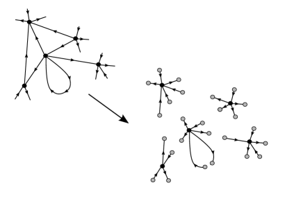
Figure 1: Splitting a directed graph $\Gamma$ into a disjoint union of vertex neighbourhoods.

Paths in a directed graph $\Gamma$ are morphisms in the free groupoid generated by $\Gamma$. They are described by words $w=e_{n}^{\epsilon_{n}}\circ\ldots\circ e_{1}^{\epsilon_{1}}$ with $n\in\mathbb{N}$, $e_{i}\in E$, $\epsilon_{i}\in\{\pm 1\}$ or empty words $\o_{v}$ for each vertex $v\in V$. A word $w$ is called composable if it is empty or if ${\bf t}(e_{i}^{\epsilon_{i}})={\bf s}(e_{i+1}^{\epsilon_{i+1}})$ for all $i=1,...,n-1$. In this case we set ${\bf s}(w)={\bf s}(e_{1}^{\epsilon_{1}})$ and ${\bf t}(w)={\bf t}(e_{n}^{\epsilon_{n}})$ and ${\bf s}(w)={\bf t}(w)=v$ if $w=\o_{v}$. The number $n\in\mathbb{N}$ is called the length of $w$. A word $w$ is called reduced if it is empty or of the form $w=e_{n}^{\epsilon_{n}}\circ\ldots\circ e_{1}^{\epsilon_{1}}$ with $e_{i}^{\epsilon_{i}}\neq e_{i+1}^{-\epsilon_{i+1}}$ for all $i\in\{1,...,n-1\}$.

Definition 2.15.

Let $\Gamma$ be a directed graph. The path groupoid $\mathcal{G}(\Gamma)$ is the free groupoid generated by $\Gamma$. Its objects are the vertices of $\Gamma$. A morphism from $u$ to $v$ is an equivalence class of composable words $w$ with ${\bf s}(w)=u$ and ${\bf t}(w)=v$ with respect to $e^{-1}\circ e\sim\o_{{\bf s}(e)}$, $e\circ e^{-1}\sim\o_{{\bf t}(e)}$ for all edges $e$ of $\Gamma$. Identity morphisms are equivalence classes of trivial words $\o_{v}$, and the composition of morphisms is induced by the concatenation. A path in $\Gamma$ is a morphism in $\mathcal{G}(\Gamma)$.

In the following, we consider directed graphs with additional structure, called ribbon graphs, fat graphs or embedded graphs (for background see [31, 21]). These are directed graphs with a cyclic ordering of the incident edge ends at each vertex, i. e. an ordering up to cyclic permutations.

This cyclic ordering equips the graph with the notion of a face. A path $p\in\mathcal{G}(\Gamma)$ given by a reduced word $e_{n}^{\epsilon_{n}}\circ\ldots\circ e_{1}^{\epsilon_{1}}$ is said to turn maximally right (left) at the vertex $v_{i}={\bf s}(e_{i+1}^{\epsilon_{i+1}})={\bf t}(e_{i}^{\epsilon_{i}})$ if the starting end of $e_{i+1}^{\epsilon_{i+1}}$ comes directly after (before) the target end of $e_{i}^{\epsilon_{i}}$ with respect to the cyclic ordering at $v_{i}$. If ${\bf s}(p)={\bf t}(p)=v_{n}$, $p$ is said to turn maximally right (left) at $v_{n}={\bf s}(e_{1}^{\epsilon_{1}})={\bf t}(e_{n}^{\epsilon_{n}})$ if the starting end of $e_{1}^{\epsilon_{1}}$ comes directly after (before) the target end of $e_{n}^{\epsilon_{n}}$ with respect to the cyclic ordering at $v_{n}$. Faces of $\Gamma$ are equivalence classes of closed paths that turn maximally right at each vertex and pass any edge at most once in each direction, up to cyclic permutations. The set of faces of $\Gamma$ is denoted $F(\Gamma)$

In the following, we also consider ribbon graphs in which some or all vertices are equipped with a linear ordering of the incident edge ends. In this case, we always require that the cyclic ordering induced by the linear ordering is the one from the ribbon graph structure. Any such linear ordering of the incident edge ends at a vertex is obtained from their cyclic ordering of the ribbon graph by selecting one of the incident edge ends as the edge end of minimal order. This is indicated in pictures by placing a marking, called cilium at the vertex and ordering the incident edges at the vertex counterclockwise from the cilium in the plane of the drawing, as shown in Figure 2. For a vertex $v$ with a linear odering of the incident edge ends, we write $e<f$ if $e,f$ are edge ends incident at $v$ and $e$ is of lower order than $f$.

Definition 2.16.

Let $\Gamma$ be a ribbon graph.

1. A ciliated vertex of $\Gamma$ is a vertex $v$ with a linear ordering of the incident edge ends that induces their cyclic ordering from the ribbon graph structure. Two edge ends $e,f$ at a ciliated vertex $v$ are called adjacent if there is no edge end $g$ at $v$ with $e<g<f$ or $f<g<e$. The valence $|v|$ of $v$ is the number of incident edge ends.
   

2. A ciliated ribbon graph is a ribbon graph in which all vertices are ciliated.
   

3. A ciliated face of $\Gamma$ is a closed path which turns maximally right at each vertex, including the starting vertex, and traverses each edge at most once in each direction. The valence $|f|$ of $f$ is its length as a reduced word in $E(\Gamma)$.
   

4. Two ciliated faces $f,f^{\prime}$ of $\Gamma$ are equivalent if they induce the same face, i. e. their expressions as reduced words in the edges of $\Gamma$ are related by cyclic permutations.

This terminology is compatible with Poincaré duality. By passing from a ribbon graph $\Gamma$ to its Poincaré dual $\bar{\Gamma}$, we can interpret a ciliated face of $\Gamma$ as a ciliated vertex of $\bar{\Gamma}$ and a ciliated vertex of $\Gamma$ as a ciliated face of $\bar{\Gamma}$. Vertices and faces of $\Gamma$ with the associated cyclic orderings are given as equivalence classes of ciliated vertices and faces under cyclic permutations and hence correspond to, respectively, faces and vertices of $\bar{\Gamma}$. In the following, we sometimes require that the ciliated ribbon graphs $\Gamma$ satisfy certain regularity conditions.

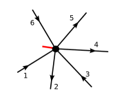
Figure 2: Vertex with incident edge ends and the ordering induced by the cilium.

Definition 2.17.

A ciliated ribbon graph $\Gamma$ is called regular if:

1. $\Gamma$ has no loops or multiple edges.

2. Each face of $\Gamma$ traverses each edge at most once.

3. Each face of $\Gamma$ contains exactly one cilium.

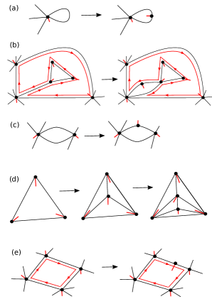
Figure 3: Regularising a ciliated ribbon graph: (a) Subdividing a loop, (b) doubling an edge, (c) subdividing multiple edges, (d) subdividing a face, (e) adding a ciliated vertex to a face.

Note that for a regular ciliated ribbon graph $\Gamma$, one has $|V(\Gamma)|=|F(\Gamma)|$. Each cilium corresponds to a pair $(v,f)$ of a ciliated vertex $v\in V(\Gamma)$ and a ciliated face $f$ based at the cilium. Such pairs $(v,f)$ are called sites in the context of Kitaev models.

The regularity conditions in Definition 2.17 are mild because any ciliated ribbon graph can be transformed into a regular ciliated ribbon graph by subdividing edges, doubling edges and subdividing faces. More precisely, for any ciliated ribbon graph $\Gamma$ one can construct a regular ciliated ribbon graph $\Gamma^{\prime}$ by the following procedure, illustrated in Figure 3:

1. Subdivide each loop by adding a bivalent ciliated vertex whose cilium points inside the loop, i. e. such that that the path along the loop that starts and ends at this new vertex and turns maximally right at each vertex becomes a ciliated face, as shown in Figure 3 (a).
   

2. Double each edge that is traversed twice by a face and add a ciliated bivalent vertex whose cilium points into the resulting face, as shown in Figure 3 (b).
   

3. For each pair of edges $e,e^{\prime}$ with ${\bf s}(e)={\bf s}(e^{\prime})$ and ${\bf t}(e)={\bf t}(e^{\prime})$, subdivide either $e$ or $e^{\prime}$ by adding a bivalent ciliated vertex, as shown in Figure 3 (c).
   

4. Subdivide each face that contains more than one cilium by adding a vertex and connecting it to the vertices of the face in such a way that each of the resulting faces contains at most one cilium. Equip the new vertex with a cilium and repeat if necessary, as shown in Figure 3 (d).
   

5. For each face that contains no cilia, add a bivalent ciliated vertex to one of its edges such that the cilium points into the face, as shown in Figure 3 (e).

Ribbon graphs can be viewed as graphs embedded into oriented surfaces. A graph embedded into an oriented surface inherits a cyclic ordering of the incident edge ends at each vertex from the orientation of the surface. Conversely, each ribbon graph defines oriented surface which is unique up to homeomorphisms and obtained as follows. Given a graph $\Gamma$, understood as a combinatorial graph, one obtains a graph in the topological sense, a 1-dimensional CW-complex, by gluing intervals to the vertices as specified by the edges. If additionally $\Gamma$ has a ribbon graph structure, one obtains an oriented surface $\Sigma_{\Gamma}$ by gluing a disc to each face of $\Gamma$. If $\Gamma$ is a graph embedded in an oriented surface $\Sigma$ and equipped with the induced ribbon graph structure, then the surface $\Sigma_{\Gamma}$ is homeomorphic to $\Sigma$ if and only if each connected component of $\Sigma\setminus\Gamma$ is homeomorphic to a disc.

Ribbon graphs $\Gamma$ and $\Gamma^{\prime}$ that are related by certain graph operations define homeomorphic surfaces $\Sigma_{\Gamma}$ and $\Sigma_{\Gamma^{\prime}}$. These graph operations include edge contractions, edge subdivisions, subdivisions of faces, doubling edges and adding or removing edges from the graph if this does not change the number of connected components [31, 21, 38]. This implies in particular that for each ciliated ribbon graph $\Gamma$ there is a ciliated ribbon graph $\Gamma^{\prime}$ that is regular in the sense of Definition 2.17 and such that $\Sigma_{\Gamma}$ and $\Sigma_{\Gamma^{\prime}}$ are homeomorphic.

3 Kitaev models

Kitaev models were first introduced in [28]. They were then generalised to models based on the group algebra of a finite group and with defects and domain walls in [13] and to finite-dimensional semisimple Hopf algebras in [15]. More recent generalisations include models based on certain certain tensor categories and with defect data from higher categories [29]. In this article we focus on the models from [15] for a finite-dimensional semisimple Hopf algebra $H$.

The two ingredients of a Kitaev model are a finite-dimensional semisimple Hopf algebra $H$ and a ribbon graph $\Gamma$. The starting point in the construction is the extended space $H^{\otimes E}$ obtained by associating a copy of $H$ to each edge of $\Gamma$. One then assigns to each edge $e\in E$ four basic triangle operators $L^{h}_{e\pm}:H\to H$ and $T^{\alpha}_{e\pm}:H\to H$, indexed by elements $h\in H$ and $\alpha\in H^{*}$. With the notation and conventions from Section 2.1 they are defined as follows.

Definition 3.1 ([28, 15]).

Let $H$ be a finite-dimensional semisimple Hopf algebra and $\Gamma$ a ribbon graph. The triangle operators for an edge $e$ of $\Gamma$, $h\in H$ and $\alpha\in H^{*}$ are the linear maps

$$L^{h}_{e\pm}=(L^{h}_{\pm})_{e}:H^{\otimes E}\to H^{\otimes E}\qquad\qquad T^{\alpha}_{e\pm}=(T^{\alpha}_{\pm})_{e}:H^{\otimes E}\to H^{\otimes E},$$

with $L^{h}_{\pm},T^{\alpha}_{\pm}:H\to H$ given by

$$L_{+}^{h}k=h\cdot k L_{-}^{h}k=(S\circ L_{+}^{S(h)}\circ S)k=k\cdot h$$ (12)

$$T^{\alpha}_{+}k=\langle\alpha,{k}_{({2})}\rangle\,{k}_{({1})} T^{\alpha}_{-}k=(S\circ T^{S(\alpha)}_{+}\circ S)k=\langle\alpha,{k}_{({1})}\rangle\,{k}_{({2})}.$$

By combining the triangle operators of the edges at each vertex $v$ and in each face $f$ of $\Gamma$, one obtains the vertex and face operators $A_{v}^{h}:H^{\otimes E}\to H^{\otimes E}$ and $B^{\alpha}_{f}:H^{\otimes E}\to H^{\otimes E}$. Their definition requires a linear ordering of the incident edges at each vertex and a in each face, i. e. ciliated vertices and ciliated faces. They are defined for general ribbon graphs $\Gamma$, but in the following we restrict attention to ribbon graphs without loops or multiple edges.

Definition 3.2 ([28, 15] ).

Let $\Gamma$ be a ribbon graph without loops or multiple edges.

1. Let $v$ be a ciliated vertex of $\Gamma$ with incident edges $e_{1},...,e_{n}$, numbered according to the ordering at $v$ and such that $e_{1}^{\epsilon_{1}}$,…, $e_{n}^{\epsilon_{n}}$ are incoming. The vertex operator $A^{h}_{v}:H^{\otimes E}\to H^{\otimes E}$ for $h\in H$ is the linear map

   $$A^{h}_{v}=L^{S^{\tau_{1}}({h}_{({1})})}_{e_{1}\epsilon_{1}}\circ\ldots\circ L^{S^{\tau_{n}}({h}_{({n})})}_{e_{n}\epsilon_{n}}:H^{\otimes E}\to H^{\otimes E}\qquad\text{with}\;\;\;\tau_{i}=\tfrac{1}{2}(1-\epsilon_{i}).$$

2. Let $f=e_{1}^{\epsilon_{1}}\circ\ldots\circ e_{n}^{\epsilon_{n}}$ be a ciliated face of $\Gamma$. The face operator $B^{\alpha}_{f}:H^{\otimes E}\to H^{\otimes E}$ for $\alpha\in H^{*}$ is the linear map

   $$B^{\alpha}_{f}=T^{S^{\tau_{1}}({\alpha}_{({1})})}_{e_{1}\epsilon_{1}}\circ\ldots\circ T^{S^{\tau_{n}}({\alpha}_{({n})})}_{e_{n}\epsilon_{n}}:H^{\otimes E}\to H^{\otimes E}\qquad\text{with}\;\;\;\tau_{i}=\tfrac{1}{2}(1-\epsilon_{i}).$$

Choosing a cilium at a vertex $v$ does not only equip $v$ with the structure of a ciliated vertex but at the same time selects a ciliated face of $\Gamma$, namely the unique ciliated face that starts and ends at the cilium at $v$. It was shown in [15] that the associated vertex and face operators define a representation of the Drinfeld double $D(H)$. This follows by a direct computation from the definition of the vertex and face operators and equation (12) for the triangle operators and is proven in Section 5.3 in a different formalism.

Lemma 3.3 ([28, 15]).

Let $v$ be a ciliated vertex of $\Gamma$ and $f(v)$ the ciliated face of $\Gamma$ that starts and ends at the cilium at $v$. The associated vertex and face operators satisfy the commutation relations

$$A^{h}_{v}\circ A^{k}_{v}=A_{v}^{hk}\qquad B^{\alpha}_{f(v)}\circ B^{\beta}_{f(v)}=B^{\alpha\beta}_{f(v)}\qquad A^{h}_{v}\circ B^{\alpha}_{f(v)}=\langle{\alpha}_{({3})},{h}_{({1})}\rangle\langle{\alpha}_{({1})},S({h}_{({3})})\rangle\;B^{{\alpha}_{({2})}}_{f(v)}\circ A^{{h}_{({2})}}_{v}.$$

The map $\tau:D(H)\to\mathrm{End}_{\mathbb{F}}(H)$, $\alpha\otimes h\mapsto B^{\alpha}_{f(v)}\circ A^{h}_{v}$ is an injective algebra homomorphism.

Similarly one can show that for any choice of the cilia the vertex operators for different vertices $v,w$ and the faces operators for different faces $f,g$ of $\Gamma$ commute and that the vertex operators commute with all face operators that satisfy a certain condition on the cilia.

Lemma 3.4 ([28, 15]).

Let $\Gamma$ be a ciliated ribbon graph, $h,k\in H$ and $\alpha,\beta\in H^{*}$.

1. For all choices of the ciliation, one has $A_{v}^{h}\circ A_{w}^{k}=A^{k}_{w}\circ A^{h}_{v}$ if $v\neq w$.

2. For all choices of the ciliation, one has $B_{f}^{\alpha}\circ B_{g}^{\beta}=B_{g}^{\beta}\circ B^{\alpha}_{f}$ if $f\neq g$.

3. If $v$ is a ciliated vertex and $f$ a ciliated face that is not based at $v$ and does not traverse the cilium at $v$, then $A^{h}_{v}\circ B^{\alpha}_{f}=B^{\alpha}_{f}\circ A^{h}_{v}$.

If one chooses for $h\in H$ the Haar integral $\ell\in H$ and for $\alpha\in H^{*}$ the Haar integral $\eta\in H^{*}$, the associated vertex and face operators $A^{\ell}_{v},B^{\eta}_{f}:H^{\otimes E}\to H^{\otimes E}$ no longer depend on the choice of the cilia at $v$ and at $f$. This is a direct consequence of the properties of the Haar integral in Remark 2.4. The properties of the Haar integral also imply that they are projectors with images

$$A^{\ell}_{v}(H^{\otimes E})=\{x\in H^{\otimes E}:\,A^{h}_{v}x=\epsilon(h)x\;\forall h\in H\}\quad B^{\eta}_{f}(H^{\otimes E})=\{x\in H^{\otimes E}:\,B^{\alpha}_{f}x=\epsilon(\alpha)x\;\forall\alpha\in H^{*}\}$$

and that their commutation relations from Lemma 3.3 simplify to the following.

Lemma 3.5 ([28, 15]).

Denote by $\ell\in H$, $\eta\in H^{*}$ the Haar integrals of $H$ and $H^{*}$. Then the vertex and face operators $A^{\ell}_{v}$, $B^{\eta}_{f}$ do not depend on the cilia and form a set of commuting projectors.

Definition 3.6 ([28, 15]).

Let $\Gamma$ be a ribbon graph, $H$ a finite-dimensional semisimple Hopf algebra and $\ell\in H$, $\eta\in H^{*}$ the Haar integrals of $H$ and $H^{*}$. The Hamiltonian of the Kitaev model on $\Gamma$ is

$$H_{\mathrm{K}}=\Pi_{v\in V}A^{\ell}_{v}\circ\Pi_{f\in F}B^{\eta}_{f}:H^{\otimes E}\to H^{\otimes E}.$$

Its image is the protected space

$$\mathcal{H}_{\mathrm{pr}} =H_{\mathrm{K}}(H^{\otimes E})=\{h\in H^{\otimes E}:H_{\mathrm{K}}(h)=h\}.$$

It was shown in [28, 15] that the protected space is a topological invariant. It depends only on the homeomorphism class of the oriented surface $\Sigma_{\Gamma}$ obtained by gluing discs to the faces of $\Gamma$. Topological excitations in Kitaev models are obtained by removing the vertex and face operators $A^{\ell}_{v}$ and $B^{\ell}_{f}$ from the Hamiltonian $H_{\mathrm{K}}$ for a fixed number of sites $(v,f)$ which have no vertices or faces in common. This yields another projector $H_{\mathrm{K}}^{\prime}$ whose ground state $H_{\mathrm{K}}^{\prime}(H^{\otimes E})=\{h\in H^{\otimes E}:H_{\mathrm{K}}^{\prime}(h)=h\}$ describes a model with excitations labelled by representations of the Drinfeld double $D(H)$.

While Kitaev models are mostly formulated in terms of operators acting on Hilbert spaces, we take a more algebraic viewpoint and focus on algebra structures and not on specific representations. For this we note that the triangle operators $L^{y}_{e\pm},T^{\alpha}_{e\pm}:H^{\otimes E}\to H^{\otimes E}$ for an edge $e$ of $\Gamma$ form a faithful representation of the Heisenberg double $\mathcal{H}(H)$ from Definition 2.11. This allows one to identify Kitaev’s edge operator algebra with the $E$-fold tensor product $\mathcal{H}(H)^{\otimes E}$.

Lemma 3.7.

Let $H$ be a finite-dimensional semisimple Hopf algebra with dual $H^{*}$. Denote by $S$ the antipodes of $H$ and $H^{*}$ and by $S_{D}:H\otimes H^{*}\to H\otimes H^{*}$ the antipode of $D(H)^{*}$ from (2).

1. The linear isomorphism $\phi:\mathcal{H}(H)\to\mathrm{End}_{\mathbb{F}}(H)$, $\phi(y\otimes\alpha)h=(L^{y}_{+}\circ T^{\alpha}_{+})h=\langle\alpha,{h}_{({2})}\rangle\,y\cdot{h}_{({1})}$ defines a cyclic $\mathcal{H}(H)$-left module structure on $H$.
   

2. The triangle operators $L^{y}_{\pm},T^{\alpha}_{\pm}:H\to H$ from (12) are given by

   $$L^{y}_{+}=\phi(y\otimes 1) T^{\alpha}_{+}=\phi(1\otimes\alpha) L^{y}_{-}=\phi\circ S_{D}(S(y)\otimes 1) T^{\alpha}_{-}=\phi\circ S_{D}(1\otimes S(\alpha)).$$

3. The linear map $\rho=\phi^{\otimes E}:\mathcal{H}(H)^{\otimes E}\to\mathrm{End}_{\mathbb{F}}(H^{\otimes E})\cong\mathrm{End}_{\mathbb{F}}(H)^{\otimes E}$ is an algebra isomorphism.

Proof.

That $\phi$ defines an $\mathcal{H}(H)$-left module structure on $H$ follows by a direct computation from the properties of the left and right regular action of $H$ on itself and on $H^{*}$ in Definition 2.5 and the multiplication of the Heisenberg double in (6). That the module is cyclic follows from the identity $h=\phi(h\otimes 1)1$ for all $h\in H$. To show that $\phi$ is an isomorphism, it is sufficient to show that it is surjective. This can be seen as follows. Let $\{x_{i}\}$ be a basis of $H$ and $\{\alpha^{i}\}$ the dual basis of $H^{*}$ and $\ell\in H$, $\eta\in H^{*}$ the Haar integrals. The properties of the Haar integral from Remark 2.4 imply

$$\phi((x_{i}\otimes\eta)\cdot(\ell\otimes\alpha^{j}))x_{k}=\langle{\eta}_{({1})},{\ell}_{({2})}\rangle\,\phi(x_{i}{\ell}_{({1})}\otimes{\eta}_{({2})}\alpha^{j})x_{k}=\langle{\eta}_{({1})},{\ell}_{({2})}\rangle\langle{\eta}_{({2})}\alpha^{j},x_{k(2)}\rangle\,x_{i}{\ell}_{({1})}x_{k(1)}$$

$$=\langle\eta,{\ell}_{({2})}x_{k(2)}\rangle\langle\alpha^{j},x_{k(3)}\rangle x_{i}{\ell}_{({1})}x_{k(1)}=\langle\eta,\ell x_{k(1)}\rangle\langle\alpha^{j},x_{k(2)}\rangle\,x_{i}=\epsilon(x_{k(1)})\,\langle\eta,\ell\rangle\,\langle\alpha^{j},x_{k(2)}\rangle x_{i}=\langle\eta,\ell\rangle\,\delta^{j}_{k}x_{i}.$$

As the Haar integrals satisfy $\langle\eta,\ell\rangle\neq 0$ and the linear maps $\phi_{ij}\in\mathrm{End}_{\mathbb{F}}(H)$ with $\phi_{ij}(x_{k})=\delta^{j}_{k}x_{i}$ form a basis of $\mathrm{End}_{\mathbb{F}}(H)$, this proves that $\phi$ is surjective. The formulas in (12) for $L^{y}_{+}$ and $T^{\alpha}_{+}$ are obtained directly from the definition of $\phi$. The ones for $L^{y}_{\pm}$ and $T^{\alpha}_{\pm}$ follow from the definition of the antipode of $D(H)^{*}$ in (2), which yields

$$\phi\circ S_{D}\circ(S\otimes\mathrm{id})(y\otimes 1)=\Sigma_{i,j}\phi(x_{i}yS(x_{j})\otimes\alpha^{j}\alpha^{i})=\Sigma_{i,j}\;L_{+}^{x_{i}yS(x_{j})}\circ T^{\alpha^{j}\alpha^{i}}_{+}$$

$$\phi\circ S_{D}\circ(\mathrm{id}\otimes S)(1\otimes\alpha)=\Sigma_{i,j}\phi(x_{i}S(x_{j})\otimes\alpha^{j}\alpha\alpha^{i})=\Sigma_{i,j}\;L_{+}^{x_{i}S(x_{j})}\circ T^{\alpha^{j}\alpha\alpha^{i}}_{+}.$$

This implies for all $h\in H$

$$\phi\circ S_{D}(S(y)\otimes 1)h=\Sigma_{i,j}\,\langle\alpha^{j}\alpha^{i},{h}_{({2})}\rangle x_{i}yS(x_{j}){h}_{({1})}={h}_{({3})}yS({h}_{({2})}){h}_{({1})}=h\cdot y=L^{y}_{-}h$$

$$\phi\circ S_{D}(1\otimes S(\alpha))h=\Sigma_{i,j}\,\langle\alpha^{j}\alpha\alpha^{i},{h}_{({2})}\rangle x_{i}S(x_{j}){h}_{({1})}=\langle\alpha,{h}_{({3})}\rangle\,{h}_{({4})}S({h}_{({2})}){h}_{({1})}=\langle\alpha,{h}_{({1})}\rangle\,{h}_{({2})}=T^{\alpha}_{-}h.$$

The last claim follows from the fact that $L^{y}_{e\pm}$, $T^{\alpha}_{e\pm}$ commute with $L^{y}_{f\pm}$, $T^{\alpha}_{f\pm}$ if $e\neq f$. ∎

4 Hopf algebra gauge theory

The action of vertex and face operators in the Kitaev models on the extended space resemble gauge symmetries. They define representations of the Hopf algebras $H$, $H^{*}$ and $D(H)$ on the extended space $H^{\otimes E}$, and the protected space $\mathcal{H}_{\mathrm{pr}}$ is defined as the set of states that transform trivially under these representations. This suggests that Kitaev models could be understood as a Hopf algebra analogue of a lattice gauge theory.

This requires a concept of a Hopf algebra valued gauge theory on a ribbon graph. An axiomatic description of such a Hopf algebra gauge theory was derived in [38] by generalising lattice gauge theory for a finite group. It is shown there that the resulting Hopf algebra gauge theory coincides with the algebras obtained in [1, 2, 3] and [17, 18] via the combinatorial quantisation of Chern-Simons gauge theory, which were analysed further in [19]. We summarise the description in [38] but with a change of notation and for ribbon graphs without loops or multiple edges.

The general definition of a Hopf algebra gauge theory is obtained by linearising the corresponding structures for a gauge theory based on a finite group. A lattice gauge theory for a ribbon graph $\Gamma$ and a finite group $G$ consists of the following:

• gauge fields and functions of gauge fields: A gauge field is an assignment of an element $g_{e}\in G$ to each oriented edge $e\in E$ and hence can be interpreted as an element of the set $G^{\times E}$. Functions of the gauge fields with values in $\mathbb{F}$ form a commutative algebra $\mathrm{Fun}(G^{\times E})$ with respect to pointwise multiplication and addition. They are related to gauge fields by an evaluation map $\mathrm{ev}:\mathrm{Fun}(G^{\times E})\times G^{\times E}\to\mathbb{F}$, $(f,g)\mapsto f(g)$.
  

• gauge transformations: A gauge transformation is an assignment of a group element $g_{v}$ to each vertex $v\in V$. Gauge transformations at different vertices commute and the composition of gauge transformations at a given vertex is given by the group multiplication in $G$. A gauge transformation can therefore be viewed as an element of the group $G^{\times V}$.
  

• action of gauge transformations: Gauge transformations act on gauge fields via a left action $\rhd:G^{\times V}\times G^{\times E}\to G^{\times E}$. This action is local: a gauge transformation at a vertex $v$ acts only on the components of gauge fields associated with edges at $v$. This action is given by left multiplication and right multiplication for outgoing and incoming edges. The left action of gauge transformations on gauge fields induces a right action $\lhd:\mathrm{Fun}(G^{\times E})\times G^{\times V}\to\mathrm{Fun}(G^{\times E})$ defined by $(f\lhd h)(g)=f(h\rhd g)$ for all $f\in\mathrm{Fun}(G^{\times E})$, $g\in G^{\times E}$ and $h\in G^{\times V}$.
  

• observables: The physical observables are the gauge invariant functions $f\in\mathrm{Fun}(G^{\times E})$ with $f\rhd h=f$ for all $h\in G^{\times V}$. They form a subalgebra of the commutative algebra $\mathrm{Fun}(G^{\times E})$.

The corresponding structures for lattice gauge theories with values in a finite-dimensional Hopf algebra $K$ were obtained in [38] by linearising the structures for a finite group $G$.

• gauge fields and functions of gauge fields: The set $G^{\times E}$ of gauge fields is replaced by the vector space $K^{\otimes E}$. Functions of gauge fields are identified with elements of the dual vector space $K^{*\otimes E}$, and the evaluation map is replaced by the pairing $\langle\,,\,\rangle:K^{*\otimes E}\otimes K^{\otimes E}\to\mathbb{F}$. One also requires an algebra structure on $K^{*\otimes E}$, although not necessarily the canonical one.
  

• gauge transformations: The group $G^{\times V}$ of gauge transformations is replaced by the Hopf algebra $K^{\otimes V}$ of gauge transformations.
  

• action of gauge transformations: The action of gauge transformations on gauge fields takes the form of a $K^{\otimes V}$-left module structure $\rhd:K^{\otimes V}\otimes K^{\otimes E}\to K^{\otimes E}$. This action must be local in the sense that the component of a gauge transformation associated with a vertex $v$ acts only on the components of gauge fields associated with edges incident at $v$. Instead of the action of $G$ on itself by left and right multiplication, it is given by the left and right regular action of $K$ on itself for incoming and outgoing edges at $v$. Via the pairing, this $K^{\otimes V}$-left module structure induces a $K^{\otimes V}$-right module structure on the vector space $K^{*\otimes E}$, which is given by the left and right regular action of $K$ on $K^{*}$ for incoming and outgoing edges at $v$.
  

• observables: The gauge invariant functions or observables of the Hopf algebra gauge theory are defined as the invariants of the $K^{\otimes V}$-right module structure on $K^{*\otimes E}$, the elements $\alpha\in K^{*\otimes E}$ with $\alpha\lhd h=\epsilon(h)\,\alpha$ for all $h\in K^{\otimes V}$. They must form a subalgebra of $K^{*\otimes E}$.

The fundamental difference between a Hopf algebra gauge theory and a group gauge theory is that generally one cannot equip the vector space $K^{*\otimes E}$ with the canonical algebra structure induced by the tensor product. To ensure that the invariants of the $K^{\otimes V}$-right module $K^{*\otimes E}$ form not only a linear subspace but a subalgebra of $K^{*\otimes E}$, the algebra structure on $K^{*\otimes E}$ must chosen in such a way that $K^{*\otimes E}$ is not only a $K^{\otimes V}$-right module but a $K^{\otimes V}$-right module algebra over $K^{\otimes E}$. This is not the case for the canonical algebra structure on $K^{*\otimes E}$ unless $K$ is cocommutative.

This shows that the essential mathematical structure in a Hopf algebra gauge theory is a $K^{\otimes V}$-right module algebra structure on the vector space $K^{*\otimes E}$. It was shown in [38] that such a $K^{\otimes V}$-right module algebra structure, subject to certain additional locality conditions, can be built up from local Hopf algebra gauge theories on the vertex neighbourhoods of $\Gamma$.

By definition, a Hopf algebra gauge theory on the vertex neighbourhood $\Gamma_{v}$ of an $n$-valent vertex $v$ is a $K$-right module algebra structure on $K^{*\otimes n}$. It is shown in [38] that the natural algebraic ingredient for a Hopf algebra gauge theory on $\Gamma_{v}$ is a ribbon Hopf algebra $K$. A quasitriangular structure on $K$ is required for the $K$-module algebra structure on $K^{*\otimes n}$ is all edges are incoming.

The condition that $K$ is ribbon is needed for the reversal of edge orientation. As we consider only the case of a finite-dimensional semisimple Hopf algebra $K$ over a field of characteristic zero, quasi-triangularity of $K$ implies that $K$ is ribbon [22] and edge orientation is reversed with the antipode $S:K^{*}\to K^{*}$. The $K$-right module algebra structure on $K^{*\otimes n}$ is then defined by the following theorem, which makes use of the ‘braided tensor product’ introduced in [11, 35].

Theorem 4.1 ([38]).

Let $K$ be a finite-dimensional semisimple quasitriangular Hopf algebra with $R$-matrix $R\in K\otimes K$ and $\sigma_{i}\in\{0,1\}$ for $i\in\{1,...,n\}$. Then the multiplication law

$$(\alpha)_{i}\cdot(\beta)_{i}=\begin{cases}\langle\beta_{(1)}\otimes\alpha_{(1)},R\rangle\,({\beta}_{({2})}{\alpha}_{({2})})_{i}&\sigma_{i}=0\\ (\alpha\beta)_{i}&\sigma_{i}=1\end{cases}$$ (13)

$$(\alpha)_{i}\cdot(\beta)_{j}=\begin{cases}\langle\beta_{(1)}\otimes\alpha_{(1)},R\rangle\,(\alpha_{(2)}\otimes\beta_{(2)})_{ij}&i>j\\ (\alpha\otimes\beta)_{ij}&i<j,\end{cases}$$

and the linear map $\lhd:K^{*\otimes n}\otimes K\to K^{*\otimes n}$

$$(\alpha^{1}\otimes...\otimes\alpha^{n})\lhd h=\langle\alpha^{1}_{(1)}\cdots\alpha^{n}_{(1)},h\rangle\;\alpha^{1}_{(2)}\otimes\ldots\otimes\alpha^{n}_{(2)}$$ (14)

define a $K$-right module algebra structure on $K^{*\otimes n}$.

A Hopf algebra gauge theory for a vertex neighbourhood of a ciliated vertex $v$ with $n$ incident edge ends is then obtained as follows. The edge ends at $v$ are numbered according to the ordering at $v$ as in Figure 2, and the $i$th copy of $K^{*}$ in $K^{*\otimes n}$ is associated with the $i$th edge end at $v$. One chooses arbitrary parameters $\sigma_{i}\in\{0,1\}$ and sets $\tau_{i}=0$ if the $i$th edge end is incoming at $v$ and $\tau_{i}=1$ if it is outgoing for $i\in\{1,...,n\}$. The $K$-right module algebra structure from Theorem 4.1 is then modified with the involution $S^{\tau_{1}}\otimes...\otimes S^{\tau_{n}}:K^{*\otimes n}\to K^{*\otimes n}$ to take into account edge orientation.

Definition 4.2 ([38]).

Let $v$ be a ciliated vertex with $n$ incident edge ends. The $K$-right module algebra structure $\mathcal{A}^{*}_{v}$ of a Hopf algebra gauge theory on $\Gamma_{v}$ is defined by the condition that the involution $S^{\tau_{1}}\otimes\ldots\otimes S^{\tau_{n}}:K^{*\otimes n}\to\mathcal{A}^{*}_{v}$ is a morphism of $K$-right module algebras when $K^{*\otimes n}$ is equipped with the $K$-right module algebra structure in Theorem 4.1.

The parameters $\sigma_{i}\in\{0,1\}$ can be chosen arbitrarily at this stage but play an essential role in gluing together the Hopf algebra gauge theories on different vertex neighbourhoods to a Hopf algebra gauge theory on $\Gamma$. This is achieved by embedding the vector space $K^{*\otimes E}$ into the tensor product $\otimes_{v\in V}A^{*}_{v}$ via the injective linear map

$$G^{*}=\otimes_{e\in E}G^{*}_{e}:\,K^{*\otimes E}\to\otimes_{v\in V}K^{*\otimes|v|},\quad(\alpha)_{e}\mapsto({\alpha}_{({2})}\otimes{\alpha}_{({1})})_{s(e)t(e)}.$$ (15)

Note that this map is dual to the map $G:K^{\otimes 2E}\to K^{\otimes E}$, $(\alpha\otimes\beta)_{t(e)s(e)}\to(\alpha\cdot\beta)_{e}$ that assigns to an edge $e\in E(\Gamma)$ the product of the components of a gauge field of the edge ends $s(e)\in E(\Gamma_{{\bf s}(e)})$ and $t(e)\in E(\Gamma_{{\bf t}(e)})$. As the vertex neighbourhoods are obtained by splitting the edge $e\in E(\Gamma)$ into the edge ends $s(e)$ and $t(e)$, this is natural and intuitive from the perspective of gauge theory.

To define a local Hopf algebra gauge theory on $\Gamma$, one then assigns a universal $R$-matrix $R_{v}$ to each vertex $v$ and selects for each edge $e\in E(\Gamma)$ one of the associated edge ends $t(e),s(e)\in\cup_{v\in V}E(\Gamma_{v})$. This determines a map ${\boldsymbol{\rho}}:E(\Gamma)\to\cup_{v\in V}E(\Gamma_{v})$, and for each edge end $f\in\cup_{v\in V}E(\Gamma_{v})$ one sets $\sigma_{f}=0$ if $f$ is in the image of ${\boldsymbol{\rho}}$ and $\sigma_{f}=1$ else. This defines a Hopf algebra gauge theory on each vertex neighbourhood $\Gamma_{v}$ and a $K^{\otimes V}$-right module algebra $\otimes_{v\in V}\mathcal{A}^{*}_{v}$. The $K^{\otimes V}$-module algebra structure of the vector space $K^{*\otimes E}$ is then obtained from the following theorem.

Theorem 4.3 ([38]).

Let $K$ be a finite-dimensional semisimple quasitriangular Hopf algebra and $\Gamma$ a ciliated ribbon graph without loops or multiple edges and equipped with the data above. Then:

1. $G^{*}(K^{*\otimes E})\subset\otimes_{v\in V}\mathcal{A}^{*}_{v}$ is a subalgebra and a $K^{\otimes V}$-submodule of $\otimes_{v\in V}\mathcal{A}^{*}_{v}$.
   

2. The induced $K^{\otimes V}$-right module algebra structure on $K^{*\otimes E}$ is a Hopf algebra gauge theory on $\Gamma$.
   

3. If $R_{v}=R$ for all $v\in V$, the $K^{\otimes V}$-right module algebra structure on $K^{*\otimes E}$ does not depend on the choice of ${\boldsymbol{\rho}}$.
   

The vector space $K^{*\otimes E}$ with this $K^{\otimes V}$-module algebra structure is denoted $\mathcal{A}^{*}_{\Gamma}$, and its elements are called functions. Elements of the vector space $K^{\otimes E}$ are called gauge fields, and elements of the Hopf algebra $K^{\otimes V}$ gauge transformations. The invariants of $\mathcal{A}^{*}_{\Gamma}$ are called gauge invariant functions or observables.

In the following, we restrict attention to local Hopf algebra gauge theories in which the same $R$-matrix is assigned to each vertex $v$ and to loop-free ribbon graphs $\Gamma$ without multiple edges. An explicit description of the algebra $\mathcal{A}^{*}_{\Gamma}$ in terms of generators and multiplication relations is given in [38, Lemma 3.20]. For the case at hand, we can summarise the relations from [38, Lemma 3.20] and the $K^{\otimes V}$-module structure on $\mathcal{A}^{*}_{\Gamma}$ in the notation from Section 2.1 as follows.

Proposition 4.4 ([38]).

Let $K$ be a finite-dimensional semisimple quasitriangular Hopf algebra and $\Gamma$ a ciliated ribbon graph without loops or multiple edges. Assign the same $R$-matrix $R\in K\otimes K$ to each vertex $v\in V(\Gamma)$. Then the algebra $\mathcal{A}^{*}_{\Gamma}$ is generated by the elements $(\alpha)_{e}$ for the edges $e$ of $\Gamma$ and $\alpha\in K^{*}$, subject to the following relations:

• $(\beta)_{e}\cdot(\alpha)_{e}=\langle{\alpha}_{({1})}\otimes{\beta}_{({1})},R\rangle\,({\alpha}_{({2})}{\beta}_{({2})})_{e}$ for all edges $e$ of $\Gamma$,
  

• $(\beta)_{f}\cdot(\alpha)_{e}=(\alpha)_{e}\cdot(\beta)_{f}$ if the edges $e,f$ have no vertex in common,
  

• $(\beta)_{f}\cdot(\alpha)_{e}=\langle S^{\tau_{e}}({\alpha}_{({1+\tau_{e}})})\otimes S^{\tau_{f}}({\beta}_{({1+\tau_{f}})},R\rangle\,({\beta}_{({2-\tau_{f}})})_{f}\cdot({\alpha}_{({2-\tau_{e}})})_{e}$ for edges $e,f$ with a common vertex $v$, where $\tau_{h}=0$ if $h$ is incoming at $v$ and $\tau_{h}=1$ if $h$ is outgoing.

Its $K^{\otimes V}$-module structure is given by $(\alpha)_{e}\lhd(h)_{v}=\epsilon(h)(\alpha)_{e}$ for $v\notin\{{\bf s}(e),{\bf t}(e)\}$, $(\alpha)_{e}\lhd(h)_{{\bf t}(e)}=\langle{\alpha}_{({1})},h\rangle(\alpha)_{e}$ and $(\alpha)_{e}\lhd(h)_{{\bf s}(e)}=\langle S({\alpha}_{({2})}),h\rangle(\alpha)_{e}$ for all $\alpha\in K^{*\otimes E}$ and $h\in K^{\otimes V}$.

By Lemma 2.10 the gauge invariant functions, which are the invariants of the $K^{\otimes V}$-right module algebra $K^{*\otimes E}$, form a subalgebra $\mathcal{A}^{*}_{\Gamma\,inv}\subset\mathcal{A}^{*}_{\Gamma}$. It is shown in [38] that this subalgebra is independent of the choice of the cilia and depends only on the homeomorphism class of the surface $\dot{\Sigma}_{\Gamma}$ obtained by gluing annuli to the faces of $\Gamma$.

Theorem 4.5 ([38]).

Let $K$ be a finite-dimensional semisimple quasitriangular Hopf algebra with Haar integral $\ell$ and $\Gamma$ a ciliated ribbon graph. Then $\mathcal{A}^{*}_{\Gamma\,inv}$ is a subalgebra of $\mathcal{A}^{*}_{\Gamma}$ and depends only on the homeomorphism class of $\dot{\Sigma}_{\Gamma}$. The map $P_{inv}:\mathcal{A}^{*}_{\Gamma}\to\mathcal{A}^{*}_{\Gamma}$, $\alpha\mapsto\alpha\lhd\ell^{\otimes V}$ is a projector on $\mathcal{A}^{*}_{\Gamma\,inv}$.

Besides gauge invariance, there is another essential concept in a lattice gauge theory, namely curvature. In a classical gauge theory on an oriented surface curvature is locally a 2-form and hence can be integrated over discs on the surface. In a description based on a ribbon graph $\Gamma$, these discs correspond to the faces of $\Gamma$. Hence, curvature in a Hopf algebra gauge theory is described by Hopf algebra valued holonomies of faces of $\Gamma$.

On the level of gauge fields, holonomy is an assignment of a linear map $\mathrm{Hol}_{p}:K^{\otimes E}\to K$ to each path $p\in\mathcal{G}(\Gamma)$. In the dual picture for functions this corresponds to an assignment of a linear map $\mathrm{Hol}_{p}:K^{*}\to K^{*\otimes E}$ to each path $p\in\mathcal{G}(\Gamma)$. This assignment must be compatible with trivial paths, composition of paths and inverses and hence define a functor $\mathrm{Hol}:\mathcal{G}(\Gamma)\to\mathrm{Hom}_{\mathbb{F}}(K^{*},K^{*\otimes E})$, where $\mathrm{Hom}_{\mathbb{F}}(K^{*},K^{*\otimes E})$ is equipped with the structure of an $\mathbb{F}$-linear category with a single object, i. e. with an associative algebra structure over $\mathbb{F}$. This was defined in [38] as a convolution product. For any algebra $(A,m,1)$ and coalgebra $(C,\Delta,\epsilon)$ over $\mathbb{F}$ the convolution product

$$\bullet:\mathrm{Hom}_{\mathbb{F}}(C,A)\otimes\mathrm{Hom}_{\mathbb{F}}(C,A)\to\mathrm{Hom}_{\mathbb{F}}(C,A),\quad\phi\otimes\psi\mapsto\phi\bullet\psi=m\circ(\phi\otimes\psi)\circ\Delta,$$ (16)

defines an associative algebra structure on $\mathrm{Hom}_{\mathbb{F}}(C,A)$ with unit $\epsilon\,1$. It is argued in [38] that the natural choice of $A$ and $C$ for a Hopf algebra gauge theory are $A=K^{*\otimes E}$ and $C=K^{*}$, with the canonical algebra and coalgebra structure. As the path groupoid $\mathcal{G}(\Gamma)$ is generated by the edges of $\Gamma$, a functor $\mathrm{Hol}:\mathcal{G}(\Gamma)\to\mathrm{Hom}_{\mathbb{F}}(K^{*},K^{*\otimes E})$ is defined uniquely by its values on the paths $e^{\pm 1}\in\mathcal{G}(\Gamma)$ for $e\in E$. For these paths it is natural to choose $\mathrm{Hol}_{e}=\iota_{e}$ and $\mathrm{Hol}_{e^{-1}}=\iota_{e}\circ S$, where $\iota_{e}:K^{*}\to K^{*\otimes E}$, $\alpha\mapsto(\alpha)_{e}$ is the map that sends an element $\alpha\in K^{*}$ to the pure tensor $(\alpha)_{e}\in K^{*\otimes E}$ that has the entry $\alpha$ in the component of $K^{*}$ associated with $e\in E$ and $1$ in all other components, as defined at the beginning of Section 2.1.

Definition 4.6 ([38]).

Let $\Gamma$ be a ciliated ribbon graph and $K$ a finite-dimensional semisimple quasitriangular Hopf algebra. Equip $\mathrm{Hom}_{\mathbb{F}}(K^{*},K^{*\otimes E})$ with the algebra structure (16) for $A=K^{*\otimes E}$ and $C=K^{*}$. The holonomy for a $K$-valued Hopf algebra gauge theory on $\Gamma$ is the functor $\mathrm{Hol}:\mathcal{G}(\Gamma)\to\mathrm{Hom}_{\mathbb{F}}(K^{*},K^{*\otimes E})$ defined by $\mathrm{Hol}_{e}=\iota_{e}$ and $\mathrm{Hol}_{e^{-1}}=\iota_{e}\circ S$ for all $e\in E$. If $f$ is a ciliated face of $\Gamma$, then the holonomy $\mathrm{Hol}_{f}:K^{*}\to K^{*\otimes E}$ is called a curvature.

It is shown in [38] that under certain assumptions on $\Gamma$, the curvatures of ciliated faces $f$ take values in the centre of $\mathcal{A}^{*}_{\Gamma\,inv}$, give rise to representations of the character algebra $C(K)$ and define projectors on subalgebras of $\mathcal{A}^{*}_{\Gamma\,inv}$. The latter can be viewed as the algebras of gauge invariant functions on the linear subspace of gauge fields that are flat at $f$. If $\Gamma$ is a regular ciliated ribbon graph, these assumptions on $\Gamma$ are satisfied, and the results from [38] can be summarised as follows.

Lemma 4.7 ([38]).

Let $K$ be a finite-dimensional semisimple quasitriangular Hopf algebra, $\Gamma$ a regular ciliated ribbon graph and $f$ a ciliated face of $\Gamma$ that starts and ends at a cilium. Then:

1. The linear map $P_{inv}\circ\mathrm{Hol}_{f}:K^{*}\to\mathcal{A}^{*}_{\Gamma\,inv}$ takes values in the centre $Z(\mathcal{A}^{*}_{\Gamma\,inv})$ and depends only on the associated face $f$.
   

2. It satisfies $P_{inv}\circ\mathrm{Hol}_{f}=\mathrm{Hol}_{f}\circ\pi_{ad}$, where $P_{inv}$ is the projector from Theorem 4.5 and $\pi_{ad}:K^{*}\to K^{*}$, $\alpha\mapsto\alpha\lhd^{*}_{ad}\ell$ the projector on the character algebra $C(K)$ from Example 2.7.
   

3. The map $\mathrm{Hol}_{f}|_{C(K)}:C(K)\to\mathcal{A}^{*}_{\Gamma\,inv}$ is an algebra morphism with values in $Z(\mathcal{A}^{*}_{\Gamma\,inv})$.
   

4. The map $\lhd:\mathcal{A}^{*}_{\Gamma\,inv}\otimes C(K)^{\otimes F}\to\mathcal{A}^{*}_{\Gamma\,inv}$, $\alpha\otimes(\beta)_{f(v)}\mapsto\mathrm{Hol}_{f}(\beta)\cdot\alpha$ defines a $C(K)^{\otimes F}$-right module structure on $\mathcal{A}^{*}_{\Gamma\,inv}$.

As the Haar integral $\eta\in K^{*}$ is contained in the character algebra $C(K)$, it follows from Lemma 4.7 that the element $\mathrm{Hol}_{f}(\eta)$ is central in $\mathcal{A}^{*}_{\Gamma\,inv}$ for each face $f$ that is based at a cilium of $\Gamma$. Moreover, as $\mathrm{Hol}_{f}|_{C(K)}:C(K)\to\mathcal{A}^{*}_{\Gamma\,inv}$ is an algebra morphism, the element $\mathrm{Hol}_{f}(\eta)$ is an idempotent. This associates to each face $f$ an algebra morphism that projects on a subalgebra of $\mathcal{A}^{*}_{\Gamma\,inv}$.

Lemma 4.8 ([38]).

Let $\Gamma$ be a regular ciliated ribbon graph, $K$ a finite-dimensional semisimple quasitriangular Hopf algebra and $\eta\in K^{*}$ the Haar integral of its dual. Then for each face $f$ of $\Gamma$ based at a cilium the map $P_{f}:\mathcal{A}^{*}_{\Gamma}\to\mathcal{A}^{*}_{\Gamma}$, $\alpha\mapsto\mathrm{Hol}_{f}(\eta)\cdot\alpha$ is a projector, and its restriction to $\mathcal{A}^{*}_{\Gamma\,inv}$ is an algebra endomorphism.

For a regular ciliated ribbon graph $\Gamma$ each face $f$ of $\Gamma$ is represented by a unique ciliated face that starts and ends at a cilium of $\Gamma$. Hence Lemma 4.8 associates a projector $P_{f}:\mathcal{A}^{*}_{\Gamma\,inv}\to\mathcal{A}^{*}_{\Gamma\,inv}$ to each face $f$ of $\Gamma$. Lemma 4.7 then implies that the elements $\mathrm{Hol}_{f}(\eta)$ and $\mathrm{Hol}_{f^{\prime}}(\eta)$ commute for all faces $f,f^{\prime}$. By composing the projectors $P_{f}$ for all faces $f\in F$, one then obtains a projector on a subalgebra of $\mathcal{A}^{*}_{\Gamma\,inv}$. As explained in [38], its image can be interpreted as the algebra of functions on the linear subspace of flat gauge fields on $\Gamma$.

Theorem 4.9 ([38]).

Let $\Gamma$ be a regular ciliated ribbon graph and $K$ a finite-dimensional semisimple quasitriangular Hopf algebra. Then the linear map

$$P_{flat}=\Pi_{f\in F}P_{f}:\mathcal{A}^{*}_{\Gamma\,inv}\to\mathcal{A}^{*}_{\Gamma\,inv},\quad\alpha\mapsto\Pi_{f\in F}\mathrm{Hol}_{f}(\eta)\cdot\alpha$$

is an algebra morphism and a projector. Its image $\mathcal{M}_{\Gamma}=P_{flat}(\mathcal{A}^{*}_{\Gamma\,inv})$ is a subalgebra of $\mathcal{A}^{*}_{\Gamma\,inv}$, the quantum moduli algebra.

The quantum moduli algebra was first constructed in [2, 17, 18]. It can be defined more generally for ciliated ribbon graphs with loops or multiple edges and with milder assumptions on the faces [2, 17, 18, 38]. It was shown in [2, 18] and then with different methods in [38] that the quantum moduli algebra is a topological invariant. It depends only on the oriented surface $\Sigma_{\Gamma}$ obtained by gluing discs to the faces of $\Gamma$ and not on $\Gamma$ itself or the choice of the cilia. This result holds for more general ciliated ribbon graphs, but we require only the regular case.

Theorem 4.10 ([1, 2, 17, 38]).

Let $\Gamma,\Gamma^{\prime}$ be regular ciliated ribbon graphs and $\Sigma_{\Gamma}$ and $\Sigma_{\Gamma^{\prime}}$ the oriented surfaces obtained by gluing discs to the faces of $\Gamma$ and $\Gamma^{\prime}$. If $\Sigma_{\Gamma}$ and $\Sigma_{\Gamma^{\prime}}$ are homeomorphic, then the quantum moduli algebras $\mathcal{M}_{\Gamma}$ and $\mathcal{M}_{\Gamma^{\prime}}$ are isomorphic.

5 Holonomies and gauge symmetries in the Kitaev model

We are now ready to relate Kitaev’s lattice model on a ribbon graph $\Gamma$ and for a finite-dimensional semisimple Hopf algebra $H$ to a Hopf algebra gauge theory for the Drinfeld double $D(H)$. The concept that is essential in relating the two models is holonomy. It will become apparent that Kitaev’s ribbon operators [28, 13] are examples of holonomies. However, ribbon operators are defined only for paths with certain regularity properties, the ribbon paths, while we require a more general notion of holonomy that is not restricted to ribbon paths.

For this reason, we define holonomies for a Kitaev model on $\Gamma$ along the same lines as the holonomy for a Hopf algebra gauge theory, but with respect to a different ribbon graph ${\Gamma_{D}}$ which was introduced in the context of Kitaev models [28, 13] and is obtained by thickening the ribbon graph $\Gamma$. We start by introducing this thickened ribbon graph ${\Gamma_{D}}$ in Section 5.1. In Section 5.2 we then define holonomies for the Kitaev models and investigate their basic properties, in particular their relation to ribbon operators. In Section 5.3 we show how vertex and face operators of the Kitaev model arise as examples of holonomies.

5.1 Thickenings of ribbon graphs

The thickening of a ribbon graph $\Gamma$ is obtained by replacing each edge $e$ by a rectangle $R_{e}$, each vertex $v$ by a $|v|$-gon $P_{v}$ and by gluing two opposite sides of the rectangle $R_{e}$ to the sides of the polygons $P_{{\bf s}(e)}$ and $P_{{\bf t}(e)}$ according to the cyclic ordering at ${\bf s}(e)$ and ${\bf t}(e)$. This can be viewed as a generalisation of the gluing procedure from Section 2.3. For each ribbon graph $\Gamma$ there is a punctured surface $\dot{\Sigma}_{\Gamma}$ obtained by gluing annuli to the faces of $\Gamma$, and this surface $\dot{\Sigma}_{\Gamma}$ is homeomorphic to the thickening of $\Gamma$.

This thickening procedure assigns to each ribbon graph $\Gamma$ a 4-valent ribbon graph ${\Gamma_{D}}$. The oriented edges of ${\Gamma_{D}}$ are the edges of the rectangles $R_{e}$ for each edge $e$ of $\Gamma$, where the two edges of $R_{e}$ that are not glued to polygons $P_{{\bf s}(e)}$ and $P_{{\bf t}(e)}$ are oriented parallel to $e$. The remaining two edges are oriented by duality, i. e. such that they cross $e$ from the right to the left when viewed in the direction of $e$, as shown in Figure 4. Vertices of ${\Gamma_{D}}$ are in bijection with vertices of the polygons $P_{v}$. Each face of ${\Gamma_{D}}$ corresponds either to an edge, to a face or to a vertex of $\Gamma$, as shown in Figure 5.

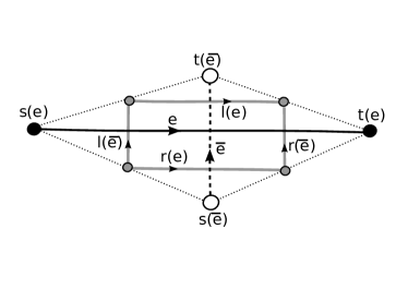
Figure 4: The four edges $r(e)$, $l(e)$, $r(\bar{e})$, $l(\bar{e})$ of ${\Gamma_{D}}$ for an edge $e$ of $\Gamma$.

Alternatively, the ribbon graph ${\Gamma_{D}}$ can also be obtained from the Poincaré dual. For this, one embeds $\Gamma$ into the oriented surface $\Sigma_{\Gamma}$ and considers its Poincaré dual $\bar{\Gamma}$. To construct ${\Gamma_{D}}$ one connects each vertex $v\in V(\Gamma)$ to those vertices $\bar{f}\in V(\bar{\Gamma})$ that are dual to faces containing $v$. By selecting a point in the interior of each of the resulting edges $e_{vf}$, one obtains the vertices of ${\Gamma_{D}}$. The edges of ${\Gamma_{D}}$ are obtained by connecting those vertices of ${\Gamma_{D}}$ for which the edges $e_{vf}$ and $e_{v^{\prime}f^{\prime}}$ are adjacent at a vertex of $\Gamma$ or at a dual vertex of $\bar{\Gamma}$. This construction is shown in Figure 5.

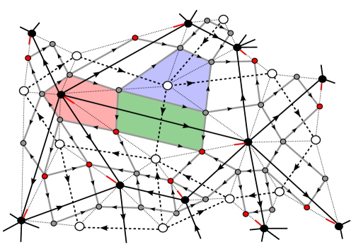
Figure 5: Ribbon graph $\Gamma$ (black vertices and black edges), its dual $\bar{\Gamma}$ (white vertices and dashed edges), the graph ${\Gamma_{D}}$ (grey and red vertices, grey edges). The cilia at the vertices of $\Gamma$ and the corresponding vertices of ${\Gamma_{D}}$ are indicated in red. The rectangle $R_{e}$ for an edge $e$ in $\Gamma$ is highlighted in green, the polygon $P_{v}$ for a vertex $v$ of $\Gamma$ in red and the polygon $P_{f}$ for a face $f$ of $\Gamma$ in blue.

The four edges of ${\Gamma_{D}}$ that correspond to a given edge $e$ of $\Gamma$ are denoted $r(e)$, $l(e)$, $r(\bar{e})$ and $l(\bar{e})$, where $r(e)$ and $l(e)$ stand for the edges of ${\Gamma_{D}}$ to the right and left of $e$, viewed in the direction of $e$. Similarly, $r(\bar{e})$, $l(\bar{e})$ are the edges of ${\Gamma_{D}}$ transversal to $e$ at the target and starting end of $e$, as shown in Figure 4. If $e\in E(\Gamma)$ and $\bar{e}\in E(\bar{\Gamma})$ are oriented edges and $e^{-1}$, $\bar{e}^{\,{-1}}$ the corresponding edges with the reversed orientation, then one has

$$r(e^{-1})=l(e)^{-1}\qquad r(\bar{e}^{-1})=l(\bar{e})^{-1}.$$ (17)

The four vertices of ${\Gamma_{D}}$ associated with a generic edge $e\in E(\Gamma)$ are given by the pairs $({\bf s}(e),{\bf s}(\bar{e}))$, $({\bf s}(e),{\bf t}(\bar{e}))$, $({\bf t}(e),{\bf s}(\bar{e}))$, $({\bf t}(e),{\bf t}(\bar{e}))$ where ${\bf s}(e)$ and ${\bf t}(e)$ are the starting and target vertex of $e$ and ${\bf s}(\bar{e})$ and ${\bf t}(\bar{e})$ the starting and target vertex of $\bar{e}$. More specifically, we have in ${\Gamma_{D}}$

$${\bf s}(r(\bar{e}))={\bf t}(r(e))=({\bf t}(e),{\bf s}(\bar{e})) {\bf t}(r(\bar{e}))={\bf t}(l(e))=({\bf t}(e),{\bf t}(\bar{e}))$$ (18)

$${\bf s}(l(\bar{e}))={\bf s}(r(e))=({\bf s}(e),{\bf s}(\bar{e})) {\bf t}(l(\bar{e}))={\bf s}(l(e))=({\bf s}(e),{\bf t}(\bar{e})),$$

as shown in Figure 4. Note that for edges of $\Gamma$ that are loops or dual to loops some of these four vertices may coincide, but this does not happen if $\Gamma$ is a regular ciliated ribbon graph. In this case the vertices of ${\Gamma_{D}}$ are in bijection with the sites of $\Gamma$ and each edge of $\Gamma$ corresponds to exactly four sites. The four vertices $s(e)$, $t(e)$, $s(\bar{e})$, $t(\bar{e})$ for an edge $e\in E(\Gamma)$ form four triangles, $s(e)s(\bar{e})t(\bar{e})$, $t(e)t(\bar{e})s(\bar{e})$, $t(e)t(\bar{e})s(e)$ and $t(e)s(e)s(\bar{e})$, which are called direct triangles and dual triangles in the context of Kitaev models, depending on their number of vertices and dual vertices.

Definition 5.1.

Let $\Gamma$ be a ribbon graph. The thickening of $\Gamma$ is the 4-valent ribbon graph ${\Gamma_{D}}$ with

$$E({\Gamma_{D}})=\cup_{e\in E(\Gamma)}\{r(e),l(e),r(\bar{e}),l(\bar{e})\}$$

$$V({\Gamma_{D}})=\cup_{e\in E(\Gamma)}\{({\bf s}(e),{\bf s}(\bar{e})),({\bf s}(e),{\bf t}(\bar{e})),({\bf t}(e),{\bf s}(\bar{e})),({\bf t}(e),{\bf t}(\bar{e}))\}\subset V(\Gamma)\times V(\bar{\Gamma}),$$

subject to the relations (18).

Note that a cilia of a ribbon graph $\Gamma$ can also be incorporated into the thickening ${\Gamma_{D}}$. Choosing a cilium at a vertex $v$ amounts to selecting a vertex of the polygon $P_{v}$ in the thickening ${\Gamma_{D}}$, namely the vertex of $P_{v}$ that is between the edge ends of highest and lowest order at $v$, as indicated in Figure 5. We will also call this vertex of ${\Gamma_{D}}$ the cilium at $v$ in the following.

5.2 Holonomies in the Kitaev model

Holonomies for a Kitaev model on $\Gamma$ are defined analogously to holonomies for a Hopf algebra gauge theory on $\Gamma$, but with respect to the thickened graph ${\Gamma_{D}}$ instead of $\Gamma$. As the algebra of triangle operators is isomorphic to the $E$-fold tensor product $\mathcal{H}(H)^{\otimes E}$ by Lemma 3.7 and $\mathcal{H}(H)\cong H\otimes H^{*}$ as a vector space, we define holonomy as a functor $\mathrm{Hol}:\mathcal{G}({\Gamma_{D}})\to\mathrm{Hom}_{\mathbb{F}}(H\otimes H^{*},(H\otimes H^{*})^{\otimes E})$, where $\mathcal{G}({\Gamma_{D}})$ is the path groupoid of ${\Gamma_{D}}$ and $\mathrm{Hom}_{\mathbb{F}}(H\otimes H^{*},(H\otimes H^{*})^{\otimes E})$ is equipped with the structure of an $\mathbb{F}$-linear category with a single object, i. e. an associative algebra structure over $\mathbb{F}$.

As in the case of a Hopf algebra gauge theory, this algebra structure is obtained from a coalgebra structure on $H\otimes H^{*}$ and an algebra structure on $(H\otimes H^{*})^{\otimes E}$ via (16). As $H\otimes H^{*}=D(H)^{*}$ as a vector space and to make contact with the holonomies in a Hopf algebra gauge theory for $D(H)$, it is natural to choose the coalgebra structure on $D(H)^{*}$ for the former and the canonical algebra structure on $D(H)^{*\otimes E}$ for the latter. As in the case of a Hopf algebra gauge theory, a holonomy functor is then determined uniquely by its values on the edges of ${\Gamma_{D}}$, i. e. by its values on the paths $r(e)^{\pm 1}$, $r(\bar{e})^{\pm 1}$, $l(e)^{\pm 1}$ and $l(\bar{e})^{\pm 1}$ for edges $e\in E(\Gamma)$. With the notation from Section 2.1 we obtain

Lemma 5.2.

Let $\Gamma$ be a ribbon graph with thickening ${\Gamma_{D}}$. Equip $\mathrm{Hom}_{\mathbb{F}}(H\otimes H^{*},(H\otimes H^{*})^{\otimes E})$ with the associative algebra structure $\bullet$ from (16) for the coalgebra $D(H)^{*}$ and the algebra $D(H)^{*\otimes E}$ and denote by $S_{D}:H\otimes H^{*}\to H\otimes H^{*}$ the antipode of $D(H)^{*}$. Then the following defines a functor $\mathrm{Hol}:\mathcal{G}({\Gamma_{D}})\to\mathrm{Hom}_{\mathbb{F}}(H\otimes H^{*},(H\otimes H^{*})^{\otimes E})$

$$\mathrm{Hol}_{r(e)}(y\otimes\gamma)=\epsilon(y)\,(1\otimes\gamma)_{e}\qquad\qquad\qquad\mathrm{Hol}_{r(\bar{e})}(y\otimes\gamma)=\epsilon(\gamma)(y\otimes 1)_{e},$$ (19)

$$\mathrm{Hol}_{l(e)}(y\otimes\gamma)=(S_{D}\circ\mathrm{Hol}_{r(e)}\circ S_{D})(y\otimes\gamma)=\epsilon(y)\Sigma_{i,j}(x_{i}S(x_{j})\otimes\alpha^{j}\gamma\alpha^{i})_{e}$$

$$\mathrm{Hol}_{l(\bar{e})}(y\otimes\gamma)=(S_{D}\circ\mathrm{Hol}_{r(\bar{e})}\circ S_{D})(y\otimes\gamma)=\epsilon(\gamma)\,\Sigma_{i,j}(x_{i}yS(x_{j})\otimes\alpha^{j}\alpha^{i})_{e}$$

$$\mathrm{Hol}_{x^{-1}}=\mathrm{Hol}_{x}\circ S_{D}\quad\forall x\in E({\Gamma_{D}}),e\in E(\Gamma).$$

Proof.

As $\mathcal{G}({\Gamma_{D}})$ is the free groupoid generated by $E({\Gamma_{D}})$, it is sufficient to show that for all $x\in E({\Gamma_{D}})$ one has $\mathrm{Hol}_{x}\bullet\mathrm{Hol}_{x^{-1}}=\mathrm{Hol}_{x^{-1}}\bullet\mathrm{Hol}_{x}=\epsilon\,(1\otimes 1)^{\otimes E}$ . The definition of $\bullet$ in (16) implies

$$\mathrm{Hol}_{x^{\pm 1}\circ x^{\mp 1}}(y\otimes\gamma) =\mathrm{Hol}_{x^{\pm 1}}((y\otimes\gamma)_{(1)})\cdot^{\prime}\mathrm{Hol}_{x^{\mp 1}}((y\otimes\gamma)_{(2)})$$ (20)

$$=\Sigma_{i,j}\,\mathrm{Hol}_{x^{\pm 1}}({y}_{({1})}\otimes\alpha^{i}{\gamma}_{({2})}\alpha^{j})\cdot^{\prime}\mathrm{Hol}_{x^{\mp 1}}(S(x_{j}){y}_{({2})}x_{i}\otimes{\gamma}_{({2})}),$$

where we use Sweedler notation and $\cdot^{\prime}$ denotes the multiplication of $D(H)^{*\otimes E}$. With the expression for $S_{D}$ in (2), one obtains from (19)

$$\mathrm{Hol}_{x^{-1}}(y\otimes\gamma)=\epsilon(y)\;\mathrm{Hol}_{x}(1\otimes S(\gamma))\;\;\forall x\in\{r(e),l(e)\}$$ (21)

$$\mathrm{Hol}_{x^{-1}}(y\otimes\gamma)=\epsilon(\gamma)\;\mathrm{Hol}_{x}(S(y)\otimes 1)\;\;\forall x\in\{\bar{r}(e),\bar{l}(e)\}.\qquad\qquad\qquad$$

Inserting this into (20) with the formulas in (2) for the multiplication and comultiplication of $D(H)^{*}$ and the identity $m\circ(S_{D}\otimes\mathrm{id})\circ\Delta=m\circ(\mathrm{id}\otimes S_{D})\circ\Delta=\epsilon\,1$ and $S^{2}_{D}=\mathrm{id}$ then proves the claim. ∎

Note that this is not the only possible holonomy functor since there is at least one other candidate for the multiplication on $(H\otimes H^{*})^{\otimes E}$ that enters the definition of $\bullet$ in (16), namely the multiplication map of $\mathcal{H}(H)^{\otimes E}$. However, the multiplication of $D(H)^{*\otimes E}$ is more natural from the viewpoint of Hopf algebra gauge theory. Defining the multiplication $\bullet$ in (16) with the comultiplication of $K^{*}$ and the multiplication of $K^{*\otimes E}$ is possible for any Hopf algebra $K$, while the multiplication of $\mathcal{H}(H)^{\otimes E}$ is only available for a Drinfeld double $K=D(H)$. Another strong motivation to choose the multiplication of $D(H)^{*\otimes E}$ are the properties of the resulting holonomy functor.

Lemma 5.3.

The holonomy functor from Lemma 5.2 satisfies:

1. $\mathrm{Hol}_{p}(1\otimes 1)=(1\otimes 1)^{\otimes E}$ for all paths $p$ in ${\Gamma_{D}}$.
   

2. $\mathrm{Hol}_{p^{-1}}=\mathrm{Hol}_{p}\circ S_{D}$ if $p$ is a path that traverses each edge of ${\Gamma_{D}}$ at most once and at most one of the edges $r(e)$, $l(e)$ and of the edges $r(\bar{e})$, $l(\bar{e})$ for each edge $e$ of $\Gamma$.
   

3. $\mathrm{Hol}_{p}(y\otimes\gamma)=\epsilon(y)\mathrm{Hol}_{p}(1\otimes\gamma)$ if $p$ is a path composed of edges $r(e),l(e)$ for edges $e$ of $\Gamma$.
   

4. $\mathrm{Hol}_{p}(y\otimes\gamma)=\epsilon(\gamma)\mathrm{Hol}_{p}(y\otimes 1)$ if $p$ is a path composed of the edges $r(\bar{e}),l(\bar{e})$ for edges $e$ of $\Gamma$.
   

5. $\mathrm{Hol}_{r(\bar{e})\circ r(e)}=\mathrm{Hol}_{l(e)\circ l(\bar{e})}$ and $\mathrm{Hol}_{r(\bar{e})^{-1}\circ l(e)}=\mathrm{Hol}_{r(e)\circ l(\bar{e})^{-1}}.$

Proof.

Claim 1. follows directly from the identities $\Delta(1\otimes 1)=(1\otimes 1)\otimes(1\otimes 1)$, $\epsilon(1)=1$ together with equation (19). Claims 2.-4. follow by induction over the length of $p$. If $p$ is a path of length 1, then they hold by definition. For a composite path $p\circ q$ one has

$$\mathrm{Hol}_{p\circ q}(y\otimes\gamma)=\mathrm{Hol}_{p}((y\otimes\gamma)_{(1)})\cdot^{\prime}\mathrm{Hol}_{q}((y\otimes\gamma)_{(2)})$$ (22)

$$\mathrm{Hol}_{(p\circ q)^{-1}}(y\otimes\gamma)=\mathrm{Hol}_{q^{-1}\circ p^{-1}}(y\otimes\gamma)=\mathrm{Hol}_{q^{-1}}((y\otimes\gamma)_{(1)})\cdot^{\prime}\mathrm{Hol}_{p^{-1}}((y\otimes\gamma)_{(2)}).$$

Suppose that 2. is shown for all paths of length $\leq n$. If $p\circ q$ is a path of length $n+1$ that satisfies the assumptions of 2., then so do $p$ and $q$. As they are of length $\leq n$, by induction hypothesis the last expression in (22) can be rewritten as

$$\mathrm{Hol}_{(p\circ q)^{-1}}(y\otimes\gamma)=\mathrm{Hol}_{q}(S_{D}(y\otimes\gamma)_{(2)})\cdot^{\prime}\mathrm{Hol}_{p}(S_{D}(y\otimes\gamma)_{(1)}),$$

where we used the identity $(S_{D}\otimes S_{D})\circ\Delta=\Delta^{op}\circ S_{D}$. If $p\circ q$ traverses each edge of ${\Gamma_{D}}$ at most once and at most one of the edges $r(e)$, $l(e)$ and of $r(\bar{e})$, $l(\bar{e})$ for each edge $e\in E(\Gamma)$ then the holonomies $\mathrm{Hol}_{q}(S_{D}(y\otimes\gamma)_{(2)})$ and $\mathrm{Hol}_{p}(S_{D}(y\otimes\gamma)_{(1)})$ commute in $D(H)^{*\otimes E}\cong(H^{op}\otimes H^{*})^{\otimes E}$, and one obtains

$$(\mathrm{Hol}_{p\circ q}\circ S_{D})(y\otimes\gamma)=\mathrm{Hol}_{p}(S_{D}(y\otimes\gamma)_{(1)})\cdot^{\prime}\mathrm{Hol}_{q}(S_{D}(y\otimes\gamma)_{(2)})=\mathrm{Hol}_{(p\circ q)^{-1}}(y\otimes\gamma).$$

Suppose that 3. is shown for all paths of length $\leq n$. If $p\circ q$ is a path of length $n+1$ that satisfies the assumptions in 3., then so do $p$ and $q$. By induction hypothesis this implies

$$\mathrm{Hol}_{p\circ q}(y\otimes\gamma)=\Sigma_{i,j}\,\mathrm{Hol}_{p}({y}_{({1})}\otimes\alpha^{i}{\gamma}_{({1})}\alpha^{j})\cdot^{\prime}\mathrm{Hol}_{q}(S(x_{j}){y}_{({2})}x_{i}\otimes{\gamma}_{({2})})$$

$$=\epsilon({y}_{({1})})\Sigma_{i,j}\,\epsilon(S(x_{j}){y}_{({2})}x_{i})\;\mathrm{Hol}_{p}(1\otimes\alpha^{i}{\gamma}_{({1})}\alpha^{j})\cdot^{\prime}\mathrm{Hol}_{q}(1\otimes{\gamma}_{({2})})$$

$$=\epsilon(y)\;\mathrm{Hol}_{p}(1\otimes{\gamma}_{({1})})\cdot^{\prime}\mathrm{Hol}_{q}(1\otimes{\gamma}_{({2})})=\epsilon(y)\Sigma_{i,j}\,\epsilon(x_{i}S(x_{j}))\mathrm{Hol}_{p}(1\otimes\alpha^{i}{\gamma}_{({1})}\alpha^{j})\cdot^{\prime}\mathrm{Hol}_{q}(1\otimes{\gamma}_{({2})})$$

$$=\epsilon(y)\mathrm{Hol}_{p}((1\otimes\gamma)_{(1)})\cdot^{\prime}\mathrm{Hol}_{q}((1\otimes{\gamma}_{({2})})_{(2)})=\epsilon(y)\mathrm{Hol}_{p\circ q}(1\otimes\gamma)$$

Suppose 4. holds for all paths of length $\leq n$. If $p\circ q$ is a path of length $n+1$ that satisfies the assumptions of 4., then so do $p$ and $q$. With the induction hypothesis one obtains

$$\mathrm{Hol}_{p\circ q}(y\otimes\gamma)=\Sigma_{i,j}\,\mathrm{Hol}_{p}({y}_{({1})}\otimes\alpha^{i}{\gamma}_{({1})}\alpha^{j})\cdot^{\prime}\mathrm{Hol}_{q}(S(x_{j}){y}_{({2})}x_{i}\otimes{\gamma}_{({2})})$$

$$=\Sigma_{i,j}\,\epsilon(\alpha^{i}{\gamma}_{({1})}\alpha^{j})\epsilon({\gamma}_{({2})})\;\mathrm{Hol}_{p}({y}_{({1})}\otimes 1)\cdot^{\prime}\mathrm{Hol}_{q}(S(x_{j}){y}_{({2})}x_{i}\otimes 1)$$

$$=\epsilon(\gamma)\;\mathrm{Hol}_{p}({y}_{({1})}\otimes 1)\cdot^{\prime}\mathrm{Hol}_{q}({y}_{({2})}\otimes 1)=\epsilon(\gamma)\Sigma_{i,j}\,\epsilon(\alpha^{i}\alpha^{j})\mathrm{Hol}_{p}({y}_{({1})}\otimes 1)\cdot^{\prime}\mathrm{Hol}_{q}(S(x_{j}){y}_{({2})}x_{i}\otimes 1)$$

$$=\epsilon(\gamma)\;\mathrm{Hol}_{p}((y\otimes 1)_{(1)})\cdot^{\prime}\mathrm{Hol}_{q}((y\otimes 1)_{(2)})=\epsilon(\gamma)\mathrm{Hol}_{p\circ q}(y\otimes 1).$$

To prove 5. we compute the holonomies using the expressions in Lemma 5.2, the expression for the comultiplication and antipode of $D(H)^{*}$ in (2) and the identities (9), (10) and (11). This yields

$$\mathrm{Hol}_{r(\bar{e})\circ r(e)}(y\otimes\gamma)=\Sigma_{i,j}\,\epsilon(\alpha^{i}{\gamma}_{({1})}\alpha^{j})\epsilon(S(x_{j}){y}_{({2})}x_{i})({y}_{({1})}\otimes 1)_{e}\cdot^{\prime}(1\otimes{\gamma}_{({2})})_{e}=(y\otimes\gamma)_{e},$$

$$\mathrm{Hol}_{l(e)\circ l(\bar{e})}(y\otimes\gamma)$$

$$=\epsilon({y}_{({1})})\epsilon({\gamma}_{({2})})\Sigma_{i,j,r,s,u,v}\,(x_{r}x_{s}\otimes S(\alpha^{s})\alpha^{i}{\gamma}_{({2})}\alpha^{j}\alpha^{r})_{e}\cdot^{\prime}(x_{u}S(x_{j}){y}_{({2})}x_{i}x_{v}\otimes S(\alpha^{v})\alpha^{u})_{e}$$

$$=\Sigma_{i,j,r,s,u,v}\,(x_{u}S(x_{j})yx_{i}x_{v}x_{r}x_{s}\otimes S(\alpha^{s})\alpha^{i}\gamma\alpha^{j}\alpha^{r}S(\alpha^{v})\alpha^{u})_{e}=(y\otimes\gamma)_{e},$$

$$\mathrm{Hol}_{r(\bar{e})^{-1}\circ l(e)}(y\otimes\gamma)$$

$$=\Sigma_{i,j,r,s,u,v}\,\epsilon(S(\alpha^{s})S(\alpha^{i}{\gamma}_{({1})}\alpha^{j})\alpha^{r})\epsilon(S(x_{j}){y}_{({2})}x_{i})(x_{r}S({y}_{({1})})x_{s}\otimes 1)_{e}\cdot^{\prime}(x_{u}x_{v}\otimes S(\alpha^{v}){\gamma}_{({2})}\alpha^{u})_{e}$$

$$=\Sigma_{u,v}\,(S(y)\otimes 1)_{e}\cdot^{\prime}(x_{u}x_{v}\otimes S(\alpha^{v})\gamma\alpha^{u})_{e}=\Sigma_{u,v}\,(x_{u}x_{v}S(y)\otimes S(\alpha^{v})\gamma\alpha^{u})_{e},$$

$$\mathrm{Hol}_{r(e)\circ l(\bar{e})^{-1}}(y\otimes\gamma)$$

$$=\epsilon({y}_{({1})})\Sigma_{i,j,r,s,u,v}\,\epsilon(S(\alpha^{s})S({\gamma}_{({2})})\alpha^{r})(1\otimes\alpha^{i}{\gamma}_{({1})}\alpha^{j})_{e}\cdot^{\prime}(x_{u}x_{s}S(S(x_{j}){y}_{({2})}x_{i})x_{r}x_{v}\otimes S(\alpha^{v})\alpha^{u})_{e}$$

$$=\Sigma_{i,j,u,v}\,(1\otimes\alpha^{i}\gamma\alpha^{j})_{e}\cdot^{\prime}(x_{u}S(x_{i})S(y)x_{j}x_{v}\otimes S(\alpha^{v})\alpha^{u})_{e}$$

$$=\Sigma_{i,j,u,v}\,(x_{u}S(x_{i})S(y)x_{j}x_{v}\otimes\alpha^{i}\gamma\alpha^{j}S(\alpha^{v})\alpha^{u})_{e}=\Sigma_{u,v}\,(x_{u}x_{v}S(y)\otimes S(\alpha^{v})\gamma\alpha^{u})_{e}.$$

∎

The identities in Lemma 5.3, 5. have a direct geometrical interpretation, shown in Figure 6. They state that for the rectangle $R_{e}$ associated to an edge $e\in E(\Gamma)$ the two paths from a vertex of $R_{e}$ to the diagonally opposite vertex have the same holonomy. In particular, this implies that the holonomies of two paths in ${\Gamma_{D}}$ that involve only the edges $r(e),l(e),r(\bar{e}),l(\bar{e})$ and their inverses agree whenever the paths have the same starting and target vertex. Had one defined the holonomy functor by expressions (19) but with the multiplication of $\mathcal{H}(H)^{\otimes E}$ instead of $D(H)^{*\otimes E}$ in (16), this result would not hold.

Although the choice of the multiplication of $D(H)^{*\otimes E}$ and the multiplication $\mathcal{H}(H)^{\otimes E}$ for the multiplication in (16) generally lead to different notions of holonomies, there is a class of paths for which the resulting holonomies agree. These are precisely the ribbon paths introduced in [28, 13], and their holonomies are the ribbon operators from [28, 13]. In a formulation adapted to our notation and conventions, ribbon paths are defined as follows.

Figure 6: The relations from Lemma 5.3, 5.

Definition 5.4.

A path $p\in\mathcal{G}({\Gamma_{D}})$ is called a ribbon path if it traverses each edge of ${\Gamma_{D}}$ at most once and for each edge $e\in E(\Gamma)$ traverses either edges in $\{r(e),l(e)\}$ or edges in $\{r(\bar{e}),l(\bar{e})\}$.

The name ribbon path is motivated by the fact that a ribbon path can be thickened to a ribbon on a surface by associating to each edge $x\in E({\Gamma_{D}})$ one of the four triangles in Figure 4 [28, 13], namely the triangle $s(e)s(\bar{e})t(\bar{e})$ to $l(\bar{e})$, the triangle $t(e)t(\bar{e})s(\bar{e})$ to $r(\bar{e})$, the triangle $t(e)t(\bar{e})s(e)$ to $l(e)$ and the triangle $t(e)s(e)s(\bar{e})$ to $r(\bar{e})$. If $p\in\mathcal{G}({\Gamma_{D}})$ is a ribbon path, then the triangles for edges in $p$ overlap only on their boundaries and thicken $p$ to a ribbon, as shown in Figure 7.

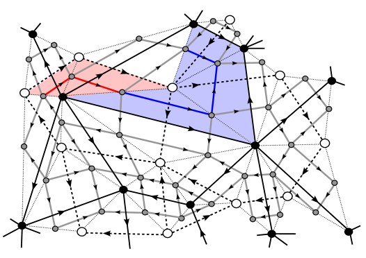
Figure 7: A ribbon graph in the thickened graph ${\Gamma_{D}}$ and its thickening by triangles. Edges of the form $r(\bar{e})^{\pm 1}$, $l(\bar{e})^{\pm 1}$ in the path and the associated triangles are indicated in red and edges of the form $r(e)^{\pm 1}$, $l(e)^{\pm 1}$ and the associated triangles in blue.

The ribbon operators from [28, 13, 15] associate to each element of $H\otimes H^{*}$ and each ribbon path $p\in\mathcal{G}({\Gamma_{D}})$ a linear map $H^{\otimes E}\to H^{\otimes E}$, which corresponds to a unique element of the algebra $\mathcal{H}(H)^{\otimes E}$ by Lemma 3.7. Hence, ribbon operators can be viewed as a linear map $H\otimes H^{*}\to(H\otimes H^{*})^{\otimes E}$. A close inspection of the formulas in [28, 13] show that this map is obtained by choosing the comultiplication of $D(H)^{*}$ and the multiplication of $\mathcal{H}(H)^{\otimes E}$ in (16). This is made explicit in [13] for the group algebra of a finite group and generalised implicitly in [15] to finite-dimensional semisimple Hopf algebras. It turns out that for ribbon paths that satisfy a mild additional assumption the two notions of holonomies agree and our notion of holonomy yields precisely the ribbon operators.

Lemma 5.5.

Let $p\in\mathcal{G}({\Gamma_{D}})$ be a ribbon path such that for every edge $e\in E(\Gamma)$ for which $p$ traverses both $r(e),l(e)\in E({\Gamma_{D}})$ the edge $r(e)$ is traversed first and for each edge $e\in E(\Gamma)$ for which $p$ traverses both $r(\bar{e}),l(\bar{e})\in E({\Gamma_{D}})$ the edge $r(\bar{e})$ is traversed first. Then the holonomies of $p$ with respect to the multiplication of $\mathcal{H}(H)^{\otimes E}$ and $D(H)^{*\otimes E}$ agree.

Proof.

We denote by $\cdot$ the multiplication of $\mathcal{H}(H)^{\otimes E}$ and by $\cdot^{\prime}$ the multiplication of $D(H)^{*\otimes E}$. Suppose that $p$ is given by a reduced word $p=x_{1}^{\epsilon_{1}}\circ...\circ x_{n}^{\epsilon_{n}}$ with $x_{i}\in E({\Gamma_{D}})$ and $\epsilon_{i}\in\{\pm 1\}$. Then the holonomy of $p$ with respect to the multiplication of $D(H)^{*\otimes E}$ takes the form

$$\mathrm{Hol}_{p}(y\otimes\gamma)=\mathrm{Hol}_{x_{1}^{\epsilon_{1}}}((y\otimes\gamma)_{(1)})\cdot^{\prime}....\cdot^{\prime}\mathrm{Hol}_{x_{n}^{\epsilon_{n}}}((y\otimes\gamma)_{(n)}),$$

and the expression for the holonomy of $p$ with respect to the multiplication of $\mathcal{H}(H)^{\otimes E}$ is obtained by replacing $\cdot^{\prime}$ with $\cdot$ in this expression. If $p$ is a ribbon path, then for each edge $e\in E({\Gamma_{D}})$ there are at most two distinct $i,j\in\{1,...,n\}$ with $x_{i},x_{j}\in\{r(e),l(e),r(\bar{e}),l(\bar{e})\}$, and if there are two of them, one has either $\{x_{i},x_{j}\}=\{r(e),l(e)\}$ or $\{x_{i},x_{j}\}=\{r(\bar{e}),l(\bar{e})\}$. Hence, the contribution of $\mathrm{Hol}_{p}(y\otimes\gamma)$ to the copy of $H\otimes H^{*}$ associated with an edge $e\in E(\Gamma)$ is one of the following

1. $\mathrm{Hol}_{x}(z\otimes\delta)$ with $z\in H$, $\delta\in H^{*}$ and $x\in\{r(e),l(e),r(\bar{e}),l(\bar{e})\}$ if $p$ traverses at most one of the edges $r(e),l(e),r(\bar{e}),l(\bar{e})$,
   

2. $\mathrm{Hol}_{l(e)}(x\otimes\beta)\cdot^{\prime}\mathrm{Hol}_{r(e)}(z\otimes\delta)$ with $x,z\in H$, $\beta,\delta\in H^{*}$ if $p$ traverses both $l(e)$ and $r(e)$,
   

3. $\mathrm{Hol}_{l(\bar{e})}(x\otimes\beta)\cdot^{\prime}\mathrm{Hol}_{r(\bar{e})}(z\otimes\delta)$ with $x,z\in H$, $\beta,\delta\in H^{*}$ if $p$ traverses both $l(\bar{e})$ and $r(\bar{e})$.

As the different copies of $H\otimes H^{*}$ on $(H\otimes H^{*})^{\otimes E}$ commute with respect to both $\cdot$ and $\cdot^{\prime}$, it is sufficient to consider the last two cases. For (ii) and (iii) one computes with (19), the expressions for the multiplication, comultiplication and antipode of $D(H)^{*}$ in (2), the multiplication of $\mathcal{H}(H)$ in (6) and with the identities (9) and (10)

$$\mathrm{Hol}_{l(e)}(x\otimes\beta)\cdot^{\prime}\mathrm{Hol}_{r(e)}(z\otimes\delta)=\epsilon(x)\epsilon(z)\Sigma_{i,j}\,(x_{i}S(x_{j})\otimes\alpha^{j}\beta\alpha^{i})_{e}\cdot^{\prime}(1\otimes\delta)_{e}$$

$$=\epsilon(x)\epsilon(z)\Sigma_{i,j}\,(x_{i}S(x_{j})\otimes\alpha^{j}\beta\alpha^{i}\delta)_{e}=\epsilon(x)\epsilon(z)\Sigma_{i,j}\,(x_{i}S(x_{j})\otimes\alpha^{j}\beta\alpha^{i})_{e}\cdot(1\otimes\delta)_{e}$$

$$=\mathrm{Hol}_{l(e)}(x\otimes\beta)\cdot\mathrm{Hol}_{r(e)}(z\otimes\delta)$$

$$\mathrm{Hol}_{l(\bar{e})}(x\otimes\beta)\cdot^{\prime}\mathrm{Hol}_{r(\bar{e})}(z\otimes\delta)=\epsilon(\beta)\epsilon(\gamma)\Sigma_{i,j}\,(x_{i}xS(x_{j})\otimes\alpha^{j}\alpha^{i})\cdot^{\prime}(z\otimes 1)$$

$$=\epsilon(\beta)\epsilon(\delta)\Sigma_{i,j}\,(zx_{i}xS(x_{j})\otimes\alpha^{j}\alpha^{i})=\epsilon(\beta)\epsilon(\delta)\Sigma_{i,j}\,(z_{(3)}x_{i}xS(x_{j})S(z_{(2)}){z}_{({1})}\otimes\alpha^{j}\alpha^{i})$$

$$=\epsilon(\beta)\epsilon(\delta)\Sigma_{i,j}\,\langle\alpha^{j}_{(1)}\alpha^{i}_{(1)},{z}_{({2})}\rangle(x_{i}xS(x_{j}){z}_{({1})}\otimes\alpha^{j}_{(2)}\alpha^{i}_{(2)})$$

$$=\epsilon(\beta)\epsilon(\delta)\Sigma_{i,j}\,(x_{i}xS(x_{j})\otimes\alpha^{j}\alpha^{i})\cdot(z\otimes 1)=\mathrm{Hol}_{l(\bar{e})}(x\otimes\beta)\cdot\mathrm{Hol}_{r(\bar{e})}(z\otimes\delta).$$

This shows that the holonomies of $p$ with respect to the multiplications $\cdot$ and $\cdot^{\prime}$ coincide. ∎

Although for ribbon paths the holonomies from Lemma 5.2 yield the ribbon operators from [28, 13, 15] and hence coincide with the notion of holonomy in the Kitaev models, the notion of holonomy in Lemma 5.2 is more conceptual. More importantly, it not restricted to ribbon paths but defined for any path $p$ in ${\Gamma_{D}}$ and hence more general than ribbon operators in Kitaev models. This will be essential when we relate the Kitaev models to a Hopf algebra gauge theory in Section 7. We will show that the relation between the two models is given by the holonomies of certain paths in ${\Gamma_{D}}$ that are not ribbon paths. The identity in Lemma 5.3, 5, which holds only if one defines holonomy with the multiplication of $D(H)^{*\otimes E}$ in (16), will be essential in establishing this relation.

5.3 Vertex and face operators

In this subsection we consider the holonomies of loops in the thickened ribbon graph ${\Gamma_{D}}$ that go clockwise around the vertices and faces of $\Gamma$ and relate them to the vertex and face operators in Kitaev models. We then determine the commutation relations of these holonomies and prove analogues of Lemma 3.3 and Lemma 3.4. As these loops are ribbon paths, this is essentially a rederivation of the results on vertex and face operators in [28, 13, 15], and readers familiar with them may skip this subsection. However, as we use a different notion of holonomy, with different conventions and build on these results in the following, it is necessary to derive them rigorously. Another reason to so is to make the paper self-contained and accessible to other communities.

Definition 5.6.

Let $\Gamma$ be ribbon graph without loops or multiple edges.

1. If $v$ is a ciliated vertex of $\Gamma$ with $n$ incident edges $e_{1},...,e_{n}$, numbered according to the ordering at $v$ and such that $e_{1}^{\epsilon_{1}}$,…,$e_{n}^{\epsilon_{n}}$ are incoming, then the vertex loop for $v$ is the path

   $$p_{v}=r(\bar{e}_{1}^{\epsilon_{1}})\circ\ldots\circ r(\bar{e}_{n}^{\epsilon_{n}})\in\mathcal{G}({\Gamma_{D}}),$$

2. If $f=e_{1}^{\epsilon_{1}}\circ\ldots\circ e_{n}^{\epsilon_{n}}$ is a ciliated face of $\Gamma$, then the associated face loop is the path

   $$p_{f}=r(e_{1}^{\epsilon_{1}})\circ\ldots\circ r(e_{n}^{\epsilon_{n}})\in\mathcal{G}({\Gamma_{D}}).$$

An example of a vertex loop is given in Figure 8 and an example of a face loop in Figure 9. Note that a vertex and face loops are in duality. A vertex loop $p_{v}$ for a ciliated vertex $v$ of $\Gamma$ can be viewed as a face loop for the associated ciliated face of the Poincaré dual $\bar{\Gamma}$. Similarly, a face loop $p_{f}$ for a ciliated face $f$ of $\Gamma$ corresponds to a vertex loop for the associated ciliated vertex of $\bar{\Gamma}$.

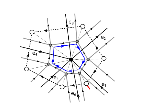
Figure 8: The vertex loop $p_{v}=r(\bar{e}_{1})\circ l(\bar{e}_{2})^{-1}\circ l(\bar{e}_{3})^{-1}\circ r(\bar{e}_{4})\circ r(\bar{e}_{5})\circ r(\bar{e}_{6}).$

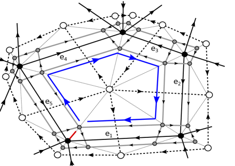
Figure 9: The face loop $p_{f}=r(e_{1})\circ r(e_{2})\circ l(e_{3})^{-1}\circ r(e_{4})\circ l(e_{5})^{-1}$ for $f=e_{1}\circ e_{2}\circ e_{3}^{-1}\circ e_{4}\circ e_{5}^{-1}$.

With the definition of the holonomies from Lemma 5.2, the correspondence between the holonomies of vertex and face loops and vertex and face operators requires mild additional assumptions that can be satisfied for any ciliated ribbon graph $\Gamma$ by reversing the orientations of certain edges. However, to keep the notation simple and because this is the only case required in the following, we restrict attention to ciliated ribbon graphs $\Gamma$ that satisfy the stronger regularity conditions in Definition 2.17. The holonomies of vertex and face loops are then mapped to the vertex and face operators from Definition 3.2 by the algebra isomorphism $\rho:\mathcal{H}(H)\to\mathrm{End}_{\mathbb{F}}(H^{\otimes E})$ from Lemma 3.7.

Lemma 5.7.

Let $\Gamma$ be a regular ciliated ribbon graph with thickening ${\Gamma_{D}}$. For every ciliated vertex $v$ and every ciliated face $f$ of $\Gamma$, the maps $\mathrm{Hol}_{p_{v}}|_{H}:H\to\mathcal{H}(H)^{\otimes E}$ and $\mathrm{Hol}_{p_{f}}|_{H^{*}}:H^{*}\to\mathcal{H}(H)^{\otimes E}$ are algebra morphisms and for all $y\in H$ and $\alpha\in H^{*}$ one has

$$\rho\circ\mathrm{Hol}_{p_{v}}(y\otimes\alpha)=\epsilon(\alpha)\,A_{v}^{y}\qquad\rho\circ\mathrm{Hol}_{p_{f}}(y\otimes\alpha)=\epsilon(y)\,B^{\alpha}_{f}.$$

Proof.

Throughout the proof let $\cdot$ be the multiplication of $\mathcal{H}(H)^{\otimes E}$. If $v$ is a ciliated vertex with incident edges $e_{1},...,e_{n}$, numbered according to the ordering at $v$ and such that $e_{1}^{\epsilon_{1}}$, …, $e_{n}^{\epsilon_{n}}$ are incoming at $v$, then the associated vertex loop $p_{v}$ from Definition 5.6 is given by $p_{v}=r(\bar{e}_{1}^{\epsilon_{1}})\circ\ldots\circ r(\bar{e}_{n}^{\epsilon_{n}}).$ Similarly, for a ciliated face $f=e_{1}^{\epsilon_{1}}\circ\ldots\circ e_{n}^{\epsilon_{n}}$ the associated face loop from Definition 5.6 is given by $p_{f}=r(e_{1}^{\epsilon_{1}})\circ\ldots\circ r(e_{n}^{\epsilon_{n}})$, both subject to convention (17). By Lemma 5.5 their holonomies are

$$\mathrm{Hol}_{p_{v}}(y\otimes\alpha)=\epsilon(\alpha)\,\mathrm{Hol}_{r(\bar{e}_{1}^{\epsilon_{1}})}({y}_{({1})}\otimes 1)\cdot...\cdot\mathrm{Hol}_{r(\bar{e}_{n}^{\epsilon_{n}})}({y}_{({n})}\otimes 1)$$ (23)

$$\mathrm{Hol}_{p_{f}}(y\otimes\alpha)=\epsilon(y)\,\mathrm{Hol}_{r(e_{1}^{\epsilon_{1}})}(1\otimes{\alpha}_{({1})})\cdot...\cdot\mathrm{Hol}_{r(e_{n}^{\epsilon_{n}})}(1\otimes{\alpha}_{({n})}),$$

and with Definition 3.1 and Lemma 3.7 this yields

$$\rho\circ\mathrm{Hol}_{r(\bar{e}_{i}^{\epsilon_{i}})}(y\otimes 1)=\begin{cases}L^{y}_{e_{i},+}&\epsilon_{i}=1\\ L^{S(y)}_{e_{i},-}&\epsilon_{i}=-1,\end{cases}\qquad\rho\circ\mathrm{Hol}_{r(e_{i}^{\epsilon_{i}})}(1\otimes\alpha)=\begin{cases}T^{\alpha}_{e_{i},+}&\epsilon_{i}=1\\ T^{S(\alpha)}_{e_{i},-}&\epsilon_{i}=-1.\end{cases}$$ (24)

By applying the algebra isomorphism $\rho:\mathcal{H}(H)^{\otimes E}\to\mathrm{End}_{\mathbb{F}}(H^{\otimes E})$ from Lemma 3.7 to (23) and inserting (24) one obtains the operators $A^{y}_{v}$, $B^{\alpha}_{f}$ from Definition 3.2. That $\mathrm{Hol}_{p_{v}}|_{H}:H\to\mathcal{H}(H)^{\otimes E}$ is an algebra morphism follows from (23), because one has $\bar{e}_{i}\neq\bar{e}_{j}$ for $i\neq j$ by the assumptions on $\Gamma$ and hence the holonomy of $r(\bar{e}_{i}^{\epsilon_{i}})$ commutes with the holonomy of $r(\bar{e}_{j}^{\epsilon_{j}})$ for $i\neq j$. From (19) one has $\mathrm{Hol}_{r(\bar{e}_{i}^{\epsilon_{i}})}(y\otimes 1)\cdot\mathrm{Hol}_{r(\bar{e}_{i}^{\epsilon_{i}})}(z\otimes 1)=\mathrm{Hol}_{r(\bar{e}_{i}^{\epsilon_{i}})}(yz\otimes 1)$ for all $y,z\in H$. Similarly, the assumptions on $\Gamma$ imply that $e_{i}\neq e_{j}$ for all $i\neq j$ and hence the holonomy of $r({e_{i}}^{\epsilon_{i}})$ commutes with the holonomy of $r({e_{j}}^{\epsilon_{j}})$ for $i\neq j$. Formula (19) implies $\mathrm{Hol}_{r({e_{i}}^{\epsilon_{i}})}(1\otimes\alpha)\cdot\mathrm{Hol}_{r({e_{i}}^{\epsilon_{i}})}(1\otimes\beta)=\mathrm{Hol}_{r({e_{i}}^{\epsilon_{i}})}(1\otimes\alpha\beta)$ for all $\alpha,\beta\in H^{*}$, and it follows that $\mathrm{Hol}_{p_{f}}|_{H^{*}}:H^{*}\to\mathcal{H}(H)^{\otimes E}$ is an algebra morphism. ∎

We now consider the algebraic properties of the holonomies of vertex and face loops with respect to the algebra structure of $\mathcal{H}(H)^{\otimes E}$ and prove analogues of Lemma 3.3 and Lemma 3.4. This requires the following technical lemma.

Lemma 5.8.

Let $\Gamma$ be a regular ciliated ribbon graph and $v$ a vertex with $n$ incoming edges $e_{1},...,e_{n}$, numbered according to the ordering at $v$. Then the holonomies of the path $l(e_{i+1})^{-1}\circ r(e_{i})$ commute with the holonomies of the paths $r(e_{i+1})$, $l(e_{i})$ and $r(\bar{e}_{i})\circ r(\bar{e}_{i+1})$.

Proof.

We denote by $\cdot$ the multiplication of $\mathcal{H}(H)^{\otimes E}$ and by $\cdot^{\prime}$ the multiplication of $D(H)^{*\otimes E}$. That $\mathrm{Hol}_{l(e_{i+1}^{-1})\circ r(e_{i})}(z\otimes\beta)$ commutes with $\mathrm{Hol}_{r(e_{i+1})}(y\otimes\alpha)$ and with $\mathrm{Hol}_{l(e_{i})}(y\otimes\alpha)$ for all $y,z\in H$ and $\alpha,\beta\in H^{*}$ follows from the definition of the holonomy functor and the fact that for all $e\in E(\Gamma)$ the holonomies of $r(e)$ and $l(e)$ commute, which is a consequence of their definition in (19) and the identities in (7). To prove that the holonomy of $l(e_{i+1}^{-1})\circ r(e_{i})$ commutes with the holonomy of $r(\bar{e}_{i})\circ r(\bar{e}_{i+1})$, we compute with the multiplication law (6) of the Heisenberg double

$$\mathrm{Hol}_{l(e_{i+1})^{-1}\circ r(e_{i})}(z\otimes\beta)\cdot\mathrm{Hol}_{r(\bar{e}_{i})\circ r(\bar{e}_{i+1})}(y\otimes\alpha)$$

$$=\epsilon(z)\epsilon(\alpha)\;(x_{k}x_{l}\otimes S(\alpha^{l})S({\beta}_{({1})})\alpha^{k})_{e_{i+1}}\cdot(1\otimes{\beta}_{({2})})_{e_{i}}\cdot({y}_{({1})}\otimes 1)_{e_{i}}\cdot({y}_{({2})}\otimes 1)_{e_{i+1}}$$

$$=\epsilon(z)\epsilon(\alpha)\;\langle S(\alpha^{l}_{(2)})S({\beta}_{({2})})\alpha^{k}_{(1)},{y}_{({4})}\rangle\langle{\beta}_{({3})},{y}_{({2})}\rangle\;(x_{k}x_{l}{y}_{({3})}\otimes S(\alpha^{l}_{(1)})S({\beta}_{({1})})\alpha^{k}_{(2)})_{e_{i+1}}\cdot({y}_{({2})}\otimes{\beta}_{({4})})_{e_{i}}$$

$$=\epsilon(z)\epsilon(\alpha)\;\langle S({\beta}_{({2})}),{y}_{({5})}\rangle\langle{\beta}_{({3})},{y}_{({2})}\rangle\;({y}_{({6})}x_{k}x_{l}S({y}_{({4})}){y}_{({3})}\otimes S(\alpha^{l})S({\beta}_{({1})})\alpha^{k})_{e_{i+1}}\cdot({y}_{({2})}\otimes{\beta}_{({4})})_{e_{i}}$$

$$=\epsilon(z)\epsilon(\alpha)\;\langle S({\beta}_{({2})}),{y}_{({3})}\rangle\langle{\beta}_{({3})},{y}_{({2})}\rangle\;({y}_{({4})}x_{k}x_{l}\otimes S(\alpha^{l})S({\beta}_{({1})})\alpha^{k})_{e_{i+1}}\cdot({y}_{({2})}\otimes{\beta}_{({4})})_{e_{i}}$$

$$=\epsilon(z)\epsilon(\alpha)\;({y}_{({2})}x_{k}x_{l}\otimes S(\alpha^{l})S({\beta}_{({1})})\alpha^{k})_{e_{i+1}}\cdot({y}_{({1})}\otimes{\beta}_{({2})})_{e_{i}}$$

$$=\epsilon(z)\epsilon(\alpha)\;({y}_{({1})}\otimes 1)_{e_{i}}\cdot({y}_{({2})}\otimes 1)_{e_{i+1}}\cdot(x_{k}x_{l}\otimes S(\alpha^{l})S({\beta}_{({1})})\alpha^{k})_{e_{i+1}}\cdot(1\otimes{\beta}_{({2})})_{e_{i+1}}$$

$$=\mathrm{Hol}_{r(\bar{e}_{i})\circ r(\bar{e}_{i+1})}(y\otimes\alpha)\cdot\mathrm{Hol}_{l(e_{i+1})^{-1}\circ r(e_{i})}(z\otimes\beta).$$

Note that we replaced the multiplication of $D(H)^{*\otimes E}$ by the multiplication of $\mathcal{H}(H)^{\otimes E}$ in the expressions for the holonomies of $l(e_{i+1}^{-1})\circ r(e_{i})$ and $r(\bar{e}_{i})\circ r(\bar{e}_{i+1})$ because the paths $l(e_{i+1}^{-1})\circ r(e_{i})$ and $r(\bar{e}_{i})\circ r(\bar{e}_{i+1})$ satisfy the assumptions of Lemma 5.5. ∎

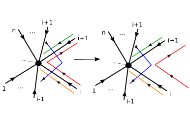
Figure 10: The paths from Lemma 5.8 and the Reidemeister II move at the vertex:
$l(e_{i+1})^{-1}\circ r(e_{i})$ (red), $r(\bar{e}_{i})\circ r(\bar{e}_{i+1})$ (blue), $l(e_{i})$ (orange) and $r(e_{i+1})$ (green).

The identities in Lemma 5.8 have a natural geometrical interpretation. They state that the holonomies of non-intersecting paths in ${\Gamma_{D}}$ commute and that an analogue of the Reidemeister II move can be used to remove intersection points of the paths $l(e_{i+1}^{-1})\circ r(e_{i})$ and $r(\bar{e}_{i})\circ r(\bar{e}_{i+1})$.

Lemma 5.9 (see Lemma 3.4).

Let $\Gamma$ be a regular ciliated ribbon graph, $v,v^{\prime}$ be two distinct vertices of $\Gamma$ and $f,f^{\prime}$ two ciliated faces that start and end at different cilia of $\Gamma$. Then:

1. The holonomies of the vertex loops $p_{v}$ and $p_{v^{\prime}}$ commute,

2. The holonomies of the face loops $p_{f}$ and $p_{f^{\prime}}$ commute,

3. If the cilium of $f$ does not coincide with the cilium at $v$, the holonomies of $p_{v}$ and $p_{f}$ commute.

Proof.

   
1. The vertex loop $p_{v}$ is composed of the paths $r(\bar{g})$ for edges $g\in E(\Gamma)$ with ${\bf t}(g)=v$ and of paths $l(\bar{g})^{-1}$ for edges $g\in E(\Gamma)$ with ${\bf s}(g)=v$. If $g\in E(\Gamma)$ is incident at $v$ but not at $v^{\prime}$ then the holonomies of $r(\bar{g})$ and $l(\bar{g})^{-1}$ commute with the holonomy of $p_{v^{\prime}}$. If $g\in E(\Gamma)$ is incident at both $v$ and $v^{\prime}$, we can suppose without restriction of generality that ${\bf t}(g)=v$ and ${\bf s}(g)=v^{\prime}$. Then $p_{v}$ contains only factors of the form $r(\bar{g})$ and $r(\bar{h})$, $l(\bar{h})^{-1}$ for edges $h\neq g$, and $p_{v^{\prime}}$ contains only factors of the form $l(\bar{g})^{-1}$ and $r(\bar{h})$, $l(\bar{h})^{-1}$ for edges $h\neq g$. The holonomies of $r(\bar{g})$ and $l(\bar{g})^{-1}$ commute with the holonomies of $r(\bar{h})$, $l(\bar{h})^{-1}$ for $h\neq g$, and by (7) they commute with each other. Hence, the holonomies of $p_{v}$ and $p_{v^{\prime}}$ commute.

2. If $f,f^{\prime}$ are ciliated faces of $\Gamma$ that start and end at different cilia of $\Gamma$, they are non-equivalent. For any edge $g\in E(\Gamma)$ that is traversed by both $f$ and $f^{\prime}$ either $p_{f}$ contains a factor $r(g)$ and $p_{f^{\prime}}$ contains a factor $l(g)$ or vice versa. The holonomies of $r(g)$ and $l(g)$ commute by (19) and (7). As the holonomies of $r(g)$ and $l(g)$ also commute with the holonomies of $r(h)$ and $l(h)$ for all edges $h\neq g$, the holonomies of $p_{f}$ and $p^{\prime}_{f}$ commute.

3. As $f$ starts and ends at a cilium and $\Gamma$ is regular, the face loop $p_{f}$ can be decomposed into paths $q$ that do not traverse any edges incident at $v$ and into paths of the form $r(\bar{f}^{\pm 1})\circ r(\bar{g}^{\pm 1})$, where $f$, $g$ are adjacent edges at $v$ with $g<f$. The holonomies of the former commute with the holonomy of $p_{v}$ by definition and the holonomies of the latter by Lemma 5.8 because $\mathrm{Hol}_{r(\bar{f}^{-1})}=\mathrm{Hol}_{l(\bar{f})^{-1}}=S_{D}\circ\mathrm{Hol}_{r(\bar{f})}$, $\mathrm{Hol}_{r(f^{-1})}=\mathrm{Hol}_{l(f)^{-1}}=S_{D}\circ\mathrm{Hol}_{r(f)}$ and $S_{D}:\mathcal{H}(H)\to\mathcal{H}(H)$ is an algebra homomorphism by Lemma 2.13. Hence, the holonomies of $p_{v}$ and $p_{f}$ commute. ∎

Lemma 5.10 (see Lemma 3.3).

Let $\Gamma$ be a regular ciliated ribbon graph. Denote for each vertex $v$ by $f(v)$ the ciliated face that starts and ends at the cilium at $v$. Then one obtains an algebra homomorphism

$$\tau:D(H)^{\otimes V}\to\mathcal{H}(H)^{\otimes E},\quad(\delta\otimes z)_{v}\mapsto\mathrm{Hol}_{p_{f(v)}}(1\otimes\delta)\cdot\mathrm{Hol}_{p_{v}}(z\otimes 1).$$ (25)

Proof.

By Lemma 5.10 the holonomies of $p_{v}$ and $p_{f(v)}$ commute with the holonomies of $p_{w}$ and $p_{f(w)}$ for all vertices $w\neq v$. Hence it is sufficient to show that for each vertex $v$ the linear map

$$\tau_{v}=\tau\circ\iota_{v}:D(H)\to\mathcal{H}(H)^{\otimes E},\quad\delta\otimes z\mapsto\mathrm{Hol}_{p_{f(v)}}(1\otimes\delta)\cdot\mathrm{Hol}_{p_{v}}(z\otimes 1)$$ (26)

is an algebra morphism. For this, let $v$ be a vertex with $n$ incident edges $e_{1},...,e_{n}$, numbered according to the ordering at $v$. As $\Gamma$ is loop-free and the map $S_{D}:\mathcal{H}(H)\to\mathcal{H}(H)$ is an algebra isomorphism by Lemma 2.13, we can suppose without loss of generality that all edges are incoming. Then the vertex loop $p_{v}$ is given by $p_{v}=r(\bar{e}_{1})\circ\ldots\circ r(\bar{e}_{n})$ and the associated face loop is of the form $p_{f(v)}=r(e_{n})\circ q\circ l(e_{1})^{-1}$, where $q$ is a path that turns maximally right at each vertex, traverses each edge at most once and does not traverse any cilia. This implies that $q$ can be decomposed into paths that do not traverse any edges incident at $v$ and paths of the form $r(g^{\pm 1})\circ r(h^{\pm 1})$ where $g,h$ are adjacent edges at $v$ with $h<g$. The holonomies of the former commute with the holonomy of $p_{v}$ by (19) and the holonomies of the latter by Lemma 5.8. This implies that the holonomy of $q$ commutes with the holonomy of $p_{v}$. As the maps $\mathrm{Hol}_{p_{v}}|_{H}:H\to\mathcal{H}(H)^{\otimes E}$ and $\mathrm{Hol}_{p_{f(v)}}|_{H^{*}}:H^{*}\to\mathcal{H}(H)^{\otimes E}$ are algebra homomorphisms by Lemma 5.7, we obtain

$$\mathrm{Hol}_{p_{f(v)}}(1\otimes\delta)\cdot\mathrm{Hol}_{p_{v}}(1\otimes z)=(1\otimes{\delta}_{({1})})_{e_{n}}\cdot\mathrm{Hol}_{q}(1\otimes{\delta}_{({2})})\cdot(x_{k}x_{l}\otimes S(\alpha^{l})S({\delta}_{({3})})\alpha^{k})_{e_{1}}\cdot\mathrm{Hol}_{p_{v}}(z\otimes 1)$$

$$=\langle S({\delta}_{({4})}),{z}_{({1})}\rangle\;(1\otimes{\delta}_{({1})})_{e_{n}}\cdot\mathrm{Hol}_{q}(1\otimes{\delta}_{({2})})\cdot\mathrm{Hol}_{p_{v}}(1\otimes{z}_{({2})})\cdot(x_{k}x_{l}\otimes S(\alpha^{l})S({\delta}_{({3})})\alpha^{k})_{e_{1}}$$

$$=\langle S({\delta}_{({5})}),{z}_{({1})}\rangle\langle{\delta}_{({1})},{z}_{({3})}\rangle\;\mathrm{Hol}_{p_{v}}(1\otimes{z}_{({2})})\cdot(1\otimes{\delta}_{({2})})_{e_{n}}\cdot\mathrm{Hol}_{q}(1\otimes{\delta}_{({3})})\cdot(x_{k}x_{l}\otimes S(\alpha^{l})S({\delta}_{({4})})\alpha^{k})_{e_{1}}$$

$$=\langle S({\delta}_{({3})}),{z}_{({1})}\rangle\langle{\delta}_{({1})},{z}_{({3})}\rangle\;\mathrm{Hol}_{p_{v}}(1\otimes{z}_{({2})})\cdot\mathrm{Hol}_{p_{f(v)}}(1\otimes{\delta}_{({2})}).$$

This implies for all $y,z\in H$ and $\gamma,\delta\in H^{*}$

$$\mathrm{Hol}_{p_{v}}(1\otimes z)\cdot\mathrm{Hol}_{p_{f(v)}}(1\otimes\delta)=\langle{\delta}_{({3})},{z}_{({1})}\rangle\langle{\delta}_{({1})},S({z}_{({3})})\rangle\;\mathrm{Hol}_{p_{f(v)}}(1\otimes{\delta}_{({2})})\cdot\mathrm{Hol}_{p_{v}}(1\otimes{z}_{({2})}).$$

A comparison with the multiplication of $D(H)$ in (1) then proves the claim. ∎

6 Gauge symmetries and flatness in Kitaev models

6.1 Gauge symmetries and gauge invariance

As explained in Section 4, the essential algebraic structure in a Hopf algebra gauge theory is the module algebra of functions over the Hopf algebra of gauge transformations. In this section we show that the Hopf algebra of gauge transformations in a Kitaev model is the $V$-fold tensor product $D(H)^{\otimes V}$ and the algebra $\mathcal{H}(H)^{op\otimes E}$ of triangle operators can be given the structure of a module algebra over this Hopf algebra. We can thus interpret $D(H)^{\otimes V}$ as a gauge symmetry of the Kitaev model similar to the gauge symmetries in a Hopf algebra gauge theory and obtain an associated subalgebra $\mathcal{H}(H)^{op\otimes E}_{inv}$ of invariants or gauge invariant observables.

In Section 6.2 we investigate the notion of curvature in Kitaev models and show that only those faces of ${\Gamma_{D}}$ that correspond to vertices and faces of $\Gamma$ give rise to curvatures. We then construct a subalgebra $\mathcal{H}(H)^{op\otimes E}_{flat}$ that can be viewed as the algebra of gauge invariant functions of flat gauge fields and acts on the protected space.

The $D(H)^{\otimes V}$- right module structure on Kitaev’s triangle operator algebra is induced by the algebra homomorphism (25), i. e. by the holonomies of the vertex and face loop based at a cilium of $\Gamma$.

Theorem 6.1.

Let $\Gamma$ be a regular ciliated ribbon graph. Denote for each vertex $v$ of $\Gamma$ by $f(v)$ the ciliated face that starts and ends at the cilium at $v$. Then $\lhd:\mathcal{H}(H)^{\otimes E}\otimes D(H)^{\otimes V}\to\mathcal{H}(H)^{\otimes E}$

$$X\lhd(\delta\otimes z)_{v} =\mathrm{Hol}_{p_{v}}(S({z}_{({2})})\otimes 1)\cdot\mathrm{Hol}_{p_{f(v)}}(1\otimes S({\delta}_{({1})}))\cdot X\cdot\mathrm{Hol}_{p_{f(v)}}(1\otimes{\delta}_{({2})})\cdot\mathrm{Hol}_{p_{v}}({z}_{({1})}\otimes 1)$$

$$=(\tau_{v}\circ S)((\delta\otimes z)_{(2)})\cdot X\cdot\tau_{v}((\delta\otimes z)_{(1)})$$ (27)

defines a $D(H)^{\otimes V}$-right module algebra structure on $\mathcal{H}(H)^{op\otimes E}$.

Proof.

It follows by a direct computation that for any Hopf algebra $K$, any algebra $A$ and any algebra homomorphism $\tau:K\to A$ the linear map $\lhd:A\otimes K\to A$, $a\lhd k=\tau(S({k}_{({2})}))\cdot a\cdot\tau({k}_{({1})})$ equips $A^{op}$ with the structure of a $K$-right module algebra. As the linear map $\tau:D(H)^{\otimes V}\to\mathcal{H}(H)^{\otimes E}$ is an algebra homomorphism by Lemma 5.10, the claim follows. ∎

As the $D(H)^{\otimes V}$-right module structure from Theorem 6.1 gives $\mathcal{H}(H)^{op\otimes E}$ the structure of a $D(H)^{\otimes V}$-module algebra, Lemma 2.6 defines a projector on its subalgebra of invariants. As $H$, $H^{*}$ and $D(H)$ are semisimple and $\text{char}(\mathbb{F})=0$, all tensor products of these Hopf algebras over $\mathbb{F}$ are semisimple as well and hence equipped with Haar integrals. If $\ell\in H$ and $\eta\in H^{*}$ denote the Haar integrals of $H$ and $H^{*}$, then $\eta\otimes\ell\in H^{*}\otimes H$ is the Haar integral for $D(H)$ and $(\eta\otimes\ell)^{\otimes V}$ the Haar integral for $D(H)^{\otimes V}$. By inserting the latter into the $D(H)^{\otimes V}$-module structure from Theorem 6.1 one obtains a projector on the gauge invariant subalgebra.

Lemma 6.2.

Let $\Gamma$ be a regular ciliated ribbon graph and $H$ a finite-dimensional semisimple Hopf algebra. Consider the $D(H)^{\otimes V}$-right module algebra structure on $\mathcal{H}(H)^{op\otimes E}$ from Theorem 6.1.

1. The linear map $Q_{inv}:\mathcal{H}(H)^{\otimes E}\to\mathcal{H}(H)^{\otimes E}$, $X\mapsto X\lhd(\eta\otimes\ell)^{\otimes V}$ is a projector.
   

2. Its image $\mathcal{H}(H)^{\otimes E}_{inv}=Q_{inv}(\mathcal{H}(H)^{\otimes E})$ is a subalgebra of $\mathcal{H}(H)^{\otimes E}$.
   

3. For all vertices $v$ the maps $Q_{inv}\circ\mathrm{Hol}_{p_{v}}$ and $Q_{inv}\circ\mathrm{Hol}_{p_{f(v)}}$ take values in the centre of $\mathcal{H}(H)^{\otimes E}_{inv}$.

Proof.

That $Q_{inv}$ is a projector and $Q_{inv}(\mathcal{H}(H)^{\otimes E})$ a subalgebra of $\mathcal{H}(H)^{\otimes E}$ follows with Lemma 2.6 and Lemma 2.10, because $(\eta\otimes\ell)^{\otimes V}$ is a Haar integral for $D(H)^{\otimes V}$ and $\mathcal{H}(H)^{op\otimes E}$ a $D(H)^{\otimes V}$-right module algebra by Theorem 6.1. To prove the third claim, note first that $(\eta\otimes 1)\cdot(1\otimes\ell)=(1\otimes\ell)\cdot(\eta\otimes 1)$ in $D(H)$, which follows directly from formula (1) for the multiplication of $D(H)$ and the cyclic invariance of $\Delta^{(3)}(\ell)$ and $\Delta^{(3)}(\eta)$. This implies for all vertices $v$ of $\Gamma$

$$\mathrm{Hol}_{p_{v}}(y\otimes\gamma)\lhd_{v}(\eta\otimes\ell)= \epsilon(\gamma)\,\mathrm{Hol}_{p_{v}}(S({\ell}_{({2})})y{\ell}_{({1})}\otimes 1)\lhd(\eta\otimes 1)_{v}$$ (28)

$$\mathrm{Hol}_{p_{f(v)}}(y\otimes\gamma)\lhd_{v}(\eta\otimes\ell)= \epsilon(y)\,\mathrm{Hol}_{p_{f(v)}}(1\otimes S({\eta}_{({1})})\gamma{\eta}_{({2})})\lhd(1\otimes\ell)_{v}.$$

As $S({\ell}_{({1})})\otimes{\ell}_{({2})}$ and $S({\eta}_{({1})})\otimes{\eta}_{({2})}$ are separability idempotents for $H$ and $H^{*}$ and $(1\otimes\ell)$ and $(\eta\otimes 1)$ commute in $D(H)$ we obtain from the $D(H)^{\otimes V}$-right module structure of $\mathcal{H}(H)^{\otimes E}$

$$(\mathrm{Hol}_{p_{v}}(y\otimes\gamma)\lhd(\eta\otimes\ell)_{v})\cdot(X\lhd(\eta^{\prime}\otimes\ell^{\prime})_{v})$$

$$=\epsilon(\gamma)\,\tau_{v}((S({\eta}_{({1})})\otimes 1)\cdot(1\otimes S({\ell}_{({2})})y{\ell}_{({1})})\cdot({\eta}_{({2})}S({\eta^{\prime}}_{({1})})\otimes 1))\cdot(X\lhd(1\otimes\ell^{\prime})_{v})\cdot\tau_{v}({\eta^{\prime}}_{({2})}\otimes 1)$$

$$=\epsilon(\gamma)\,\tau_{v}((S({\eta}_{({1})})\otimes 1)\cdot(1\otimes S({\ell}_{({2})})y{\ell}_{({1})})\cdot(S({\eta^{\prime}}_{({1})})\otimes 1))\cdot(X\lhd(\ell^{\prime}\otimes 1)_{v})\cdot\tau_{v}({\eta^{\prime}}_{({2})}{\eta}_{({2})}\otimes 1)$$

$$=\epsilon(\gamma)\,\tau_{v}((S({\eta}_{({1})})\otimes 1)\cdot(1\otimes S({\ell}_{({2})})y{\ell}_{({1})}S({\ell^{\prime}}_{({2})})))\cdot(X\lhd(\eta^{\prime}\otimes 1)_{v})\cdot\tau_{v}((1\otimes{\ell^{\prime}}_{({1})})\cdot({\eta}_{({2})}\otimes 1))$$

$$=\epsilon(\gamma)\,\tau_{v}((S({\eta}_{({1})})\otimes 1)\cdot(1\otimes S({\ell^{\prime}}_{({2})})))\cdot(X\lhd(\eta^{\prime}\otimes 1)_{v})\cdot\tau_{v}(1\otimes{\ell^{\prime}}_{({1})}S({\ell}_{({2})})y{\ell}_{({1})})\cdot\tau_{v}({\eta}_{({2})}\otimes 1)$$

$$=\epsilon(\gamma)\,\tau_{v}(S({\eta}_{({1})}S({\eta^{\prime}}_{({1})})\otimes 1)\cdot(X\lhd(1\otimes\ell^{\prime})_{v})\cdot\tau_{v}(({\eta^{\prime}}_{({2})}\otimes 1)\cdot(1\otimes S({\ell}_{({2})})y{\ell}_{({1})})\cdot({\eta}_{({2})}\otimes 1))$$

$$=\epsilon(\gamma)\,\tau_{v}(S({\eta^{\prime}}_{({1})})\otimes 1)\cdot(X\lhd(1\otimes\ell^{\prime})_{v})\cdot\tau_{v}(({\eta^{\prime}}_{({2})}S({\eta}_{({1})})\otimes 1)\cdot(1\otimes S({\ell}_{({2})})y{\ell}_{({1})})\cdot({\eta}_{({2})}\otimes 1))$$

$$=(X\lhd(\eta^{\prime}\otimes\ell^{\prime})_{v})\cdot(\mathrm{Hol}_{p_{v}}(y\otimes\gamma)\lhd(\eta\otimes\ell)_{v})$$

for all $y\in H$, $\gamma\in H^{*}$ and $X\in\mathcal{H}(H)^{\otimes E}$. As the different copies of $D(H)$ in $D(H)^{\otimes V}$ commute, this proves the third claim for the paths $p_{v}$. The proof for the paths $p_{f(v)}$ is analogous. ∎

Theorem 6.1 and Lemma 6.2 will allow us later to interpret the representations of the Drinfeld double $D(H)$ associated with each vertex of $\Gamma$ as gauge transformations and to view the subalgebra $\mathcal{H}(H)^{\otimes E}_{inv}\subset\mathcal{H}(H)^{\otimes E}$ as the algebra of gauge invariant functions of a Hopf algebra gauge theory on $\Gamma$ with values in $D(H)$.

6.2 Flatness and the protected space

It remains to introduce a notion of curvature into the Kitaev models that is an analogue of curvature in a Hopf algebra gauge theory. By Definition 4.6, curvatures in a Hopf algebra gauge theory on $\Gamma$ are given by the holonomies of ciliated faces of $\Gamma$. This suggests that curvatures in the Kitaev models should be given by the holonomies of faces of the thickened ribbon graph ${\Gamma_{D}}$.

As explained in Section 5.1, each face of ${\Gamma_{D}}$ corresponds either to a unique edge, to a unique face or to a unique vertex of $\Gamma$. The face of ${\Gamma_{D}}$ corresponding to an edge $e$ of $\Gamma$ is the rectangle $R_{e}$ in Figure 4, and by Lemma 5.3, 5. the holonomy of any ciliated face around the boundary of $R_{e}$ is trivial. Hence, the faces of ${\Gamma_{D}}$ associated with edges of $\Gamma$ do not give rise to curvatures.

The faces of ${\Gamma_{D}}$ that correspond to a vertex or a face of $\Gamma$ are represented by the vertex or face loop from Definition 5.6. If $\Gamma$ is a regular ciliated ribbon graph, each face $f$ of $\Gamma$ is represented by a unique ciliated face $f(v)$ that starts and ends at the cilium at $v$, and the pair $(v,f(v))$ is a site. This makes it natural to combine the associated vertex loop $p_{v}$ and face loop $p_{f(v)}$ and to consider the product of their holonomies.

By inserting the Haar integrals of $H$ and $H^{*}$ into these holonomies, we then obtain a collection of idempotents in the centre of the gauge invariant subalgebra. Right-multiplication with these idempotents defines a projector, whose image can be viewed as the analogue of the subalgebra of gauge invariant functions on the set of flat gauge fields in a Hopf algebra gauge theory.

Lemma 6.3.

Let $\Gamma$ be a regular ciliated ribbon graph, and denote for each vertex $v$ by $f(v)$ the ciliated face that starts and ends at the cilium at $v$. Then:

1. The elements $G_{v}=\mathrm{Hol}_{p_{v}}(\ell\otimes 1)\cdot\mathrm{Hol}_{p_{f(v)}}(1\otimes\eta)$ are idempotents in the centre of $\mathcal{H}(H)^{\otimes E}_{inv}$.
   

2. The linear maps $Q_{v}:\mathcal{H}(H)^{\otimes E}\to\mathcal{H}(H)^{\otimes E}$, $X\mapsto X\cdot G_{v}$ form a set of commuting projectors with $Q_{v}(X\lhd(\eta\otimes\ell)_{v})=G_{v}\cdot X\cdot G_{v}$ for all $X\in\mathcal{H}(H)^{\otimes E}$.
   

3. $Q_{flat}=\Pi_{v\in V}Q_{v}:\mathcal{H}(H)^{\otimes E}\to\mathcal{H}(H)^{\otimes E}$, $X\mapsto X\cdot\Pi_{v\in V}G_{v}$ is a projector. Its restriction to $\mathcal{H}(H)^{\otimes E}_{inv}$ is an algebra morphism and projects on a subalgebra $\mathcal{H}(H)^{\otimes E}_{flat}=Q_{flat}(\mathcal{H}(H)^{\otimes E}_{inv})$.

Proof.

The elements $G_{v}$ are given by $G_{v}=\tau_{v}(\eta\otimes\ell)=\tau((\eta\otimes\ell)_{v})$, where $\tau:D(H)^{\otimes V}\to\mathcal{H}(H)^{\otimes E}$ and $\tau_{v}=\tau\circ\iota_{v}:D(H)\to\mathcal{H}(H)^{\otimes E}$ are the algebra morphisms from (25) and (26). As $\eta\otimes\ell$ is a Haar integral for $D(H)$, it follows that the elements $G_{v}$ are idempotents and and $G_{v}$ and $G_{w}$ commute for all vertices $v,w\in V$. From the Theorem 6.1 together with Lemma 5.10 and the properties of the Haar integral $\eta\otimes\ell\in D(H)$ one obtains for $v\neq w$

$$G_{v}\lhd(\eta\otimes\ell)_{v} =\tau_{v}(S((\eta\otimes\ell)_{(2)}))\cdot\tau_{v}(\eta^{\prime}\otimes\ell^{\prime})\cdot\tau_{v}((\eta\otimes\ell)_{(1)})=\tau_{v}(S((\eta\otimes\ell)_{(2)})\cdot(\eta^{\prime}\otimes\ell^{\prime})\cdot(\eta\otimes\ell)_{(1)})$$

$$=\epsilon((\eta\otimes\ell)_{(2)})\epsilon((\eta\otimes\ell)_{(1)})\,\tau_{v}(\eta^{\prime}\otimes\ell^{\prime})=\tau_{v}(\eta^{\prime}\otimes\ell^{\prime})=G_{v}$$

$$G_{v}\lhd(\eta\otimes\ell)_{w} =\tau_{w}(S((\eta\otimes\ell)_{(2)}))\cdot\tau_{v}(\eta^{\prime}\otimes\ell^{\prime})\cdot\tau_{w}((\eta\otimes\ell)_{(1)})=\tau_{w}(S((\eta\otimes\ell)_{(2)})\cdot(\eta\otimes\ell)_{(1)})\cdot\tau_{v}(\eta^{\prime}\otimes\ell^{\prime})$$

$$=\epsilon(\eta\otimes\ell)\,\tau_{v}(\eta^{\prime}\otimes\ell^{\prime})=G_{v}.$$

This implies $Q_{inv}(G_{v})=G_{v}$, and by Lemma 6.2, 3. the elements $G_{v}$ are in the centre of $\mathcal{H}(H)^{\otimes E}_{inv}$. That the maps $Q_{v}$ form a set of commuting projectors follows because the elements $G_{v}$ are commuting idempotents. A direct computation using again Theorem 6.1 and Lemma 5.10 yields

$$Q_{v}(X\lhd(\eta\otimes\ell)_{v})=\tau_{v}(S((\eta\otimes\ell)_{(2)}))\cdot X\cdot\tau_{v}((\eta\otimes\ell)_{(1)})\cdot G_{v}$$

$$=\tau_{v}(S((\eta\otimes\ell)_{(2)}))\cdot X\cdot\tau_{v}((\eta\otimes\ell)_{(1)})\cdot\tau_{v}(\eta^{\prime}\otimes\ell^{\prime})=\tau_{v}(S((\eta\otimes\ell)_{(2)}))\cdot X\cdot\tau_{v}((\eta\otimes\ell)_{(1)}\cdot(\eta^{\prime}\otimes\ell^{\prime}))$$

$$=\epsilon((\eta\otimes\ell)_{(1)})\,\tau_{v}(S((\eta\otimes\ell)_{(2)}))\cdot X\cdot\tau_{v}(\eta^{\prime}\otimes\ell^{\prime})=\tau_{v}(\eta\otimes\ell)\cdot X\cdot\tau_{v}(\eta^{\prime}\otimes\ell^{\prime})=G_{v}\cdot X\cdot G_{v}.$$

The product $\Pi_{v\in V}G_{v}$ of the commuting idempotents $G_{v}$ is an idempotent, and hence $Q_{flat}$ is a projector. As the elements $G_{v}$ and $\Pi_{v\in V}G_{v}$ are in the centre of $\mathcal{H}(H)^{\otimes E}_{inv}$, its restriction to $\mathcal{H}(H)^{\otimes E}_{inv}$ is an algebra morphism and its image a subalgebra of $\mathcal{H}(H)^{\otimes E}_{inv}$. ∎

Note that the projectors $Q_{v}$ act by right multiplication with the idempotents $G_{v}$, while the corresponding projectors for a Hopf algebra gauge theory in Lemma 4.8 act by left multiplication. This is because it is the opposite $\mathcal{H}(H)^{op\otimes E}$ and not $\mathcal{H}(H)^{\otimes E}$ that is a $D(H)^{\otimes V}$-right module algebra. This convention for the projectors will simplify the correspondence between Kitaev lattice models and Hopf algebra gauge theories in the following sections. We now relate the gauge invariant subalgebra $\mathcal{H}(H)^{\otimes E}_{inv}$ and its subalgebra $\mathcal{H}(H)^{\otimes E}_{flat}$ to the Hamiltonian of Kitaev’s lattice model and to the protected space from Definition 3.6.

Proposition 6.4.

Let $\Gamma$ be a regular ciliated ribbon graph and $\rho:\mathcal{H}(H)^{\otimes E}\to\mathrm{End}_{\mathbb{F}}(H^{\otimes E})$ the algebra isomorphism from Lemma 3.7. Then Kitaev’s Hamiltonian is given by $H_{K}=\rho\circ Q_{\mathrm{flat}}(1)$, and $\rho$ induces an algebra homomorphism $\rho_{\mathrm{pr}}:\mathcal{H}(H)^{\otimes E}_{inv}\to\mathrm{End}_{\mathbb{F}}(\mathcal{H}_{\mathrm{pr}})$ that satisfies for all $X\in\mathcal{H}(H)^{\otimes E}_{inv}$

$$\rho_{\mathrm{pr}}(X)=\rho_{\mathrm{pr}}(Q_{flat}(X))=H_{\mathrm{K}}\circ\rho(X)|_{\mathcal{H}_{\mathrm{pr}}}.$$

Proof.

The expression for the Hamiltonian follows directly from Definition 3.6, from the expressions for the vertex and face operators in Lemma 5.7 and from the definition of the elements $G_{v}$ in Lemma 6.3. That $\rho$ induces a representation of $\mathcal{H}(H)^{\otimes E}_{inv}$ on the protected space $\mathcal{H}_{\mathrm{pr}}=H_{\mathrm{K}}(H^{\otimes E})$ follows directly from the expression of the Hamiltonian and Lemma 6.3, which yield for all $X\in\mathcal{H}(H)^{\otimes E}$

$$\rho(Q_{inv}(X))\circ H_{\mathrm{K}}=\rho(Q_{inv}(X))\circ\rho(\Pi_{v\in V}G_{v})=\rho(Q_{inv}(X)\cdot\Pi_{v\in V}G_{v})$$

$$=\rho(\Pi_{v\in V}Q_{v}(X\lhd(\eta\otimes\ell)_{v}))=\rho(\Pi_{v\in V}G_{v}\cdot X\cdot\Pi_{w\in V}G_{w})$$

$$=\rho(\Pi_{v\in V}G_{v}\cdot Q_{flat}(X))=H_{\mathrm{K}}\circ\rho(Q_{flat}(X))$$

$$=\rho(\Pi_{v\in V}G_{v})\circ\rho(X)\circ\rho(\Pi_{w\in V}G_{w})=H_{\mathrm{K}}\circ\rho(X)\circ H_{\mathrm{K}}$$

This shows that $\mathcal{H}_{\mathrm{pr}}=H_{\mathrm{K}}(H^{\otimes E})$ is invariant under $\mathcal{H}(H)^{\otimes E}_{inv}=Q_{inv}(\mathcal{H}(H)^{\otimes E})$ and that $\rho$ induces an algebra homomorphism $\rho_{\mathrm{pr}}:\mathcal{H}(H)^{\otimes E}_{inv}\to\mathrm{End}_{\mathbb{F}}(\mathcal{H}_{\mathrm{pr}})$. As $\mathcal{\mathcal{H}_{\mathrm{pr}}}=H_{\mathrm{K}}(H^{\otimes E})$, this representation satisfies the equations in the Lemma. ∎

Although by Proposition 6.4 the protected space carries representations of both, the gauge invariant subalgebra $\mathcal{H}(H)^{\otimes E}_{inv}$ and the flat subalgebra $\mathcal{H}(H)^{\otimes E}_{flat}=Q_{flat}(\mathcal{H}(H)^{\otimes E}_{inv})$, the former is a trivial extension of the latter, since $\rho_{\mathrm{pr}}=\rho_{\mathrm{pr}}\circ Q_{flat}$. Moreover, by Proposition 6.4 the algebra isomorphism $\rho:\mathcal{H}(H)^{\otimes E}\to\mathrm{End}_{\mathbb{F}}(H^{\otimes E})$ induces an algebra isomorphism

$$\mathcal{H}(H)^{\otimes E}_{flat}\cong\{Y\in\mathrm{End}_{\mathbb{F}}(H):\,H_{\mathrm{K}}\circ Y\circ H_{\mathrm{K}}=Y\}.$$

If one interprets the representations of $D(H)$ at the ciliated vertices of $\Gamma$ as the gauge symmetries of the model, it is then natural to view the protected space as the gauge invariant state space of the theory and the subalgebra $\mathcal{H}(H)^{\otimes E}_{flat}$ as the algebra of gauge invariant observables. In fact, we will show in Section 8 that this subalgebra is isomorphic to the quantum moduli algebra of a Hopf algebra gauge theory from Theorem 4.10.

7 Kitaev models as a Hopf algebra gauge theory

In this section we relate algebra of triangle operators for a $H$-valued Kitaev model on a ciliated ribbon graph $\Gamma$ to the algebra of functions of a $D(H)$-valued Hopf algebra gauge theory on $\Gamma$. This is achieved by assigning to each edge $e$ of $\Gamma$ two paths $p_{e,\pm}$ in the thickened graph ${\Gamma_{D}}$. We then show that the holonomies of these paths define an algebra isomorphism from the algebra $\mathcal{A}^{*}_{\Gamma}$ of functions in the Hopf algebra gauge theory to Kitaev’s triangle operator algebra $\mathcal{H}(H)^{op\otimes E}$.

The two paths $p_{e,\pm}$ in ${\Gamma_{D}}$ for an edge $e$ of $\Gamma$ are shown in Figure 11. The path $p_{e,+}$ starts at the cilium at the starting vertex ${\bf s}(e)$ of $e$. It goes counterclockwise around the vertex ${\bf s}(e)$ until it reaches the edge $e$, then follows $e$ to the right of $e$ until it reaches its target vertex ${\bf t}(e)$ and then goes clockwise around ${\bf t}(e)$ until it reaches the cilium at ${\bf t}(e)$. The edge path $p_{e,-}$ starts at the cilium at ${\bf s}(e)$, goes counterclockwise around ${\bf s}(e)$ until it reaches the edge $e$, then follows $e$ to the left of $e$ until it reaches ${\bf t}(e)$ and then goes clockwise around ${\bf t}(e)$ until it reaches the cilium at ${\bf t}(e)$. With the conventions from Definition 2.14 and (17), we have the following definition.

Definition 7.1.

Let $\Gamma$ be a regular ciliated ribbon graph and $e$ an edge of $\Gamma$ that is the $i$th edge at its target vertex ${\bf t}(e)$ and the $j$th edge at its starting vertex ${\bf s}(e)$. Suppose the incident edges at ${\bf t}(e)$ and ${\bf s}(e)$ of lower order than $t(e)$ and $s(e)$ are given by $e_{1},...,e_{i-1}$ and $f_{1},...,f_{j-1}$, numbered according to the ordering at ${\bf t}(e)$ and ${\bf s}(e)$ as in Figure 11. Set $\epsilon_{k}=1\,(\epsilon_{k}=-1)$ and $\phi_{l}=1\,(\phi_{l}=-1)$ if $e_{k}$ and $f_{l}$ are incoming (outgoing) at ${\bf t}(e)$ and ${\bf s}(e)$. Then the edge paths $p_{e,\pm}\in\mathcal{G}({\Gamma_{D}})$ for $e$ are

$$p_{e,+}=p_{t(e)<}\circ r(\bar{e})\circ r(e)\circ p_{s(e)<}^{-1} p_{e,-}=p_{t(e)<}\circ l(e)\circ l(\bar{e})\circ p_{s(e)<}^{-1}$$ (29)

with $$p_{t(e)<}=r(\bar{e}_{1}^{\epsilon_{1}})\circ\ldots\circ r(\bar{e}_{i-1}^{\epsilon_{i-1}}) p_{s(e)<}=r(\bar{f}_{1}^{\phi_{1}})\circ\ldots\circ r(\bar{f}_{j-1}^{\phi_{j-1}}).$$

Note that the paths $p_{e,\pm}$ are not ribbon paths in the sense of Definition 5.4 and [28, 13, 15].paths $r(\bar{e})\circ r(e)$ and $l(e)\circ l(\bar{e})$ each involve two overlapping triangles in Figure 4, namely the triangles $t(e)s(\bar{e})s(e)$, $t(\bar{e})t(e)s(\bar{e})$ and $s(e)t(\bar{e})t(e)$, $s(\bar{e})s(e)t(\bar{e})$, respectively. Nevertheless, they are natural from the geometric perspective. Similar paths were first investigated in in [4] in the context of moduli space of flat connections and then in [16, 37] where it was shown that they have a direct geometrical interpretation in 3d gravity. Note also that the path $p_{e^{-1},\pm}$ for the edge $e^{-1}$ with the reversed orientation does not coincide with the reversed path $p_{e,\pm}^{-1}$. Instead, Definition 7.1 and (17) imply $p_{e^{-1},\pm}=p_{e,\mp}^{-1}$. Nevertheless, Lemma 5.3, 5. ensures that the holonomies of these paths agree.

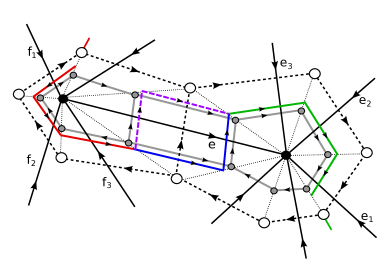
Figure 11: The paths $p_{e,+}=p_{t(e)<}\circ r(\bar{e})\circ r(e)\circ p_{s(e)}^{-1}$ and $p_{e,-}=p_{t(e)<}\circ l(e)\circ l(\bar{e})\circ p_{s(e)}^{-1}$ in ${\Gamma_{D}}$ for an edge $e$ of $\Gamma$ and the subpaths $p_{s(e)<}$ (red), $p_{t(e)<}$ (green), $r(\bar{e})\circ r(e)$ (blue) and $l(e)\circ l(\bar{e})$ (purple).

Lemma 7.2.

Let $\Gamma$ be a regular ciliated ribbon graph and $e$ an edge of $\Gamma$ as in Definition 7.1. Then the holonomies of the paths $p_{e,\pm}$ from (29) coincide and define an algebra homomorphism $\mathrm{Hol}_{p_{e,\pm}}:\mathcal{H}(H)\to\mathcal{H}(H)^{\otimes E}$ given by

$$\mathrm{Hol}_{p_{e,\pm}}=\iota_{e_{1}\ldots e_{i-1}ef_{j-1}\cdots f_{1}}\circ(S^{\tau_{1}}_{D}\otimes...\otimes S^{\tau_{i-1}}_{D}\otimes\mathrm{id}\otimes S^{\rho_{j-1}}_{D}\otimes...\otimes S^{\rho_{1}}_{D})\circ(\phi_{1}^{\otimes(i-1)}\otimes\phi_{1}^{op\otimes(j-1)})\circ\xi_{1}.$$

where $\phi_{1},\xi_{1}:\mathcal{H}(H)\to\mathcal{H}(H)\otimes\mathcal{H}(H)$ are the injective algebra morphisms from Lemma 2.13, $S_{D}$ is the antipode of $D(H)^{*}$ and $2\tau_{k}=1-\epsilon_{k}$, $2\rho_{l}=1-\phi_{l}$.

Proof.

Throughout the proof we denote by $\cdot$ the multiplication of $\mathcal{H}(H)^{\otimes E}$ and by $\cdot^{\prime}$ the multiplication of $D(H)^{*\otimes E}$. From the definition of the holonomy and Lemma 5.3, 5. one obtains

$$\mathrm{Hol}_{p_{e,+}}= \mathrm{Hol}_{p_{t(e)<}}\bullet\mathrm{Hol}_{r(\bar{e})\circ r(e)}\bullet\mathrm{Hol}_{p^{-1}_{s(e)<}}=\mathrm{Hol}_{p_{t(e)<}}\bullet\mathrm{Hol}_{l(e)\circ l(\bar{e})}\bullet\mathrm{Hol}_{p^{-1}_{s(e)<}}=\mathrm{Hol}(p_{e,-}).$$

where $\bullet$ is the multiplication from (16). As $p_{e,+}=p_{t(e)<}\circ r(\bar{e})\circ r(e)\circ p_{s(e)<}^{-1}$ we obtain with Lemma 5.2, Lemma 5.3, 2. and 4. and with the expression for the comultiplication of $D(H)^{*}$ in (2)

$$\mathrm{Hol}_{p_{e},\pm}(y\otimes\gamma) =\Sigma_{i,j}\,\mathrm{Hol}_{p_{t(e)<}}({y}_{({1})}\otimes 1)\cdot^{\prime}({y}_{({2})}\otimes\alpha^{i}\gamma\alpha^{j})_{e}\cdot^{\prime}\mathrm{Hol}_{p_{s(e)<}}(S(x_{j})S({y}_{({3})})x_{i}\otimes 1).$$

As $\Gamma$ has no multiple edges, we have $\{e_{1},...,e_{i-1}\}\cap\{f_{1},...,f_{j-1}\}=\emptyset$. As $e\notin\{e_{1},...,e_{i-1},f_{1},...,f_{j-1}\}$, the three terms in this product commute with respect to $\cdot^{\prime}$ and $\cdot$ and their products with respect to $\cdot^{\prime}$ and to $\cdot$ agree. To compute the holonomies of $p_{t(e)<}$ and $p_{s(e)<}$, we use again Lemma 5.3, 4. together with Lemma 5.2 and the identity $\mathrm{Hol}_{r(\bar{f})^{-1}}=S_{D}\circ\mathrm{Hol}_{r(\bar{f})}$ from Lemma 5.2. This yields

$$\mathrm{Hol}_{p_{t(e)<}}(y\otimes\gamma) =\mathrm{Hol}_{r(\bar{e}_{1}^{\epsilon_{1}})}((y\otimes\gamma)_{(1)})\cdot^{\prime}...\cdot^{\prime}\mathrm{Hol}_{r(\bar{e}_{i-1}^{\epsilon_{i-1}})}((y\otimes\gamma)_{(i-1)})$$

$$=\epsilon(\gamma)\;\mathrm{Hol}_{r(\bar{e}_{1}^{\epsilon_{1}})}({y}_{({1})}\otimes 1)\cdot^{\prime}...\cdot^{\prime}\mathrm{Hol}_{r(\bar{e}_{i-1}^{\epsilon_{i-1}})}({y}_{({i-1})}\otimes 1)$$

$$=\epsilon(\gamma)\;(S^{\tau_{1}}_{D}({y}_{({1})}\otimes 1))_{e_{1}}\cdot^{\prime}...\cdot^{\prime}(S^{\tau_{i-1}}_{D}({y}_{({i-1})}\otimes 1))_{e_{i-1}}$$

and an analogous expression for $p_{s(e)<}$. As all factors in this product commute with respect to $\cdot$ and $\cdot^{\prime}$ and their products with respect to $\cdot^{\prime}$ and $\cdot$ agree, we obtain for the holonomies of the paths $p_{e,\pm}$

$$\mathrm{Hol}_{p_{e},\pm}(y\otimes\gamma)=\Sigma_{i,j}\,\mathrm{Hol}_{p_{t(e)<}}({y}_{({1})}\otimes 1)\cdot({y}_{({2})}\otimes\alpha^{i}\gamma\alpha^{j})_{e}\cdot\mathrm{Hol}_{p_{s(e)<}}(S(x_{i})S({y}_{({3})})x_{j}\otimes 1)$$

with $$\mathrm{Hol}_{p_{t(e)<}}(y\otimes\gamma)=\epsilon(\gamma)\;(S^{\tau_{1}}_{D}({y}_{({1})}\otimes 1))_{e_{1}}\cdot...\cdot(S^{\tau_{i-1}}_{D}({y}_{({i-1})}\otimes 1))_{e_{i-1}}$$

$$\mathrm{Hol}_{p_{s(e)<}}(y\otimes\gamma)=\epsilon(\gamma)\;(S_{D}^{\rho_{1}}({y}_{({1})}\otimes 1))_{f_{1}}\cdot...\cdot(S_{D}^{\rho_{j-1}}({y}_{({j-1})}\otimes 1))_{f_{j-1}}.$$ (30)

Comparing these expressions with the ones for the algebra morphisms $\phi_{1},\xi_{1}:\mathcal{H}(H)\to\mathcal{H}(H)$ from Lemma 2.13 and using that $S_{D}$ is an algebra homomorphism by Lemma 2.13 proves the claim. ∎

With the expressions for the holonomies from Lemma 7.2 we can now prove that they relate the algebra of functions of a $D(H)$-valued Hopf algebra gauge theory on $\Gamma$ to the algebra of triangle operators for the $H$-valued Kitaev model on $\Gamma$.

Theorem 7.3.

Let $\Gamma$ be a regular ciliated ribbon graph. Consider the algebra structure $\mathcal{A}^{*}_{\Gamma}$ from Theorem 4.3 for $K=D(H)$ and the $R$-matrix from (1). For edges $e,f$ of $\Gamma$ set $e<f$ if $e$ and $f$ have no common vertex or if $e$ and $f$ share a vertex $v$ with $e<f$ at $v$. Then the map $\chi:\mathcal{A}^{*}_{\Gamma}\to\mathcal{H}(H)^{op\otimes E}$

$$\chi((y\otimes\gamma)_{e}):=\mathrm{Hol}_{p_{e},\pm}(y\otimes\gamma) \forall e\in E$$

$$\chi((y^{1}\otimes\gamma^{1})_{e_{1}}\cdot_{\mathcal{A}^{*}}...\cdot_{\mathcal{A}^{*}}(y^{k}\otimes\gamma^{k})_{e_{k}}):=\chi((y^{k}\otimes\gamma^{k})_{e_{k}})\cdots\chi((y^{1}\otimes\gamma^{1})_{e_{1}}) \text{if }e_{1}<e_{2}<...<e_{k}.$$

is an algebra homomorphism.

Proof.

Throughout the proof we denote by $\cdot$ the multiplication of $\mathcal{H}(H)^{\otimes E}$, by $\cdot^{\prime}$ the multiplication of $D(H)^{*\otimes E}$ and by $\cdot^{\prime\prime}$ the multiplication of $D(H)^{*}$. As $\Gamma$ is a ribbon graph without loops or multiple edges, we have for any two distinct edges $e,f\in E$ either $e<f$ or $f<e$ or both - the latter if and only if $e$ and $f$ do not share a vertex. As the elements $(y\otimes\gamma)_{e}$ for $e\in E$ generate $\mathcal{A}^{*}_{\Gamma}$ multiplicatively and the elements $(y\otimes\gamma)_{e}$ and $(z\otimes\delta)_{f}$ commute in $\mathcal{A}^{*}_{\Gamma}$ for any two edges $e,f$ that do not share a vertex, the map $\chi$ is well-defined. To show that it is an algebra homomorphism from $\mathcal{A}^{*}_{\Gamma}$ to $\mathcal{H}(H)^{op\otimes E}$, we have to verify the multiplication relations in Proposition 4.4.

As $\Gamma$ has no loops or multiple edges, any two edges $e,f\in E$ satisfies exactly one of the following: (i) $e=f$, (ii) $e$ and $f$ are not incident at a common vertex, (iii) $e$ and $f$ share exactly one vertex. As the paths $p_{e,\pm}$ from Definition 7.1 satisfy the assumptions of Lemma 5.3, 2. and edge reversal in $\mathcal{A}^{*}_{\Gamma}$ corresponds to applying the antipode of $D(H)^{*}$, it is sufficient to consider products of holonomies of the following form:

1. $\mathrm{Hol}_{p_{e},\pm}\cdot\mathrm{Hol}_{p_{e},\pm}$

2. $\mathrm{Hol}_{p_{e},\pm}\cdot\mathrm{Hol}_{p_{f},\pm}$ for edges $e,f$ without a common vertex

3. $\mathrm{Hol}_{p_{e},\pm}\cdot\mathrm{Hol}_{p_{f},\pm}$ with ${\bf t}(e)={\bf t}(f)$, ${\bf s}(e)\neq{\bf s}(f)$ and $e<f$ at ${\bf t}(e)$.

$\bullet$ case (i): In this case, the claim follows directly from the fact that $\mathrm{Hol}_{p_{e},\pm}:\mathcal{H}(H)\to\mathcal{H}(H)^{\otimes E}$ is an algebra morphism by Lemma 7.2.This yields for all $y,z\in H$, $\gamma,\delta\in H^{*}$

$$\mathrm{Hol}_{p_{e,\pm}}(y\otimes\gamma)\cdot\mathrm{Hol}_{p_{e,\pm}}(z\otimes\delta)=\langle{\gamma}_{({1})},{z}_{({2})}\rangle\;\mathrm{Hol}_{p_{e\pm}}(y{z}_{({1})}\otimes{\gamma}_{({2})}\delta).$$

With the expression for the $R$-matrix in (1) and the multiplication of $D(H)^{*}=H^{op}\otimes H$ we obtain

$$\langle(y\otimes\gamma)_{(1)}\otimes(z\otimes\delta)_{(1)},R\rangle\;(y\otimes\gamma)_{(2)}\cdot^{\prime\prime}(z\otimes\delta)_{(2)}=\langle{\gamma}_{({1})},{z}_{({2})}\rangle\;(S({z}_{({3})})y{z}_{({1})}\otimes{\gamma}_{({2})})\cdot^{\prime\prime}({z}_{({4})}\otimes\delta)$$

$$=\langle{\gamma}_{({1})},{z}_{({2})}\rangle\;z_{4}S({z}_{({3})})y{z}_{({1})}\otimes{\gamma}_{({2})}\delta=\langle{\gamma}_{({1})},{z}_{({2})}\rangle\;y{z}_{({1})}\otimes{\gamma}_{({2})}\delta,$$ (31)

which allows us to rewrite the product of the holonomies as

$$\mathrm{Hol}_{p_{e,\pm}}(y\otimes\gamma)\cdot\mathrm{Hol}_{p_{e,\pm}}(z\otimes\delta)=\langle(y\otimes\gamma)_{(1)}\otimes(z\otimes\delta)_{(1)},R\rangle\;\mathrm{Hol}_{p_{e,\pm}}((y\otimes\gamma)_{(2)}\cdot^{\prime\prime}(z\otimes\delta)_{(2)}).$$ (32)

$\bullet$ case (ii): besides the factors $r(\bar{e})$ and $r(e)$, the expression for $p_{e,+}$ involves only factors $r(\bar{g})^{\pm 1}$ (factors $l(\bar{g})^{\pm 1}$) for edges $g\in E$ that are incoming (outgoing) at ${\bf s}(e)$ or ${\bf t}(e)$. It therefore has non-trivial entries only in the copies of $\mathcal{H}(H)$ in $\mathcal{H}(H)^{\otimes E}$ that are associated with $e$ or with such edges $g$. If $g\in E$ is an edge that is incident at one of the vertices ${\bf t}(e)$ and ${\bf s}(e)$ and at one of the vertices ${\bf t}(f)$ and ${\bf s}(f)$, then $g\notin\{e,f\}$ and $g$ contributes a factor $r(\bar{g})^{\pm}$ in one of the paths $p_{e,+}$, $p_{f,+}$ and a factor $l(\bar{g})^{\pm}$ in the other, because it is incoming at one of these vertices and outgoing at the other. By (7) and (19), the holonomies of $r(\bar{g})^{\pm 1}$ and $l(\bar{g})^{\pm 1}$ commute with respect to the multiplication $\cdot^{\prime}$ of $\mathcal{H}(H)^{\otimes E}$. As the different copies of $\mathcal{H}(H)$ in $\mathcal{H}(H)^{\otimes E}$ commute as well, it follows that the holonomies of $p_{e,+}$ and $p_{f,+}$ commute if $e$ and $f$ have no common vertex.

$\bullet$ case (iii): To prove (iii) we decompose the edge paths $p_{e,\pm}$ from (29) as

$$p_{e,+}=p_{t(e)\leq}\circ p_{s(e)<}^{-1} p_{e,-}=p_{t(e)<}\circ p_{s(e)\leq}^{-1}$$ (33)

with $$p_{t(e)\leq}=p_{t(e)<}\circ r(\bar{e})\circ r(e) p_{s(e)\leq}=p_{s(e)<}\circ r(\bar{e}^{-1})\circ r(e^{-1}).$$

Because $\{e_{1},...,e_{i-1}\}\cap\{f_{1},...,f_{j-1}\}=\emptyset$ and $e\notin\{e_{1},...,e_{i-1},f_{1},...,f_{j-1}\}$, the holonomy of $p_{s(e)<}$ commutes with the holonomies of $r(\bar{e})\circ r(e)$, $p_{t(e)<}$ and $p_{t(e)\leq}$, and the holonomy of $p_{t(e)<}$ commutes with the holonomies of $r(\bar{e})\circ r(e)$, $p_{s(e)<}$ and $p_{s(e)\leq}$. As the holonomies of ${r(\bar{e})}$ and ${l(\bar{e})}$ commute due to (7) and (19), the holonomy of $p_{t(e)<}$ (of $p_{s(e)<}$) also commutes with the holonomies of all paths $p_{g,\pm}$, for which $g$ is not not incident at ${\bf t}(e)$ (at ${\bf s}(e)$).

Suppose now that $e,f$ share the vertex ${\bf t}(e)={\bf t}(f)$. As $\Gamma$ has no loops or multiple edges, this implies ${\bf s}(e)\notin\{{\bf s}(f),{\bf t}(e),{\bf t}(f)\}$ and ${\bf s}(f)\notin\{{\bf s}(e),{\bf t}(e),{\bf t}(f)\}$. Due to Lemma 7.2, the fact that $S_{D}:\mathcal{H}(H)\to\mathcal{H}(H)$ and $\phi_{1},\xi_{1}:\mathcal{H}(H)\to\mathcal{H}(H)\otimes\mathcal{H}(H)$ are algebra morphisms by Lemma 2.13 and because $\phi_{1}$ is coassociative, it is sufficient to consider a ciliated ribbon graph $\Gamma$ that consists of a vertex $v$ with two incoming edges $e,f$ such that $e<f$ at $v$ and such that the vertices ${\bf s}(e)$ and ${\bf s}(f)$ are distinct and univalent. In this case one has $p_{e,+}=p_{t(e)\leq}$ and $p_{f,+}=p_{t(f)\leq}$. If one associates the first copy of $\mathcal{H}(H)$ in $\mathcal{H}(H)\otimes\mathcal{H}(H)$ with $e$ and the second with $f$, one obtains

$$\mathrm{Hol}_{p_{e,+}}(y\otimes\gamma)=(y\otimes\gamma)\otimes(1\otimes 1)\qquad\mathrm{Hol}_{p_{f,+}}(y\otimes\gamma)=({y}_{({1})}\otimes 1)\otimes({y}_{({2})}\otimes\gamma),$$

and this implies

$$\mathrm{Hol}_{p_{e,+}}(y\otimes\gamma)\cdot\mathrm{Hol}_{p_{f,+}}(z\otimes\delta)=\langle{\gamma}_{({1})},{z}_{({2})}\rangle\;(y{z}_{({1})}\otimes{\gamma}_{({2})})\otimes({z}_{({3})}\otimes\delta)$$ (34)

$$=\langle{\gamma}_{({1})},{z}_{({2})}\rangle\;(({z}_{({4})}\otimes 1)\cdot(S({z}_{({3})})y{z}_{({1})}\otimes{\gamma}_{({2})}))\otimes({z}_{({5})}\otimes\delta)$$

$$=\langle{\gamma}_{({1})},{z}_{({2})}\rangle\;\mathrm{Hol}_{p_{e,+}}({z}_{({4})}\otimes\delta)\cdot\mathrm{Hol}_{p_{f,+}}(S({z}_{({3})})y{z}_{({1})}\otimes{\gamma}_{({2})}).\qquad\qquad\qquad\qquad$$

With formula (7) this yields

$$\mathrm{Hol}_{p_{e,+}}(y\otimes\gamma)\!\cdot\!\mathrm{Hol}_{p_{f,+}}(z\otimes\delta)\!=\!\langle(y\otimes\gamma)_{(1)}\!\otimes\!(z\otimes\delta)_{(1)},R\rangle\;\mathrm{Hol}_{p_{f,+}}((z\otimes\delta)_{(2)})\!\cdot\!\mathrm{Hol}_{p_{e,+}}((y\otimes\gamma)_{(2)}).$$

Comparing this expression and expression (32) with the multiplication relations in Proposition 4.4 then proves that $\chi:\mathcal{A}^{*}_{\Gamma}\to\mathcal{H}(H)^{op\otimes E}$ is an algebra homomorphism. ∎

We will now show that the linear map $\chi:\mathcal{A}^{*}_{\Gamma}\to\mathcal{H}(H)^{\otimes E}$ is not only an algebra homomorphism but an algebra isomorphism. This is achieved by expressing it in terms of certain algebra homomorphisms from the algebra of functions $\mathcal{A}^{*}_{v}$ on each vertex neighbourhood $\Gamma_{v}$ into $\otimes_{v\in V}\mathcal{H}(H)^{\otimes|v|}$. These algebra homomorphisms are obtained from the holonomies of paths in ${\Gamma_{D}}$ that generalise the paths $p_{e,\pm}$ from Definition 7.1.

Definition 7.4.

Let $v$ be a ciliated vertex with $n$ incident edges $e_{1},...e_{n}$, numbered according to the ordering at $v$ and such that $e_{1}^{\epsilon_{1}}$,…, $e_{n}^{\epsilon_{n}}$ are incoming. Then for $i\in\{1,...,n\}$ we define

$$p_{e_{i},0}:=r(\bar{e}_{1}^{\epsilon_{1}})\circ...\circ r(\bar{e}_{i-1}^{\epsilon_{i-1}})\circ r(\bar{e}_{i})\circ r(e_{i})\qquad p_{e_{i},1}:=r(\bar{e}_{1}^{\epsilon_{1}})\circ...\circ r(\bar{e}_{i-1}^{\epsilon_{i-1}})\circ l(e_{i}).$$

We equip the vector space $(H\otimes H^{*})^{\otimes n}$ with the algebra structure $\mathcal{A}^{*}_{v}$ from Definition 4.2 for the Hopf algebra $K=D(H)$, arbitrary parameters $\sigma_{i}\in\{0,1\}$ and the universal $R$-matrix from (1).

Lemma 7.5.

The map $\chi_{\tau,\sigma}:\mathcal{A}^{*}_{v}\to\mathcal{H}(H)^{op\otimes n}$ with

$$\chi_{\tau,\sigma}((y\otimes\gamma)_{i})=\mathrm{Hol}_{p_{e_{i}},\sigma_{i}}(y\otimes\gamma)$$

$$\chi_{\tau,\sigma}(y^{1}\otimes\gamma^{1}\otimes...\otimes y^{n}\otimes\gamma^{n})=\chi_{\tau,\sigma}((y^{n}\otimes\gamma^{n})_{n})\cdot...\cdot\chi_{\tau,\sigma}((y^{1}\otimes\gamma^{1})_{1})$$

is an algebra homomorphism. It is an isomorphism iff $\sigma_{i}=0$ for all $i\in\{1,...,n\}$ or $\dim_{\mathbb{F}}(H)=1$.

Proof.

If we identify the $i$th copy of $\mathcal{H}(H)$ in $\mathcal{H}(H)^{\otimes n}$ with the $i$th edge $e_{i}$, then by the proof of Lemma 7.2 the holonomies of the paths $p_{e_{i},\sigma_{i}}$ are given by

$$\mathrm{Hol}_{p_{e_{i},\sigma_{i}}}=(S^{\tau_{1}}_{D}\otimes...\otimes S^{\tau_{n}}_{D})\circ\mathrm{Hol}_{p_{e_{i},\sigma}}^{\tau=0}\circ S^{\tau_{i}}_{D},$$

where $$\mathrm{Hol}_{p_{e_{i},\sigma_{i}}}^{\tau=0}(y\otimes\gamma)=\begin{cases}({y}_{({1})}\otimes 1)\otimes...\otimes({y}_{({i-1})}\otimes 1)\otimes({y}_{({i})}\otimes\gamma)\otimes(1\otimes 1)^{\otimes(n-i)}&\sigma_{i}=0\\ ({y}_{({1})}\otimes 1)\otimes...\otimes({y}_{({i-1})}\otimes 1)\otimes S_{D}(1\otimes S(\gamma))\otimes(1\otimes 1)^{\otimes(n-i)}&\sigma_{i}=1\end{cases}$$

denotes the holonomies for the case where all edges $e_{1},...,e_{n}$ are incoming at $v$, $2\tau_{i}=1-\epsilon_{i}$ and $S_{D}$ is the antipode of $D(H)^{*}$. The map $S_{D}:\mathcal{H}(H)\to\mathcal{H}(H)$ is an algebra isomorphism by Lemma 2.13, and the algebra structure from Definition 4.2 for general edge orientation is defined by the condition that $S^{\tau_{1}}_{D}\otimes...\otimes S^{\tau_{n}}_{D}$ is an algebra morphism to the corresponding algebra structure for $\tau_{1}=...=\tau_{n}=0$. It is therefore sufficient to consider the case $\tau_{i}=0$ for all $i\in\{1,...,n\}$. If $\sigma_{i}=0$ for all $i\in\{1,....,n\}$ the claim follows from Theorem 7.3, applied to a graph that consists of a central vertex $v$ with $n$ incident edges and $n$ univalent vertices. For general $\sigma$, we have

$$(\chi_{0,\sigma}\circ\iota_{i})(y\otimes\gamma)=\begin{cases}\phi_{1}^{(i-1)}(y\otimes\gamma)\otimes(1\otimes 1)^{\otimes(n-i)}&\sigma_{i}=0\\ \phi_{1}^{(i-2)}(y\otimes 1)\otimes S_{D}(1\otimes S(\gamma))\otimes(1\otimes 1)^{\otimes(n-i)}&\sigma_{i}=1,\end{cases}$$

where $\phi_{1}:\mathcal{H}(H)\to\mathcal{H}(H)\otimes\mathcal{H}(H)$ is the coassociative algebra homomorphism from Lemma 2.13. It is therefore sufficient to consider the case $n=2$ and to compute the products $(y\otimes\gamma)_{i}\cdot(y\otimes\gamma)_{i}$ for $i\in\{1,2\}$ and $\sigma_{i}=1$, $(y\otimes\gamma)_{1}\cdot(z\otimes\delta)_{2}$ for $\sigma_{1}=\sigma_{2}=1$, $\sigma_{1}=1-\sigma_{2}=0$ and $\sigma_{1}=1-\sigma_{2}=1$. For the first two cases, we obtain

$$\chi_{0,\sigma}((y\otimes\gamma)_{1})\cdot\chi_{0,\sigma}((z\otimes\delta)_{1})=\epsilon(y)\epsilon(z)\big{(}S_{D}(1\otimes S(\gamma))\otimes(1\otimes 1)\big{)}\cdot\big{(}S_{D}(1\otimes S(\delta))\otimes(1\otimes 1)\big{)}$$

$$=\epsilon(yz)\,S_{D}(1\otimes S(\delta\gamma))\otimes(1\otimes 1)=\chi_{0,\sigma}((yz\otimes\delta\gamma)_{1})=\chi_{0,\sigma}((z\otimes\delta)\cdot^{\prime\prime}(y\otimes\gamma))$$

$$\chi_{0,\sigma}((y\otimes\gamma)_{2})\cdot\chi_{0,\sigma}((z\otimes\delta)_{2})=\big{(}({y}_{({1})}\otimes 1)\otimes(S_{D}(1\otimes S(\gamma)))\big{)}\cdot\big{(}({z}_{({1})}\otimes 1)\otimes(S_{D}(1\otimes S(\delta)))\big{)}\quad$$

$$=({y}_{({1})}{z}_{({1})}\otimes 1)\otimes(S_{D}(1\otimes S({\delta}_{({\gamma})})))=\chi_{0,\sigma}(yz\otimes\delta\gamma)=\chi_{0,\sigma}((z\otimes\delta)\cdot^{\prime\prime}(y\otimes\gamma)),$$

where $\cdot^{\prime\prime}$ denotes the multiplication of $D(H)^{*}=H^{op}\otimes H^{*}$. If $\sigma_{1}=1-\sigma_{2}=0$, we obtain

$$\chi_{0,\sigma}((y\otimes\gamma)_{1})\cdot\chi_{0,\sigma}((z\otimes\delta)_{2})=\big{(}(y\otimes\gamma)\otimes(1\otimes 1)\big{)}\cdot\big{(}({z}_{({1})}\otimes 1)\otimes S_{D}(1\otimes S(\delta))\big{)}$$

$$=\langle{\gamma}_{({1})},{z}_{({2})}\rangle\,(y{z}_{({1})}\otimes{\gamma}_{({2})})\otimes S_{D}(1\otimes S(\delta))$$

$$=\langle{\gamma}_{({1})},{z}_{({2})}\rangle\,\big{(}({z}_{({4})}\otimes 1)\otimes S_{D}(1\otimes S(\delta))\big{)}\cdot\big{(}(S({z}_{({3})})yz_{1}\otimes\gamma)\otimes(1\otimes 1)\big{)}$$

$$=\langle(y\otimes\gamma)_{(1)}\otimes(z\otimes\delta)_{(1)},R\rangle\,\chi_{0,\sigma}(((z\otimes\delta)_{(2)})_{2})\cdot\chi_{0,\sigma}(((y\otimes\gamma)_{(2)})_{1}),\qquad\qquad\qquad\qquad\qquad$$

where we used equation (7) in the last step. Similarly, for $\sigma_{1}=1-\sigma_{2}=1$ we have

$$\chi_{0,\sigma}((y\otimes\gamma)_{1})\cdot\chi_{0,\sigma}((z\otimes\delta)_{2})=\epsilon(y)\,\big{(}S_{D}(1\otimes S(\gamma))\otimes(1\otimes 1)\big{)}\cdot\big{(}({z}_{({1})}\otimes 1)\otimes({z}_{({2})}\otimes\delta)\big{)}$$

$$=\epsilon(y)\,\big{(}(x_{k}S(x_{l})\otimes\alpha^{l}\gamma\alpha^{k})\otimes(1\otimes 1)\big{)}\cdot\big{(}({z}_{({1})}\otimes 1)\otimes({z}_{({2})}\otimes\delta)\big{)}$$

$$=\epsilon(y)\langle\alpha^{l}_{(1)}{\gamma}_{({1})}\alpha^{k}_{(1)},{z}_{({2})}\rangle\,(x_{k}S(x_{l}){z}_{({1})}\otimes\alpha^{l}_{(2)}{\gamma}_{({2})}\alpha^{k}_{(2)})\otimes({z}_{({3})}\otimes\delta)$$

$$=\epsilon(y)\langle{\gamma}_{({1})},{z}_{({1})}\rangle\,({z}_{({2})}x_{k}S(x_{l})\otimes\alpha^{l}{\gamma}_{({2})}\alpha^{k})\otimes({z}_{({3})}\otimes\delta)$$

$$=\epsilon(S({z}_{({3})})y{z}_{({1})})\langle{\gamma}_{({1})},{z}_{({2})}\rangle\,\big{(}({z}_{({4})}\otimes 1)\otimes({z}_{({5})}\otimes\delta)\big{)}\cdot\big{(}(x_{k}S(x_{l})\otimes\alpha^{l}{\gamma}_{({2})}\alpha^{k})\otimes(1\otimes 1)\big{)}$$

$$=\langle(y\otimes\gamma)_{(1)}\otimes(z\otimes\delta)_{(1)},R\rangle\,\chi_{0,\sigma}(((z\otimes\delta)_{(2)})_{2})\cdot\chi_{0,\sigma}(((y\otimes\gamma)_{(2)})_{1}),\qquad\;\;\;$$

and an analogous computation yields the same identity for $\sigma_{1}=\sigma_{2}=1$. Comparing these expressions with the multiplication relations in Theorem 4.1 proves that $\chi_{0,\sigma}$ is an algebra homomorphism. Clearly, $\chi_{\tau,\sigma}$ is bijective if $\dim_{\mathbb{F}}(H)=1$. To show that for $\dim_{\mathbb{F}}(H)>1$ the map $\chi_{\tau,\sigma}$ is bijective if and only if $\sigma_{i}=0$ for all $i\in\{1,...,n\}$, it is again sufficient to consider the case $\tau_{1}=...=\tau_{n}=0$, because the map $S^{\tau_{1}}_{D}\otimes...\otimes S^{\tau_{n}}_{D}$ is an involution. For $\sigma_{1}=...=\sigma_{n}=0$ one has

$$\chi_{0,0}((y^{1}\otimes\gamma^{1})\otimes...\otimes(y^{n}\otimes\gamma^{n}))$$

$$=(y^{n}_{(1)}\cdots y^{2}_{(1)}y^{1}\otimes\gamma^{1})\otimes(y^{n}_{(2)}\cdots y^{2}_{(2)}\otimes\gamma^{2})\otimes\ldots\otimes(y^{n}_{(n-1)}y^{n-1}_{(n-1)}\otimes\gamma^{n-1})\otimes(y^{n}_{(n)}\otimes\gamma^{n}),$$

and hence $\chi_{0,0}$ is invertible with inverse

$$\chi_{0,0}^{-1}((z^{1}\otimes\delta^{1})\otimes...\otimes(z^{n}\otimes\delta^{n}))$$

$$=(S(z^{2}_{(1)})z^{1}\otimes\delta^{1})\otimes(S(z^{3}_{(1)})z^{2}_{(2)}\otimes\delta^{2})\otimes...\otimes(S(z^{n}_{(1)})z^{n-1}_{(2)}\otimes\delta^{n-1})\otimes(z^{n}_{(2)}\otimes\delta^{n}).\qquad$$

If $k=\mathrm{min}\{i:\sigma_{i}=1\}\in\{1,...,n\}$ and $\dim_{\mathbb{F}}(H)>1$, one has

$$\chi_{0,\sigma}((S({y}_{({1})})\otimes 1)_{k-1}\cdot_{\mathcal{A}^{*}}({y}_{({2})}\otimes 1)_{k})=\phi_{1}^{(k-2)}({y}_{({2})}S({y}_{({1})})\otimes 1)\otimes(1\otimes 1)^{\otimes(n-k+1)}=\epsilon(y)\,(1\otimes 1)^{\otimes n}.$$

As $\dim_{\mathbb{F}}(H)>1$ implies $\mathrm{ker}(\epsilon)\neq\{0\}$, it follows that $\mathrm{ker}(\chi_{0,\sigma})\neq\{0\}$. ∎

The paths $p_{e_{i},\sigma_{i}}$ in the vertex neighbourhoods that define the algebra homomorphism $\chi_{\sigma,\tau}$ give a geometrical interpretation to the parameters $\sigma_{i}\in\{0,1\}$ that arise in the definition of a Hopf algebra gauge theory in Theorem 4.1. While it was shown in [38] that these parameters are necessary to combine the algebra structures on the different vertex neighbourhoods into an algebra, i. e. to ensure that the image of the map $G^{*}$ from (15) is a subalgebra of $\otimes_{v\in V}\mathcal{A}^{*}_{v}$, they were introduced there by purely algebraic considerations. From the perspective of the Kitaev model they have a geometrical meaning. Passing from the ciliated ribbon graph $\Gamma$ to its vertex neighbourhoods $\Gamma_{v}$ involves a subdivision of each edge $e$ of $\Gamma$ into two edge ends $s(e)$ and $t(e)$. The paths $p_{e,\pm}$ from Definition 7.1 then correspond to the paths

$$p^{\prime}_{e,+}=p_{t(e)<}\circ r(\overline{t(e)})\circ r(t(e))\circ r(s(e))\circ p^{-1}_{s(e)<}=p_{t(e),0}\circ p_{s(e),1}^{-1}$$

$$p^{\prime}_{e,-}=p_{t(e)<}\circ l(t(e))\circ l(s(e))\circ l(\overline{s(e)})\circ p^{-1}_{s(e)<})=p_{t(e),1}\circ p_{s(e),0}^{-1}$$

in the thickening of the subdivided graph, which split naturally into paths $p_{t(e),\sigma}$ and $p_{s(e),1-\sigma}$ in the vertex neighbourhoods $\Gamma_{{\bf t}(e)}$ and $\Gamma_{{\bf s}(e)}$, as shown in Figure 12. These are precisely the paths from Definition 7.4 whose holonomies define the algebra homomorphism in Lemma 7.5. Hence, the parameters $\sigma_{i}\in\{0,1\}$ in Theorem 4.1 describe the splitting of the associated paths $p^{\prime}_{e,\pm}$ in the thickened graph into two paths $p_{t(e),\sigma}$ and $p_{s(e),1-\sigma}$ in the vertex neighbourhoods $\Gamma_{{\bf t}(e)}$ and $\Gamma_{{\bf s}(e)}$.

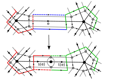
Figure 12: The paths $p_{e,\pm}$ in ${\Gamma_{D}}$ and the splitting of the associated paths $p^{\prime}_{e,\pm}$ in the thickening of the subdivision into paths $p_{t(e),0}$, $p_{t(e),1}$ (green) and $p_{s(e),0}$, $p_{s(e),1}$ (red) in the vertex neighbourhoods of $t(e)$ and $s(e)$.

Theorem 7.6.

For any regular ciliated ribbon graph $\Gamma$, the map $\chi:\mathcal{A}^{*}_{\Gamma}\to\mathcal{H}(H)^{op\otimes E}$ from Theorem 7.3 is an algebra isomorphism.

Proof.

As $\mathcal{A}^{*}_{\Gamma}\cong(H\otimes H^{*})^{\otimes E}\cong\mathcal{H}(H)^{\otimes E}$ as vector spaces, it is sufficient to show that $\chi$ is injective. We relate $\chi$ to the maps from Lemma 7.5 via the injective linear map $G^{*}:\mathcal{A}^{*}_{\Gamma}\to\otimes_{v\in V}\mathcal{A}^{*}_{v}$ from (15). For this, define ${\boldsymbol{\rho}}:E(\Gamma)\to\cup_{v\in V}E(\Gamma_{v})$ by setting ${\boldsymbol{\rho}}(e)=t(e)$ for each edge $e\in E(\Gamma)$. For each vertex neighbourhood $\Gamma_{v}$ and edge end $f\in E(\Gamma_{v})$ we set $\tau_{f}=\sigma_{f}=0$ if $f$ is incoming at $v$ and $\tau_{f}=\sigma_{f}=1$ else and equip $\Gamma_{v}$ with the algebra structure $\mathcal{A}^{*}_{v}$ from Definition 4.2. Then by Theorem 4.3 the algebra $\mathcal{A}^{*}_{\Gamma}$ is isomorphic to the image of $G^{*}$. Denote by $\chi_{v}=\chi_{\tau_{v},\sigma_{v}}:\mathcal{A}^{*}_{v}\to\mathcal{H}(H)^{\otimes|v|}$ the linear map from Lemma 7.5 for the vertex neighbourhood $\Gamma_{v}$. Then one has

$$\chi=M^{*}\circ(\otimes_{v\in V}\chi_{v})\circ G^{*}\quad\text{with}$$

$$M^{*}:\otimes_{v\in V}\mathcal{H}(H)^{\otimes|v|}\to\mathcal{H}(H)^{\otimes E},\quad(y\otimes\gamma\otimes z\otimes\delta)_{t(e)s(e)}\mapsto\epsilon(\delta)\,(yz\otimes\gamma)_{e}.$$

From the definition of $\chi_{v}=\chi_{\sigma_{v}\tau_{v}}$ in Lemma 7.5 it follows that the restriction of $M^{*}$ to the image of $(\otimes_{v\in V}\chi_{v})\circ G^{*}_{e}$ is injective. Hence, it is sufficient to prove that $(\otimes_{v\in V}\chi_{v})\circ G^{*}:\mathcal{A}^{*}_{\Gamma}\to\otimes_{v\in V}\mathcal{H}(H)^{\otimes|v|}$ is injective. For this we assign to a vertex $v$ of $\Gamma$ of valence $|v|=n$ the map

$$\mu_{v}=(S_{D}^{\tau_{1}}\otimes...\otimes S_{D}^{\tau_{n}})\circ\mu_{v,0}\circ(S_{D}^{\tau_{1}}\otimes...\otimes S_{D}^{\tau_{n}}):\mathcal{H}(H)^{\otimes n}\to\mathcal{A}^{*}_{v}$$

$$\mu_{v,0}(z^{1}\otimes\delta^{1}\otimes...\otimes z^{n}\otimes\delta^{n})=(S(z^{2}_{(1)})z^{1}\otimes\delta^{1})\otimes(S(z^{3}_{(1)})z^{2}_{(2)}\otimes\delta^{2})\otimes....\otimes(z^{n}_{(2)}\otimes\delta^{n}),$$

as in the proof of Lemma 7.5. Then $\mu_{v}\circ\chi_{v}=(S_{D}^{\tau_{1}}\otimes...\otimes S_{D}^{\tau_{n}})\circ\mu_{v,0}\circ\chi_{v,0}\circ(S_{D}^{\tau_{1}}\otimes...\otimes S_{D}^{\tau_{n}})$ and

$$\mu_{v,0}\circ\chi_{v,0}(y^{1}\otimes\gamma^{1}\otimes...\otimes y^{n}\otimes\gamma^{n})$$

$$=m_{1}(y^{1}\otimes y^{2}_{(1)}\otimes\gamma^{1})\otimes m_{2}(y^{2}_{(2)}\otimes y^{3}_{(1)}\otimes\gamma^{2})\otimes...\otimes m_{n-1}(y^{n-1}_{(2)}\otimes y^{n}_{(1)}\otimes\gamma^{n-1})\otimes m_{n}(y^{n}_{(2)}\otimes 1\otimes\gamma^{n})$$

$$\text{with}\quad m_{i}(y\otimes z\otimes\delta)=\begin{cases}\epsilon(z)\,y\otimes\delta&\sigma_{i}=\sigma_{i+1}=0\\ \epsilon(y)\,\Sigma_{r,s}\,zx_{r}S(x_{s})\otimes\alpha^{s}\delta\alpha^{r}&\sigma_{i}=\sigma_{i+1}=1\\ \epsilon(y)\epsilon(z)\Sigma_{r,s}\,x_{r}S(x_{s})\otimes\alpha^{s}\delta\alpha^{r}&\sigma_{i}=1-\sigma_{i+1}=1\\ zy\otimes\delta&\sigma_{i}=1-\sigma_{i+1}=0,\end{cases}$$

where we set $\sigma_{n+1}=0$. As $(\epsilon\otimes\mathrm{id})\circ\Delta=(\mathrm{id}\otimes\epsilon)\circ\Delta=\mathrm{id}$ and for each edge $e$ of $\Gamma$ one has $\sigma_{s(e)}=1-\sigma_{t(e)}=0$, it follows that $(\otimes_{v\in V}\mu_{v})\circ(\otimes_{v\in V}\chi_{v})\circ G^{*}:\mathcal{A}^{*}_{\Gamma}\to\otimes_{v\in V}\mathcal{H}(H)^{\otimes|v|}$ is injective unless there is a finite sequence of edges $e_{1}$, $e_{2}$,…., $e_{n}$ such that ${\bf t}(e_{i})={\bf s}(e_{i+1})$ for $i\in\{1,...,n-1\}$, ${\bf t}(e_{n})={\bf s}(e_{1})$, $e_{i}$ and $e_{i+1}$ are adjacent at ${\bf s}(e_{i+1})={\bf t}(e_{i})$ with $e_{i+1}<e_{i}$ and $e_{1}$ and $e_{n}$ are adjacent at ${\bf s}(e_{1})={\bf t}(e_{n})$ with $e_{1}<e_{n}$. However, this implies that the path $f=e_{1}^{-1}\circ...\circ e_{n}^{-1}$ is a ciliated face that represents a face of $\Gamma$ that does not contain a cilium, a contradiction to the assumption that $\Gamma$ is regular. Hence $(\otimes_{v\in V}\mu_{v})\circ(\otimes_{v\in V}\chi_{v})\circ G^{*}:\mathcal{A}^{*}_{\Gamma}\to\otimes_{v\in V}\mathcal{H}(H)^{\otimes|v|}$ and $(\otimes_{v\in V}\chi_{v})\circ G^{*}$ are injective, and the claim follows. ∎

8 The quantum moduli algebra and the protected space

The last section proves that for each regular ciliated ribbon graph $\Gamma$, the algebra $\mathcal{H}(H)^{op\otimes E}$ of triangle operators for a $H$-valued Kitaev model on $\Gamma$ is isomorphic to the algebra of functions $\mathcal{A}^{*}_{\Gamma}$ of a $D(H)$-valued Hopf algebra gauge theory. In this section we show, that the isomorphism $\chi:\mathcal{A}^{*}_{\Gamma}\to\mathcal{H}(H)^{op\otimes E}$ is compatible with the action of gauge symmetries and the curvatures in the two models. We start by proving that it is a module morphism with respect to the $D(H)^{\otimes V}$-module structures on $\mathcal{A}^{*}_{\Gamma}$ and on $\mathcal{H}(H)^{op\otimes E}$. We then show that it sends the holonomies of faces of $\Gamma$ that are based at the cilium of $\Gamma$ to the product of the associated vertex and face operator. The final result is an algebra isomorphism between the quantum moduli algebra of the Hopf algebra gauge theory from Theorem 4.9 and the subalgebra of Kitaev’s triangle operator algebra from Lemma 6.3.

To show that the map $\chi:\mathcal{A}^{*}_{\Gamma}\to\mathcal{H}(H)^{op\otimes E}$ from Theorem 7.3 is not only an algebra isomorphism but also a module morphism with respect to gauge transformations, we consider the $D(H)^{\otimes V}$-right module algebra structure on the algebra $\mathcal{A}^{*}_{\Gamma}$ from Theorem 4.3 and Proposition 4.4 and the $D(H)^{\otimes V}$-right module algebra structure on the algebra $\mathcal{H}(H)^{op\otimes E}$ from Theorem 6.1.

Theorem 8.1.

Let $\Gamma$ be a regular ciliated ribbon graph. Then for all edges $e$ of $\Gamma$ one has

$$\mathrm{Hol}_{p_{e,\pm}}(y\otimes\gamma)\lhd(\delta\otimes z)_{v} =\begin{cases}\epsilon(z)\epsilon(\delta)\,\mathrm{Hol}_{p_{e,\pm}}(y\otimes\gamma)&v\notin\{{\bf s}(e),{\bf t}(e)\}\\ \langle\delta\otimes z,(y\otimes\gamma)_{(1)}\rangle\;\mathrm{Hol}_{p_{e,\pm}}((y\otimes\gamma)_{(2)})&v={\bf t}(e)\\ \langle\delta\otimes z,S_{D}((y\otimes\gamma)_{(2)})\rangle\;\mathrm{Hol}_{p_{e,\pm}}((y\otimes\gamma)_{(1)})&v={\bf s}(e).\end{cases}$$

The map $\chi:\mathcal{A}^{*}_{\Gamma}\to\mathcal{H}(H)^{op\otimes E}$ from Theorem 7.3 is an isomorphism of $D(H)^{\otimes V}$-right module algebras and restricts to an algebra isomorphism $\chi:\mathcal{A}^{*}_{\Gamma\,inv}\to\mathcal{H}(H)^{op\otimes E}_{inv}$.

Proof.

1. Denote for each vertex $v$ by $f(v)$ the ciliated face of $\Gamma$ that starts and ends at the cilium at $v$ and by $p_{v}$ and $p_{f(v)}$ the associated vertex and face loop in ${\Gamma_{D}}$. To prove the first equation in the theorem, we consider a vertex $v\notin\{{\bf s}(e),{\bf t}(e)\}$ and show that the holonomies of $p_{v}$ and $p_{f(v)}$ commute with the holonomy of $p_{e,\pm}$. The equation then follows from the formula for the $D(H)^{\otimes V}$-module structure in Theorem 6.1. For this, note that the vertex loop $p_{v}$ is composed of paths $r(\bar{g})$ and $l(\bar{g})^{-1}$ for edges $g\in E(\Gamma)$ incident at $v$. The path $p_{e,\pm}$ is composed of paths $r(\bar{h})^{\pm 1}$, $l(\bar{h})^{\pm 1}$, $r(h)^{\pm 1}$, $l(h)^{\pm 1}$ for $h\in E(\Gamma)$ incident at ${\bf s}(e)$ or ${\bf t}(e)$. It follows that the holonomy of $p_{v}$ commutes with the holonomy of $p_{e,\pm}$ if $v\notin\{{\bf s}(e),{\bf t}(e)\}$.

To prove the corresponding statement for the face loop $p_{f(v)}$, consider an edge $e$ as in Definition 7.1 and let $p_{e,\pm}$ be the associated edge path from (29). As $S_{D}:\mathcal{H}(H)\to\mathcal{H}(H)$ is an algebra morphism, we can suppose that all edges $e_{1}$,…,$e_{i-1}$ and $f_{1}$,…,$f_{j-1}$ are incoming. If $v\notin\{{\bf s}(e),{\bf t}(e)\}$ the regularity of $\Gamma$ implies that $f(v)$ does no traverse the cilium at ${\bf s}(e)$ or ${\bf t}(e)$ and the edges $e_{1},...,e_{i-1},f_{1},...,f_{j-1},e$ and their inverses are not the first or last edge in $f(v)$. Hence, the face loop $p_{f(v)}$ can be decomposed into

1. subpaths which do not contain $r(g)^{\pm 1}$ or $l(g)^{\pm 1}$ for $g\in\{e_{1},...,e_{i-1},e,f_{1},..,f_{j-1}\}$,

2. subpaths of the form $l(e_{a+1})^{-1}\circ r(e_{a})$ or $l(f_{b+1})^{-1}\circ r(f_{b})$ with $1\leq a\leq i-1$, $1\leq b\leq j-1$,

3. subpaths of the form $r(e)\circ r(f_{j-1})$ or $l(e)^{-1}\circ r(e_{i-1})$,

as shown in Figure 10. The holonomies of the paths in (i) commute with the holonomy of $p_{e,\pm}$ by definition of $\mathcal{H}(H)^{\otimes E}$, the holonomies of the paths in (ii) and the holonomy of $l(e)^{-1}\circ r(e_{i-1})$ in (iii) commute with the holonomy of $p_{e,\pm}$ by Lemma 5.8. The same holds for the holonomy of $r(e)\circ r(f_{j-1})$ in (iii), since $r(e)\circ r(f_{j-1})=l(e)^{-1}\circ r(f_{j-1})$ and $\mathrm{Hol}_{p_{e,\pm}^{-1}}=\mathrm{Hol}_{p_{e^{-1},\pm}}$ by Lemma 7.2. This shows that the holonomy of $p_{f(v)}$ commutes with the holonomies of all paths $p_{e,\pm}$ with $v\notin\{{\bf s}(e),{\bf t}(e)\}$ and completes the proof of the first equation.

2. As $\mathrm{Hol}_{p_{e^{-1},\pm}}=\mathrm{Hol}_{p_{e,\pm}^{-1}}=\mathrm{Hol}_{p_{e,\pm}}\circ S_{D}$ and $\Delta\circ S_{D}=(S_{D}\otimes S_{D})\circ\Delta^{op}$ in $D(H)^{*}$, the third equation follows from the second equation. To prove the second equation, we compute the commutation relations of the holonomies of $p_{v}$ and $p_{f(v)}$ with the holonomy of $p_{e,\pm}$ for $v={\bf t}(e)$. Due to the formula in Lemma 7.2 and because $S_{D}:\mathcal{H}(H)\to\mathcal{H}(H)$ is an algebra morphism by Lemma 2.13, it is sufficient to consider a vertex $v$ at which all edges are incoming. Suppose that the incident edges at $v$ are $e_{1},...,e_{n}$, numbered according to the ordering at $v$.

2(a). We start by computing the commutation relations of the holonomy of the vertex loop $p_{v}$ with the holonomies of the paths $p_{e_{i},\pm}$. As the edges $e_{1},..,e_{n}$ are incoming at $v$, one has $p_{v}=r(\bar{e}_{1})\circ\ldots\circ r(\bar{e}_{n})$, and the paths $p_{e_{i},+}$ can be decomposed as $p_{e_{i},+}=p_{t(e_{i})\leq}\circ p_{s(e_{i})<}^{-1}$, where $p_{t(e_{i})\leq}=p_{t(e_{i})<}\circ r(\bar{e_{i}})\circ r(e_{i})$. Note that $p_{s(e_{i})<}$ does not contain the factors $r(\bar{e}_{i})$, $l(\bar{e}_{i})$, $r(e_{i})$ and $l(e_{i})$ or their inverses since $\Gamma$ has no loops or multiple edges. It follows that the holonomy of $p_{v}$ commutes with the holonomy of $p_{s(e_{i})<}$ for all $i\in\{1,...,n\}$. As $\mathrm{Hol}_{p_{v}}(z\otimes\delta)=\epsilon(\delta)\,\mathrm{Hol}_{p_{t(e_{n})\leq}}(z\otimes 1)$, equation (34) implies for the paths $p_{t(e_{i})\leq}$ with $i\in\{1,...,n-1\}$

$$\mathrm{Hol}_{p_{t(e_{i})\leq}}(y\otimes\gamma)\cdot\mathrm{Hol}_{p_{v}}(z\otimes 1)=\langle{\gamma}_{({1})},{z}_{({2})}\rangle\;\mathrm{Hol}_{p_{v}}({z}_{({4})}\otimes 1)\cdot\mathrm{Hol}_{p_{t(e_{i})\leq}}(S({z}_{({3})})y{z}_{({1})}\otimes\gamma).\qquad\qquad$$

For the paths $p_{e_{n},\pm}$ we obtain the same identity using the fact that $\mathrm{Hol}_{p_{e_{n},\pm}}:\mathcal{H}(H)\to\mathcal{H}(H)^{\otimes E}$ is an algebra morphism by Lemma 2.13:

$$\mathrm{Hol}_{p_{t(e_{n})\leq}}(y\otimes\gamma)\cdot\mathrm{Hol}_{p_{v}}(z\otimes 1)=\mathrm{Hol}_{p_{t(e_{n})\leq}}(y\otimes\gamma)\cdot\mathrm{Hol}_{p_{t(e_{n})\leq}}(z\otimes 1)$$

$$=\langle{\gamma}_{({1})},{z}_{({2})}\rangle\;\mathrm{Hol}_{p_{t(e_{n})\leq}}({z}_{({1})}y\otimes{\gamma}_{({2})})=\langle{\gamma}_{({1})},{z}_{({2})}\rangle\;\mathrm{Hol}_{p_{t(e_{n})\leq}}({z}_{({4})}S({z}_{({3})})y{z}_{({1})}y\otimes{\gamma}_{({2})})\qquad\qquad\quad\;$$

$$=\langle{\gamma}_{({1})},{z}_{({2})}\rangle\;\mathrm{Hol}_{p_{t(e_{n})\leq}}({z}_{({4})}\otimes 1)\cdot\mathrm{Hol}_{p_{t(e_{n})\leq}}(S({z}_{({3})})y{z}_{({1})}\otimes\gamma)$$

$$=\langle{\gamma}_{({1})},{z}_{({2})}\rangle\;\mathrm{Hol}_{p_{v}}({z}_{({4})}\otimes 1)\cdot\mathrm{Hol}_{p_{t(e_{n})\leq}}(S({z}_{({3})})y{z}_{({1})}\otimes\gamma).$$

This implies for all $i\in\{1,...,n\}$

$$\mathrm{Hol}_{p_{e_{i},\pm}}(y\otimes\gamma)\lhd(1\otimes z)_{v}$$ (35)

$$=\mathrm{Hol}_{p_{v}}(S({z}_{({2})})\otimes 1)\cdot\mathrm{Hol}_{p_{t(e_{i})\leq}}((y\otimes\gamma)_{(1)})\cdot\mathrm{Hol}_{p_{s(e_{i})<}^{-1}}((y\otimes\gamma)_{(2)})\cdot\mathrm{Hol}_{p_{v}}({z}_{({1})}\otimes 1)$$

$$=\Sigma_{k,l}\,\mathrm{Hol}_{p_{v}}(S({z}_{({2})})\otimes 1)\cdot\mathrm{Hol}_{p_{t(e_{i})\leq}}({y}_{({1})}\otimes\alpha^{k}\gamma\alpha^{l})\cdot\mathrm{Hol}_{p_{v}}({z}_{({1})}\otimes 1)\cdot\mathrm{Hol}_{p_{s(e_{i})<}^{-1}}(S(x_{l}){y}_{({2})}x_{k}\otimes 1)$$

$$=\Sigma_{k,l}\,\langle\alpha^{k}_{(1)}{\gamma}_{({1})}\alpha^{l}_{(1)},{z}_{({2})}\rangle\;\mathrm{Hol}_{p_{t(e_{i})\leq}}(S({z}_{({3})}){y}_{({1})}{z}_{({1})}\otimes\alpha^{k}_{(2)}{\gamma}_{({2})}\alpha^{l}_{(2)})\cdot\mathrm{Hol}_{p_{s(e_{i})<}^{-1}}(S(x_{l}){y}_{({2})}x_{k}\otimes 1)$$

$$=\Sigma_{k,l}\,\langle{\gamma}_{({1})},{z}_{({3})}\rangle\;\mathrm{Hol}_{p_{t(e_{i})\leq}}(S({z}_{({5})}){y}_{({1})}{z}_{({1})}\otimes\alpha^{k}{\gamma}_{({2})}\alpha^{l})\cdot\mathrm{Hol}_{p_{s(e_{i})<}^{-1}}(S(x_{l})S({z}_{({4})}){y}_{({2})}{z}_{({2})}x_{k}\otimes 1)$$

$$=\langle{\gamma}_{({1})},{z}_{({2})}\rangle\;\mathrm{Hol}_{p_{e_{i},\pm}}(S({z}_{({3})})y{z}_{({1})}\otimes{\gamma}_{({2})})$$

and proves the second equation for $z\in H$ and $\delta=1$.

2(b). To prove the second equation for $z=1$ and $\delta\in H^{*}$, we compute the commutation relations of the holonomy of the face loop $f(v)$ with the holonomies of the paths $p_{e_{i},\pm}$. As $p_{f(v)}$ starts and ends at the cilium at $v$, it can be decomposed as $p_{f(v)}=q\circ l(e_{1})^{-1}$, where $q=r(e_{n})\circ t\in\mathcal{G}({\Gamma_{D}})$ is a path from ${\bf s}(e_{1})$ to $v$ that turns maximally right at each vertex, traverses each edge at most once and does not traverse any cilia, as shown in Figure 13. The holonomy of $p_{f(v)}$ is given by

$$\mathrm{Hol}_{p_{f(v)}}(y\otimes\gamma) =\epsilon(y)\;\mathrm{Hol}_{q}(1\otimes{\gamma}_{({1})})\cdot\mathrm{Hol}_{l(e_{1})^{-1}}(1\otimes{\gamma}_{({2})}).$$

By 1. and by Lemma 5.8, the holonomy of $q$ commutes with the holonomies of the paths $p_{e_{i},\pm}$ for all $i\in\{1,...,n-1\}$ and with the holonomy of $p_{e_{n},-}$. This is apparent from Figure 13. As none of the edges in $p_{s(e_{i})<}$ are the first or last edge in $p_{f(v)}$, by 1. the holonomies of $p_{f(v)}$, $l(e_{1})^{-1}$ and $q$ commute with the holonomy of $p_{s(e_{i})<}$ for all $i\in\{1,...,n-1\}$. This implies for all $i\in\{1,...,n\}$

$$\mathrm{Hol}_{p_{e_{i},\pm}}(y\otimes\gamma)\lhd(\delta\otimes 1)_{v}=\mathrm{Hol}_{p_{f(v)}}(1\otimes S({\delta}_{({1})}))\cdot\mathrm{Hol}_{p_{e_{i},\pm}}(y\otimes\gamma)\cdot\mathrm{Hol}_{p_{f(v)}}(1\otimes{\delta}_{({2})})$$ (36)

$$=\mathrm{Hol}_{l(e_{1})}(1\otimes{\delta}_{({1})})\cdot\mathrm{Hol}_{p_{t(e_{i})\leq}}((y\otimes\gamma)_{(1)})\cdot\mathrm{Hol}_{l(e_{1})}(1\otimes S({\delta}_{({2})}))\cdot\mathrm{Hol}_{p_{s(e_{i})<}}(S((y\otimes\gamma)_{(2)})).\qquad\qquad\qquad\qquad$$

To evaluate this expression further, we use the identities

$$\mathrm{Hol}_{l(e_{1})}(1\otimes\delta)\cdot(y\otimes\gamma)_{e_{1}}=\langle{\delta}_{({1})},{y}_{({1})}\rangle\;({y}_{({2})}\otimes\gamma)_{e_{1}}\cdot\mathrm{Hol}_{l(e_{1})}(1\otimes{\delta}_{({2})})$$

$$\mathrm{Hol}_{l(e_{1})}(1\otimes\delta)\cdot(y\otimes\gamma)_{e_{i}}=(y\otimes\gamma)_{e_{i}}\cdot\mathrm{Hol}_{l(e_{1})}(1\otimes\delta)\quad\qquad\qquad\qquad\qquad\qquad\qquad\forall i\in\{2,...,n\},$$

which follow from the algebra structure of the Heisenberg double and Lemma 5.2. Inserting them into (36) and using the identity $\mathrm{Hol}_{l(e_{1})}(1\otimes\gamma)\cdot\mathrm{Hol}_{l(e_{1})}(1\otimes\delta)=\mathrm{Hol}_{l(e_{1})}(1\otimes\gamma\delta)$, which follows from Lemma 5.2, we obtain

$$\mathrm{Hol}_{p_{e_{i},\pm}}(y\otimes\gamma)\lhd(1\otimes\delta)_{v}$$ (37)

$$=\Sigma_{k,l}\mathrm{Hol}_{l(e_{1})}(1\otimes{\delta}_{({1})})\cdot\mathrm{Hol}_{p_{t(e_{i})\leq}}({y}_{({1})}\otimes\alpha^{k}{\gamma}_{({1})}\alpha^{l})\cdot\mathrm{Hol}_{l(e_{1})}(1\otimes S({\delta}_{({2})}))\cdot\mathrm{Hol}_{p_{s(e_{i})<}^{-1}}(S(x_{l}){y}_{({2})}x_{l}\otimes{\gamma}_{({2})})$$

$$=\Sigma_{k,l}\langle{\delta}_{({1})},{y}_{({1})}\rangle\;\mathrm{Hol}_{p_{t(e_{i})\leq}}({y}_{({2})}\otimes\alpha^{k}{\gamma}_{({1})}\alpha^{l})\cdot\mathrm{Hol}_{l(e_{1})}(1\otimes{\delta}_{({2})}S({\delta}_{({3})}))\cdot\mathrm{Hol}_{p_{s(e_{i})<}^{-1}}(S(x_{l}){y}_{({3})}x_{k}\otimes{\gamma}_{({2})})$$

$$=\Sigma_{k,l}\langle\delta,{y}_{({1})}\rangle\;\mathrm{Hol}_{p_{t(e_{i})\leq}}({y}_{({2})}\otimes\alpha^{k}{\gamma}_{({1})}\alpha^{l})\cdot\mathrm{Hol}_{p_{s(e_{i})<}^{-1}}(S(x_{l}){y}_{({3})}x_{k}\otimes{\gamma}_{({2})})=\langle\delta,{y}_{({1})}\rangle\;\mathrm{Hol}_{p_{e_{i},\pm}}({y}_{({2})}\otimes\gamma).$$

This proves the second equation for $\delta\in H^{*}$ and $z=1$.

2(c). Combining (37) and (35) and using the fact that the linear map $\tau_{v}:D(H)\to\mathcal{H}(H)^{\otimes E}$, $\delta\otimes z\mapsto\mathrm{Hol}_{p_{f(v)}}(1\otimes\delta)\cdot\mathrm{Hol}_{p_{v}}(z\otimes 1)$ from (26) is an algebra homomorphism, we obtain the second equation for general $y,z\in H$ and $\gamma,\delta\in H^{*}$

$$\mathrm{Hol}_{p_{e_{i},\pm}}(y\otimes\gamma)\lhd(\delta\otimes z)_{v}=(\mathrm{Hol}_{p_{e_{i},\pm}}\lhd(\delta\otimes 1)_{v})\lhd(1\otimes z)_{v}=\langle\delta,{y}_{({1})}\rangle\;\mathrm{Hol}_{p_{e_{i},\pm}}({y}_{({2})}\otimes\gamma)\lhd(1\otimes z)_{v}$$

$$=\langle\delta,{y}_{({1})}\rangle\;\langle{\gamma}_{({1})},{z}_{({2})}\rangle\;\mathrm{Hol}_{p_{e_{i},\pm}}(S({z}_{({3})}){y}_{({2})}{z}_{({1})}\otimes{\gamma}_{({2})})$$

$$=\Sigma_{k,l}\langle\delta,{y}_{({1})}\rangle\;\langle\alpha^{k}{\gamma}_{({1})}\alpha^{l},z\rangle\;\mathrm{Hol}_{p_{e,\pm}}(S(x_{l}){y}_{({2})}x_{k}\otimes{\gamma}_{({2})})$$

$$=\Sigma_{k,l}\langle\delta\otimes z,{y}_{({1})}\otimes\alpha^{k}{\gamma}_{({1})}\alpha^{l}\rangle\;\mathrm{Hol}_{p_{e,\pm}}(S(x_{l}){y}_{({2})}x_{k}\otimes{\gamma}_{({2})})=\langle\delta\otimes z,(y\otimes\gamma)_{(1)}\rangle\;\mathrm{Hol}_{p_{e,\pm}}((y\otimes\gamma)_{(2)}).\qquad$$

3. That $\chi$ is a morphism of $D(H)^{\otimes V}$-right modules follows directly by comparing the formulas in this theorem with the expressions for the $D(H)^{\otimes V}$-module structure on $\mathcal{A}^{*}_{\Gamma}$ in Proposition 4.4. The subalgebras $\mathcal{A}^{*}_{\Gamma\,inv}\subset\mathcal{A}^{*}_{\Gamma}$ and $\mathcal{H}(H)^{op\otimes E}_{inv}\subset\mathcal{H}(H)^{op\otimes E}$ are the images of the projectors

$$P_{inv}:\mathcal{A}^{*}_{\Gamma}\to\mathcal{A}^{*}_{\Gamma},\;X\mapsto X\lhd(\eta\otimes\ell)^{\otimes V}\qquad Q_{inv}:\mathcal{H}(H)^{op\otimes E}\to\mathcal{H}(H)^{op\otimes E},\;X\mapsto X\lhd(\eta\otimes\ell)^{\otimes V}$$

from Theorem 4.5 and Lemma 6.2. As $\chi$ is an isomorphism of $D(H)^{\otimes V}$-right module algebras, it satisfies $\chi\circ P_{inv}=Q_{inv}\circ\chi$ and hence induces an algebra isomorphism $\chi:\mathcal{A}^{*}_{inv}\to\mathcal{H}(H)^{op\otimes E}_{inv}$. ∎

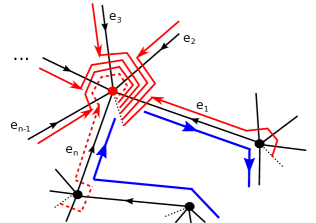
Figure 13: A face loop (blue) based at a ciliated vertex of $\Gamma$ (red), the paths $p_{e_{1},+}$, …, $p_{e_{n-1},+}$ (solid red) and the path $p_{e_{n},-}$ (dashed red) for the incident edges $e_{1},...,e_{n}$.

After clarifying the relation between gauge transformations in the two models, we can now relate curvatures in a Hopf algebra gauge theory on $\Gamma$ to the curvatures in the associated Kitaev model. As discussed in Section 4, the curvatures of a Hopf algebra gauge theory on a regular ciliated ribbon graph $\Gamma$ are given by the holonomies of ciliated faces that start and end at a cilia of $\Gamma$. Similarly, it was shown in Section 6.2 that the curvatures in the Kitaev models are given by the holonomies of the associated vertex loops and face loops in its thickening ${\Gamma_{D}}$ that start and end at these cilia. The isomorphism $\chi:\mathcal{A}^{*}_{\Gamma}\to\mathcal{H}(H)^{op\otimes E}$ from Theorem 7.3 relates the former to the latter.

Proposition 8.2.

Let $\Gamma$ be a regular ciliated ribbon graph, $v$ a vertex of $\Gamma$, $f(v)$ the ciliated face that starts and ends at the cilium at $v$ and $p_{v}$, $p_{f(v)}$ the associated vertex and face loops. Then

$$\chi\circ\mathrm{Hol}^{\Gamma}_{f(v)}(y\otimes\gamma)=\mathrm{Hol}^{{\Gamma_{D}}}_{p_{v}}(y\otimes 1)\cdot\mathrm{Hol}^{{\Gamma_{D}}}_{p_{f(v)}}(1\otimes\gamma)\qquad\forall y\in H,\gamma\in H^{*},$$

and the projectors $P_{f}:\mathcal{A}^{*}_{\Gamma}\to\mathcal{A}^{*}_{\Gamma}$ and $Q_{v}:\mathcal{H}(H)^{\otimes E}\to\mathcal{H}(H)^{\otimes E}$ from Lemma 4.8 and 6.3 satisfy

$$\chi\circ P_{f(v)}=Q_{v}\circ\chi.$$

Proof.

Denote by $\cdot$ the multiplication of $\mathcal{H}(H)^{\otimes E}$ and by $\cdot_{\mathcal{A}^{*}}$ the multiplication of $\mathcal{A}^{*}_{\Gamma}$. Suppose the ciliated face $f(v)\in\mathcal{G}(\Gamma)$ is given by the reduced word $f(v)=e_{1}^{\epsilon_{1}}\circ...\circ e_{n}^{\epsilon_{n}}$ with $e_{i}\in E(\Gamma)$ and $\epsilon_{i}\in\{\pm 1\}$. As $f(v)$ traverses each edge $e_{i}$ at most once, its holonomy is given by

$$\mathrm{Hol}^{\Gamma}_{f(v)}(y\otimes\gamma) =(S^{\tau_{1}}_{D}((y\otimes\gamma)_{(1)})\otimes S^{\tau_{2}}_{D}((y\otimes\gamma)_{(2)})\otimes...\otimes S^{\tau_{n}}_{D}((y\otimes\gamma)_{(n)}))_{e_{1}...e_{n}},$$

where $2\tau_{i}=1-\epsilon_{i}$. As $f(v)$ turns maximally right at each vertex and does not traverse any cilia, the edges $e_{i}$ and $e_{i+1}$ are adjacent at the vertex ${\bf t}(e_{i+1}^{\epsilon_{i+1}})={\bf s}(e_{i}^{\epsilon_{i}})$ with $e_{i+1}<e_{i}$ for all $i\in\{1,...,n-1\}$. As $f(v)$ starts and ends at the cilium at $v$, the edge $e_{n}$ is the edge of lowest and the edge $e_{1}$ the edge of highest order at $v$, as shown in Figure 14. Because $\Gamma$ has no loops or multiple edges, it follows from Proposition 4.4 that $(y\otimes\gamma\otimes z\otimes\delta)_{e_{i}e_{j}}=(z\otimes\delta)_{e_{j}}\cdot_{\mathcal{A}^{*}}(y\otimes\gamma)_{e_{i}}$ for all $1\leq i<j\leq n$. Because $f(v)$ traverses each edge of $\Gamma$ at most once, this implies

$$\mathrm{Hol}^{\Gamma}_{f(y)}(y\otimes\gamma)=(S^{\tau_{n}}_{D}((y\otimes\gamma)_{(n)}))_{e_{n}}\cdot_{\mathcal{A}^{*}}...\cdot_{\mathcal{A}^{*}}(S^{\tau_{2}}_{D}((y\otimes\gamma)_{(2)}))_{e_{2}}\cdot_{\mathcal{A}^{*}}(S^{\tau_{1}}_{D}((y\otimes\gamma)_{(1)}))_{e_{1}}.$$

As $\chi:\mathcal{A}^{*}_{\Gamma}\to\mathcal{H}(H)^{op\otimes E}$ is an algebra isomorphism with $\chi\circ\iota_{e}=\mathrm{Hol}^{\Gamma_{D}}_{p_{e,\pm}}$ and $\mathrm{Hol}^{{\Gamma_{D}}}_{p_{e,\pm}}\circ S_{D}=\mathrm{Hol}^{{\Gamma_{D}}}_{p_{e^{-1},\pm}}$ for all edges $e$ of $\Gamma$, this implies

$$\chi\circ\mathrm{Hol}^{\Gamma}_{f(v)}(y\otimes\gamma)=\mathrm{Hol}^{{\Gamma_{D}}}_{p_{e_{1}^{\epsilon_{1}},\pm}}((y\otimes\gamma)_{(1)})\cdot...\cdot\mathrm{Hol}^{{\Gamma_{D}}}_{p_{e_{n}^{\epsilon_{n}},\pm}}((y\otimes\gamma)_{(n)}),$$ (38)

where $p_{e,\pm}$ are the paths from Definition 7.1:

$$p_{e_{i}^{\epsilon_{i}}+}=p_{t(e_{i}^{\epsilon_{i}})<}\circ r(\bar{e}_{i}^{\epsilon_{i}})\circ r(e_{i}^{\epsilon_{i}})\circ p_{s(e_{i}^{\epsilon_{i}})<}^{-1}=:{t_{i}}\circ r(e_{i}^{\epsilon_{i}})\circ s_{i}^{-1}.$$

As $e_{i}$ and $e_{i+1}$ are adjacent at the vertex ${\bf t}(e_{i+1}^{\epsilon_{i+1}})={\bf s}(e_{i}^{\epsilon_{i}})$ with $e_{i+1}<e_{i}$ for $i\in\{1,...,n-1\}$ and $e_{n}$ and $e_{1}$ are the edges of lowest and highest order at $v$, respectively, one has $s_{i}=t_{i+1}$ for all $i\in\{1,...,n-1\}$, ${s_{n}}=\o_{v}$, $t_{1}=p_{v}$ and $p_{f(v)}=r(e_{1}^{\epsilon_{1}})\circ...\circ r(e_{n}^{\epsilon_{n}})$, as shown in Figure 14. Inserting these identities into (38) one obtains

$$\chi\circ\mathrm{Hol}^{\Gamma}_{f(v)}(y\otimes\gamma) =\mathrm{Hol}^{\Gamma_{D}}_{t_{1}}((y\otimes\gamma)_{(1)(1)})\cdot\mathrm{Hol}^{{\Gamma_{D}}}_{r(e_{1}^{\epsilon_{1}})}((y\otimes\gamma)_{(1)(2)})\cdot\mathrm{Hol}^{\Gamma_{D}}_{s_{1}^{-1}}((y\otimes\gamma)_{(1)(3)})$$

$$\;\;\cdot\mathrm{Hol}^{\Gamma_{D}}_{t_{2}}((y\otimes\gamma)_{(2)(1)})\cdot\mathrm{Hol}^{{\Gamma_{D}}}_{r(e_{2}^{\epsilon_{2}})}((y\otimes\gamma)_{(2)(2)})\cdot\mathrm{Hol}^{\Gamma_{D}}_{s_{2}^{-1}}((y\otimes\gamma)_{(2)(3)})$$

$$\;\;\quad\vdots$$

$$\;\;\cdot\mathrm{Hol}^{\Gamma_{D}}_{t_{n}}((y\otimes\gamma)_{(n)(1)})\cdot\mathrm{Hol}^{{\Gamma_{D}}}_{r(e_{n}^{\epsilon_{n}})}((y\otimes\gamma)_{(n)(2)})\cdot\mathrm{Hol}^{\Gamma_{D}}_{s_{n}^{-1}}((y\otimes\gamma)_{(2)(n)})$$

$$=\mathrm{Hol}^{{\Gamma_{D}}}_{p_{v}}(y\otimes 1)\cdot\mathrm{Hol}^{{\Gamma_{D}}}_{p_{f(v)}}(1\otimes\gamma),$$

where we used that the last holonomy in each line cancels with the first in the next one, because $s_{i}=t_{i+1}$, that the first holonomy is equal to the holonomy of $p_{v}$ and that the last one is trivial. The remaining holonomies combine to form the holonomy of $p_{f(v)}$. This implies for all $X\in\mathcal{A}^{*}_{\Gamma}$

$$\chi\circ P_{f(v)}(X) =\chi(\mathrm{Hol}^{\Gamma}_{f(v)}(\ell\otimes\eta)\cdot X)=\chi(X)\cdot\mathrm{Hol}^{{\Gamma_{D}}}_{p_{v}}(\ell\otimes 1)\cdot\mathrm{Hol}^{{\Gamma_{D}}}_{p_{f(v)}}(1\otimes\eta)=Q_{v}\circ\chi(X).$$

∎

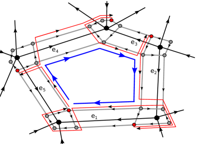
Figure 14: The paths $p_{e_{i},\pm}$ in ${\Gamma_{D}}$ for the ciliated face $f(v)=e_{1}\circ e_{2}\circ e_{3}^{-1}\circ e_{4}\circ e_{5}^{-1}$ .

In particular, Proposition 8.2 shows that projecting out the curvature of the ciliated face $f(v)$ in the Hopf algebra gauge theory amounts to projecting out the curvatures of both, the ciliated faces $p_{v}$ and $p_{f(v)}$, in the Kitaev model. This allows one to relate the projectors on the subalgebras of gauge invariant functions on flat gauge fields in the two models.

By composing the projectors $P_{f(v)}:\mathcal{A}^{*}_{\Gamma}\to\mathcal{A}^{*}_{\Gamma}$ from Lemma 4.8 for all vertices $v$ of a regular ribbon graph $\Gamma$ and restricting them to the gauge invariant subalgebra $\mathcal{A}^{*}_{\Gamma\,inv}\subset\mathcal{A}^{*}_{\Gamma}$, one obtains the projector $P_{flat}:\mathcal{A}^{*}_{\Gamma\,inv}\to\mathcal{A}^{*}_{\Gamma\,inv}$ from Theorem 4.9. Its image is the quantum moduli algebra $\mathcal{M}_{\Gamma}\subset\mathcal{A}^{*}_{\Gamma}$, which is a topological invariant and can be interpreted as the algebra of gauge invariant functions on the linear subspace of flat gauge fields.

Similarly, composing the projectors $Q_{v}:\mathcal{H}(H)^{\otimes E}\to\mathcal{H}(H)^{\otimes E}$ from Lemma 6.3 for all vertices $v$ of $\Gamma$ and restricting them to the gauge invariant subalgebra $\mathcal{H}(H)^{\otimes E}_{inv}$ yields the projector $Q_{flat}:\mathcal{H}(H)^{\otimes E}_{inv}\to\mathcal{H}(H)^{\otimes E}_{inv}$ from Lemma 6.3. Its image, the subalgebra $\mathcal{H}(H)^{\otimes E}_{flat}\subset\mathcal{H}(H)^{\otimes E}_{inv}$, can be interpreted as the algebra of operators acting on the protected space and contains those elements $X\in\mathcal{H}(H)^{\otimes E}$ with $H_{\mathrm{K}}\cdot X\cdot H_{\mathrm{K}}=X$. As the protected space is a topological invariant, the same holds for the algebra $\mathcal{H}(H)^{\otimes E}_{flat}$. With Proposition 8.2 it then follows that $\chi$ induces an algebra isomorphism between this algebra and the quantum moduli algebra of the Hopf algebra gauge theory and hence relates the topological invariants of the two models.

Theorem 8.3.

Let $\Gamma$ be a regular ciliated ribbon graph. Then $\chi:\mathcal{A}^{*}_{\Gamma}\to\mathcal{H}(H)^{op\otimes E}$ induces an algebra isomorphism $\chi:\mathcal{M}_{\Gamma}\to\mathcal{H}(H)^{op\otimes E}_{flat}$.

Proof.

By Theorem 4.9 and Lemma 6.3, the subalgebras $\mathcal{M}_{\Gamma}\subset\mathcal{A}^{*}_{\Gamma\,inv}$ and $\mathcal{H}(H)^{op\otimes E}_{flat}\subset\mathcal{H}(H)^{op\otimes E}_{inv}$ are the images of the projectors

$$P_{flat}=\Pi_{f\in F}P_{f}:\mathcal{A}^{*}_{\Gamma\,inv}\to\mathcal{A}^{*}_{\Gamma\,inv}\qquad Q_{flat}=\Pi_{v\in V}Q_{v}:\mathcal{H}(H)^{op\otimes E}_{inv}\to\mathcal{H}(H)^{op\otimes E}_{inv},$$

and all projectors $P_{f}$ and $Q_{v}$ commute. By Theorem 8.1 the map $\chi:\mathcal{A}^{*}_{\Gamma\,inv}\to\mathcal{H}(H)^{op\otimes E}_{inv}$ is an algebra isomorphism, and by Proposition 8.2 one has $\chi\circ P_{f(v)}=Q_{v}\circ\chi$ for all vertices $v\in V$. As $\Gamma$ is regular, the faces of $\Gamma$ are in bijection with the ciliated faces $f(v)$ based at the cilia of the vertices $v\in V$. This implies $\chi\circ P_{flat}=Q_{flat}\circ\chi$, and the claim follows. ∎

Theorems 8.1 and 8.3 also allow one to understand excitations in the Kitaev model from the viewpoint of Hopf algebra gauge theory. Creating an excitation in a Kitaev model at a site $(v,f(v))$ corresponds to removing the associated vertex operator $A_{v}^{\ell}$ and face operator $B^{\eta}_{f(v)}$ from the Hamiltonian $H_{\mathrm{K}}$. On the level of triangle operators, this amounts to removing the gauge transformations at the vertex $v$ from the projector $Q_{inv}$ in Lemma 6.2 and the projector $Q_{v}$ from the projector $Q_{flat}$ in Lemma 6.3. By Theorem 8.1 and Theorem 8.3, this is equivalent to removing the projector $P_{v}$ from the projector $P_{inv}$ in Theorem 4.5 and removing the projector $P_{f(v)}$ from the projector $P_{flat}$ in Theorem 4.9. Hence, from the viewpoint of Hopf algebra gauge theory, excitations are created by relaxing gauge invariance at a vertex $v$ of $\Gamma$ and flatness at the associated face $f(v)$.

Together, Theorems 7.6, 8.1 and 8.3 establish the full equivalence of a $D(H)$-valued Hopf algebra gauge theory on a regular ribbon graph $\Gamma$ and the associated Kitaev model for $H$. Theorem 7.6 shows that there is an algebra isomorphism between the algebra of functions of the Hopf algebra gauge theory and the algebra of triangle operators in the Kitaev model. Theorem 8.1 shows that this algebra isomorphism is compatible with the action of gauge transformations at the vertices of $\Gamma$ and hence induces an isomorphism between the subalgebras of gauge invariant functions in the two models. Proposition 8.2 then establishes that this isomorphism maps curvatures in the Hopf algebra gauge theory to curvatures in the Kitaev model. As the curvatures in the Hopf algebra gauge theory define a $C(D(H))^{\otimes F}$-module structure on the gauge invariant subalgebra by Lemma 4.7 and one has $C(D(H))\cong Z(D(H))$ and $|F|=|V|$, this defines $Z(D(H))^{\otimes V}$-module structures on the gauge invariant subalgebras of the two models. From Theorem 8.3 we then obtain an algebra isomorphism between the associated subalgebras of invariants. These are the topological invariants of the models, the quantum moduli algebra $\mathcal{M}_{\Gamma}$ of the Hopf algebra gauge theory and the algebra $\mathcal{H}(H)^{op\otimes E}_{flat}$ of operators on the protected space in the Kitaev model.

Denoting by $\mathcal{G}=D(H)^{\otimes V}$ the Hopf algebra of gauge transformations and by $\mathcal{C}=Z(D(H))^{\otimes V}$ the algebra of curvatures, we can describe the relation between Hopf algebra gauge theory and Kitaev models by the following commuting diagram that summarises the results of this article:

Acknowledgements. I thank Derek Wise and John Baez for discussions. This work was supported by the Action MP1405 QSPACE from the European Cooperation in Science and Technology (COST).

References

- [1] A. Alekseev, H. Grosse, V. Schomerus, Combinatorial quantization of the Hamiltonian Chern-Simons theory I, Commun. Math. Phys. 172.2 (1995) 317–358.
- [2] A. Alekseev, H. Grosse, V. Schomerus, Combinatorial quantization of the Hamiltonian Chern-Simons theory II, Commun. Math. Phys. 174.3 (1996) 561–604.
- [3] A. Alekseev, V. Schomerus, Representation theory of Chern-Simons observables, Duke Math. J. 85.2 (1996) 447–510.
- [4] A. Alekseev, A. Malkin, Symplectic structures associated to Lie-Poisson groups, Commun. Math. Phys. 162.1 (1994) 147-173.
- [5] B. Balsam, A. Kirillov Jr, Kitaev’s Lattice Model and Turaev-Viro TQFTs, arXiv preprint arXiv:1206.2308.
- [6] B. Balsam, Turaev-Viro invariants as an extended TQFT II, arXiv preprint arXiv:1010.1222.
-
[7]
B. Balsam, Turaev-Viro invariants as an extended TQFT III, arXiv preprint
arXiv:1012.0560. - [8] J. Barrett, Quantum gravity as topological quantum field theory, J. Math. Phys. 36.11 (1995) 6161-6179.
- [9] J. Barrett, J. Martins, J. García-Islas, Observables in the Turaev-Viro and Crane-Yetter models, J. Math. Phys. 48.9 (2007) 093508.
- [10] J. Barrett, B. Westbury, Invariants of piecewise-linear 3-manifolds, T. Am. Math. Soc. 348.10 (1996) 3997–4022.
- [11] W. Baskerville, S. Majid, The braided Heisenberg group, J. Math. Phys. 34.8 (1993) 3588–3606.
- [12] M. Beverland, O. Buerschaper, R. Koenig, F. Pastawski, J. Preskill, S. Sijher, Protected gates for topological quantum field theories, J. Math. Phys., 57(2) (2016) 022201.
- [13] H. Bombin, M. Martin-Delgado, A Family of non-Abelian Kitaev models on a lattice: Topological condensation and confinement, Phys. Rev. B 78.11 (2008) 115421.
- [14] O. Buerschaper, M. Aguado, Mapping Kitaev’s quantum double lattice models to Levin and Wen’s string-net models, Phys. Rev. B 80.15 (2009) 155136.
- [15] O. Buerschaper, J. M. Mombelli, M. Christandl, M. Aguado, A hierarchy of topological tensor network states, J. Math. Phys. 54.1 (2013) 012201.
- [16] E. Buffenoir, K. Noui, Ph. Roche, Hamiltonian Quantization of Chern-Simons theory with Group, Class. Quant. Grav. 19 (2002) 4953–5016.
- [17] E. Buffenoir, Ph. Roche, Two dimensional lattice gauge theory based on a quantum group, Commun. Math. Phys. 170.3 (1995) 669–698.
- [18] E. Buffenoir, Ph. Roche, Link invariants and combinatorial quantization of hamiltonian Chern Simons theory, Commun. Math. Phys. 181.2 (1996) 331–365.
- [19] D. Bullock, C. Frohman, J. Kania-Bartoszýnska, Topological Interpretations of Lattice Gauge Field Theory, Commun. Math. Phys. 198, (1998) 47–81.
- [20] V. Drinfeld, On Almost Cocommutative Hopf Algebras, Len. Math. J. 1 (1990), 321–342.
- [21] J. Ellis-Monaghan, I. Moffat, Graphs on surfaces: dualities, polynomials, and knots, Vol. 84 (2013) Springer, Berlin.
- [22] P. Etinghof, S. Gelaki, Some properties of finite-dimensional semisimple Hopf algebras, Math. Res. Lett. 5 (1998) 191–197.
- [23] V. Fock, A. Rosly, Poisson structure on moduli of flat connections and r-matrix, Am. Math. Soc. Transl. 191 (1999) 67–86.
- [24] Z. Kádár, A. Marzuoli, M. Rasetti, Microscopic description of 2d topological phases, duality, and 3D state sums, Adv. Math. Phys, 2010, Article ID 671039, 18 pages.
- [25] Z. Kádár, A. Marzuoli, M. Rasetti, Braiding and entanglement in spin networks: a combinatorial approach to topological phases, Int. J. Quantum Inf. 7.supp (2009) 195–203.
- [26] C. Kassel, Quantum groups, Vol. 155 (2012) Springer Science & Business Media.
- [27] A. Kirillov Jr, B. Balsam, Turaev-Viro invariants as an extended TQFT, arXiv preprint arXiv:1004.1533.
- [28] A. Kitaev, Fault-tolerant quantum computation by anyons, Ann. Phys. 303.1 (2003) 2–30.
-
[29]
A. Kitaev, L. Kong, Models for gapped boundaries and domain walls, Commun. Math.
Phys. 313.2 (2012) 351–373. - [30] R. Koenig, G. Kuperberg, B. Reichardt, Quantum computation with Turaev-Viro codes, Ann. Phys. 325.12 (2010) 2707–2749.
- [31] S. Lando, A. Zvonkin, Graphs on surfaces and their applications, Vol. 141 (2013) Springer Science & Business Media.
- [32] G. Larson, D. Radford, Semisimple Cosemisimple Hopf Algebras, Am. J. Math. 109 (1987), 187–195.
- [33] M. Levin, X.-G. Wen, String-net condensation: a physical mechanism for topological phases, Phys. Rev. B 71.4 (2005) 045110.
- [34] M. Levin, X.-G. Wen, Detecting topological order in a ground state wave function, Phys. Rev. Lett. 96.11 (2006) 110405.
- [35] S. Majid, Algebras and Hopf algebras in braided categories, in: Advances in Hopf algebras, Lecture Notes in Pure and Appl. Math 158, Dekker, New York (1994) 55–105.
- [36] S. Majid, Foundations of quantum group theory (2000) Cambridge University Press.
- [37] C. Meusburger, K. Noui, The Hilbert space of 3d gravity: quantum group symmetries and observables, Adv. Theor. Math. Phys. 14.6 (2010) 1651-1716.
- [38] C. Meusburger, D. Wise, Hopf algebra gauge theory on a ribbon graph, arXiv preprint arXiv:1512.03966.
- [39] S. Montgomery, Hopf algebras and their actions on rings (1993) Montgomery, American Mathematical Soc. 82.
- [40] D. Radford, Minimal quasitriangular Hopf algebras, J. Algebra 157.2 (1993) 281–315.
- [41] D. Radford, Hopf algebras, Series on Knots and everything 49 (2011) World Scientific.
- [42] N. Reshetikhin, V. Turaev, Invariants of 3-manifolds via link polynomials and quantum groups, Invent. Math. 103.1 (1991) 547–597.
- [43] V. Turaev, A. Virelizier, On two approaches to 3-dimensional TQFTs, arXiv preprint arXiv:1006.3501.
- [44] V. Turaev, O. Viro, State sum invariants of 3-manifolds and quantum 6j-symbols, Topology 31.4 (1992) 865–902.
- [45] E. Witten, Quantum field theory and the Jones polynomial, Commun. Math. Phys. 121.3 (1989) 351–399.