H0LiCOW III. Quantifying the effect of mass along the line of sight to the gravitational lens HE 04351223 through weighted galaxy counts ††thanks: Based on data collected at Subaru Telescope, which is operated by the National Astronomical Observatory of Japan.
Abstract
Based on spectroscopy and multiband wide-field observations of the gravitationally lensed quasar HE 04351223, we determine the probability distribution function of the external convergence for this system. We measure the under/overdensity of the line of sight towards the lens system and compare it to the average line of sight throughout the universe, determined by using the CFHTLenS as a control field. Aiming to constrain as tightly as possible, we determine under/overdensities using various combinations of relevant informative weighing schemes for the galaxy counts, such as projected distance to the lens, redshift, and stellar mass. We then convert the measured under/overdensities into a distribution, using ray-tracing through the Millennium Simulation. We explore several limiting magnitudes and apertures, and account for systematic and statistical uncertainties relevant to the quality of the observational data, which we further test through simulations. Our most robust estimate of has a median value and a standard deviation of . The measured corresponds to uncertainty on the time delay distance, and hence the Hubble constant inference from this system. The median value is robust to (i.e. on ) regardless of the adopted aperture radius, limiting magnitude and weighting scheme, as long as the latter incorporates galaxy number counts, the projected distance to the main lens, and a prior on the external shear obtained from mass modelling. The availability of a well-constrained makes HE 04351223 a valuable system for measuring cosmological parameters using strong gravitational lens time delays.
keywords:
gravitational lensing: strong – cosmological parameters – distance scale – methods: statistical – quasars: individual: HE 043512231 Introduction
By measuring time delays between the multiple images of a source with time-varying luminosity, strong gravitational lens systems with measured time delays can be used to measure cosmological distances and the Hubble constant (Refsdal, 1964). In particular, for a lens system with a strong deflector at a single redshift, one may infer the ‘time-delay distance’
| (1) |
where denotes the redshift of the foreground deflector, the angular diameter distance to the deflector, the angular diameter distance to the source, and the angular diameter distance between the deflector and the source. The time-delay distance is primarily sensitive to the Hubble constant, i.e. (see Treu & Marshall, 2016, for a recent review).
Inferring cosmological distances from measured time delays also requires accurate models for the mass distribution of the main deflector and its environment, as well as for any other matter structures along the line of sight that may influence the observed images and time delays (Suyu et al., 2010). Galaxies very close in projection to the main deflector often cause measurable higher-order perturbations in the lensed images and time delays and require explicit models of their matter distribution. The effect of galaxies more distant in projection is primarily a small additional uniform focusing of the light from the source. Furthermore, matter underdensities along the line of sight such as voids, indicated by a low galaxy number density, cause a slight defocusing. For a strong lensing system with a main deflector at a single redshift, the net effect of the (de)focusing by these weak perturbers is equivalent (to lowest relevant order) to that of a constant external convergence111The external convergence may be positive or negative depending on whether focusing or defocusing outweighs the other. term in the lens model for the main deflector (Suyu et al., 2010). This implies on the one hand that the weak perturbers’ effects, i.e. the external convergence they induce, cannot be inferred from the observed strongly lensed image properties alone due to the ‘mass-sheet degeneracy’ (MSD, Falco, Gorenstein, & Shapiro, 1985; Schneider & Sluse, 2013). On the other hand, if the external convergence is somehow determined from ancillary data, and a time-delay distance has been inferred using a model not accounting for the effects of weak perturbers along the line of sight, the true time-delay distance can simply be computed by:
| (2) |
This relation makes clear that any statistical and systematic uncertainties in the external convergence due to structures along the line of sight directly translate into statistical and systematic errors in the inferred time delay distance and Hubble constant:
| (3) |
where denotes the Hubble constant inferred when neglecting weak external perturbers. With reduced uncertainties on other component of the time delay distance measurement from state-of-the-art imaging, time-delay measurements, and modeling techniques of strong lens systems, the external convergence is now left as an important source of uncertainty on the inferred , contributing up to to the error budget on (Suyu et al., 2010, 2013). Moreover, the mean external convergence may not vanish for an ensemble of lens systems due to selection effects, causing a slight preference for lens systems with overdense lines of sights (Collett et al., 2016). Thus, an ensemble analysis simply assuming is expected to systematically overestimate the Hubble constant .
Accurately quantifying the distribution of mass along the line of sight requires wide-field imaging and spectroscopy (e.g., Keeton & Zabludoff, 2004; Fassnacht et al., 2006; Momcheva et al., 2006; Fassnacht, Koopmans, & Wong, 2011; Wong et al., 2011, see Treu & Marshall (2016) for a recent review). Suyu et al. (2010) pioneered the idea of estimating a probability distribution function by (i) measuring the galaxy number counts around a lens system, (ii) comparing the resulting counts against those of a control field to obtain relative counts, and (iii) selecting lines of sight of similar relative counts, along with their associated convergence values, from a numerical simulation of cosmic structure evolution. To this end, Fassnacht, Koopmans, & Wong (2011) measured the galaxy number counts in a aperture around HE 04351223 [(2000): 04h 38m 14.9s, (2000): -12∘17′144; Wisotzki et al., 2000, 2002; lens redshift ; Morgan et al., 2005; source redshift ; Sluse et al., 2012], and found that it is 0.89 of that on an average line of sight through their control field. Both Greene et al. (2013, hereafter G13) and Collett et al. (2013) find that can be most precisely constrained for lens systems along underdense lines of sight, making HE 04351223 a valuable system.
Recent work has focused on tightening the constraints on with data beyond simple galaxy counts. Suyu et al. (2013) used the external shear inferred from lens modelling as a further constraint, which significantly affected the inferred external convergence due to the large external shear required by the lens model. G13 extended the number counts technique by considering more informative, physically relevant weights, such as galaxy redshift, stellar mass, and projected separation from the line of sight. Both of these works used ray-tracing through the Millennium Simulation (Springel et al., 2005; Hilbert et al., 2009, hereafter MS) in order to obtain . For lines of sight which are either underdense or of common density, G13 found that the residual uncertainty on the external convergence can be reduced to , which corresponds to an uncertainty on time delay distance and hence comparable to that arising from the mass model of the deflector and its immediate environment. Furthermore, Collett et al. (2013) considered a reconstruction of the mass distribution along the line of sight using a galaxy halo model. They convert the observed environment around a lens directly into an external convergence, after calibrating for the effect of dark structures and voids by using the MS.
We have collected sufficient observational data to implement these techniques for the case of HE 04351223. We choose to adopt the G13 approach, with several improvements. We first aim to understand and account for various sources of error in our observational data for HE 04351223, as well as that of CFHTLenS (Heymans et al., 2012), which we choose as our control field. Second, we incorporate our understanding of these uncertainties into the simulated catalogues of the MS, in order to ensure a realistic estimate of . Third, we use the MS to test the robustness of this estimate for simulated fields of similar under/overdensity.
This paper is organized as follows. In Section 2 we present the relevant observational data for HE 04351223 and its reduction. In Section 3 we present an overview of our control field, CFHTLenS. In Section 4 we present our source detection, classification, photometric redshift and stellar mass estimation, carefully designed to match the CFHTLenS fields. In Section 5 we present our technique to measure weighted galaxy count ratios for HE 04351223, by accounting for relevant errors. In Section 6 we use ray-tracing through the MS in order to obtain for the measured ratios, and present our tests for robustness. We present and discuss our results in Section 7, and we conclude in Section 8. We present additional details in the Appendix.
The current work represents Paper III (hereafter H0LiCOW Paper III) in a series of five papers from the H0LiCOW collaboration, which together aim to obtain an accurate and precise estimate of from a comprehensive modelling of HE 04351223. An overview of this collaboration can be found in H0LiCOW Paper I (Suyu et al., submitted), and the derivation of is presented in H0LiCOW Paper V (Bonvin et al., submitted).
Throughout this paper, we assume the MS cosmology, , , , .222We estimate the impact of using a different cosmology in Section C. We present all magnitudes in the AB system, where we use the following conversion factor between the Vega and the AB systems: , and 333Results based on the MOIRCS filters, available at http://www.astro.yale.edu/eazy/filters/v8/FILTER.RES.v8.R300.info.txt. We define all standard deviations as the semi-difference between the 84 and 16 percentiles.
2 Data reduction and calibration
In order to characterize the HE 04351223 field, we require a catalogue of galaxy properties, such as galaxy redshifts and stellar masses. To this end, we have obtained multiband, wide-field imaging observations of HE 04351223, from ultraviolet to near/mid-infrared wavelengths. The observations are detailed in Table 1, and were obtained with the Canada-France-Hawaii Telescope (CFHT; PI. S. Suyu), the Subaru Telescope (PI. C. Fassnacht), and the Gemini North Telescope (PI. C. Fassnacht). We also use archival Spitzer Telescope data (PI. C. Kochanek, Program ID 20451). In addition, we make use of a number of secure spectroscopic redshifts (374 and 43 objects inside a and -radius circular aperture, respectively, not counting the lens itself), obtained with the Magellan 6.5m telescope Momcheva et al. (2006); Momcheva et al. (2015), the VLT (PI: Sluse), the Keck Telescope (PI: Fassnacht), and the Gemini Telescope (PI: Treu; see H0LiCOW Paper II for details on the spectroscopic observations). Those data provide a spectroscopic identification of 90% ( 60%) of the galaxies down to mag (mag) within a radius of of the lens, namely the maximum radius within which we calculate weighted number counts in this work (see Fig. 3 of H0LiCOW Paper II for spectroscopic completeness as a function of radius/magnitude).
| Telescope/Instrument | FOV []/scale [] | Filter | Exposure [sec] | Airmass | Seeing [] | Observation date |
|---|---|---|---|---|---|---|
| CFHT/MegaCam | /0.187 | 1. | 2014 Aug. 31 - Sep. 2 | |||
| Subaru/Suprime-Cam | /0.200 | 2014 Mar. 1 | ||||
| Subaru/Suprime-Cam | /0.200 | 2014 Mar. 1 | ||||
| Subaru/Suprime-Cam | /0.200 | 2014 Mar. 1 | ||||
| Gemini North/NIRI | /0.116 | 2012 Aug. 22 | ||||
| Subaru/MOIRCS | /0.116 | 2015 Apr. 1 | ||||
| Gemini North/NIRI | /0.116 | 2012 Aug. 22 | ||||
| Spitzer/IRAC | /0.6 | 3.6 | - | - | 2006 Feb. 8, 2006 Sep. 20 | |
| Spitzer/IRAC | /0.6 | 4.5 | - | - | 2006 Feb. 8, 2006 Sep. 20 | |
| Spitzer/IRAC | /0.6 | 5.8 | - | - | 2006 Feb. 8, 2006 Sep. 20 | |
| Spitzer/IRAC | /0.6 | 8.0 | - | - | 2006 Feb. 8, 2006 Sep. 20 |
For NIRI, where the instrument field of view is just , “FOV” refers to the effective field of view on the sky, after dithering. For IRAC, the filters denote the effective wavelengths in m.
We reduced the imaging data using standard reduction techniques. We obtained the CFHT MegaCam (Boulade et al., 2003) and Spitzer IRAC (Fazio et al., 2004) data already pre-reduced and photometrically calibrated. We used Scamp (Bertin, 2006) to achieve consistent astrometric and photometric calibration, and Swarp (Bertin et al., 2002) to resample the data on a pixel scale, using a tangential projection. This is the native pixel scale of Subaru Suprime-Cam (Kobayashi et al., 2000), and the largest among the available data, with the exception of IRAC ( pixel scale).
We reduced the Subaru MOIRCS (Suzuki et al., 2008; Ichikawa et al., 2006) data using a pipeline provided by Ichi Tanaka, based on IRAF444IRAF is distributed by the National Optical Astronomy Observatory, which is operated by the Association of Universities for Research in Astronomy (AURA) under cooperative agreement with the National Science Foundation.. For the Gemini NIRI (Hodapp et al., 2003) and Subaru MOIRCS data we calibrated the photometry using 2MASS stars in the field of view (FOV). For Subaru Suprime-Cam, we used observations of an SDSS star field, taken the same night. We excluded stars with nearby companions that can affect the SDSS photometry, and used color transformations provided by Yagi Masafumi (private communication; also described in Yagi et al. (2013a, b)), in order to calibrate the photometry to the AB system. We corrected for galactic and atmospheric extinction following Schlafly & Finkbeiner (2011) and Buton et al. (2012), respectively. We present our strategy for source detection, classification, redshift and stellar mass estimation, in Section 4.
3 The control field: CFHTLenS
In order to apply the weighted number counts technique, we need a control field against which to determine an under/overdensity. We require the field to be of a suitable depth, as well as larger in spatial extent than the field used by Fassnacht, Koopmans, & Wong (2011), or the Cosmic Evolution Survey (Scoville et al., 2007, COSMOS), which is known to be overdense (e.g., Fassnacht, Koopmans, & Wong, 2011, and references within). The field should consist of several fields spread across the sky, in order to account for sample variance, and should also contain high to medium resolution, well-calibrated multiband data for object classification, and to infer photometric redshifts and stellar masses reliably.
Such a field is provided by the wide component of the CFHT Legacy Survey (CFHTLS; Gwyn, 2012). It consists of imaging over four distinct contiguous fields: W1 ( deg2 ), W2 ( deg2 ), W3 ( deg2 ) and W4 ( deg2), with typical seeing in -band. The data have been further processed, and are available in catalogue form from CFHTLenS (Heymans et al., 2012). We provide here a summary of the CFHTLenS data quality and products that are relevant to our analysis. CFHTLenS reaches down to limiting magnitude in a aperture in the deepest band, (Erben et al., 2013). The photometry has been homogenized through matched and gaussianised point-spread functions (PSFs) (Hildebrandt et al., 2012), leading to well-characterized photometric redshifts. The CFHTLenS catalogue includes best-fit photometric redshifts derived with BPZ (Benítez, 2000), and best-fit stellar masses computed with Le PHARE (Ilbert et al., 2006). The final product has a spectroscopic to photometric redshift scatter of for ( for ). The outlier fraction555The outliers are defined as galaxies with is for ( for ) (Hildebrandt et al., 2012).
The object detection and measurement are summarized by Erben et al. (2013): SExtractor (Bertin & Arnouts, 1996) is run six times in dual-image mode. In five of the runs, the detection image is the deeper image band (), and the measurement images are the PSF-matched images in each of the five bands; in the sixth run, the measurement image is the original lensing band image. This last run is performed to obtain total magnitudes (SExtractor quantity MAG_AUTO) in the deepest band, whereas the first five runs yield accurate colours based on isophotal magnitudes (MAG_ISO).
The galaxy-star classification is summarized by Hildebrandt et al. (2012), who also estimate its uncertainty, quantified in terms of incompleteness and contamination, based on a comparison with spectroscopic data from the VVDS F02 (Le Fèvre et al., 2005, reaching down to mag) and VVDS F22 (Garilli et al., 2008) surveys. In brief, for , objects with size smaller than the PSF are classified as stars. For , all objects are classified as galaxies. In the range , an object is defined as a star if its size is smaller than the PSF, and in addition , where is the best-fitting goodness-of-fit from the galaxy and star libraries given by Le PHARE.
4 Measuring physical properties of galaxies
4.1 Detecting and measuring sources with SExtractor
In order to avoid introducing biases in measuring weighted number counts, it is important to adopt detection, measuring and classification techniques for the HE 04351223 field that are as close as possible to those of CFHTLenS, while also assessing the similarities between the two datasets.
The HE 04351223 data are similar in terms of seeing to those from CFHTLenS (Table 1). The pixel scales of the two datasets differ by only . In terms of depth, the limiting magnitude of the HE 04351223 data in -band, following the definition in Erben et al. (2013)666, where ZP is the magnitude zero-point, is the number of pixels in a circle with radius 2.0″, and is the sky-background noise variation. We derive the uncertainty as the standard deviation of the values in 10 empty regions across the frame., is , thus virtually indistinguishable from the counterpart band in CFHTLenS (Section 3). The limiting magnitudes in the other bands are, respectively, (), (), (), (), (), (), and can be compared with the available counterparts in Table 1 of Erben et al. (2013). In particular, our deepest image (-band) is mag deeper than the CFHTLenS -band.
To infer accurate photometry, we matched the PSFs in the images to that in the band, which has the largest seeing. We combined bright, unsaturated stars across the field of view in each band, in order to build their PSFs. We replaced the noisy wings with analytical profiles, and computed convolution kernels using the Richardson-Lucy deconvolution algorithm (Richardson, 1972; Lucy, 1974).
Our primary region of interest is a area around HE 04351223 , as for this area we have (for the most part) uniform coverage in all bands, including IRAC. However, it is important to also consider a larger area, in order to use as many spectroscopically observed galaxies as possible for calibrating photometric redshifts. In addition, a wider area is necessary for identifying groups/clusters (H0LiCOW Paper II), and performing a weak lensing analysis (Tihhonova et al., in prep.). As a result, we are also interested in the whole coverage of the frames.
Before using SExtractor in a similar way to CFHTLenS on the images, we masked bright stars that are heavily saturated in -band. We found that by fitting and subtracting a Moffat profile to these bright stars, we can reduce the contamination of nearby objects by the bright stars, and improve the detection parameters; this minimizes the area that needs to be masked in the -band, but which is unaffected in most of the other bands. We convolve the masks with a narrow gaussian, in order smooth their edges, which would otherwise produce spurious detections. We also set a mask of radius around the HE 04351223 system itself, in order to account for the fact that the external convergence of the most nearby galaxy is accounted for explicitly in the lens mass modeling in H0LiCOW Paper IV (Wong et al., submitted).
Despite our -band being deeper, given the fact that CFHTLenS performed detections in , and the similarity of our band frame to the CFHTLenS -band, we first performed detections in the unconvolved (pre-PSF matching) image. For this, we ran SExtractor with the same detection parameters used by CFHTLenS (Jean Coupon, private communication). The purpose of this run is to estimate total magnitudes MAG_AUTO in this band, which we use when performing magnitude cuts at our faint threshold. However, for the purpose of extracting reliable photometry to be used for photometric redshift and stellar mass estimation, since measurements are expected to be more reliable in -band (with an exception being around bright objects, which appear brighter than in ), we also perform detections in this band, using optimized SExtractor detection parameters. As for measurements, we perform them as described for CFHTLenS in Section 3. We infer final MAG_ISO magnitudes, corrected for total magnitude, following CFHTLenS, as MAG_ISOx + (MAG_AUTOr MAG_ISOr), where the subscript refers to the measurement band (). We make an exception for of objects, which have a SExtractor flag indicative of unreliable MAG_AUTO, and for which we use replace MAG_AUTO with MAG_ISO instead. For the FOV outside , which is used for separate purposes by H0LiCOW Paper II and Tihhonova et al., in prep. we performed all detections in the -band only. We find that galaxies with mag are typically detected in all bands, with the exception of in , where the spatial coverage is also reduced, and in -band.
We use T-PHOT (Merlin et al., 2015) to extract MAG_ISO magnitudes, and thus measure colors between optical and IRAC filters, as the latter have vastly different pixel scale and PSFs. For this, we use the -band image as position and morphology prior. Finally, we apply the same star-galaxy classification used by CFHTLenS.
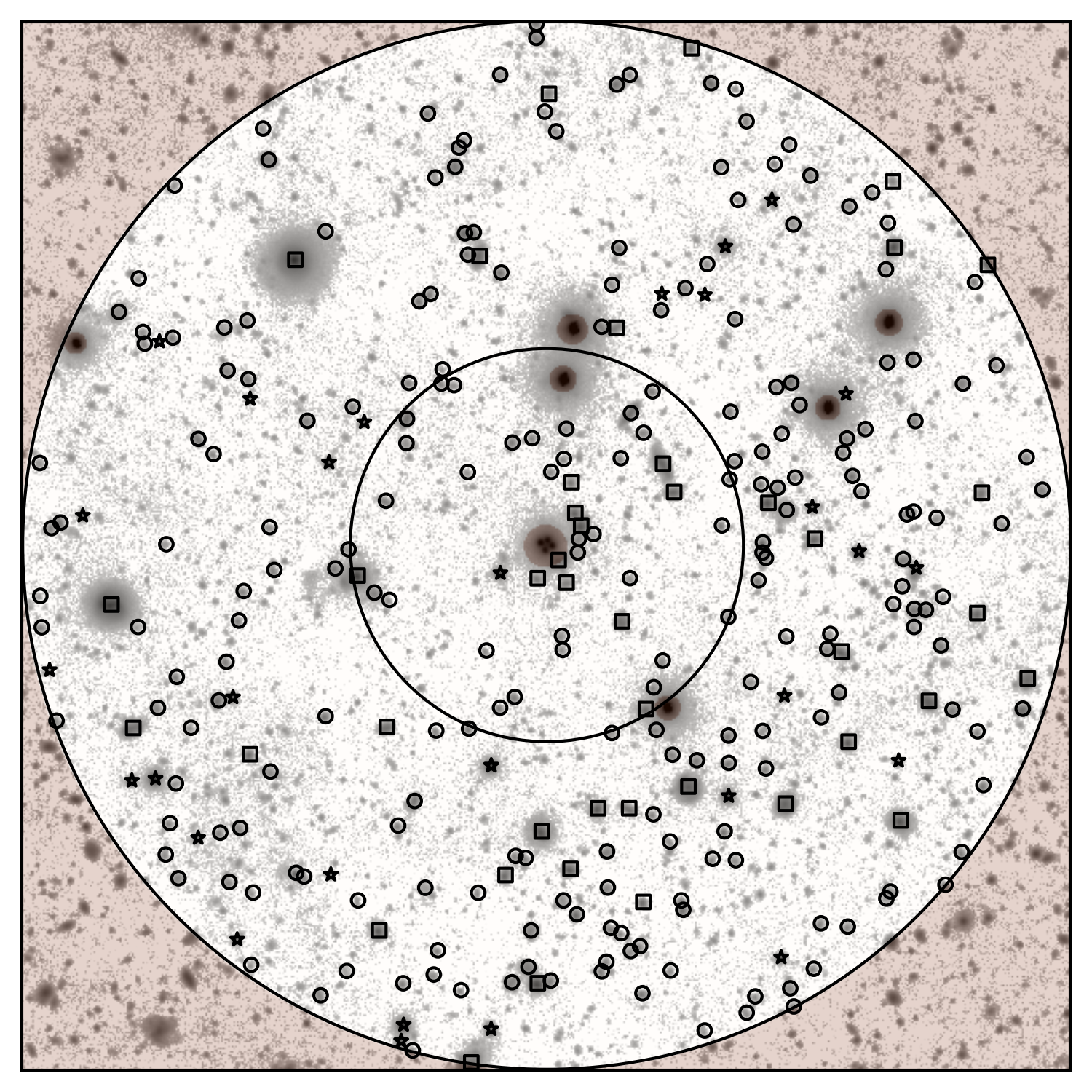
Table LABEL:tab:phot compiles the galaxies detected in a -radius aperture around HE 04351223, along with their measured photometry. The galaxies in a -radius aperture can be found in the accompanying online material, and are marked on the color-combined image in Figure 1.
4.2 Galaxy-star separation, redshifts and stellar masses
Using the PSF-matched photometry measured with SExtractor, we infer photometric redshifts and stellar masses, which we will later use as weights. We further calibrate our magnitudes by finding the zero points which minimize the scatter between photometric and spectroscopic redshifts of the mag galaxies with available spectroscopy. Finally, we perform a robust galaxy-star classification using morphological as well as photometric information. For measuring redshifts, we primarily use BPZ, which was also employed by CFHTLenS. However, we also use EAZY (Brammer, van Dokkum, & Coppi, 2008), to assess the dependence on a particular code/set of templates.
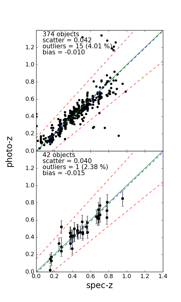
For the purpose of estimating photometric redshifts we ignore the IRAC channels, as e.g. Hildebrandt et al. (2010) note that the use of currently available mid-IR templates degrade rather than improve the quality of the inferred redshifts. For both BPZ and EAZY, we obtained the best results when using the default set of templates (CWW+SB and a linear combination of principal component spectra, respectively), with the default priors. Figure 2 compares the available spectroscopic redshifts with the inferred photometric redshift for the and filters, and galaxies with mag. There is negligible bias, and the scatter/outlier fractions are comparable to or smaller than the ones for CFHTLenS (Section 3). In addition, Figure 15 compares the BPZ- and EAZY-estimated redshifts, for the galaxies inside the region around HE 04351223, showing a good overall match.
For estimating stellar masses, we followed the approach by Erben et al. (2013), which was also used to produce the CFHTLenS catalogues. This uses templates based on the stellar population synthesis package of Bruzual & Charlot (2003), with a Chabrier (2003) initial mass function (see Velander et al. (2014) for additional details), and fits stellar masses with Le PHARE, at fixed redshift. We performed the computation twice, without and with using the IRAC photometry. In the latter case, we boosted the photometric errors to account for the template error derived by Brammer, van Dokkum, & Coppi (2008). We find only small scatter ( in ) and no bias, in agreement with the results of Ilbert et al. (2010) for a similar redshift range. The resulting redshifts and the stellar masses are given in Table LABEL:tab:zmstar. We used the median of the mass probability distribution as our estimate, except for a few percent of galaxies where Le PHARE fails to give a physical estimate for this, and we use the best-fit value instead. This is also the case for the CFHTLenS catalogues, where we recomputed stellar masses in order to fix the of objects with missing estimates. In fact, we recomputed stellar masses for the whole CFHTLenS catalogues, in order to use the same cosmology employed by the MS.
Finally, following the recipe from Section 3, we performed a galaxy-star classification. As described in more detail by Hildebrandt et al. (2012), we estimated the PSF size as the upper cut half light radius estimated by SExtractor in -band, and we used all available bands when computing the goodness-of-fit. Comparing to the available spectroscopic data, we find that all spectroscopically-confirmed galaxies are correctly classified as galaxies, whereas three spectroscopically-confirmed stars, with blended galaxy contaminants, are incorrectly classified as galaxies. We therefore removed them.
5 Determining line-of-sight under/overdensities using weighted number counts
5.1 Description of the technique
Fassnacht, Koopmans, & Wong (2011) computed lens field overdensities as galaxy count ratios, by first measuring the mean number counts in a given aperture through their control field, and then dividing the counts in the same aperture around the lens to the mean, i.e. . The situation is more complicated for us, because 1) we are interested in using weights dependent on the particular galaxy position inside the aperture, and 2) the CFHTLenS control fields contain a large fraction of masks throughout. These masked areas are due to luminous halos around saturated stars, asteroid trails, flagged pixels etc. (Erben et al., 2013).
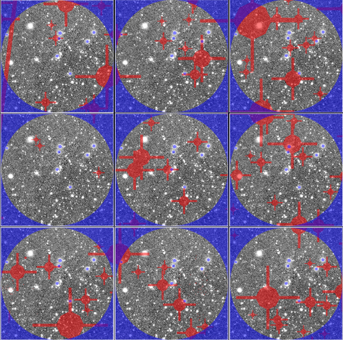
Therefore, to implement our galaxy weighting schemes, we first divide each of each of the W1-W4 CFHTLenS fields into a two-dimensional, contiguous grid of cells, of the same size as the apertures we consider around HE 04351223. We apply the CFHTLenS masks, at their particular position inside the cell, to the HE 04351223 field as well. Thus, when measuring weighted counts, we test whether each galaxy in the HE 04351223 field is located at a position which is covered by a mask in a particular cell. Conversely, we also test whether a galaxy in the cell is covered by a mask in the HE 04351223 field. This technique is depicted in Figure 3.
We divide the weighted counts measured around HE 04351223 to those measured in the same way around the center of each of the cells in the CFHTLenS grid, and consider the median of these divisions as our estimate of the overdensity. We justify the use of the median in Section 5.2 and Appendix B. Formally, then becomes , where and spans the number of cells in a CFHTLenS field. Following the notation in G13, we generalize from number counts to weighted counts by replacing with , where refers to a particular type of weight. Therefore generalizes to .
Following G13 we adopt these weights: , i.e. simple galaxy counting; , i.e. summing up powers of galaxy stellar masses; and . In addition, we also consider weights incorporating the distance to the lens/center of the field: , , and , as well as the weighted counts and .
In addition to the weights from G13, we define an additional weight, , where corresponds to the tidal and the flexion shift, respectively, of a point mass, as defined in McCully et al. (2016). We have simplified the definition of these two quantities, by removing the explicit redshift dependence. This is because the lensing convergence maps of the MS are not designed to account for this dependence (Hilbert et al., 2009). Another weight, , corresponds to the convergence produced by a singular isothermal sphere. We supplement this with a final related weight, , where stands for the halo mass of the galaxy, derived from the stellar mass by using the relation of Behroozi, Conroy, & Wechsler (2010).
| RA | DEC | ||||||||||||
| 69.57430 | 18.64 | ||||||||||||
| 69.55442 | 20.12 | ||||||||||||
| 69.55975 | 20.21 | ||||||||||||
| 69.56122 | 20.43 | ||||||||||||
| 69.55652 | 20.73 | ||||||||||||
| 69.56013 | 21.03 | ||||||||||||
| 69.55710 | 21.04 | ||||||||||||
| 69.55370 | 21.19 | ||||||||||||
| 69.57109 | 21.24 | ||||||||||||
| 69.55553 | 21.67 | - | |||||||||||
| 69.56258 | 21.73 | ||||||||||||
| 69.56038 | 22.00 | ||||||||||||
| 69.56071 | 22.16 | ||||||||||||
| 69.57321 | 22.31 | - | - | ||||||||||
| 69.55510 | 22.73 | - | |||||||||||
| 69.55990 | 22.81 | ||||||||||||
| 69.55017 | 22.89 | - | |||||||||||
| 69.56423 | 22.93 | ||||||||||||
| 69.55569 | 22.96 | ||||||||||||
| 69.56407 | 22.98 | - |
The complete catalogue of galaxies inside is available as online material, and the photometry for the complete Subaru/Suprime-Cam FOV is available upon request. Galaxies covered by the masks in Figure 1, except for the nearest companion inside of HE 04351223, are not reported. Here is the SExtractor with detections in -band, and the rest are magnitudes with detections in the -band, corrected by adding . Reported magnitudes are corrected for atmospheric (when necessary) and galactic extinction, but not for the zero point offsets estimated by BPZ (with the exception of ; see text). These offsets are: , , , , , and . For the IRAC channels, errors include those from the EAZY template error function.
| RA | DEC | sep | zspec/bpz | RA | DEC | sep | zspec/bpz | |||||||||
| 69.57430 | 43.88 | 0.515 | - | - | 11.1500 | 14.0037 | 69.56258 | 7.87 | 0.781 | - | - | 10.5502 | 12.8158 | |||
| 69.55442 | 32.48 | 0.277 | - | - | 9.9580 | 12.1143 | 69.56038 | 15.47 | 0.702 | - | - | 10.4472 | 12.6788 | |||
| 69.55975 | 9.05 | 0.419 | - | - | 9.9445 | 12.1451 | 69.56071 | 9.71 | 0.779 | - | - | 10.7420 | 13.0907 | |||
| 69.56122 | 4.32 | 0.782 | - | - | 10.9000 | 13.3647 | 69.57321 | 40.96 | 0.48 | 0.41 | 0.55 | 9.2501 | 11.7876 | |||
| 69.55652 | 35.83 | 0.41 | 0.34 | 0.48 | 10.1380 | 12.2910 | 69.55510 | 42.73 | 0.36 | 0.29 | 0.43 | 9.3728 | 11.8225 | |||
| 69.56013 | 9.85 | 0.457 | - | - | 10.3990 | 12.5692 | 69.55990 | 7.47 | 0.64 | 0.56 | 0.72 | 9.3000 | 11.8362 | |||
| 69.55710 | 24.50 | 0.678 | - | - | 9.8689 | 12.1570 | 69.55017 | 44.68 | 0.81 | 0.72 | 0.90 | 10.3029 | 12.5396 | |||
| 69.55370 | 31.57 | 0.419 | - | - | 10.2032 | 12.3521 | 69.56423 | 24.77 | 0.25 | 0.19 | 0.31 | 8.5401 | 11.4583 | |||
| 69.57109 | 43.15 | 0.37 | 0.30 | 0.44 | 9.5001 | 11.8830 | 69.55569 | 33.95 | 0.87 | 0.78 | 0.96 | 9.1534 | 11.8060 | |||
| 69.55553 | 43.84 | 0.488 | - | - | 9.3000 | 11.8110 | 69.56407 | 35.52 | 1.01 | 0.91 | 1.11 | 9.6334 | 12.1157 |
The complete catalogue of galaxies inside is available as online material, and that of the complete Subaru/Suprime-Cam FOV, based on photometry, is available upon request. Where and values are not given, spectroscopic redshifts are available. Photometric redshift values correspond to the peak of the probability distributions, and logarithmic mass values correspond to the medians of the probability distributions estimated with Le PHARE. The typical uncertainty given by Le PHARE (including IRAC photometry) for is dex.
Finally, in addition to the summed weighted counts used by G13, we introduce an alternative type of weighted counts, which as we will later show, produces improved results. We refer to defined above as , and we define . All of the weights and weighted counts defined above are summarized in Table 4. Separately from these, we will also use a supplementary constraint when selecting lines of sight from the MS: the shear value at the location of HE 04351223, , as measured in H0LiCOW Paper IV for the fiducial lens model.
Following G13, we only consider galaxies of redshift , and for we replace in all weights incorporating with 1/10, in order to limit the contribution of the most nearby galaxies, which are accounted for explicitly in the mass model (paper IV). For the HE 04351223 field, where available, we use spectroscopic redshifts for every galaxy, and photometric redshifts for the rest. For CFHTLenS, we impose a bright magnitude cut of , corresponding to the brightest galaxy in the HE 04351223 field.
The final quantities that remain to be chosen are the aperture size and depth that we consider, both for the field around HE 04351223, and for CFHTLenS. Fassnacht, Koopmans, & Wong (2011) used a single aperture of radius and galaxies down to 24 mag in F814W (Vega-based), mainly motivated by the size and depth of the HST/ACS chip used for their observations. G13 also adopted the same aperture and depth. Using their galaxy halo-model approach to reconstruct the mass distribution along the line of sight, Collett et al. (2013) determined using the MS that the majority of the comes from galaxies inside an aperture of -radius and brighter than mag. Although our relative counts technique may reduce the sensitivity to the choice of aperture and depth, our observation campaigns were thus designed to reach over a -radius aperture in light of the Collett et al. (2013) results.
| 1 | ||
Here “med” refers to the median, and for weights not
including “rms” or to powers larger than 1, otherwise.
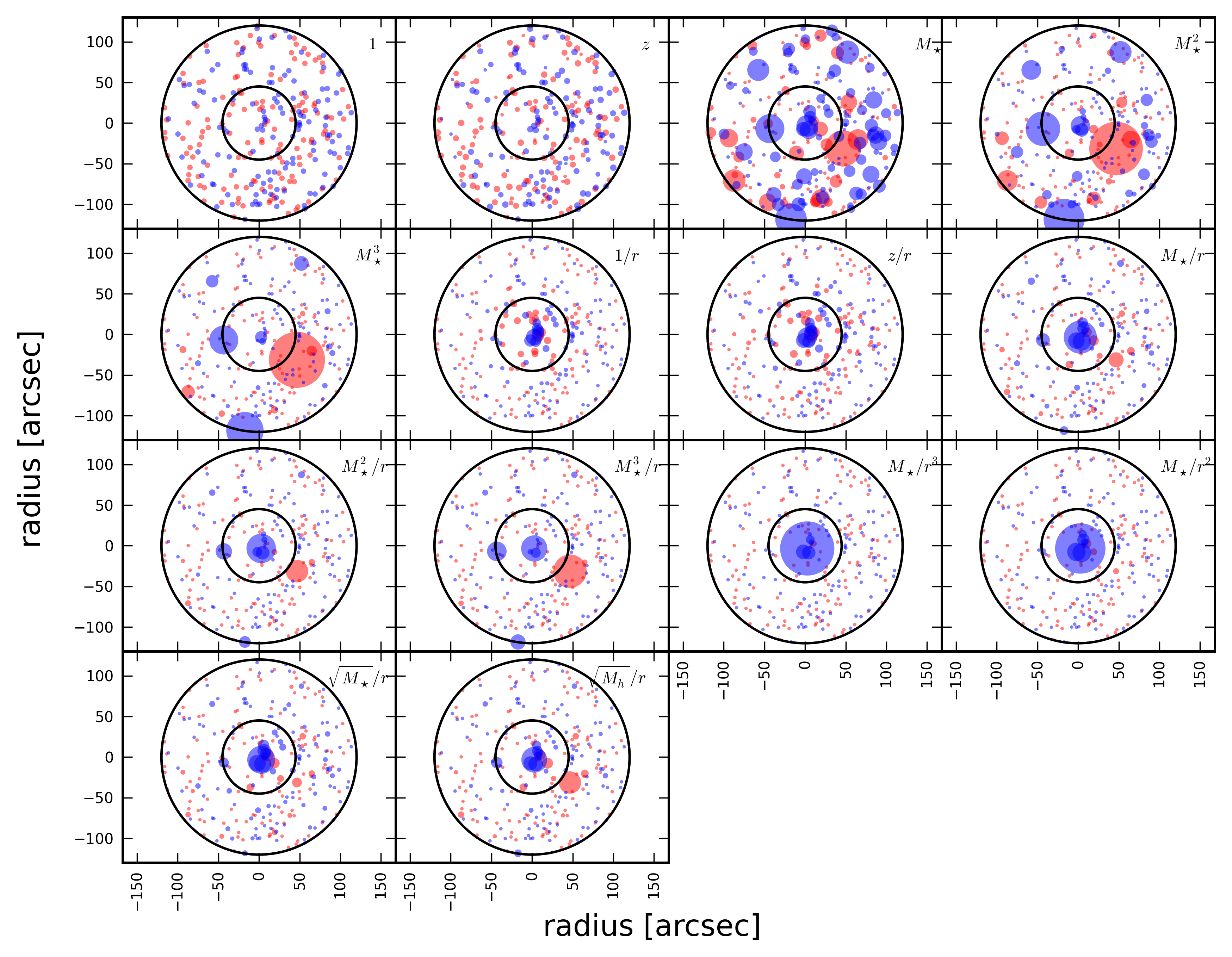
Finally, in Figure 4 we show the relative weight of each galaxy in the HE 04351223 field, where we mark our magnitude and aperture limits. As designed, galaxies very close to the lens have larger weight, particularly for and , as are more massive, and comparatively brighter galaxies.
5.2 Resulting distributions for
In section we present our results, regarding the distribution of overdensities. The results are robust to different sources of systematic and random uncertainties, as we show in detail in Appendix A. The uncertainties discussed in the Appendix include the choice of different aperture radii ( and ) and limiting magnitudes ( and ), using CFHTLenS cells with at least 75% or 50% of their surface free of masks, considering the W1-W4 CFHTLenS individually in order to assess sample variance, and sampling from the inferred distribution of redshift and stellar mass for each galaxy.
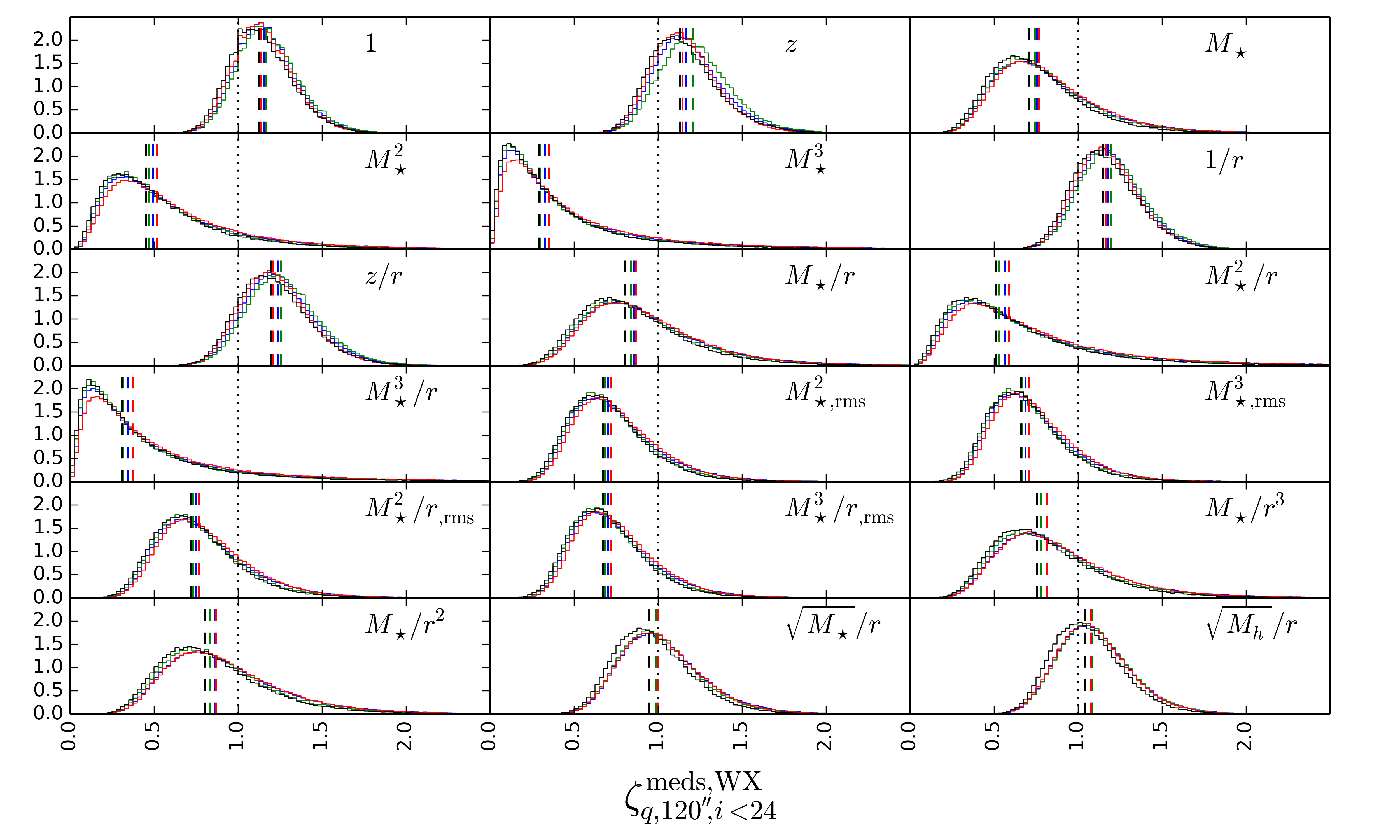
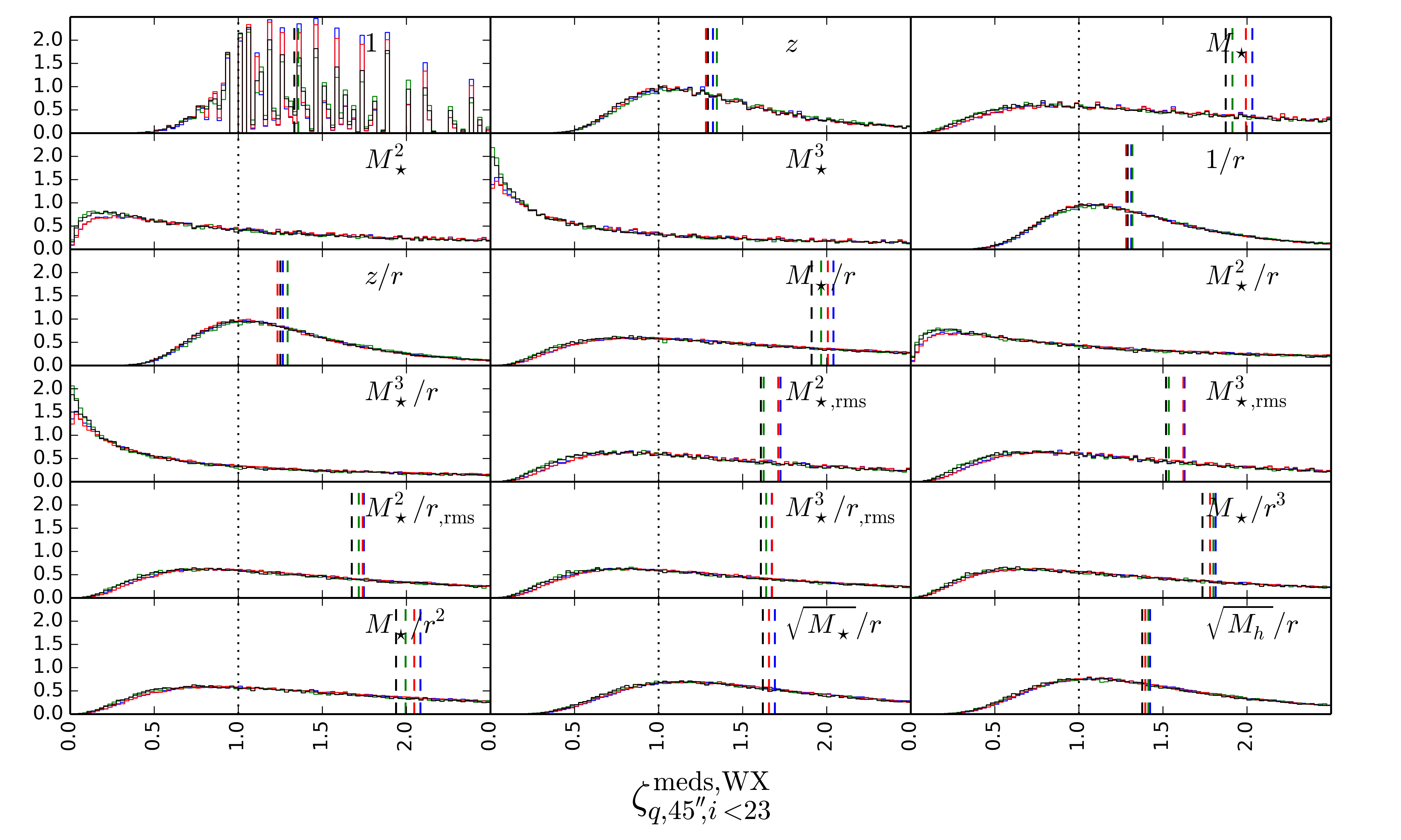
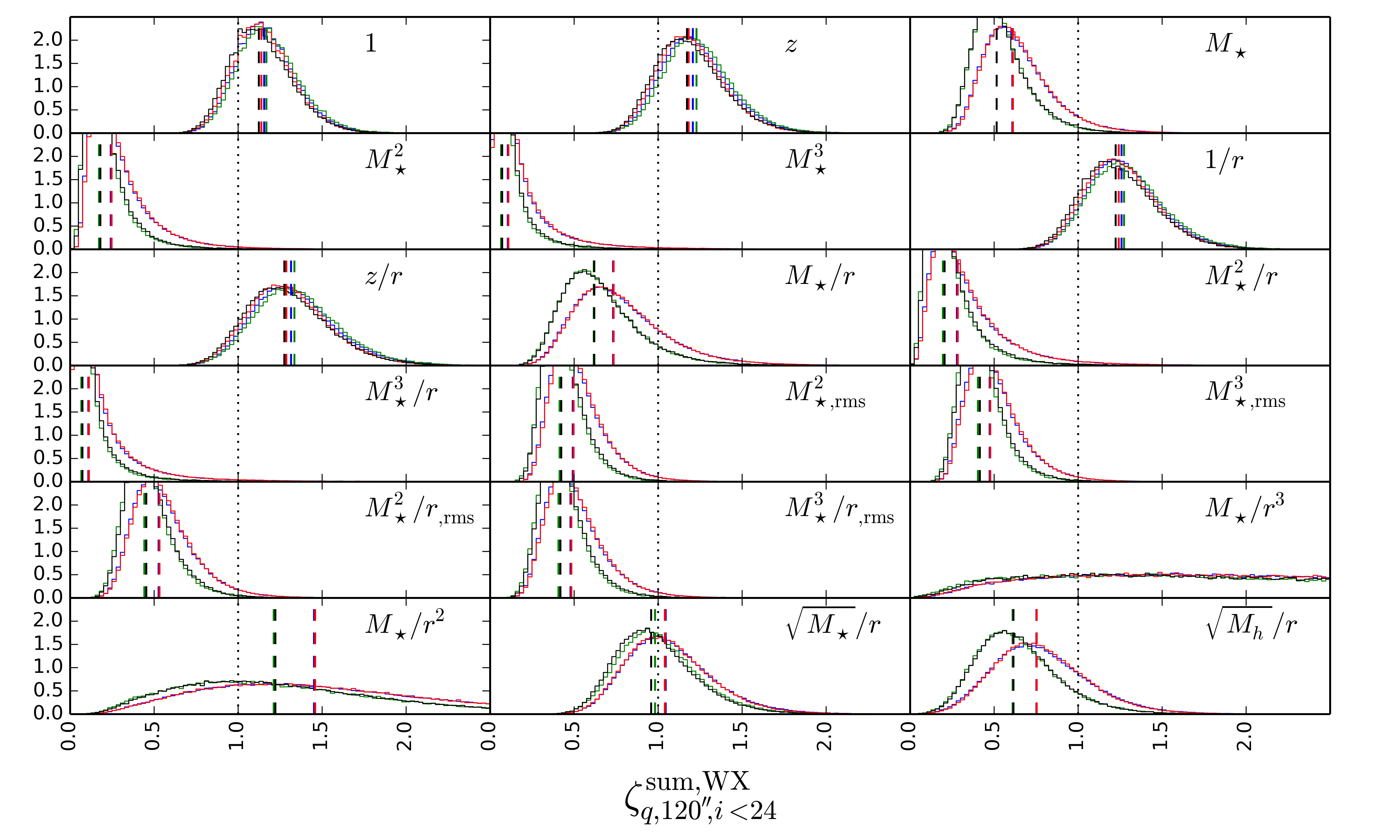
We plot for all weights as well as a selection of aperture radii and limiting magnitudes, in Figures 5, 16 and 17. These are known as ratio distributions, or, more approximately, inverse gaussian distributions. There are two reasons why we take the medians of these distributions as an estimate of the field under/overdensity, , instead of the mean. First, because the median is robust to the long tails displayed by some of the distributions, whereas the use of means would imply that the field is of unphysically large overdensity. Second, so that we can use a numerical approximation which decreases significantly the computation time when estimating weighted count ratios in the MS (see Section B for details). This approach is much faster and more robust than clipped averages.
By comparing the distributions for different magnitude and aperture limits (Figures 5 and 16), it is apparent that the distributions corresponding to brigher limiting magnitude and smaller aperture are wider. This is due to larger Poisson noise when computing weighted counts, since fewer galaxies are included. In Figures 5 and 17 we show the distributions for and , respectively. shows more scatter between W1-W4, and as we will show in Section 6, it is also more noisy. It also shows more clearly that fields W1 and W3 are relatively more similar to each other, and different from W2 and W4, as expected from the fact that these two latter fields have a larger fraction of star contaminants (see Section A). We find that distributions using cells with masked fractions and are very similar, at level. The scatter in for a given weight (hereafter we only consider W1 and W3, given the result above) is also very small, indicating that sample variance in CFHTLenS is not an issue. The distributions are virtually unchanged if we compute stellar masses with or without the IRAC bands, and very similar whether EAZY or BPZ are used to compute redshifts. We find the largest differences when using different SExtractor detection parameters (in particular for the deeper magnitude limit of mag), and when comparing the 10 distributions obtained from sampling from the redshift and stellar mass distributions of each galaxy (see Section A). In Table 5, we give the measured weighted ratios, where we include when computing the medians all the source of scatter discussed above.
| Weight | ||||||||
|---|---|---|---|---|---|---|---|---|
| sum | meds | sum | meds | sum | meds | sum | meds | |
Medians of weighted galaxy counts for HE 04351223, inside various aperture radii and limiting magnitudes. The errors include, in quadrature, scatter from 10 samplings of redshift and stellar mass for each galaxy in HE 04351223, scatter from W1 and W3, BPZ - EAZY, and two different SExtractor detections.
Figure 6 shows a radial plot of the measured overdensity for each weight, for four different aperture radii: , , and . The HE 04351223 field is comparatively more overdense for the brighter limiting magnitude () and, at the brighter limiting magnitude, for the aperture.
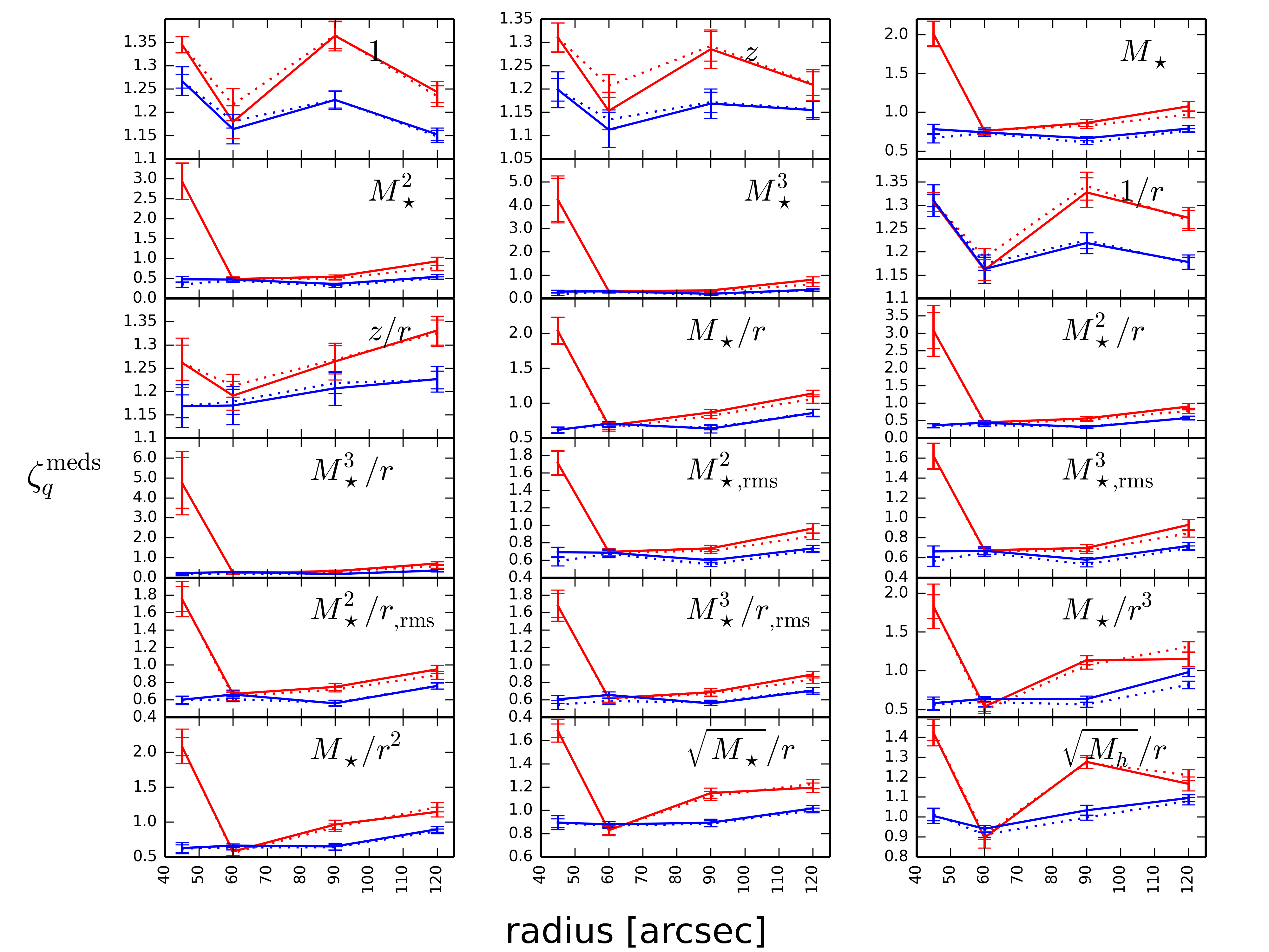
We note that the unweighted count overdensity we measure inside , for , is larger that the underdensity of 0.89 (, assuming simple Poisson noise), measured by Fassnacht, Koopmans, & Wong (2011) inside the same aperture. This is likely due to the deeper magnitude limit they used, their much smaller control field, as well as possibly the use of a less careful masking technique. The present result supercedes the earlier analysis.
5.3 Computing simulated in the MS
Here, we compute weighted count ratios from simulated fields obtained from the Millennium Simulation (MS, Springel et al., 2005), trying to closely reproduce the data quality of the HE 04351223 and the CFHTLenS fields. We do this for two main reasons: First, since we will infer by selecting lines of sight of specific overdensities from the MS, we need to ensure that it is fair to compare the overdensities in the MS to those in the real data. Second, by using the MS we can compare the overdensities we measure with their “true” values, and thus assess the quality of our estimates.
The MS is an -body simulation of cosmic structure formation in a cubic region Mpc of co-moving size, with a halo mass resolution of (corresponding approximately to a galaxy with luminosity ). Catalogues of galaxies populating the matter structures in the simulation were generated based on the semi-analytic galaxy models by De Lucia & Blaizot (2007), Guo et al. (2011) and Bower et al. (2006). Furthermore, 64 simulated fields of deg2 where produced from the MS by ray-tracing (Hilbert et al., 2009). These simulated fields contain, among other information, the observed positions, redshifts, stellar masses, and apparent magnitudes (e.g. in the SDSS and 2MASS filters) of the galaxies in the field, as well as the gravitational lensing convergence and shear as a function of image position and source redshifts.
We use each of the MS fields, in turn, as fields whose overdensities we want to measure (“HE 04351223-like fields”), as well as fields against which we measure those overdensities (“control fields”). For the HE 04351223-like fields we consider only their photometry, whereas for the calibration fields we use their photometry. Based on these, we compute photometric redshifts and stellar masses for all million mag galaxies, using the same techniques we employed for the real data. This is because the stellar masses and redshifts in our real data suffer from observational uncertainties, which are not present in the available synthetic catalogues. For each galaxy, we randomly sample its “observed” magnitude in a given band from a gaussian around its catalogue magnitude, with a standard deviation given by the typical photometric uncertainty of galaxies of similar magnitude in the real data. In Figure 7 we compare the redshifts and stellar masses estimated for the galaxies in the MS with the catalogue values, using photometry based on the De Lucia & Blaizot (2007) semi-analytic models. We find better results compared to the catalogues based on Guo et al. (2011) and Bower et al. (2006), and therefore we use the De Lucia & Blaizot (2007)-based catalogue throughout this work. The photometric redshift bias, scatter and fraction of outliers are comparable to the ones measured for CFHTLenS and HE 04351223 field galaxies. We stress here that the superiority of the De Lucia & Blaizot (2007) semi-analytic models is likely a consequence of these models being more similar to the templates used by BPZ and Le PHARE. However, we are only interested in the empirical result that by using these models we obtain similar uncertainties in the simulations, and in the real data. We thus conclude that we can indeed use the MS galaxy catalogue to estimate overdensities with uncertainties similar to those found in the real data.

We consider the same apertures and limiting magnitudes we used in the real data. In addition, we use the fact that a specific fraction of galaxies in the real HE 04351223 field have spectroscopic redshift, as a function of magnitude and aperture radius. For these galaxies, we use their “true”, catalogue redshifts. We calculate stellar masses with Le PHARE, in the same way we did for the real data, in particular using the same templates. There are, however, several differences to our approach, compared to the real data, which we present in Appendix B.

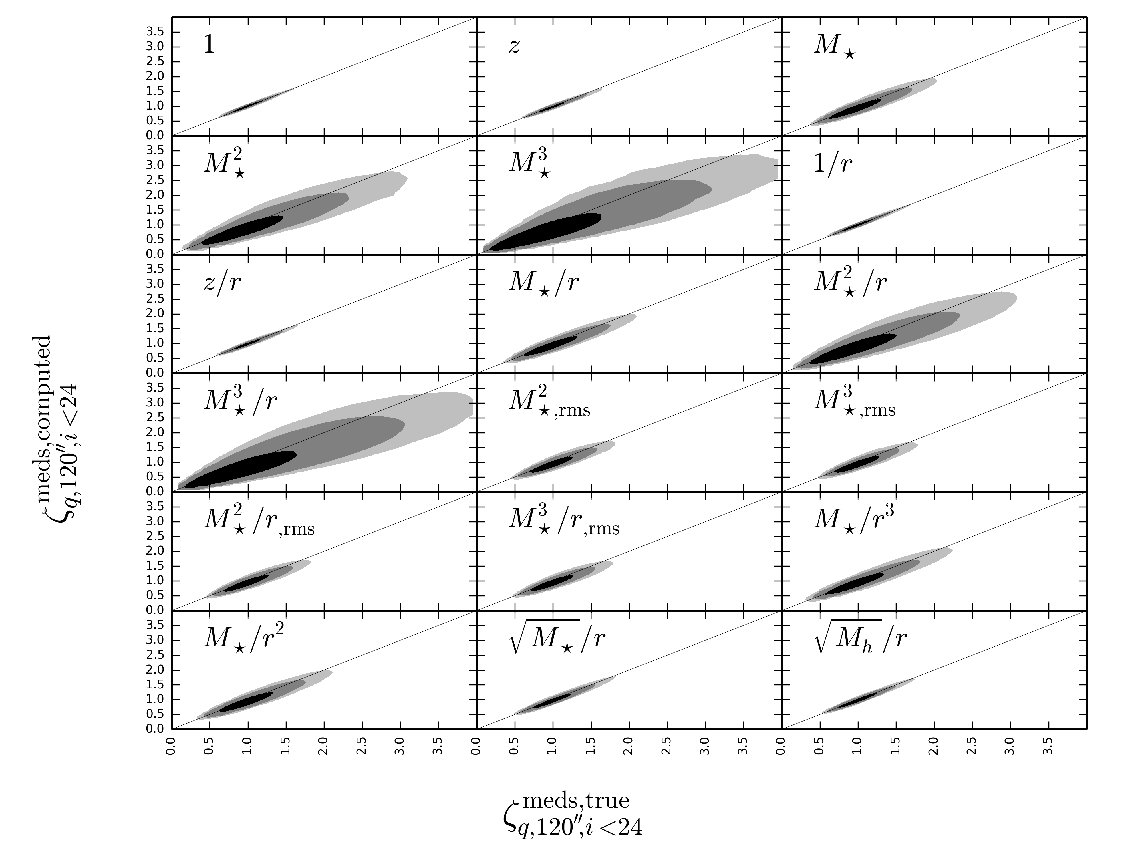
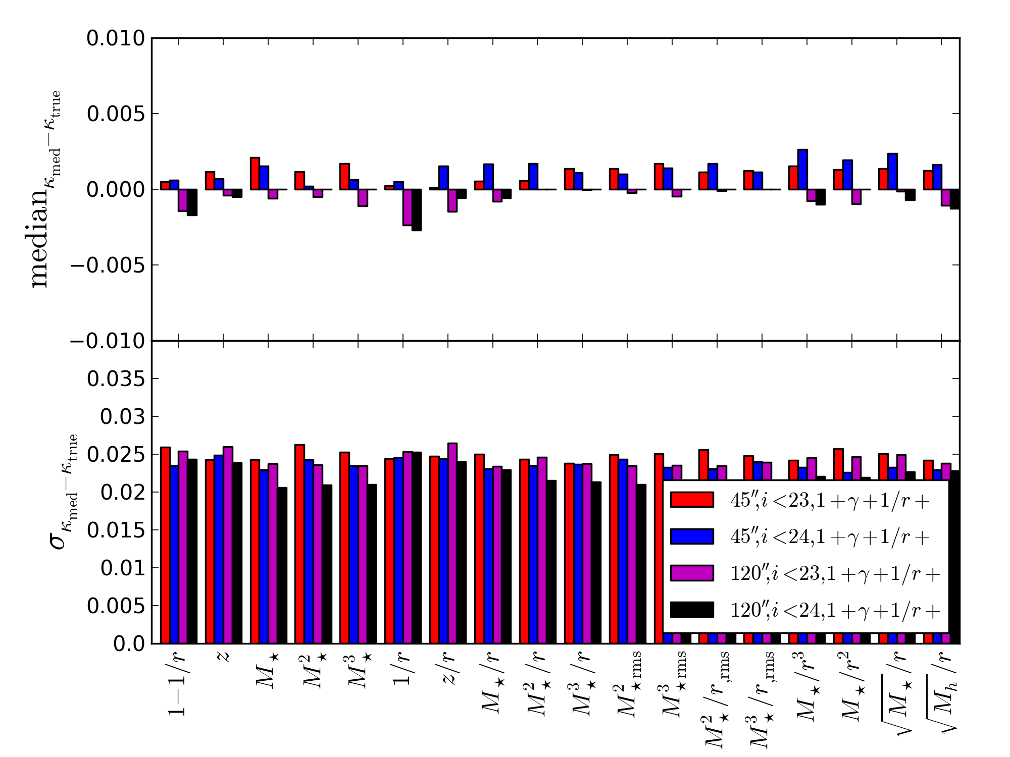
Next, we test how the “measured” overdensities compare to “true” overdensities, obtained by using the “true” values of redshift and stellar mass for each galaxy, readily available in the catalogue for the whole MS. We show the comparisons for and in Figures 8 and 9, respectively. is a much noisier estimate than , and this is particularly obvious for all weights incorporating stellar mass, due to the high dynamic range of this quantity. This justifies our definition of as a better estimate.
We have also checked that a larger aperture radius and fainter magnitude limit produces smaller scatter, which is expected because they include more galaxies, resulting in less Poisson noise; the improvement is much more dependent on radius than on magnitude.
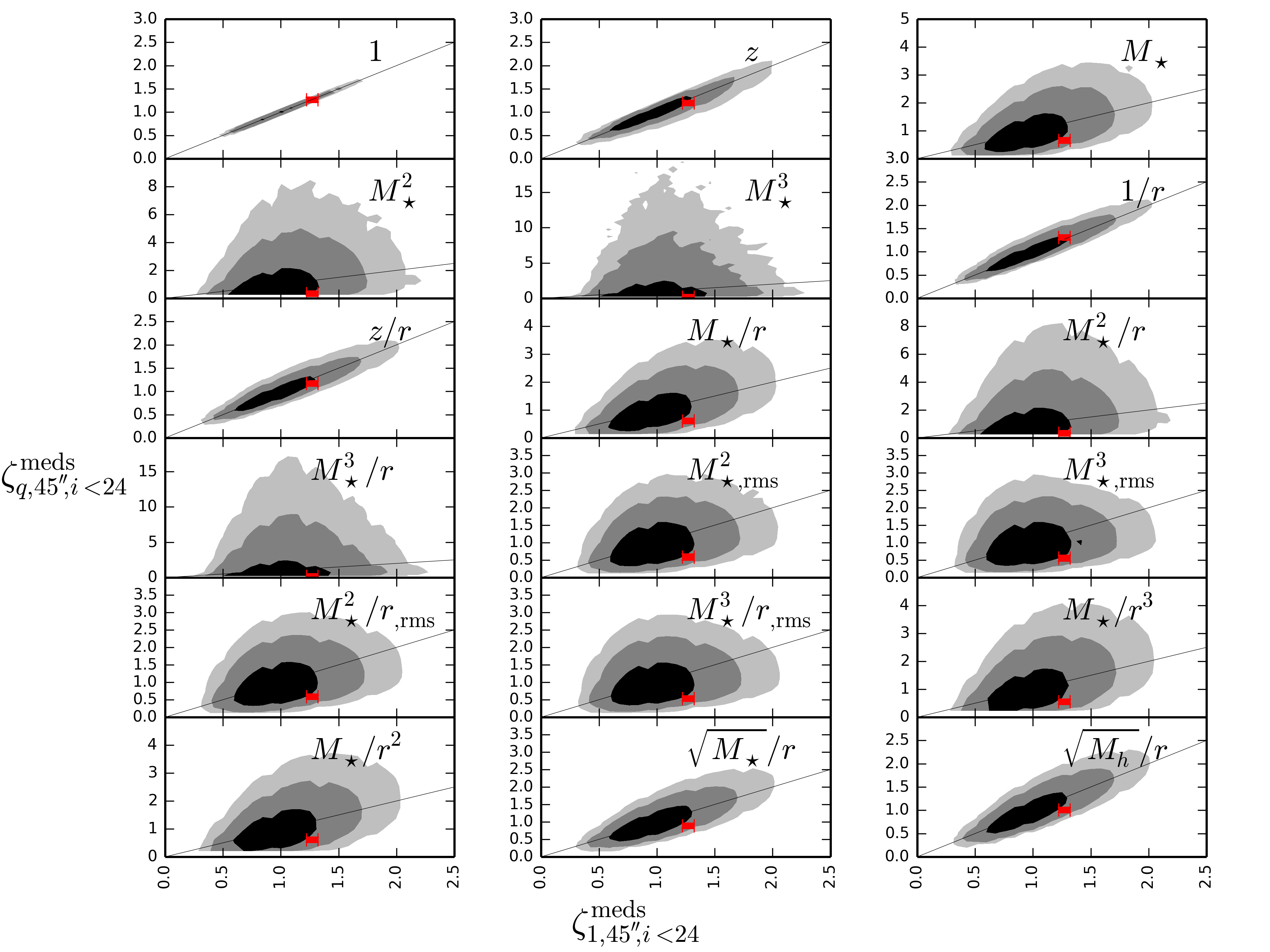
Finally, in Figure 10 we show the relations between the different . We find that the different are correlated, as expected from their definitions, and that the specific values we determined for the HE 04351223 field are realistic, in the sense that the they are expected at -. We have checked that this result is robust to changing the aperture radius and limiting magnitude.
By this point, we have related the points (centers of each cell) in the 64 fields of the MS, where refers to each available cell, to their corresponding . In addition, we have also recorded the corresponding values of the shear , to use as an additional constraint. H0LiCOW Paper IV measured a constant external shear strength (in addition to the shear stemming from explicit mass models of the strong-lens and nearby galaxies) which is close to the median of the shear distribution through the MS. This is helpful for ruling out high values from the distribution (see Figure 8 in Collett et al. (2016). Our use of all available points in the MS (most of which are not strong-lensing lines of sight) is justified by Hilbert et al. (2009) and Suyu et al. (2010), which showed that the distribution of from lines of sight to a strong lens is very similar to, and can be approximated by, the distribution for normal lines of sight (i.e. without a strong lens). We note that the redshift of the source quasar in HE 04351223, , lies between two redshift planes in the MS, at and . We therefore adopted the mean of the two planes for each value of the convergence and shear . 777While there are noticeable differences between individual values, we have determined separately for a single plane, and found that the impact on the distribution is negligible, as the median of inferred P changes by only if we assume the source is at .
6 Determining
In the previous sections, we have explained how we estimate weighted count ratios for the real data, and analogously for the MS, and we have related every point in the MS to the corresponding weighted count ratio around its line of sight. We now present the mathematical formalism and implementation necessary to obtain the distribution of given our knowledge of weighted count ratios around HE 04351223.
6.1 Theory and implementation
We aim to estimate using the MS catalogue of points, in a fully Bayesian framework. By we refer to , where stands for the available data, and we have made our dependence on the data explicit. The data refers to our catalogue of galaxies inside a given aperture and magnitude threshold, for both the HE 04351223 and the CFHTLenS fields. It includes the galaxy number, galaxy positions in their respective apertures, as well as redshifts and stellar masses. In the sections above, we used these data in order to infer , which we denote below as , and is by construction a noisy quantity. We use as a random variable, whose connection to the data and the external convergence can be expressed by a joint distribution . Then, can be expressed as:
| (4) |
Next, we make the assumption that
| (5) |
i.e. the likelihood of the data does not explicitly depend on the external convergence, for fixed . This is justified, since we have defined based solely on the data, without reference to the external convergence. From this,
| (6) |
and thus
| (7) |
That is, given our estimate of from the data, by using a correspondence between and , we obtain the distribution. Here, we consider to be a gaussian with mean and standard deviation given by Table 5, and we make use of the MS by replacing with .
As mentioned in Section 1, G13 showed that the standard deviation of , which we denote as , can decrease when information is added by using multiple conjoined weights. They found the best improvement when using combinations of three weights, including and . We make use of this result, and consider a third weight from those in Section 5.1, in addition to the shear constraint. Thus, our distribution becomes
| (8) |
We determined from the data independently for each , as gaussians much narrower than the distributions whose medians they represent (e.g., Figures 5 and 16). We can thus factorize
| (9) |
We remind the reader that in general (i.e. over the whole extent of their distribution) the are correlated, as we have seen in Section 5.3, and not independent. 888We tested that the approximation in Equation 9 is justified, by measuring the correlation coefficients between , , and to be (at most , in rare cases), for the relevant narrow range of interest.
G13 showed that simply adding up points corresponding to lines of sight with (this generalizes to ), would bias . Here is the median number of galaxies in an aperture of interest around a given line of sight from the MS, and we choose to be twice the width of . The bias comes from the fact that, e.g., for a relatively overdense field, the number of lines of sight available with a galaxy count will be larger than that with a galaxy count (i.e., there are comparatively fewer fields more overdense than a field which is already overdense). A larger number of lines of sight means that their respective distribution will be overrepresented, and the overall will be biased towards those values. The solution adopted by G13 is to divide the interval into bins of individual length 1999In practice, in order to reduce dimensionality, we allow the bins to be as large as 2. G13 (see their Figure 1) showed that this introduces negligible differences. (for this corresponds to incrementing by 1), and weight the distribution in each of the bins by , where is the number of lines of sight in that particular bin. This way, each of the distributions carries equal weight into the combined distribution. In our case, we typically use four conjoined constraints , and therefore have multidimensional bins.
We account for the bias discussed above and compute as a series of nested sums
| (10) |
where and is the number of lines of sight in each multidimensional bin with indices , and is the distribution of corresponding to each of these lines of sight.
For brevity, we refer to implemented by Equation 10 as . We also consider selected distributions with fewer constraints. There are two practical limitation in not using more than four conjoined constraints. First, applying Equation 10 is computationally intensive, and scales quickly with the number of dimensions. Second, the MS contains a limited number of points, and the number of such points included in a bin decreases as additional constraints are added.
6.2 Testing for biases using simulated data
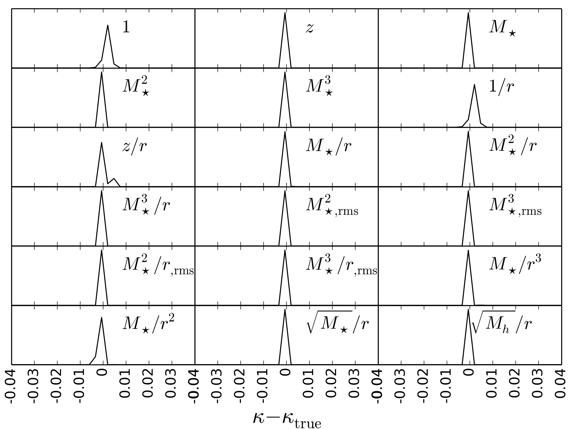
It is possible to use the MS itself to estimate the accuracy of our estimation, and test for biases. First, we randomly select 5000 cells from the MS, which are similar in terms of overdensity to HE 04351223. We then estimate for each of them. However, since this estimation would be computationally expensive, we consider very small uncertainties around the computed overdensities, so that Equation 10 reduces to the computation of a single distribution, in one bin. For each of the 5000 distributions, we record its median, . We then determine the distribution of , where is the true value at the center of each cell. We plot in Figure 11 the median and standard deviation of this distribution, for each weight combination, as well as aperture radius and limiting magnitude. We find that is typically an unbiased estimate of , to better than . For the aperture seems to slightly overestimate , whereas the aperture shows the opposite tendency. These estimates are noisy, with a standard deviation of . This is to be expected: being the median of a distribution of values, cannot vary too much, compared to the individual points. However, the standard deviations of the 5000 individual distributions are also , which means that is typically well-contained inside the individual distributions.
Next, we follow the example of Collett et al. (2013) in assessing the presence of biases in our estimation of the full distribution. In the absence of biases, is centered on zero. For different cells, these offset distributions can be multiplied together, resulting in a narrower distribution . Offsets from zero in the centroid of this distribution would be indicative of biases. We show the results of this approach in Figure 12, where we adopt , and find no indication of offsets for any of the weights we consider. We conclude that, for fields of overdensity similar to HE 04351223, our technique is not affected by biases.
7 Results and Discussion
| q | ||||
|---|---|---|---|---|
The pairs on each column represent (, ). Here
refers to conjoined weights .
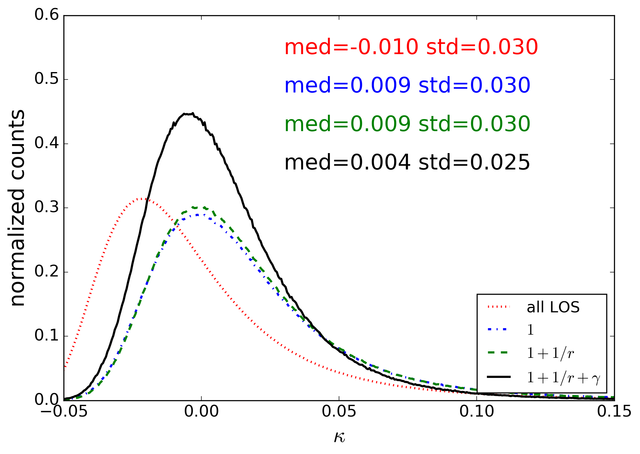
We first present the results on the distribution of external convergence in Figure 13. The HE 04351223 field is slightly overdense in terms of unweighted galaxy counts for aperture radius , mag, resulting in a slightly positive of 0.009. The addition of the radial dependence constraint, , has a very small effect on the distribution. As expected, since the measured shear is similar to the median one through the MS, adding the shear constraint has the effect of narrowing the distribution, and moving it towards lower of 0.004.
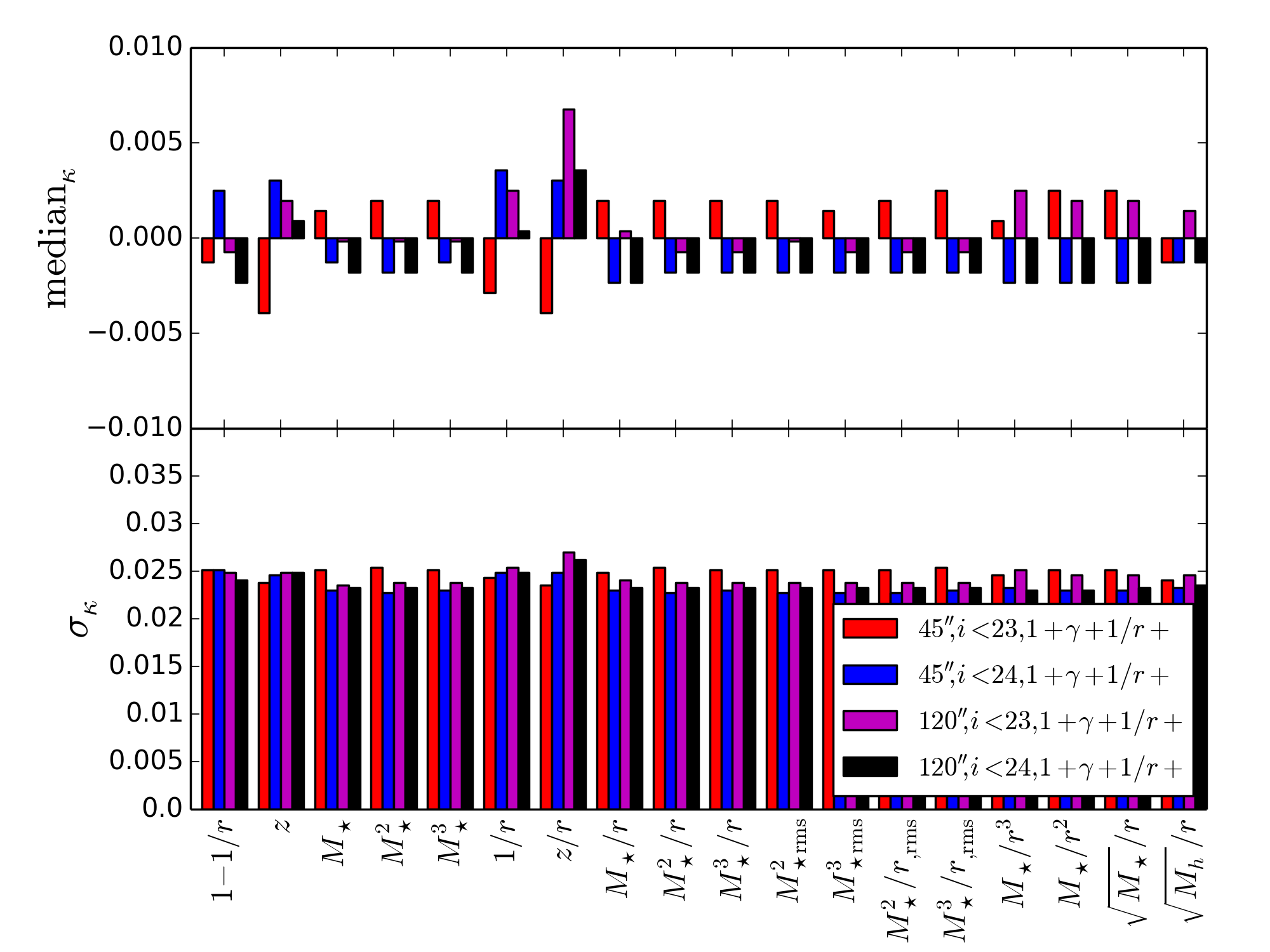
We show the resulting medians and standard deviations of the distributions for all weight combinations, as well as aperture radii and limiting magnitudes, in Figure 14, and summarize the results in Table 6. We find that the addition of weighted count constraints, on top of the constraints from shear, unweighted number counts and distance to the lens, only moves the peak and width of the distributions by . This is expected, since G13 find that the use of weighted count constraints does not yield much improvement for fields of typical overdensities, such as HE 04351223. As a result, we do not expect further improvement if using more than 4 conjoined constraints. The standard deviations of each of the distributions are , which is similar to the values G13 find for fields of comparable overdensities; we note, however, that G13 did not use shear as a constraint. 101010We also checked that changing the shear constraint by towards lower values lowers by .
The shift value at which the distributions are consistent with each other, , even if different apertures and limiting magnitudes are considered, corresponds to impact on , according to Equation 3. Combined with the result from Section 6.2, that our technique is free of biases, this means that our approach is insensitive to the exact choice of aperture and limiting magnitude, among those we explored, at this level. That is, our small, bright limit is already large and deep enough for our analysis. In contrast, as we consider larger and larger apertures, we would expect that we wash away signal, unless we weigh by something steeper than 1/r, because we include larger numbers of galaxies which may be too distant to contribute to . Given large enough apertures, they will tend to an unweighted count ratio of unity regardless of the field. The same argument would hold for deeper magnitudes, except that we implement a cut at the redshift of the source quasar, so going deeper does not imply that we contaminate the signal. The consistency of our results indicates that our large, deep limits are still sensitive to the desired . Finally, the mutual consistency of the distributions for the two limiting magnitudes also ensures that our results are not affected by possible incompleteness111111Though an estimate of completeness is not available for CFHTLenS, for the shallower CFHTLS parent catalogue this is 80% for extended sources of mag, according to http://www.cfht.hawaii.edu/Science/CFHLS/T0007/T0007-docsu12.html.
We note that the small value we measure, well consistent with zero, is also in agreement with the weak lensing upper limit on convergence for this system (Tihhonova et al., in prep.), and the unlikely existence of large structures such as groups, significant enough to boost the convergence (H0LiCOW Paper II).
8 Conclusions and future work
In this work, we aimed to estimate a robust probability distribution function of the external convergence for HE 04351223, in order to enable the use of this lens system as an accurate probe of . We used spectroscopy and multiband images of the HE 04351223 field, and we used the wide component of CFHTLenS as a control field. Building on the work by G13, we refined the method in order to cope with the large fraction of masks in our control field, and we also used more robust medians rather than sums in order to compare weighted counts. We thoroughly explored sources of error in our data sets, such as mask coverage, galaxy-star classification, detection efficiency etc.; we propagated these into the computation of weighted count ratios, finding that the HE 04351223 field is more overdense, in terms of number counts, than previously estimated. We used the whole extent of the MS to simulate photometric data of the same quality, and connect the MS lensing convergence catalogue to synthetic weighted count ratios estimated in a similar way. We than estimated the probability distribution function of the external convergence for fields similar in overdensity to HE 04351223, in a Bayesian, unbiased way.
We considered multiple aperture radii and limiting magnitudes, and tested them using the MS, finding that a aperture and a limiting magnitude of provide enough spatial coverage and depth to estimate the distribution of external convergence via the weighted counts technique. We find that our different estimates are consistent with each other at a level of , corresponding to impact on . Our estimate which is least affected by photometric redshifts and stellar mass uncertainties, , has a median of 0.004, and a standard deviation of 0.025. This uncertainty contributes rms error to the value of . We intend to employ the techniques developed in this paper for the analysis of the other H0LiCOW lens systems. In particular, HE 04351223 is a rather typical line of sight, and we expect that lenses residing in comparatively overdense fields will benefit more from the use of additional constraints including photometric redshifts and stellar masses.
Throughout this work, we have made extensive use of the MS. The weighted count ratios technique is designed to minimize our reliance on a particular simulation, but it will be useful to repeat this analysis by using simulations for different cosmologies and galaxy models to test any remaining dependencies. However, we expect such dependencies to be small, given that the external convergence we measure is close to zero. Assuming a simple linear deterministic galaxy bias model, the convergence inferred from a given relative galaxy number overdensity scales roughly with the mean matter density parameter and the matter density fluctuation amplitude (see Section C). Therefore, for example, . For , this corresponds to impact. We leave further checks for future work, as other simulations with convergence maps become available.
Recently, McCully et al. (2016) presented a technique of reconstructing the external convergence without relying on a particular simulation, through a direct modelling of the field. This has the potential of further reducing the uncertainty on the external convergence. This work has produced the galaxy catalogues necessary for a future implementation of that technique. While we have accounted in this work for the presence of voids, groups and clusters statistically, through the use of the MS, our catalogue products are also used in separate works (H0LiCOW Paper II and Tihhonova et al., in prep.) to directly identify such structures.
Acknowledgments
The authors would like to thank Jean Coupon, Thomas Erben, Hendrik Hildebrandt, Yagi Masafumi, Samuel Schmidt, and Ichi Tanaka for helpful discussions. Also, Adam Tomczak for providing the PSF matching code. C.E.R and C.D.F. were funded through the NSF grant AST-1312329, “Collaborative Research: Accurate cosmology with strong gravitational lens time delays”, and the HST grant GO-12889. DS acknowledges funding support from a Back to Belgium grant from the Belgian Federal Science Policy (BELSPO). S.H. acknowledges support by the DFG cluster of excellence ‘Origin and Structure of the Universe’ (www.universe-cluster.de). K.C.W. is supported by an EACOA Fellowship awarded by the East Asia Core Observatories Association, which consists of the Academia Sinica Institute of Astronomy and Astrophysics, the National Astronomical Observatory of Japan, the National Astronomical Observatories of the Chinese Academy of Sciences, and the Korea Astronomy and Space Science Institute. S.H.S. acknowledges support from the Max Planck Society through the Max Planck Research Group. This work is supported in part by the Ministry of Science and Technology in Taiwan via grant MOST-103-2112-M-001-003-MY3. T.T. thanks the Packard Foundation for generous support through a Packard Research Fellowship, the NSF for funding through NSF grant AST-1450141, “Collaborative Research: Accurate cosmology with strong gravitational lens time delays”. LVEK is supported in part through an NWO-VICI career grant (project number 639.043.308).
Data analysis was in part carried out on common use data analysis computer system at the Astronomy Data Center, ADC, of the National Astronomical Observatory of Japan, as well as the SLAC National Accelerator Laboratory.
This work is based in part on observations obtained with MegaPrime/MegaCam, a joint project of CFHT and CEA/IRFU, at the CFHT which is operated by the National Research Council (NRC) of Canada, the Institut National des Sciences de l’Univers of the Centre National de la Recherche Scientifique (CNRS) of France, and the University of Hawaii. It is also based in part on observations made with the Spitzer Space Telescope, which is operated by the Jet Propulsion Laboratory, California Institute of Technology under a contract with NASA, and on observations obtained at the Gemini Observatory, which is operated by the Association of Universities for Research in Astronomy, Inc., under a cooperative agreement with the NSF on behalf of the Gemini partnership: the National Science Foundation (United States), the National Research Council (Canada), CONICYT (Chile), the Australian Research Council (Australia), Ministério da Ciência, Tecnologia e Inovação (Brazil) and Ministerio de Ciencia, Tecnología e Innovación Productiva (Argentina).
The authors recognize and acknowledge the very significant cultural role and reverence that the summit of Mauna Kea has always had within the indigenous Hawaiian community. We are most fortunate to have the opportunity to conduct observations from this superb mountain.
TOPCAT (Taylor, 2005) was used for catalogue matching. The codes developed during the course of this work are publicly available at https://github.com/eduardrusu/zMstarPDF.
References
- Bar-Kana (1996) Bar-Kana R., 1996, ApJ, 468, 17
- Behroozi, Conroy, & Wechsler (2010) Behroozi P. S., Conroy C., Wechsler R. H., 2010, ApJ, 717, 379
- Benítez (2000) Benítez N., 2000, ApJ, 536, 571
- Bertin & Arnouts (1996) Bertin E., Arnouts S., 1996, A&AS, 117, 393
- Bertin et al. (2002) Bertin E., Mellier Y., Radovich M., Missonnier G., Didelon P., Morin B., 2002, ASPC, 281, 228
- Bertin (2006) Bertin E., 2006, ASPC, 351, 112
- Boulade et al. (2003) Boulade O., et al., 2003, SPIE, 4841, 72
- Bower et al. (2006) Bower R. G., Benson A. J., Malbon R., Helly J. C., Frenk C. S., Baugh C. M., Cole S., Lacey C. G., 2006, MNRAS, 370, 645
- Brammer, van Dokkum, & Coppi (2008) Brammer G. B., van Dokkum P. G., Coppi P., 2008, ApJ, 686, 1503
- Bruzual & Charlot (2003) Bruzual G., Charlot S., 2003, MNRAS, 344, 1000
- Buton et al. (2012) Buton C., et al., 2012, yCat, 354, 90008
- Chabrier (2003) Chabrier G., 2003, PASP, 115, 763
- Collett et al. (2013) Collett T. E., et al., 2013, MNRAS, 432, 679
- Collett et al. (2016) Collett T. E., Cunnington, S., 2016, arXiv, arXiv:1605.08341
- Erben et al. (2013) Erben T., et al., 2013, MNRAS, 433, 2545
- Falco, Gorenstein, & Shapiro (1985) Falco E. E., Gorenstein M. V., Shapiro I. I., 1985, ApJ, 289, L1
- Fassnacht et al. (2006) Fassnacht C. D., Gal R. R., Lubin L. M., McKean J. P., Squires G. K., Readhead A. C. S., 2006, ApJ, 642, 30
- Fassnacht, Koopmans, & Wong (2011) Fassnacht C. D., Koopmans L. V. E., Wong K. C., 2011, MNRAS, 410, 2167
- Fazio et al. (2004) Fazio G. G., et al., 2004, ApJS, 154, 10
- Le Fèvre et al. (2005) Le Fèvre O., et al., 2005, A&A, 439, 845
- Garilli et al. (2008) Garilli B., et al., 2008, A&A, 486, 683
- Guo et al. (2011) Guo Q., et al., 2011, MNRAS, 413, 101
- Greene et al. (2013) Greene Z. S., et al., 2013, ApJ, 768, 39
- Gwyn (2012) Gwyn S. D. J., 2012, AJ, 143, 38
- Heymans et al. (2012) Heymans C., et al., 2012, MNRAS, 427, 146
- Hilbert et al. (2009) Hilbert S., Hartlap J., White S. D. M., Schneider P., 2009, A&A, 499, 31
- Hildebrandt et al. (2010) Hildebrandt H., et al., 2010, A&A, 523, A31
- Hildebrandt et al. (2012) Hildebrandt H., et al., 2012, MNRAS, 421, 2355
- Hodapp et al. (2003) Hodapp K. W., et al., 2003, PASP, 115, 1388
- Ichikawa et al. (2006) Ichikawa T., et al., 2006, SPIE, 6269, 626916
- Ilbert et al. (2006) Ilbert O., et al., 2006, A&A, 457, 841
- Ilbert et al. (2010) Ilbert O., et al., 2010, ApJ, 709, 644
- Keeton & Zabludoff (2004) Keeton C. R., Zabludoff A. I., 2004, ApJ, 612, 660
- Kobayashi et al. (2000) Kobayashi N., et al., 2000, SPIE, 4008, 1056
- De Lucia & Blaizot (2007) De Lucia G., Blaizot J., 2007, MNRAS, 375, 2
- Lucy (1974) Lucy L. B., 1974, AJ, 79, 745
- McCully et al. (2016) McCully C., Keeton C. R., Wong K. C., Zabludoff A. I., 2016, arXiv, arXiv:1601.05417
- Merlin et al. (2015) Merlin E., et al., 2015, A&A, 582, A15
- Momcheva et al. (2006) Momcheva I., Williams K., Keeton C., Zabludoff A., 2006, ApJ, 641, 169
- Momcheva et al. (2015) Momcheva I. G., Williams K. A., Cool R. J., Keeton C. R., Zabludoff A. I., 2015, ApJS, 219, 29
- Morgan et al. (2005) Morgan N. D., Kochanek C. S., Pevunova O., Schechter P. L., 2005, AJ, 129, 2531
- Refsdal (1964) Refsdal S., 1964, MNRAS, 128, 307
- Richardson (1972) Richardson W. H., 1972, JOSA, 62, 55
- Schlafly & Finkbeiner (2011) Schlafly E. F., Finkbeiner D. P., 2011, ApJ, 737, 103
- Schneider & Sluse (2013) Schneider P., Sluse D., 2013, A&A, 559, A37
- Scoville et al. (2007) Scoville N., et al., 2007, ApJS, 172, 1
- Sluse et al. (2012) Sluse D., Hutsemékers D., Courbin F., Meylan G., Wambsganss J., 2012, A&A, 544, A62
- Springel et al. (2005) Springel V., et al., 2005, Natur, 435, 629
- Suyu et al. (2010) Suyu S. H., Marshall P. J., Auger M. W., Hilbert S., Blandford R. D., Koopmans L. V. E., Fassnacht C. D., Treu T., 2010, ApJ, 711, 201
- Suyu et al. (2013) Suyu S. H., et al., 2013, ApJ, 766, 70
- Suzuki et al. (2008) Suzuki R., et al., 2008, PASJ, 60, 1347
- Taylor (2005) Taylor M. B., 2005, ASPC, 347, 29
- Treu & Marshall (2016) Treu T., Marshall P. J., 2016, A&ARv, in press, arxiv1605.05333
- Velander et al. (2014) Velander M., et al., 2014, MNRAS, 437, 2111
- Wisotzki et al. (2000) Wisotzki L., Christlieb N., Bade N., Beckmann V., Köhler T., Vanelle C., Reimers D., 2000, A&A, 358, 77
- Wisotzki et al. (2002) Wisotzki L., Schechter P. L., Bradt H. V., Heinmüller J., Reimers D., 2002, A&A, 395, 17
- Wong et al. (2011) Wong K. C., Keeton C. R., Williams K. A., Momcheva I. G., Zabludoff A. I., 2011, ApJ, 726, 84
- Yagi et al. (2013a) Yagi M., Gu L., Fujita Y., Nakazawa K., Akahori T., Hattori T., Yoshida M., Makishima K., 2013, ApJ, 778, 91
- Yagi et al. (2013b) Yagi M. S., Nao, Yamanoi H., Furusawa H., Nakata F., Komiyama Y., 2013, PASJ, 65, 22
Appendix A Exploring systematics and sources of noise in the estimation of weighted count ratios
When measuring the weighted count ratios as described in Section 5.1, we account for several factors and estimate how much they contribute to the total uncertainty:

-
Sample variance. To test the extent to which we are affected by sample variance, as well as by different fractions of stars in the CFHTLenS fields, we do not combine the W1-W4 fields, but measure overdensities for each of them separately. W4 is known to contain a larger fraction of stars (Hildebrandt et al., 2012), and this may impact our results, given our galaxy-star classification, which assumes that all faint objects are galaxies (Section 3). We also expect this to be the case for W2, given its low galactic latitude.121212We used the plots available at http://www.iac.es/proyecto/frida/skyCoverage.html to estimate the relative number of stars, given the galactic coordinates of each field.
-
Fraction of masks. Using CFHTLenS cells with a substantial fraction of their areas covered by masks may introduce large Poisson noise. To estimate this effect, we exclude all cells that have more than 25% and 50%, respectively, of their areas masked. This results in eliminating of the cells ( apertures), and of the cells ( apertures), respectively.
-
Limiting magnitude and aperture radius. To quantify the dependence of our results on the aperture radius and limiting magnitude, we also consider limits of -radius (used by G13) and mag (S/N ), in addition to and .
-
Detection efficiency. In order to avoid biases when estimating weighted counts relative to CFHTLenS, and in view of the similarity between our -band data for HE 04351223 and the CFHTLenS -band, we used the same detection parameters employed for the latter. However, galaxy counts at the limiting magnitude are sensitive to the detection parameters, and we found that by changing the DETECT_THRESHOLD parameter in SExtractor from 1.5 to 2.5, we obtain more robust detections. We therefore consider the scatter between the two detection runs, where for each one we compute weighted ratios for all weights.
-
Detections at the limiting magnitude. Due to uncertainties in the photometry at the limiting magnitude, some galaxies above the magnitude cut are in fact wrongly included in the cut, and vice-versa. This may bias the results. Therefore for all galaxies in the HE 04351223 field we consider a gaussian around their SExtractor-measured -band magnitude, with a standard deviation equal to the size of the photometric error bar, and randomly sample from this to test if the galaxy survives the color cut. We do this for each cell in a CHFTLenS WX field, as we compute . It is unnecessary to do the same for the galaxies inside CFHTLenS, due to the large number of cells.
-
Cell number dependence on the aperture radius. When considering a larger aperture radius around the lens system, and therefore a larger cell size, there are comparatively fewer contiguous non-overlapping cells spanning CFHTLenS. As a result, the distribution will look noisy. To avoid this, we allow cells to partially overlap, with larger overlapping fraction for larger apertures. In practice, we use 2 equally spaced overlaps along each dimension of the -length cells (i.e. along each dimension in the grid, we consider cells centered at length/2, length/2, length/2 etc.), and 5 overlaps for the -length cells, respectively.
-
Different photometric redshift codes, and the importance of the IRAC bands. We include the scatter in the overdensities measured when using BPZ and EAZY separately, to compute photometric redshifts. This potentially affects more than just the weights explicitly incorporating redshift, since we do a cut at the source redshift, and the redshift values also affect the goodness-of-fit used to separate stars from galaxies. We also compute weights for stellar masses calculated with the inclusion of the IRAC channels, as well as without.
-
Accounting for the and of an individual galaxy. Instead of just using the best-fit photometric redshift and median stellar mass for each galaxy in the HE 04351223 field, we sample 10 times from the galaxy’s redshift probability distribution, and compute the associated stellar mass (for which we also sample from the distribution returned by Le PHARE). We then compute for each of these. Again, it is not necessary to do this for the galaxies inside CFHTLenS, due to the large number of cells, which are only used once.
Appendix B Details on inferring weighted count ratios from the MS
Even though we have made every effort to analyze the simulated data in the same manner as the real data, this was not always possible, due to inherent differences and computational reasons. Here we present details of our weighted count ratios estimation from the MS, and the way the approach differs from the real data.
-
The MS catalogues represent a pure and complete sample of galaxies, whereas this is not the case in the real data. As a result, we randomly inject stars and remove galaxies, mirroring the contamination and incompleteness found in the real data. For this, we use the contamination and incompleteness fractions estimated in Figure 9 of Hildebrandt et al. (2012) for the CFHTLenS W1 field, as a function of magnitude. We considered 500 real stars for each 0.5 mag bin from CFHTLenS, and computed for these “redshifts” with BPZ, as well as “stellar masses” with Le PHARE. We then selected from these based on the the contamination fraction, and inserted them at random positions into each aperture of the simulation.
-
It is important to use all the complete spatial extent of the MS (i.e. all MS fields), as our use of multiple conjoined weights when selecting lines of sight of similar overdensities (which we describe in Section 6) implies that we are limited by the number of available points found in the simulation. Each of the 64 MS fields has a corresponding grid of convergence values (we refer to these as points), with spacing. In Section A we described how we use overlapping cells across the CFHTLenS fields. Here we use even higher fractions of overlaps, as we center one cell on each of the points. The only exceptions are at the edges of the fields, where the apertures would fall outside the field.
-
Given the points in the simulation, it is computationally expensive to estimate the weighted count ratios of each of the or aperture cells relative to every other cell, and take the median. In addition, the MS fields do not contain masks, in contrast to the HE 04351223 and CFHTLenS fields. However, as we have seen in Section 5.2, where we compared results after eliminating fields with different fractions of masks, the effect is negligible. The only masks we employ are the radius inner masks around the center of each cell (to account for the fact that in the real data we masked the HE 04351223 system itself, and its most nearby perturber), and the outer or radius representing the circular apertures. As a result, we can make an approximation in computing weighted count ratios. We compute the overdensity for each cell simply as , where . We have checked that this redefinition is numerically indistinguishable from the one in Section 5.1, given the range spanned by . We note, however, that the same approximation would not hold if we used the mean instead of the median.
-
Due to the field of view being slightly smaller than the aperture, of the galaxies around the edge of the HE 04351223 field do not have coverage in these bands. We neglect this in the simulations.
-
The MS catalogues do not contain synthetic magnitudes in the IRAC bands. However, as discussed in Section 5.2, the effect that the exclusion of these bands has for the computation of weighting count ratios incorporating stellar masses is negligible.
-
Since we have a large number of cells, it is unnecessary to repeatedly sample from the magnitudes of the galaxies at the faint limit, like we did for the HE 04351223 field. We also do not sample from the and of each galaxy in the HE 04351223-like fields. Finally, we limit ourselves to the use of BPZ for estimating photometric redshifts.
Appendix C Cosmology dependence of the external convergence estimates
Using a simple galaxy bias model, we can obtain a rough estimate of the cosmology dependence of the external convergence inferred from weighted galaxy counts. To first order in matter density fluctuations, the convergence for sources with angular image position and redshift can be expressed by a weighted projection of the matter density contrast along the line of sight:
| (11) |
Here, denotes the speed of light, , , , , and , where denotes the comoving line-of-sight distance for sources at redshift , and the comoving angular diameter distance for comoving line-of-sight distance . Furthermore, denotes the matter density contrast at comoving transverse position , comoving line-of-sight distance , and cosmic epoch expressed by the redshift . Moreover, denotes the Hubble distance, and denotes the Hubble parameter at redshift .
In a simple linear deterministic galaxy model, the galaxy density contrast is related to the matter density contrast by the relation:
| (12) |
with the galaxy bias parameter as proportionality factor (assumed independent of redshift for simplicity). Assume that the large-scale galaxy correlations and/or power spectra have been observed and their amplitude has been quantified, e.g. by a galaxy fluctuation amplitude parameter defined as the standard deviation of the galaxy density contrast averaged over spheres of . The analogous quantity for the matter density contrast is the cosmic matter fluctuation amplitude . For a given cosmological model and observed galaxy clustering amplitude, the bias parameter can thus be expressed as . Hence,
| (13) |
For all considered cosmologies, , , and are proportional to , and weakly varying with the cosmic mean density parameters , , etc. and equation-of-state parameters , , or . Furthermore, and weakly varying with , , , etc. Thus, to lowest order in cosmological parameters, the convergence inferred from an observed galaxy density contrast (or similar relative galaxy density quantities such as the weighted counts considered in this paper) can be expressed by:
| (14) |
where denotes the inferred convergence assuming cosmological parameters and instead of parameters and , resp. Therefore, for an arbitrary function which depends on the external convergence , this implies:
| (15) |
where denotes the external convergence inferred assuming and .